NWP-Based Adjustment of IMERG Precipitation for Flood-Inducing Complex Terrain Storms: Evaluation over CONUS

1
Department of Civil and Environmental Engineering, University of Connecticut, Storrs, CT 06269, USA
2
National Center for Atmospheric Research, Boulder, CO 80301, USA
*
Author to whom correspondence should be addressed.
Remote Sens. 2018, 10(4), 642; https://doi.org/10.3390/rs10040642
Submission received: 20 February 2018
/
Revised: 12 April 2018
/
Accepted: 15 April 2018
/
Published: 21 April 2018
(This article belongs to the Special Issue Remote Sensing of Precipitation)
Abstract
:This paper evaluates the use of precipitation forecasts from a numerical weather prediction (NWP) model for near-real-time satellite precipitation adjustment based on 81 flood-inducing heavy precipitation events in seven mountainous regions over the conterminous United States. The study is facilitated by the National Center for Atmospheric Research (NCAR) real-time ensemble forecasts (called model), the Integrated Multi-satellitE Retrievals for GPM (IMERG) near-real-time precipitation product (called raw IMERG) and the Stage IV multi-radar/multi-sensor precipitation product (called Stage IV) used as a reference. We evaluated four precipitation datasets (the model forecasts, raw IMERG, gauge-adjusted IMERG and model-adjusted IMERG) through comparisons against Stage IV at six-hourly and event length scales. The raw IMERG product consistently underestimated heavy precipitation in all study regions, while the domain average rainfall magnitudes exhibited by the model were fairly accurate. The model exhibited error in the locations of intense precipitation over inland regions, however, while the IMERG product generally showed correct spatial precipitation patterns. Overall, the model-adjusted IMERG product performed best over inland regions by taking advantage of the more accurate rainfall magnitude from NWP and the spatial distribution from IMERG. In coastal regions, although model-based adjustment effectively improved the performance of the raw IMERG product, the model forecast performed even better. The IMERG product could benefit from gauge-based adjustment, as well, but the improvement from model-based adjustment was consistently more significant.
1. Introduction
Accurate measurement of precipitation is a prerequisite for understanding related hydrologic processes. The fact that precipitation is highly discontinuous in space and time presents challenges for obtaining accurate spatio-temporal quantification of precipitation, especially over topographically-complex regions, due to the variability and uncertainty introduced by orographic effects [1,2]. Generally, observed gridded precipitation datasets can be generated by three approaches: gauge data interpolation, surface radar network and satellite-based observation.
The accuracy of gauge interpolation depends largely on gauge density and measurement quality. Gauge locations are not homogeneously distributed; there are more gauges at low elevations and in densely-populated areas relative to mountainous terrain because of the higher costs of gauge installation and maintenance over complex topography. Moreover, since gauge networks around the world are operated by different countries, the observations are less accessible due to different data-sharing policies. Hence, gauge-based gridded precipitation datasets usually have coarse temporal and spatial resolutions; most global products have monthly or daily time scales and 0.25° to 2.5° spatial resolutions [3,4,5,6].
However, for meso-scale studies of such as extreme rainfall events and related floods, precipitation products with higher spatial and temporal resolution are required. Although surface radar networks provide fine resolution products, the data quality is limited in complex terrain due to severe beam blocking and strong ground clutter [7,8,9]. In addition, considering the expensive operating and maintenance costs, spatial coverages of radar networks are very limited especially in mountainous or less populated regions.
Besides surface observations, techniques of satellite-based measurements have developed rapidly over the past 30+ years [10]. As a result, a variety of satellite-based precipitation products is now available with quasi-global coverage, including the Tropical Rainfall Measuring Mission (TRMM) near-Real-Time Multi-satellite Precipitation product (3B42RT) [11], the National Oceanic and Atmospheric Administration (NOAA) Climate Prediction Center (CPC) morphing technique (CMORPH) [12], the Precipitation Estimation from Remotely Sensed Information Using Artificial Neural Networks (PERSIANN) [13], the Global Satellite Mapping of Precipitation Microwave-IR Combined Product (GSMaP) produced by the Earth Observation Research Center (EORC) of the Japan Aerospace Exploration Agency (JAXA) [14,15] and products of Global Precipitation Measurement (GPM) Integrated Multi-satellitE Retrievals for GPM (IMERG) [16]. Many studies indicate that these satellite products tend to underestimate heavy precipitation over mountainous regions [17,18,19,20,21,22].
Apart from single source datasets, products with combined data sources are available, as well. Typically, gauge observations are incorporated into raw radar or satellite products to improve accuracy [23,24,25]. In fact, most satellite products mentioned above have their gauge-adjusted counterparts [11,16,26,27,28]. In general, gauge-adjusted satellite products are released weeks to months after the observation time because of the delay of high quality gauge datasets, and the accuracy largely depends on the spatio-temporal representativeness of the gauge networks. However, over mountainous regions, which usually have sparsely-distributed gauge networks and temporally coarser gauge observations, there are great uncertainties about the performance of gauge-adjusted satellite precipitation products [20,22].
To address the aforementioned disadvantages of gauge-based adjustment, Zhang et al. [29] developed a numerical model-based technique for satellite precipitation adjustment. This technique is designed specifically for heavy precipitation events over topographically-complex regions, where the raw satellite products considerably underestimate heavy precipitation [20,30] and can remedy the negative bias without gauge data input. In addition, the model-adjusted product can be generated in near-real-time, while gauge-adjusted products are only available several months later. Previous studies [22,31,32,33] have successfully applied this technique to the raw CMORPH and GSMaP products with model simulations for severe storms over the Alps, Andes, Appalachians, Rockies and mountains in Taiwan.
In this paper, we apply the evaluation of Zhang et al.’s [29] model-adjustment technique to the latest near-real-time satellite precipitation product (IMERG) by incorporating an ensemble precipitation forecast dataset produced by NCAR [34]. The study focuses on a large number of flood-inducing storms that occurred in mountainous areas over the conterminous United States (CONUS) and is unique relative to past studies in that it contrasts model-adjustment performance characteristics across different complex terrain domains (coastal vs. inland) and uses model precipitation forecasts for near-real-time adjustment of satellite precipitation datasets.
Section 2 provides information about the study regions and precipitation datasets, while Section 3 explains the methodology of model-based satellite adjustment and data evaluation. Section 4 presents results and a brief discussion of findings from previous publications related to this topic. Section 5 presents conclusions and thoughts for future study.
2. Study Regions and Datasets
2.1. Study Regions
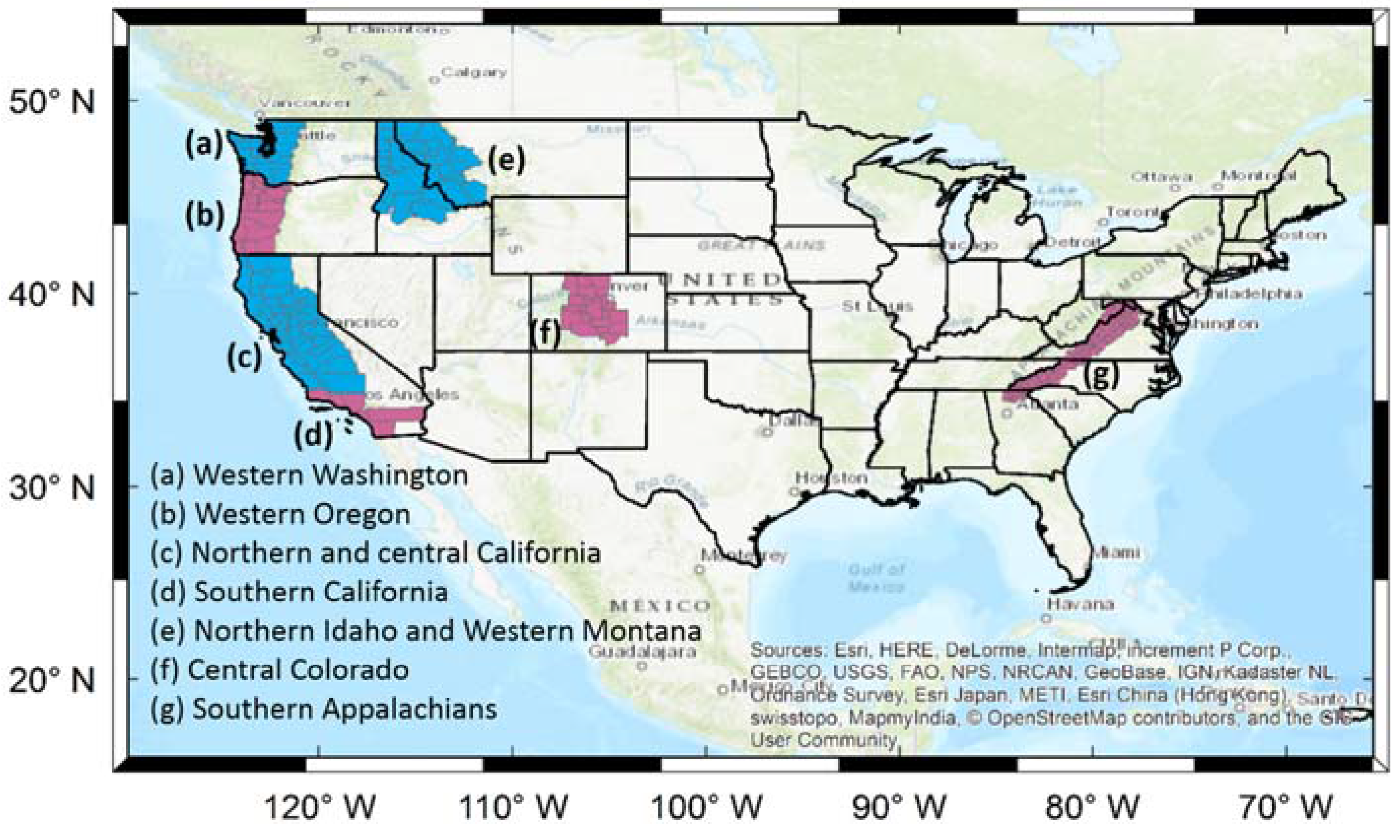
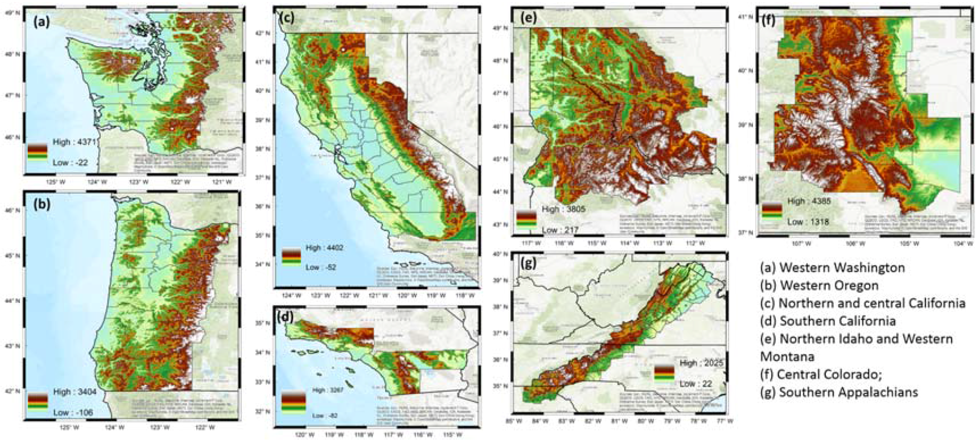
The selection criteria for study regions considered both terrain complexity and annual precipitation amounts. We picked study regions from major mountain ranges in the CONUS: the Appalachians, Rocky Mountains, Olympic Mountains, Pacific Coast Ranges, Cascade Range and Sierra Nevada. Each region was composed of multiple counties with complex terrain and relatively high annual precipitation. Four of the regions (Figure 1, Regions (a), (b), (c), and (d)) were along the Pacific coastline, where the climate is heavily influenced by the ocean and characterized by wet winters and dry summers. The other three (Figure 1, Regions (e), (f), and (g)) were inland regions with continental climates. Regional elevation maps are shown in Figure 2.
The Western Washington region (Figure 2a) covers the Olympic Mountains and the windward side of the North Cascade Range. The terrain has elevations ranging from 500 to 1500 m a.s.l. and several volcanoes reaching significantly higher altitudes than the rest of the mountains. This region is characterized by an oceanic climate with mild temperatures in all seasons. It has relatively dry summers, and most precipitation occurs in winter, spring and fall. The annual average precipitation varies roughly from 1500 to 3300 mm in higher altitude areas. On the western slopes of the Olympic Mountains, annual precipitation can exceed 4000 mm, which makes this region the rainiest in the CONUS.
The Western Oregon region (Figure 2b) is composed of the Pacific Coast Ranges, the windward side of the Central Cascade Range, the Northern Klamath Mountains and Willamette Valley. The elevations of most mountainous areas range from approximately 500 to 1500 m a.s.l. Like Western Washington, Western Oregon has an oceanic climate, with very wet winters and dry summers. The overall annual average precipitation in Western Oregon’s complex topography ranges between 1200 and 3000 mm, which is slightly lower than in Western Washington.
The study region of Northern and Central California (Figure 2c) covers the Southern Klamath Mountains, the Coast Ranges, the windward side of the Southern Cascade Range, the Sierra Nevada and the Great Valley. This region is characterized by extremely steep topographic gradients from the valleys to the mountains. The elevation ranges from approximately 400 to 2300 m a.s.l., while a small portion of the Sierra Nevada exceeds 3000 m a.s.l. Most of the precipitation occurs in mountainous areas. The northwestern part of this region has annual average precipitation between 1300 and 3000 mm, while other mountains in the region have less, ranging from 800 to 2300 mm.
The Southern California study region (Figure 2d) is smaller than the others. It includes the Peninsular Ranges and part of the Transverse Ranges. Elevations in most mountainous areas range from 200 to 2000 m a.s.l. Like the above three coastal regions, this region is under maritime influence, but the climate is much drier and hotter. Annual average precipitation ranges from approximately 200 to 700 mm.
The study region of Northern Idaho and Western Montana (Figure 2e) is an inland area covering part of the Middle Rocky Mountains. Elevation gradually increases from north to south and ranges roughly from 1000 to over 3800 m a.s.l. where Borah Peak is located. This region is dominated by a continental and subarctic climate with annual precipitation ranging from 500 to 1400 mm.
The Central Colorado region (Figure 2f) is located in the Southern Rocky Mountains. It is between the Continental Divide and western boundary of the Colorado Plains and includes Colorado’s most populated area (Front Range). The topography of most of this region is very complex, with elevations ranging between 1500 and 4300 m a.s.l. Similar to the Idaho and Montana region, Central Colorado has a continental or subarctic climate, but it has less precipitation. Annual average precipitation ranges between 350 and 800 mm.
The third inland region is located in the Southern Appalachians (Figure 2g). Specifically, it covers all of the Blue Ridge Mountains and part of the Ridge-and-Valley Appalachians, which are two physiographic provinces of the larger Appalachian range. Elevations of the mountainous areas range from approximately 500 to 1700 m a.s.l. Although it has a humid subtropical and temperate oceanic climate, we still count it as an inland region in this research because it includes no coastal area. Annual average precipitation ranges from 1000 to 2500 mm with no significant seasonal differences.
2.2. Precipitation Datasets
2.2.1. Satellite-Retrieved Product
The IMERG precipitation product is available at 0.1°/30-min resolution with quasi-global coverage (60°N–60°S). The IMERG algorithm merges all available satellite microwave precipitation estimates, the microwave-calibrated infrared (IR) satellite estimates, gauge analyses and other precipitation estimators from the TRMM and GPM eras [16]. In the GPM era (starting in 2014), IMERG is considered a more comprehensive precipitation product than those of the TRMM era (CMORPH, TRMM Multi-satellite Precipitation Analysis (TMPA), PERSIANN, GSMaP). In the consideration of observation data latencies, IMERG runs twice to provide quick estimates in near-real-time, which are the early run (~4-h latency, ftp://jsimpson.pps.eosdis.nasa.gov/data/imerg/early/) and late run (~12-h latency, ftp://jsimpson.pps.eosdis.nasa.gov/data/imerg/late/). After about 2.5 months, the IMERG final run (ftp://arthurhou.pps.eosdis.nasa.gov/gpmdata) provides a research-level product that is generated with more available satellite-based data and gauge data adjustment.
Since the research goal was to conduct near-real-time IMERG correction solely by the numerical weather prediction (NWP) model, an NWP-based adjustment was applied to the IMERG Version 5B Late run (~12-h latency) estimates (herein called raw IMERG-L). To compare the two adjustment methods—NWP-based and gauge-based—we also included the IMERG Version 5B Final run (~2.5-month latency) gauge-adjusted estimates (herein called gauge-adjusted IMERG-F) in the error analyses discussed in this paper.
2.2.2. Numerical Weather Prediction
We extracted precipitation forecasts from NCAR’s experimental real-time ensemble prediction system [34] (https://rda.ucar.edu/datasets/ds300.0/), which is a 10-member ensemble prediction system that produces daily 48-h forecasts with 3-km horizontal grid spacing over the CONUS using the Weather Research and Forecasting (WRF) model [35]. The ensemble data have been available since April 2015. All ensemble members share the same physics and dynamics, which makes them all equally likely to represent the “true” atmospheric state.
Schwartz et al. [34] evaluated the NCAR ensemble precipitation over the central and eastern CONUS and showed that the ensemble generally produced reasonable amplitudes of precipitation from the viewpoint of multi-month accumulation (7 April to 5 July 2015), while analyses of hourly precipitation rates revealed over-prediction at higher rates (≥5.0 mm/h) and under-prediction at lower rates. While Schwartz et al. [34] evaluated precipitation over an area with relatively lower elevation than the study domains in this research, Gowan et al. [36] found the NCAR ensemble performed well at high-altitude sites in the western United States. These collective results indicate that the NCAR ensemble precipitation was potentially suitable for conducting model-based correction on the underestimation of the raw IMERG-L product for heavy precipitation events in the case study areas.
2.2.3. NCEP Stage IV Product
For the reference precipitation data, we used the NCEP Stage IV precipitation dataset [23] (https://data.eol.ucar.edu/dataset/21.093), which is a multi-sensor (radar and gauge) product available over CONUS at approximately 4.7-km horizontal grid spacing. The final product is mosaicked by observations from twelve National Weather Service (NWS) River Forecast Centers (RFCs). Stage IV data are available in hourly, six-hourly and 24-hourly temporal resolutions. The six-hourly and 24-hourly products cover the entire CONUS, while the hourly product is not available in some of the western coastal states, where four of the coastal case study regions are located. Moreover, the hourly Stage IV product does not always include manual quality control from every RFC [37], but the six-hourly product does. Therefore, this study used the six-hourly product to evaluate the various precipitation estimates.
We note that Stage IV has less accuracy over the western mountainous states [37], where radar coverage is relatively sparse [38], and the corresponding RFCs use a unique rainfall processing algorithm named Mountain Mapper [39]. Nelson et al. [37] indicated underestimation in western RFC’s analysis data, which is due to the application of the Mountain Mapper algorithm. To quantify the underestimation, they showed bias ratios of Stage IV versus gauge data based on an 11-year period (2002 to 2012). The three western RFCs—Northwest, California-Nevada and Colorado basin—have seasonal bias ratios in the range of 0.78 to 0.82, 0.68 to 1.18 and 0.78 to 0.87, respectively. Consequently, the results of this paper may be affected by the Stage IV accuracy in western regions. Nevertheless, Stage IV is still used as reference data in this study because it is widely considered as the best gridded precipitation dataset over the CONUS.
3. Methodology
3.1. Event Selection
The precipitation events we selected occurred between May 2015 and December 2016 (a 20-month period). Since our research focused solely on flood-inducing storms, we first collected precipitation-caused flood reports from the NOAA Storm Events Database [40] for that period for each study region. We then identified precipitation events associated with these flood reports and eliminated coastal flood reports from the study because, precipitation aside, coastal flooding usually depends greatly on storm surge. We found a total of 523 precipitation-induced flood and flash flood reports for the seven study regions and study period, associated with 81 heavy precipitation events. The event lengths vary from 24 to 120 h. Although the NCAR ensemble provides daily 48-h forecasts, we only use the first 24-h forecasts for each event. In other words, events longer than 24 h employ the forecasts from two or more different model runs.
3.2. IMERG Adjustment
Before applying the model-based adjustment to raw IMERG-L, the hourly NCAR ensemble precipitation forecasts were summed to produce 6-hourly accumulations and upscaled from the original (3-km) grid to the 0.1° IMERG grid. We performed the remapping procedure by assigning model grid centers to each IMERG grid box. The average value of the NCAR model grid cells collocated with a particular IMERG grid box represented the remapped model value on the IMERG grid. We temporally aggregated the model and IMERG values at 6-hourly precipitation rates for consistency with the Stage IV temporal resolution.
We adjusted raw IMERG-L precipitation values by matching the raw IMERG-L precipitation quantiles with the model quantiles using a power-law function. Specifically, we computed precipitation quantile values from all non-zero, 6-hourly precipitation rates of each dataset. To simplify the calculation, we used only 5%, 10%, 15%, …, 95% quantile values in the data fitting equation shown below,
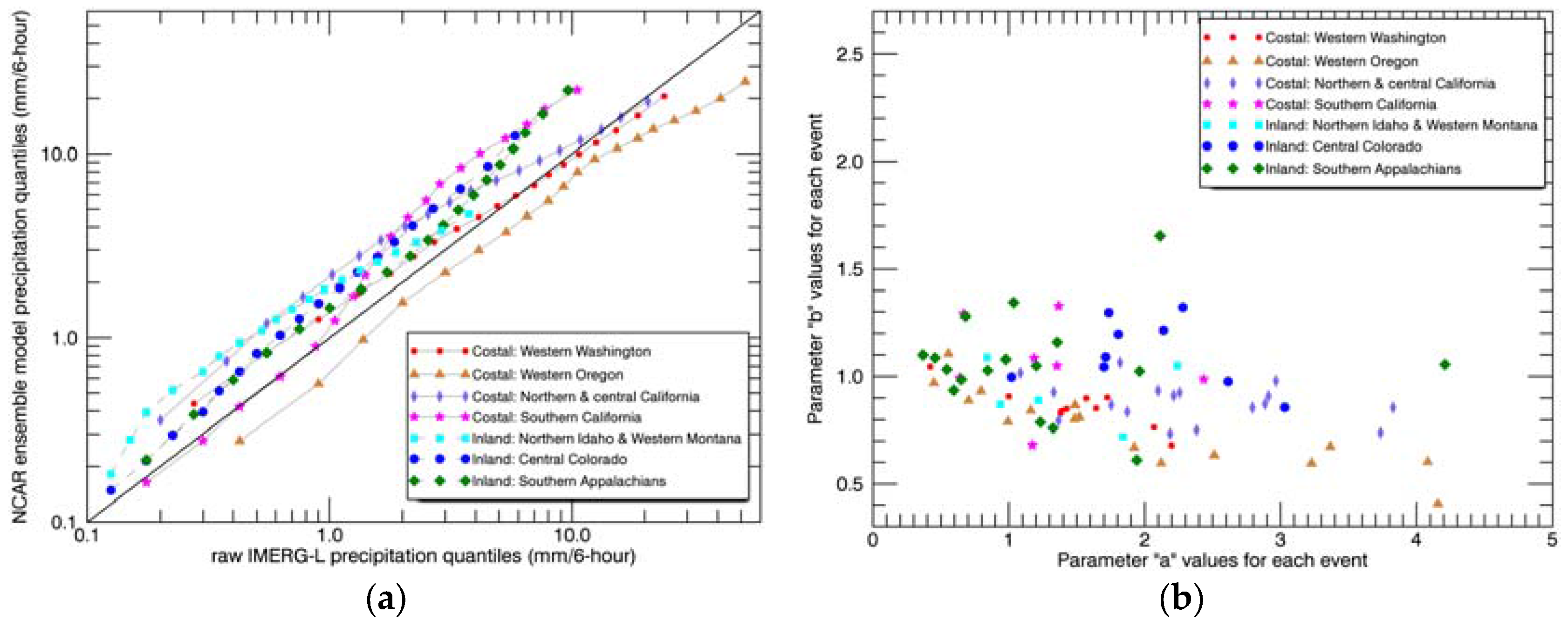
where X and Y represent the precipitation quantile values of raw IMERG-L and the model, respectively. We estimated the parameters a and b by the least squares method. The adjustment was done at the event scale, meaning a and b varied for each precipitation event. The quantile-quantile plot between raw IMERG-L and the mean of NCAR ensemble model products (Figure 3a) shows that the raw IMERG-L product has lower quantiles than the NCAR model in all study regions except Western Oregon. Further error analysis in Section 4.1 will show that the raw IMERG-L product underestimates over Western Oregon in terms of occurrence comparison at different precipitation thresholds, which is due to the fact that the NCAR model estimates precipitation more frequently than the satellite product. Figure 3b is a scatter plot of the values of parameters a and b for events in all regions. The parameter values from events occurring in the same region tend to be grouped together. Moreover, events in inland regions tend to have lower a values and higher b values, while events in coastal regions tend to have higher a values and lower b values. This indicates that the model-based adjustment performs differently for coastal and inland regions.
After data fitting, we applied the a and b values back to all raw IMERG-L precipitation rates by Equation 1 again to produce model-adjusted IMERG-L data. The adjustment can change the precipitation magnitude of the raw IMERG-L data, but cannot change the spatial pattern. Note that model precipitation is a 10-member ensemble dataset. Each member was used in the adjustment separately. Eventually, a new product was generated: model-adjusted IMERG-L ensemble precipitation.
3.3. Data Evaluation
We evaluated precipitation estimates for each event at 0.1° horizontal grid spacing, meaning we remapped Stage IV reference precipitation onto the IMERG grid by the same procedure we used for model remapping. We compared four estimators (model ensemble, raw IMERG-L, gauge-adjusted IMERG-F and model-adjusted IMERG-L ensemble precipitation) against the Stage IV reference precipitation at 6-hourly/0.1° grid spacing. The results shown below are based on median values of the model ensemble and the model-adjusted IMERG-L ensemble.
We quantitatively analyzed the 6-hourly precipitation rates using the Bias Ratio of frequency (BS), Heidke Skill Score (HSS) [41] and Critical Success Index (CSI). These error metrics are derived from the 2 × 2 contingency table representing the following four occurrence conditions:
- A is counted when estimator ≥ threshold and Stage IV ≥ threshold (hits);
- B is counted when estimator ≥ threshold and Stage IV < threshold (false alarms);
- C is counted when estimator < threshold and Stage IV ≥ threshold (misses);
- D is counted when estimator < threshold and Stage IV < threshold (correct rejections).
Each score is calculated at three thresholds. Threshold values varied for each region, depending on local precipitation intensity. The equation for BS is:
which shows an estimator’s bias for an entire study domain and a whole event, meaning BS is affected by the overall estimation, but not the exact location and timing of rainfall. It has a perfect value of 1, with below or above 1 representing under- or over-estimation, respectively.
The following equations are used to estimate the HSS:
PC is the percentage of correct estimates, and F is the fraction of correct estimates expected by chance. Finally, HSS is defined as the percentage of correct estimates that has been adjusted by the number expected to be correct by chance. Spatial mismatches in rainfall patterns would affect HSS performance and result in lower values. HSS values range from −∞ to 1, with 1 indicating a perfect set of estimation and negative values indicating that the given estimation has fewer hits (H) than a random estimation.
Finally, the CSI score is defined as:
CSI measures the fraction of precipitation rates that were correctly estimated. It examines the accuracy of the estimator without considering the correct rejections (D). CSI is sensitive to hits and penalized for misses and false alarms, so it is a function of Probability Of Detection (POD) and False Alarm Ratio (FAR). Unlike HSS, CSI is not affected by spatial mismatches in the rainfall patterns of different products, which means it can provide an evaluation for overall precipitation occurrences. The range of CSI values is from 0 to 1, with 1 as the perfect value.
To examine the performance of model-based IMERG adjustment in different topographic and climatic conditions, we classified the study regions into two groups: Pacific coastal regions and inland regions. Then, we analyzed the domain average event total precipitation estimation performance by the Pearson correlation coefficient (CORR) and normalized root-mean-square-error (NRMSE),
where n is number of events in each group and E and S are precipitation of the estimator and Stage IV, respectively. NRMSE measures the random component of error after removing the bias. CORR reveals the similarity of each estimator to Stage IV data.
4. Results and Discussion
4.1. Comparisons of Precipitation Rates
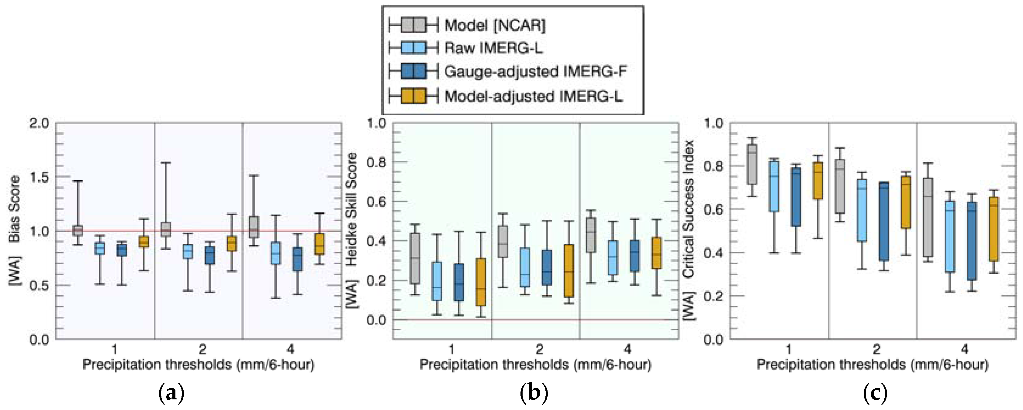
The seven study regions are discussed individually in this section. Figure 4 shows the error statistics of the six-hourly precipitation rate in the Western Washington region. The BS, HSS and CSI scores of all ten precipitation events occurring in this region are shown in boxplots, with three different rain rate thresholds for all estimators.
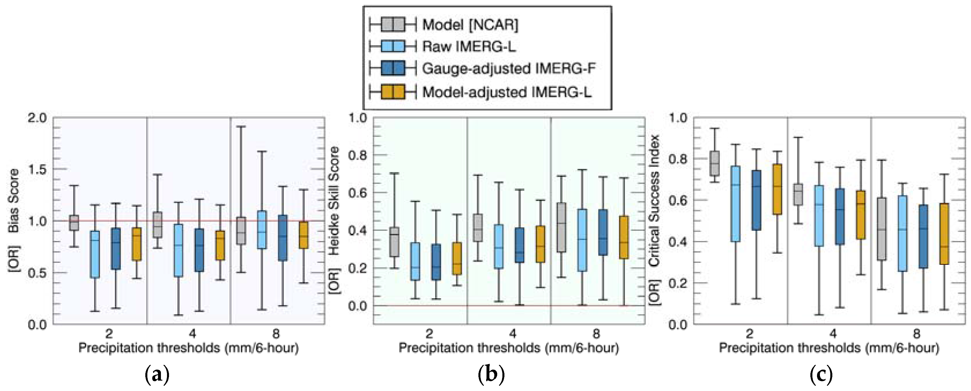
As the BS plot shows (Figure 4a), the raw IMERG-L product tended to underestimate the number of occurrences at all three precipitation thresholds, while the model data tended toward slight overestimation. The gauge-based adjustment did not improve IMERG performance; in fact, it enhanced the underestimation. In contrast, the model-adjusted IMERG-L product showed considerable improvement, with BS values much closer to one for all precipitation thresholds.
HSS values (Figure 4b) showed that model forecasts exhibited higher scores than the IMERG estimates for all thresholds, and the raw IMERG-L score was relatively low. The performances of the gauge-adjusted IMERG-F and model-adjusted IMERG-L products were similar to that of the raw IMERG-L. This result indicated that neither IMERG adjustment could reduce the random component of the error.
The CSI values (Figure 4c) for all estimators decreased as the rainfall threshold increased. Although the CSI values of the raw IMERG-L and gauge-adjusted IMERG-F products were relatively low, the model-adjusted IMERG-L product produced higher values, indicating that the model-based adjustment effectively increased the percentage of correct estimates. Overall, the model-adjusted IMERG-L performed better than all three IMERG-related products, although the NCAR model forecast provided an even better estimation.
Figure 5 shows the results of the analysis of 16 heavy precipitation events in the Western Oregon region. The raw IMERG-L exhibited underestimation (Figure 5a). While the model-based adjustment effectively moderated the negative biases, the gauge-based adjustment had no impact on the raw IMERG-L product. In fact, the gauge-adjusted IMERG-F showed no improvement for any error metric (BS, HSS or CSI). Meanwhile, the model forecast was consistently superior to the three IMERG products at lower precipitation thresholds (2 and 4 mm/6 h) for all error metrics, while at the high threshold (8 mm/6 h), the performance of the model-adjusted IMERG-L was comparable to that of the model forecast.
Results for the North and Central California region (Figure 6) were based on 17 heavy precipitation events. BS values of the raw IMERG-L product continued to exhibit severe underestimation (Figure 6a). Unlike in the Washington and Oregon regions, the gauge-based adjustment in this region did improve the precipitation estimates. Meanwhile, the model-based adjustment performed even better, especially at the 8 mm/6 h threshold, where the median BS value was very close to one. The advantage of model-based adjustment could also be found in the HSS and CSI (Figure 6b,c). Overall, the model-adjusted IMERG-L had not only higher HSS and CSI median values, but also narrower score value ranges than the other two IMERG products. Still, although the model-adjusted IMERG-L proved superior to the other IMERG products, the model forecast showed the overall best performance for all error metrics in this region.
Southern California (Figure 7) is the last coastal study region discussed here. Given the relatively dry climatic conditions of this area, only seven flood-inducing precipitation events were identified. Similar to the above three coastal regions, the raw IMERG-L product was shown to be the least accurate estimator, with apparent underestimations (Figure 7a), and the model forecast performed the best for all error metrics. Nevertheless, unique to this region was the slightly better performance of the gauge-based adjustment relative to that of the model-based adjustment for BS, HSS and CSI, even though both adjustments appeared to be more accurate than the raw IMERG-L. Moreover, the comparison of BS plots across all four coastal regions showed Southern California with the greatest raw IMERG-L underestimation, and the two adjustment methods were unable to improve IMERG to a reasonable level.
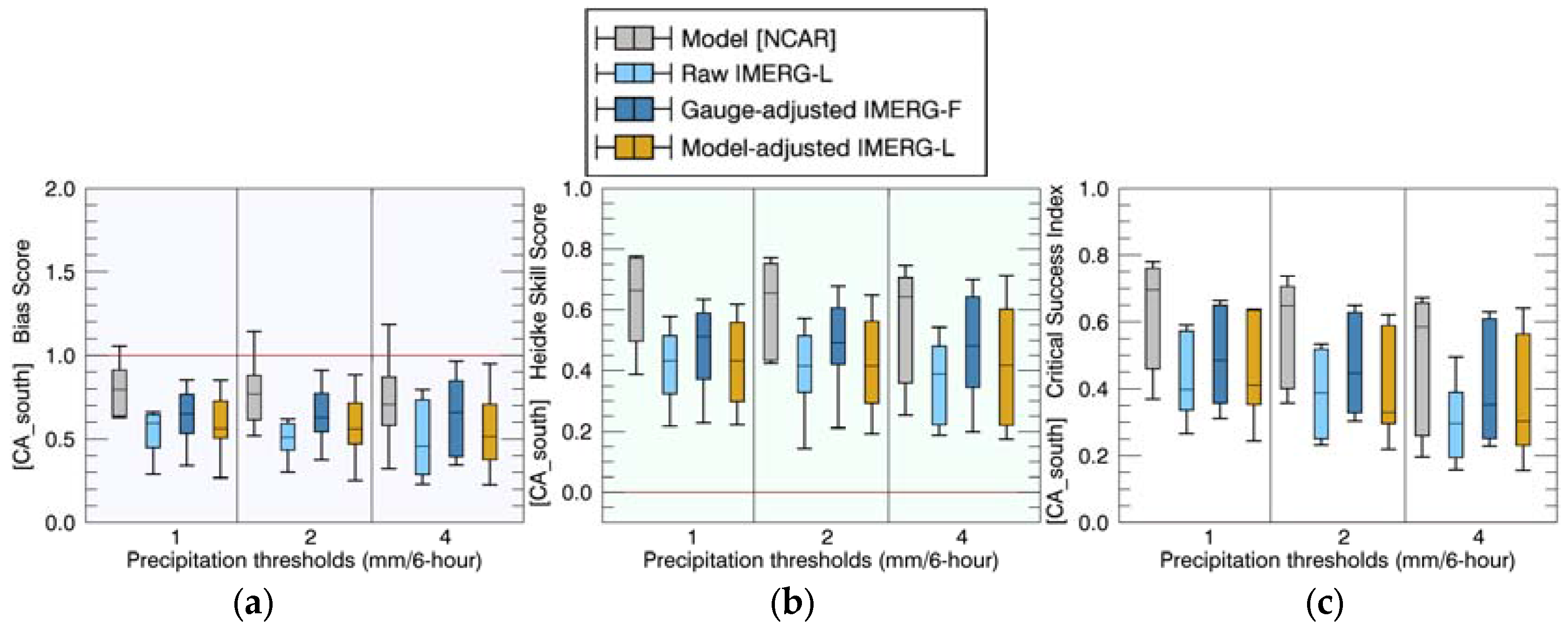
With regards to inland areas, five flood-inducing precipitation events were included in the error metrics for the Northern Idaho and Western Montana region (Figure 8). The raw IMERG-L product exhibited underestimation, and the model forecast had BS values mostly around one (Figure 8a). At the 1 and 2 mm/6 h thresholds, the gauge-based adjustment shrank the BS range, but the median BS values remained similar, indicating no improvement, while the model-adjusted IMERG-L product exhibited substantial improvement. At the 4 mm/6 h threshold, the gauge-adjusted IMERG-F increased BS values, but still had a wide value range, while model-adjusted IMERG-L exhibited underestimation, but with a narrower value range. HSS and CSI plots (Figure 8b,c) showed similar error characteristics in the comparison among the four estimators. Basically, the two adjusted IMERG products performed comparably to the model forecast at high thresholds and were less accurate at lower thresholds.
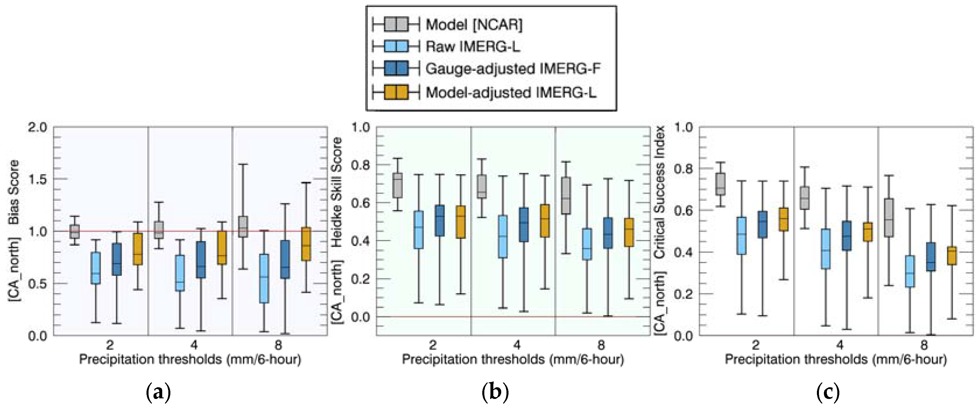
The Central Colorado region had nine precipitation events included in the analysis (Figure 9). As in all the above regions, the raw IMERG-L showed severe underestimation for all rain rate thresholds (Figure 9a). Gauge-based adjustment had very limited impact on the IMERG product; thus, the error scores showed no substantial improvement. Comparison of the BS, HSS and CSI metrics indicated that the model-adjusted IMERG-L product was superior to any of the other estimators, including the model forecast. In fact, the model forecast in this region had a general trend of overestimation and relatively low performance in terms of HSS and CSI values.
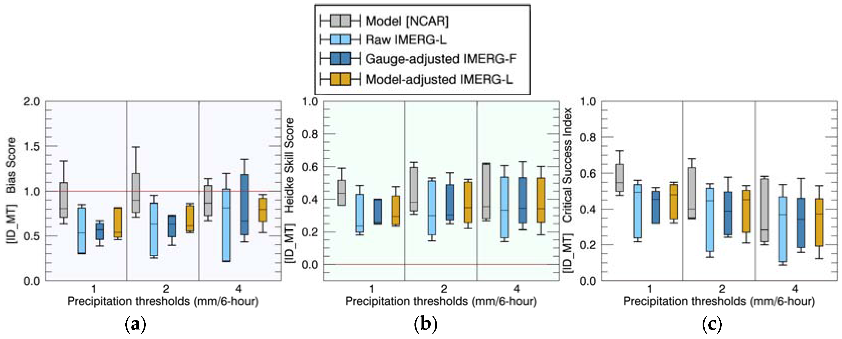
Seventeen precipitation events were analyzed in the Southern Appalachians region (Figure 10), with results similar to those for the Colorado region; the raw IMERG-L tended to underestimate for all rain rate thresholds, and the model-adjusted product had the best HSS and CSI (Figure 10b,c). The BS of the model forecast was comparable to that of the model-adjusted IMERG-L (Figure 10a). A possible explanation for the disagreement between the HSS/CSI and BS scores is that the model successfully predicted the domain average rainfall intensity, but with the wrong spatial patterns.
Overall, for all study regions, the raw IMERG-L product exhibited the poorest performance of rain rate estimation. Both model- and gauge-based adjustments reflected the effectiveness of IMERG correction. Table 1 compares the two adjustments over coastal regions in terms of the number of events that are improved, exhibit no change or worsened by the adjustments. The model-based adjustment outperforms the gauge-based adjustment with BS and CSI, but not with HSS. Over inland regions (Table 2), IMERG-L benefited more from model-based adjustment than from gauge-based adjustment for all statistical scores. The best-performing product varied under different topographic and climatic conditions. In coastal regions, the model forecast was superior to the two adjusted IMERG (IMERG-F and model-adjusted IMERG-L) products, especially for lower rain rates, while the performance of these products was better than or comparable to that of the model forecast over inland regions.
4.2. Comparisons of Event Total Precipitation
To illustrate the spatial rainfall distribution of each dataset, we show event total precipitation maps for three events (Figure 11). First, the typical characteristics of each product in coastal regions are shown by a 42-h event that occurred in Northern and Central California, beginning on 15 October 2016, at 18:00 UTC (Figure 11, top row). Taking the Stage IV product as a reference, the model forecast captured all major rain bands in this area with reasonable magnitude, which supports the finding that the model had the best performance in rain rate error metrics over coastal regions. Although the raw IMERG-L product had severe underestimation, it accurately captured the northwestern rain band. Meanwhile, the rain band in the Sierra Nevada was not captured correctly. The model-based adjustment was effective in dealing with the underestimation of precipitation over the northwestern corner, but it could not improve the estimation for Sierra Nevada because the adjustment is sensitive only to magnitude correction. The gauge-adjusted IMERG-F product did not show enough improvement, either.
The second event occurred in central Colorado on 7 May 2015, at 18:00 UTC, and lasted for three days (Figure 11, middle row). The model prediction was fairly accurate with regard to the overall rainfall magnitude, but the most intense precipitation was erroneously located at the northeastern corner of the domain, while Stage IV showed intense rain over the southeastern part. In contrast, although the raw IMERG-L product largely underestimated the rainfall magnitude, it captured the correct location of the intense rain. After the model-based adjustment, the IMERG-L product achieved the best estimation of the four estimators.
The model precipitation location issue arose in the Southern Appalachians, as well (Figure 11, bottom row). This was a two-day event starting on 29 September 2016, at 00:00 UTC. As with the Colorado event, the model predicted rainfall intensity well from the domain average perspective, but with the wrong spatial distribution of precipitation. The raw IMERG-L product showed severe underestimation again, but with correct spatial distribution of precipitation. The model-adjusted IMERG-L product had the best performance, taking advantage of rainfall intensity from the model and spatial distribution from the raw IMERG-L.
Statistics for the domain-average event-total precipitation validated the findings from the rain maps (Table 3). We classified the mountainous heavy precipitation events into two groups: coastal region (50 events) and inland region (31 events). Then, we calculated the CORR and NRMSE with respect to reference Stage IV data. The raw IMERG-L product exhibited the lowest CORR and the highest NRMSE for both the coastal and inland regions. The two IMERG adjustment methods effectively improved the pure satellite product. Comparison between the two methods showed that the model-based adjustment was always superior to the gauge-based adjustment, with the exception of coastal region CORR, for which the performance was the same. Taking model forecast data into account, the model performed better than the model-adjusted IMERG-L product for coastal region events. For inland region events, however, the model-adjusted IMERG-L was more accurate than the model itself. This may be due to the fact that the model tended to erroneously place intense precipitation over inland regions, while the raw IMERG-L product was more likely to have difficulty capturing rain band structures over coastal regions, but generally showed correct spatial distributions over inland regions.
4.3. Discussion: Comparison to Previous Studies
The technique of model-based satellite adjustment was first introduced by Zhang et al. [29] and demonstrated on five heavy precipitation events over the European Alps and Massif Central. The raw CMORPH product largely underestimated high rain rates, while the WRF simulations provided reasonable overall rainfall magnitudes. Results based on the limited storms from that study showed that the technique efficiently reduced the underestimation of high rain rates, thus providing an improved product.
After the successful first attempt in middle-latitude regions, a more comprehensive study examined the technique in three tropical mountainous regions (Colombian Andes, Peruvian Andes and Taiwan) from 81 storm cases [33]. The raw and gauge-adjusted CMORPH and GSMaP products were involved. As expected, raw CMORPH and GSMaP exhibited severe underestimation in all regions, and the bias was more significant at higher rain rates. Improvements of gauge-based adjustment were shown to be limited, possibly due to the sparse gauge network incorporated in the satellite adjustment. Meanwhile, WRF model-adjusted products outperformed either the gauge-based adjustments or the WRF model itself. The adjustments for higher rain rates were more effective than low rain rates.
Aside from the above mid- and low-latitude applications, there were two studies focusing on CONUS mountain ranges. One of them examined six extreme events induced by hurricane landfalls in the Southern Appalachians [32]. Again, raw CMORPH underestimated all events. Improvements were comparable between WRF model- and gauge-adjusted products. In order to evaluate the impact of satellite adjustment on flood simulations, a hydrological model ran for 20 basins over the study region and showed considerable improvements on the runoff outputs simulated by adjusted CMORPH products.
Nikolopoulos et al. [31] focused on a single extreme rainfall event that occurred in September 2013, in Colorado. Model forecasts produced by the Regional Atmospheric Modeling System and Integrated Community Limited Area Modeling System (RAMS-ICLAMS) were utilized to adjust raw CMORPH, TRMM 3B42RT and weather radar (Multi-Radar Multi-Sensor (MRMS)) estimates. The adjustments were applied by two different procedures: (i) mean field bias and (ii) the adjustment technique herein. Both procedures provided improvements to raw satellite and radar products, with the latter one performing better in terms of random error and correlation.
These previous studies have focused on products during the TRMM era. In the GPM era, the new IMERG products are expected to be extensively used in many applications. In addition, an important gap in past studies was the use of NWP analysis (with the exception of [31]) vs. forecasts that is needed for applications with near-real-time IMERG products. The current study used the NCAR real-time ensemble forecasts for this purpose and demonstrated improvements based on a large number of flash flood events over complex terrain areas in the CONUS. We are encouraged by the results that the model-based adjustment technique can provide improvements to the state-of-the-art IMERG products, especially by the fact that the model-adjusted product outperformed the gauge-adjusted one, which is consistent with the findings of previous studies applied to CMORPH and GSMaP across global mountainous areas.
Combining our studies so far, the technique of model-based satellite precipitation adjustment has been examined over mountainous areas around the world with different terrain complexity and climatic conditions. Results show that the model-adjusted products outperform, or at least are comparable to, the gauge-adjusted products for all high-resolution satellite datasets examined. Moreover, the model-based adjustment requires no gauge network and much less processing time. The results are promising for future applications of model-based satellite precipitation adjustment over mountainous areas, especially for areas lacking ground observations. To successfully apply the technique, there are two prerequisites: (i) the raw satellite data capture the relative spatial and temporal variabilities of precipitation (i.e., no significant surface contamination effects on satellite precipitation detection); and (ii) the model provides relatively accurate precipitation outputs in terms of overall magnitude (not necessarily location).
5. Conclusions
The primary objectives of this study were, first, to examine the feasibility of an ensemble model-based IMERG adjustment technique and, second, to compare the performances of the model-adjusted IMERG-L, a gauge-adjusted IMERG-F and the model itself. Major conclusions are summarized below.
The raw IMERG-L product consistently underestimated heavy precipitation in all study regions over the CONUS, while the rainfall magnitudes exhibited in the NCAR real-time model forecast were fairly accurate. From the perspective of spatial distribution, the raw IMERG-L product was more likely to have difficulty capturing rain band structures over coastal regions, but generally showed correct spatial distributions over inland regions. On the other hand, the model tended to erroneously place intense precipitation over inland regions.
In general, the model-based adjustment could successfully increase the raw IMERG-L precipitation magnitude without changing its spatial pattern and, ultimately, provided a more accurate product than the raw product. While the IMERG-F product could benefit from gauge-based adjustment, as well, the improvement from model-based adjustment was consistently more significant, except in the Southern California region. Comparison between the model forecast and the model-adjusted IMERG-L product showed that the former performed even better than the latter for coastal region events. For inland events, however, the model-adjusted IMERG-L was more accurate than the model itself.
As described in the IMERG technical document [16], the final gauge-adjusted IMERG-F product usually has a 2.5-month latency before it is publicly available. On the other hand, the model-adjusted IMERG-L precipitation can be produced concurrently with the raw IMERG-L, as it requires no gauge observations and is based on NWP model forecasts. Moreover, given that the model-adjusted IMERG-L product performs consistently better than its gauge-adjusted counterpart, it is safe to conclude that model-based adjustment is a feasible technique to improve the quality of the near-real-time IMERG-L product for mountainous heavy precipitation events.
Since the precipitation events in this research were all flood-inducing storms, future studies can focus on the hydrological processes of related flood events. The three IMERG products analyzed here can be used to force a hydrological model and simulate runoff for corresponding basins to evaluate error propagation.
Acknowledgments
Glen Romine, Kate Fossell and Ryan Sobash are thanked for their efforts to produce the NCAR ensemble forecasts. NCAR is sponsored by the National Science Foundation. Xinxuan Zhang was funded by the Eversource Energy Center at the University of Connecticut.
Author Contributions
Xinxuan Zhang and Emmanouil N. Anagnostou conceived of and designed the model-based satellite precipitation adjustment. Xinxuan Zhang performed the adjustment and analyzed the data. Craig S. Schwartz contributed the NCAR ensemble forecast data. Xinxuan Zhang wrote the paper. Emmanouil Anagnostou and Craig Schwartz contributed to the writing of the paper.
Conflicts of Interest
The authors declare no conflict of interest. The founding sponsors had no role in the design of the study; in the collection, analyses or interpretation of data; in the writing of the manuscript; nor in the decision to publish the results.
References
- Roe, G.H. Orographic precipitation. Annu. Rev. Earth Planet. Sci. 2005, 33, 645–671. [Google Scholar] [CrossRef]
- Houze, R.A. Orographic effects on precipitating clouds. Rev. Geophys. 2012, 50. [Google Scholar] [CrossRef]
- Becker, A.; Finger, P.; Meyer-Christoffer, A.; Rudolf, B.; Schamm, K.; Schneider, U.; Ziese, M. A description of the global land-surface precipitation data products of the Global Precipitation Climatology Centre with sample applications including centennial (trend) analysis from 1901–present. Earth Syst. Sci. Data 2013, 5, 71–99. [Google Scholar] [CrossRef]
- Schamm, K.; Ziese, M.; Becker, A.; Finger, P.; Meyer-Christoffer, A.; Schneider, U.; Schröder, M.; Stender, P. Global gridded precipitation over land: A description of the new GPCC First Guess Daily product. Earth Syst. Sci. Data 2014, 6, 49–60. [Google Scholar] [CrossRef]
- Haylock, M.R.; Hofstra, N.; Klein Tank, A.M.G.; Klok, E.J.; Jones, P.D.; New, M. A European daily high-resolution gridded data set of surface temperature and precipitation for 1950–2006. J. Geophys. Res. 2008, 113. [Google Scholar] [CrossRef]
- Yatagai, A.; Arakawa, O.; Kamiguchi, K.; Kawamoto, H.; Nodzu, M.I.; Hamada, A. A 44-year daily gridded precipitation dataset for Asia based on a dense network of rain gauges. Sola 2009, 5, 137–140. [Google Scholar] [CrossRef]
- Krajewski, W.F.; Smith, J.A. Radar hydrology: Rainfall estimation. Adv. Water Resour. 2002, 25, 1387–1394. [Google Scholar] [CrossRef]
- Germann, U.; Galli, G.; Boscacci, M.; Bolliger, M. Radar precipitation measurement in a mountainous region. Q. J. R. Meteorol. Soc. 2006, 132, 1669–1692. [Google Scholar] [CrossRef]
- Villarini, G.; Krajewski, W.F. Review of the different sources of uncertainty in single polarization radar-based estimates of rainfall. Surv. Geophys. 2010, 31, 107–129. [Google Scholar] [CrossRef]
- Kidd, C.; Levizzani, V. Status of satellite precipitation retrievals. Hydrol. Earth Syst. Sci. 2011, 15, 1109–1116. [Google Scholar] [CrossRef] [Green Version]
- Huffman, G.J.; Bolvin, D.T.; Nelkin, E.J.; Wolff, D.B.; Adler, R.F.; Gu, G.; Hong, Y.; Bowman, K.P.; Stocker, E.F. The TRMM multisatellite precipitation analysis (TMPA): Quasi-global, multiyear, combined-sensor precipitation estimates at fine scales. J. Hydrometeorol. 2007, 8, 38–55. [Google Scholar] [CrossRef]
- Joyce, R.J.; Janowiak, J.E.; Arkin, P.A.; Xie, P. CMORPH: A method that produces global precipitation estimates from passive microwave and infrared data at high spatial and temporal resolution. J. Hydrometeorol. 2004, 5, 487–503. [Google Scholar] [CrossRef]
- Sorooshian, S.; Hsu, K.L.; Gao, X.; Gupta, H.V.; Imam, B.; Braithwaite, D. Evaluation of PERSIANN system satellite–based estimates of tropical rainfall. Bull. Am. Meteorol. Soc. 2000, 81, 2035–2046. [Google Scholar] [CrossRef]
- Kubota, T.; Shige, S.; Hashizume, H.; Aonashi, K.; Takahashi, N.; Seto, S.; Takayabu, Y.N.; Ushio, T.; Nakagawa, K.; Iwanami, K. Global precipitation map using satellite-borne microwave radiometers by the GSMaP project: Production and validation. IEEE Trans. Geosci. Remote Sens. 2007, 45, 2259–2275. [Google Scholar] [CrossRef]
- Ushio, T.; Sasashige, K.; Kubota, T.; Shige, S.; Okamoto, K.; Aonashi, K.; Inoue, T.; Takahashi, N.; Iguchi, T.; Kachi, M. A Kalman filter approach to the Global Satellite Mapping of Precipitation (GSMaP) from combined passive microwave and infrared radiometric data. J. Meteorol. Soc. Jpn. Ser. II 2009, 87, 137–151. [Google Scholar] [CrossRef]
- Huffman, G.J.; Bolvin, D.T.; Braithwaite, D.; Hsu, K.; Joyce, R.; Kidd, C.; Nelkin, E.J.; Sorooshian, S.; Tan, J.; Xie, P. NASA global precipitation measurement (GPM) integrated multi-satellite retrievals for GPM (IMERG). In Algorithm Theoretical Basis Document, version 5.1; National Aeronautics and Space Administration: Washington, DC, USA, 2017. [Google Scholar]
- Hirpa, F.A.; Gebremichael, M.; Hopson, T. Evaluation of high-resolution satellite precipitation products over very complex terrain in Ethiopia. J. Appl. Meteorol. Climatol. 2010, 49, 1044–1051. [Google Scholar] [CrossRef]
- Gao, Y.C.; Liu, M. Evaluation of high-resolution satellite precipitation products using rain gauge observations over the Tibetan Plateau. Hydrol. Earth Syst. Sci. 2013, 17, 837. [Google Scholar] [CrossRef]
- Stampoulis, D.; Anagnostou, E.N.; Nikolopoulos, E.I. Assessment of high-resolution satellite-based rainfall estimates over the Mediterranean during heavy precipitation events. J. Hydrometeorol. 2013, 14, 1500–1514. [Google Scholar] [CrossRef]
- Derin, Y.; Anagnostou, E.; Berne, A.; Borga, M.; Boudevillain, B.; Buytaert, W.; Chang, C.-H.; Delrieu, G.; Hong, Y.; Hsu, Y.C. Multiregional satellite precipitation products evaluation over complex terrain. J. Hydrometeorol. 2016, 17, 1817–1836. [Google Scholar] [CrossRef]
- Maggioni, V.; Meyers, P.C.; Robinson, M.D. A review of merged high-resolution satellite precipitation product accuracy during the Tropical Rainfall Measuring Mission (TRMM) era. J. Hydrometeorol. 2016, 17, 1101–1117. [Google Scholar] [CrossRef]
- Beck, H.E.; Vergopolan, N.; Pan, M.; Levizzani, V.; van Dijk, A.I.; Weedon, G.P.; Brocca, L.; Pappenberger, F.; Huffman, G.J.; Wood, E.F. Global-scale evaluation of 22 precipitation datasets using gauge observations and hydrological modeling. Hydrol. Earth Syst. Sci. 2017, 21, 6201. [Google Scholar] [CrossRef]
- Lin, Y.; Mitchell, K.E. The NCEP stage II/IV hourly precipitation analyses: Development and applications. In Proceedings of the 19th Conf. Hydrology, San Diego, CA, USA, 9–13 January 2005. [Google Scholar]
- Sinclair, S.; Pegram, G. Combining radar and rain gauge rainfall estimates using conditional merging. Atmos. Sci. Lett. 2005, 6, 19–22. [Google Scholar] [CrossRef]
- Goudenhoofdt, E.; Delobbe, L. Evaluation of radar-gauge merging methods for quantitative precipitation estimates. Hydrol. Earth Syst. Sci. 2009, 13, 195–203. [Google Scholar] [CrossRef]
- Mega, T.; Ushio, T.; Kubota, T.; Kachi, M.; Aonashi, K.; Shige, S. Gauge adjusted global satellite mapping of precipitation (GSMaP_Gauge). In Proceedings of the 2014 XXXIth URSI General Assembly and Scientific Symposium (URSI GASS), Beijing, China, 16–23 August 2014; pp. 1–4. [Google Scholar] [CrossRef]
- Xie, P.; Yoo, S.-H.; Joyce, R.; Yarosh, Y. Bias-corrected CMORPH: A 13-year analysis of high-resolution global precipitation. Geophys. Res. Abstr. 2011, 13. Abstract EGU2011-1809. [Google Scholar]
- Xie, P.; Joyce, R.; Wu, S.; Yoo, S.-H.; Yarosh, Y.; Sun, F.; Lin, R. Reprocessed, bias-corrected CMORPH global high-resolution precipitation estimates from 1998. J. Hydrometeorol. 2017, 18, 1617–1641. [Google Scholar] [CrossRef]
- Zhang, X.; Anagnostou, E.N.; Frediani, M.; Solomos, S.; Kallos, G. Using NWP simulations in satellite rainfall estimation of heavy precipitation events over mountainous areas. J. Hydrometeorol. 2013, 14, 1844–1858. [Google Scholar] [CrossRef]
- Scofield, R.A.; Kuligowski, R.J. Status and outlook of operational satellite precipitation algorithms for extreme-precipitation events. Weather Forecast. 2003, 18, 1037–1051. [Google Scholar] [CrossRef]
- Nikolopoulos, E.I.; Bartsotas, N.S.; Anagnostou, E.N.; Kallos, G. Using high-resolution numerical weather forecasts to improve remotely sensed rainfall estimates: The case of the 2013 Colorado flash flood. J. Hydrometeorol. 2015, 16, 1742–1751. [Google Scholar] [CrossRef]
- Zhang, X.; Anagnostou, E.N.; Vergara, H. Hydrologic Evaluation of NWP-Adjusted CMORPH Estimates of Hurricane-Induced Precipitation in the Southern Appalachians. J. Hydrometeorol. 2016, 17, 1087–1099. [Google Scholar] [CrossRef]
- Zhang, X.; Anagnostou, E.N. Evaluation of Numerical Weather Model-based Satellite Precipitation Adjustment in Tropical Mountainous Regions. J. Hydrometeorol. 2018. under review. [Google Scholar]
- Schwartz, C.S.; Romine, G.S.; Sobash, R.A.; Fossell, K.R.; Weisman, M.L. NCAR’s experimental real-time convection-allowing ensemble prediction system. Weather Forecast. 2015, 30, 1645–1654. [Google Scholar] [CrossRef]
- Skamarock, W.C.; Klemp, J.B.; Dudhia, J.; Gill, D.O.; Barker, D.M.; Duda, M.G.; Huang, X.; Wang, W.; Powers, J.G. A Description of the Advanced Research WRF, version 3; NCAR Technical Note; NCAR/TN-475+ STR; National Center for Atmospheric Research: Boulder, CO, USA, 2008. [Google Scholar]
- Gowan, T.M.; Steenburgh, W.J.; Schwartz, C.S. Validation of mountain precipitation forecasts from the convection-permitting NCAR Ensemble and operational forecast systems over the Western United States. Weather Forecast. 2018, in press. [Google Scholar] [CrossRef]
- Nelson, B.R.; Prat, O.P.; Seo, D.-J.; Habib, E. Assessment and implications of NCEP stage IV quantitative precipitation estimates for product intercomparisons. Weather Forecast. 2016, 31, 371–394. [Google Scholar] [CrossRef]
- Maddox, R.A.; Zhang, J.; Gourley, J.J.; Howard, K.W. Weather radar coverage over the contiguous United States. Weather Forecast. 2002, 17, 927–934. [Google Scholar] [CrossRef]
- Hou, D.; Charles, M.; Luo, Y.; Toth, Z.; Zhu, Y.; Krzysztofowicz, R.; Lin, Y.; Xie, P.; Seo, D.-J.; Pena, M. Climatology-calibrated precipitation analysis at fine scales: Statistical adjustment of stage IV toward CPC gauge-based analysis. J. Hydrometeorol. 2014, 15, 2542–2557. [Google Scholar] [CrossRef]
- NOAA Storm Events Database. Available online: https://www.ncdc.noaa.gov/stormevents/ (accessed on 20 February 2018).
- Heidke, P. Berechnung des Erfolges und der Güte der Windstärkevorhersagen im Sturmwarnungsdienst. Geogr. Ann. 1926, 8, 301–349. [Google Scholar] [CrossRef]
Figure 1.
Location of the seven study regions over the conterminous United States (CONUS).

Figure 2.
Map of terrain elevation for the seven study regions (meters). DEM data are from the USGS Shuttle Radar Topography Mission (SRTM, https://lta.cr.usgs.gov/SRTM). Data are available at https://dds.cr.usgs.gov/srtm/version2_1/SRTM3/North_America/.
Figure 2.
Map of terrain elevation for the seven study regions (meters). DEM data are from the USGS Shuttle Radar Topography Mission (SRTM, https://lta.cr.usgs.gov/SRTM). Data are available at https://dds.cr.usgs.gov/srtm/version2_1/SRTM3/North_America/.

Figure 3.
(a) Quantile-quantile plot of the raw IMERG-L (Late run) product vs. the NCAR model product; (b) scatter plot of the values of parameters a and b for events in all regions.
Figure 3.
(a) Quantile-quantile plot of the raw IMERG-L (Late run) product vs. the NCAR model product; (b) scatter plot of the values of parameters a and b for events in all regions.

Figure 4.
Error statistics of precipitation rate in Western Washington Region. (a) Bias Ratio of frequency (BS), (b) Heidke Skill Score (HSS) and (c) Critical Success Index (CSI).
Figure 4.
Error statistics of precipitation rate in Western Washington Region. (a) Bias Ratio of frequency (BS), (b) Heidke Skill Score (HSS) and (c) Critical Success Index (CSI).

Figure 5.
Error statistics of precipitation rate in Western Oregon Region. (a) Bias Ratio of frequency (BS), (b) Heidke Skill Score (HSS) and (c) Critical Success Index (CSI).
Figure 5.
Error statistics of precipitation rate in Western Oregon Region. (a) Bias Ratio of frequency (BS), (b) Heidke Skill Score (HSS) and (c) Critical Success Index (CSI).

Figure 6.
Error statistics of precipitation rate in Northern and Central California Region. (a) Bias Ratio of frequency (BS), (b) Heidke Skill Score (HSS) and (c) Critical Success Index (CSI).
Figure 6.
Error statistics of precipitation rate in Northern and Central California Region. (a) Bias Ratio of frequency (BS), (b) Heidke Skill Score (HSS) and (c) Critical Success Index (CSI).

Figure 7.
Error statistics of precipitation rate in Southern California Region. (a) Bias Ratio of frequency (BS), (b) Heidke Skill Score (HSS) and (c) Critical Success Index (CSI).
Figure 7.
Error statistics of precipitation rate in Southern California Region. (a) Bias Ratio of frequency (BS), (b) Heidke Skill Score (HSS) and (c) Critical Success Index (CSI).

Figure 8.
Error statistics of precipitation rate in Northern Idaho and Western Montana Region. (a) Bias Ratio of frequency (BS), (b) Heidke Skill Score (HSS) and (c) Critical Success Index (CSI).
Figure 8.
Error statistics of precipitation rate in Northern Idaho and Western Montana Region. (a) Bias Ratio of frequency (BS), (b) Heidke Skill Score (HSS) and (c) Critical Success Index (CSI).

Figure 9.
Error statistics of precipitation rate in Central Colorado Region. (a) Bias Ratio of frequency (BS), (b) Heidke Skill Score (HSS) and (c) Critical Success Index (CSI).
Figure 9.
Error statistics of precipitation rate in Central Colorado Region. (a) Bias Ratio of frequency (BS), (b) Heidke Skill Score (HSS) and (c) Critical Success Index (CSI).

Figure 10.
Error statistics of precipitation rate in Southern Appalachians Regions. (a) Bias Ratio of frequency (BS), (b) Heidke Skill Score (HSS) and (c) Critical Success Index (CSI).
Figure 10.
Error statistics of precipitation rate in Southern Appalachians Regions. (a) Bias Ratio of frequency (BS), (b) Heidke Skill Score (HSS) and (c) Critical Success Index (CSI).

Figure 11.
Event total precipitation maps for selected storms. Top panel: event in Northern and Central California (start at 15 October 2016 18:00 UTC, 42-h length). Middle panel: event in Central Colorado (start at 7 May 2015 18:00 UTC, 84-h length). Bottom panel: event in Southern Appalachians (start at 29 September 2016 00:00 UTC, 48-h length).


Table 1.
The impact of model- and gauge-based adjustments on 6-hourly precipitation over coastal regions.
Table 1.
The impact of model- and gauge-based adjustments on 6-hourly precipitation over coastal regions.
| Coastal Regions (50 Events) | Model-Based Adjustment | Gauge-Based Adjustment | ||||
|---|---|---|---|---|---|---|
| Percentage of Event (%) | BS | HSS | CSI | BS | HSS | CSI |
| Improved | 64 | 52 | 60 | 62 | 58 | 50 |
| Neutral | 8 | 28 | 26 | 4 | 30 | 32 |
| Worsened | 28 | 20 | 14 | 34 | 12 | 18 |
Table 2.
The impact of model- and gauge-based adjustments on 6-hourly precipitation over inland regions.
Table 2.
The impact of model- and gauge-based adjustments on 6-hourly precipitation over inland regions.
| Inland Regions (31 Events) | Model-Based Adjustment | Gauge-Based Adjustment | ||||
|---|---|---|---|---|---|---|
| Percentage of Event (%) | BS | HSS | CSI | BS | HSS | CSI |
| Improved | 74 | 58 | 58 | 61 | 52 | 52 |
| Neutral | 3 | 35 | 32 | 10 | 32 | 29 |
| Worsened | 23 | 6 | 10 | 29 | 16 | 19 |
Table 3.
Statistics of domain average event total precipitation. CORR, Pearson correlation coefficient.
Table 3.
Statistics of domain average event total precipitation. CORR, Pearson correlation coefficient.
| Coastal Regions (50 Events) | Inland Regions (31 Events) | |||
|---|---|---|---|---|
| CORR | NRMSE | CORR | NRMSE | |
| Model | 0.981 | 0.19 | 0.844 | 0.323 |
| Raw IMERG-L | 0.916 | 0.444 | 0.609 | 0.629 |
| Gauge-adjusted IMERG-F | 0.961 | 0.277 | 0.754 | 0.377 |
| Model-adjusted IMERG-L | 0.961 | 0.255 | 0.863 | 0.28 |
© 2018 by the authors. Licensee MDPI, Basel, Switzerland. This article is an open access article distributed under the terms and conditions of the Creative Commons Attribution (CC BY) license (http://creativecommons.org/licenses/by/4.0/).
Share and Cite
MDPI and ACS Style
Zhang, X.; Anagnostou, E.N.; Schwartz, C.S. NWP-Based Adjustment of IMERG Precipitation for Flood-Inducing Complex Terrain Storms: Evaluation over CONUS. Remote Sens. 2018, 10, 642. https://doi.org/10.3390/rs10040642
AMA Style
Zhang X, Anagnostou EN, Schwartz CS. NWP-Based Adjustment of IMERG Precipitation for Flood-Inducing Complex Terrain Storms: Evaluation over CONUS. Remote Sensing. 2018; 10(4):642. https://doi.org/10.3390/rs10040642
Chicago/Turabian StyleZhang, Xinxuan, Emmanouil N. Anagnostou, and Craig S. Schwartz. 2018. "NWP-Based Adjustment of IMERG Precipitation for Flood-Inducing Complex Terrain Storms: Evaluation over CONUS" Remote Sensing 10, no. 4: 642. https://doi.org/10.3390/rs10040642
Note that from the first issue of 2016, this journal uses article numbers instead of page numbers. See further details here.