SAR Mode Altimetry Observations of Internal Solitary Waves in the Tropical Ocean Part 1: Case Studies


1
Department of Geoscience, Environment and Spatial Planning (DGAOT),Faculty of Sciences, University of Porto, 4169-007 Porto, Portugal
2
Interdisciplinary Centre of Marine and Environmental Research (CIIMAR), 4450-208 Matosinhos, Portugal
*
Author to whom correspondence should be addressed.
Remote Sens. 2018, 10(4), 644; https://doi.org/10.3390/rs10040644
Submission received: 1 March 2018
/
Revised: 14 April 2018
/
Accepted: 17 April 2018
/
Published: 22 April 2018
(This article belongs to the Special Issue Radar Remote Sensing of Oceans and Coastal Areas)
Abstract
:It is well known that internal waves (IWs) of tidal frequency (i.e., internal tides) are successfully detected in sea surface height (SSH) by satellite altimetry. Shorter period internal solitary waves (ISWs), whose periods (and spatial scales) are an order of magnitude smaller than tidal internal waves, have been generally assumed too small to be detected with conventional altimeters. This is because conventional (pulse-limited) radar altimeter footprints are somewhat larger than or of similar size, at best, as the typical wavelengths of the ISWs. Here we demonstrate that the synthetic aperture radar altimeter (SRAL) on board the Sentinel-3A can detect short-period ISWs. A variety of signatures owing to the surface manifestations of the ISWs are apparent in the SRAL Level-2 products over the ocean. These signatures are identified in several geophysical parameters, such as radar backscatter (sigma0), sea level anomaly (SLA), and significant wave height (SWH). Radar backscatter is the primary parameter in which ISWs can be identified owing to the measurable sea surface roughness perturbations in the along-track sharpened SRAL footprint. The SRAL footprint is sufficiently small to capture radar power fluctuations over successive wave crests and troughs, which produce rough and slick surface patterns arrayed in parallel bands with scales of a few kilometers. The ISW signatures are unambiguously identified in the SRAL because of the exact synergy with OLCI (Ocean Land Colour Imager) images, which in cloud-free conditions allow clear identification of the ISWs in the sunglint OLCI images. We show that both sigma0 and SLA yield realistic estimates for routine observation of ISWs with the SRAL, which is a significant improvement from previous observations recently reported for conventional pulse-limited altimeters (Jason-2). Several case studies of ISW signatures are interpreted in light of our knowledge of radar backscatter in the internal wave field. An analysis is presented for the tropical Atlantic Ocean off the Amazon shelf to infer the frequency of the phenomena, being consistent with previous satellite observations in the study region.
1. Introduction
Internal waves (IWs) are waves that exist within the body of a density-stratified fluid. In the tropical ocean and along equatorial latitudes, the top 100 m to 300 m are several degrees warmer than that below; hence, this mixed top layer is more buoyant than the deeper, denser water. This gives rise to a thermocline along which interfacial internal waves can propagate, inducing large vertical amplitudes that may be thought of as the equivalent of surface gravity waves propagating along the ocean pycnocline [1]. The same is true in mid-latitudes in summer where the top 20–30 m of the ocean can be up to 10 °C warmer than the water below. IWs play an important role in determining the near-surface sea temperature structure and air–sea exchange processes, being therefore important for understanding the evolution of the climate system [2]. Furthermore, some IWs are highly nonlinear waves that can exceed 100 m in height (vertical peak to trough amplitude) and that resemble solitary waves (solitons) of a permanent form (because of a balance between nonlinear cohesive and linear dispersive forces in the water) [3]. They are thus also known as internal solitary waves (ISWs), i.e., often appearing as trains or packets of waves whose individual periods can exceed 30 min (and whose wavelengths are typically 3 to 10 km in tropical seas). Although ISWs travel in the interior of the ocean as disturbances in density, they are not associated (to the first order) with an elevation or depression of the sea surface (i.e., they cause a maximum elevation/depression of the surface of only a few tens of centimeters) [4]. It has been therefore difficult to detect ISWs with conventional satellite altimeters.
Satellite radar imaging of the sea surface, and in particular synthetic aperture radar (SAR) in image mode, allows however much better identification of ISWs and has been the sensor of choice for mapping ISWs in the ocean and coastal regions. In such data sets, the ISWs appear as bright and dark parallel bands on the gray radar clutter (see e.g., Figure 1a,b). This is a result of the enhanced and reduced roughness produced by convergent and divergent surface currents associated with the ISWs that interact with the surface (wind) waves. The sea surface roughness patterns produced by the internal wave-surface wave interaction are also responsible for their visibility to imaging sensors operating in visible wavebands, such as moderate-resolution optical sensors as MODIS (the Moderate Resolution Imaging Spectroradiometer from NASA) and OLCI (Ocean Land Colour Imager from ESA). Internal wave-generated currents near the sea surface originate straining effects on short capillary-gravity waves on the sea surface, which are closely related to wind wave slope variances as demonstrated by Hughes and Grant [5]. Satellite altimeters can measure mean square slope (see e.g., [6]). More recently, Kudryavtsev et al. [7] developed formulations that relate the sun glitter brightness contrasts to the mean square slope contrasts. Hence, both radar altimeters and imaging devices operating in the visible part of the spectrum ultimately detect ISWs because they alter the mean square slope. The mean square slope, which is also dependent on wind speed [6], is a fundamental measure of the roughness characteristics at the sea surface. Once the relationships between the mean square slope, surface variable currents, and wind speed are all well understood and parameterized, remote sensing methods may be applied for accurate measurements of internal wave parameters, such as amplitudes and currents. This would be a major achievement for physical oceanographers. We note that the SAR imaging mode cannot be used continuously without interruptions for a complete orbit because of power restrictions [8]. Since optical remote sensing severely suffers from cloud contamination issues, there would be clear benefits if radar altimeters, which operate continuously without interruptions, could be used to map ocean internal waves on a routine basis.
Delay/Doppler altimeters (or SAR altimeters) were developed in the mid-1990s and proposed as a technique to reduce the along-track footprint size of the radar altimeter [9]. As implemented in the Sentinel-3 mission, the synthetic aperture radar altimeter (SRAL) emits patterns of 64 coherent Ku-band pulses in (closed) bursts at a pulse-repetition frequency (PRF) of approximately 18 kHz, enclosed by two C-band pulses to provide ionospheric bias correction (see e.g., [10,11]). The SAR altimetry processing then involves applying an along-track phase shift to each echo from different bursts that may contribute to a single point on the ground. The shift depends on the geometry of observation and the satellite’s orbit (i.e., the position of the bursts along the orbit). The technique can be thought of as being equivalent to, for each burst, artificially “steering” a single Doppler beam to a surface sample location on the ground. This implies that the resulting set of Doppler echoes gathered at that surface sample (typically 212 looks) forms a “stack” that can subsequently be incoherently averaged to increase the signal-to-noise ratio (see [11] and references therein for more details). The Doppler beams have a beam-limited illumination pattern in the along-track direction while maintaining the pulse-limited form in the across-track direction. Hence, a sharpened along-track spatial resolution (around 300 m for Sentinel-3 SRAL) is achieved whereas in the across-track direction, it is still limited to the diameter of the pulse-limited circle (see Figure 1c). A mean least square estimator (i.e., retracking algorithm), which is inherited from the maximum likelihood estimator MLE3 and MLE4 algorithms used in the Jason-2 mission (see e.g., [12]), can then be developed to make a numerical SAR model fit each Doppler echo and to retrieve geophysical parameters such as range, significant wave height (SWH), sigma naught, and the apparent mispointing angle.
Although IWs of tidal frequency (i.e., internal tides) have been successfully detected by using sea surface height (SSH) data from satellite altimeters (e.g., [13]), shorter period ISWs, whose periods are in an order of magnitude smaller than tidal internal waves, were generally assumed too small to be detected with conventional pulse-limited altimeters, until recently. This is because the footprint size of the conventional pulse-limited altimeters (such as Jason-2) is somewhat larger than or of similar size, at best, as the ISWs’ typical wavelengths (approximately 10 km and 5 km, respectively). Other factors limiting the capability of altimetry data for ISW detection include the relative orientation between the satellite ground-track and the ISW crests, particularly for altimeters that operate in SAR mode (see Figure 1c). Magalhaes and da Silva [14] (henceforth MdS) demonstrated that the Jason-2 altimetry data with a high sampling rate (i.e., 20 Hz) hold a variety of short-period signatures that are consistent with surface manifestations of ISWs in the ocean. Based on the synergetic observations from satellite imaging sensors, such as SAR and other high-resolution optical sensors (e.g., 250 m resolution MODIS images), MdS demonstrated that ISWs can be unambiguously recognized. The ISWs’ rough and slick patterns in the altimeter’s footprint contradict the assumption of a uniform Brown surface [15]. The resulting (retracked) geophysical parameters (σ0, SWH, sea surface height anomaly, off-nadir mispointing angle) from ISW-like events are significantly biased in the waves’ vicinity, yielding unrealistic estimates at a scale of 10 km when compared with the unperturbed background. Furthermore, perturbations of these geophysical parameters owing to ISW-like events may cause occasional loss (i.e., erroneous flagging) of signal. In their work, MdS considered ISW-like events as those whose maxima σ0 exceeded the surrounding background backscatter by 2 dB or more. At the same time, the significant wave height (SWH), which is another retracked parameter, was found to increase 6 m on average in MdS’s statistical analysis of ISWs in the South China Sea. Furthermore, oscillations in sea surface height anomalies (SSHA) were found to be around −40 cm within the ISW scales. In short, waveforms are significantly altered in the presence of ISWs, exhibiting steeper leading slopes and oscillating trailing edges, which yield excessively high σ0 coefficients and alternating off-nadir angles (which are only apparent as Jason-2 is usually well nadir-pointed).
Given the expected sharpened along-track spatial resolution (around 300 m) for the SRAL on board Sentinel-3, and the increased signal-to-noise ratio in relation to conventional pulse-limited altimeters such as Jason-2/3, we expect the new SRAL operating on board Sentinel-3A and Sentinel-3B to perform better in the detection of ISWs. The purpose of this paper is to present, for the first time, SAR altimeter signatures of ISWs in some selected regions and to demonstrate the ability of the SRAL Level-2 products to routinely detect ISWs in the ocean. Based on the exact synergy between the SRAL and OLCI, we demonstrate here that high-frequency signatures contained in the along-track SRAL of Sentinel-3 are resulting from ISW events, and we develop a methodology to automatically detect ISW-like events by using the SRAL Level-2 products. Furthermore, we characterize the ISW signatures observed in the SRAL in light of our knowledge of the sea surface manifestations of ISWs and their roughness variance within the internal wave field.
2. Materials and Methods
Our observation method for the unambiguous recognition of ISWs is a synergetic approach in which OLCI image data are acquired coincidently in time and space with the SRAL high rate (i.e., 20 Hz enhanced measurement) along-track records. This is a significant improvement relative to the method used in MdS, since the Sentinel-3 mission allows, for the first time, exact synergy between a multispectral imager (OLCI) and a high-resolution SAR altimeter (SRAL). This allows us to identify the ISWs in the along-track altimeter data records unambiguously since we can directly compare the SRAL signal with radiance contrasts resulting from the ISWs in the OLCI (provided that cloud-free conditions exist).
In this paper we used Level-1b OLCI optical products from Top-Of-Atmosphere (TOA) radiometric measurements provided by ESA-Copernicus Open Access Hub, which were corrected, calibrated, and spectrally characterized. These products are quality controlled and ortho-geo-located (with latitude and longitude coordinates) with a resolution of approximately 300 m at nadir. Although Level-1b Ocean products are also available for the Sentinel-3 SRAL, here we chose to use the Level-2 topography product denominated “enhanced measurement.” This was provided in 20 Hz and included the altimeter range, 20 Hz waveform data (radargram), sea level anomaly (SLA), SWH, as well as the “liquid water” content and “water vapor” retrieved from the microwave radiometer (MWR). It is understood that the Level-1b SAR measurements possess a broad set of solutions that all deserve to be thoroughly tested for a particular application [11]. However, in this initial effort, we opted for the current Level-2 ocean solution “SRAL Altimetry Global in NTC” available at EUMETSAT (http://archive.eumetsat.int/usc/).
Radar altimeter signals are attenuated by raindrops due to both absorption and scattering. The effects of rain contamination are often apparent from the erratic (high-frequency) variation of σ0, as well as significant wave height [16]. Since rain attenuation at the Ku-band is on an order of magnitude larger than that at the C-band, rain-contaminated observations from the Jason-2/3 dual-frequency altimeter can usually be identified as an abrupt decrease in the ratio of σ0 between the Ku-band and C-band. However, in this study, we could not rely on this criterion to discard rain-affected measurements as those differenced dual-frequency σ0 (high-frequency) fluctuations could also be due to IW surface manifestations [17]. At present, our method to deal with rain-affected measurements consists of a threshold in the integrated columnar liquid water content Lz, here chosen as 0.01 g/cm2, and water vapor content (wv), whose limit was chosen as 60 g/cm2 [16,18] (as measured by the MWR on board Sentinel-3A). All radiometer measurements not satisfying Lz < 0.01 g/cm2 or wv < 60 g/cm2 were discarded as being suspicious of rain.
While the first part of this paper is based on synergy observations between altimeter and OLCI images affected by sunglint with clear signatures of ISWs, which are hardly affected by clouds, an automatic algorithm for ISW detection from the SRAL Level-2 data comprises a rain flag detection to avoid similar high-frequency signatures due to rain and deep convective clouds. The criteria stated above were set to deal with unwanted rain events. Next, we briefly describe a wavelet-based algorithm implemented to detect high-frequency events that can be interpreted as ISW-like events.
Wavelet transforms are characterized by a zooming property that can be applied when searching for small details of a given signal morphology. The well-known Daubechies wavelets (of order 4) have been used by Ródenas and Garello [19] for identifying trains of solitons in SAR image profiles. Tournadre et al. [18] also successfully used Daubechies (of order 8) to detect high-frequency events of rain from Altika along-track altimeter records. Here we chose Daubechies of order 3 (i.e., “db3”) to search for ISW-like signatures because the morphology of this wavelet is quite similar to typical σ0 variations of ISWs (see e.g., https://www.mathworks.com/help/wavelet/ and Section Results). Note that the ISWs off the Amazon shelf are characterized by radar backscatter modulations that are essentially isolated events. These events differ from the case study by Ródenas and Garello [19], which analyzed trains of waves with many consecutive waves in a quasi-linear fashion. Hence, we think that the “db3” is more appropriate for detecting those strongly nonlinear and isolated solitons in the Amazon region. The amplitudes of the details (we have computed the stationary wavelet decomposition of the signal at level 5) are generally higher when using “db3” than with Daubechies of different orders, which benefits from our wavelet choice.
The algorithm comprises a low-pass filtering of the original 20 Hz along-track σ0 (Ku-band) record at a scale of 30 km (data smoothing) and the calculation of a differenced-σ0 signal between the filtered and original records. The differenced-σ0 is then used in the wavelet analysis to detect high-frequency events and rain is discarded by applying the criteria described above. Finally, a similar low-pass filtering is applied to the SLA original 20 Hz record and high-frequency events are “labelled” as ISW-like events if, and only if, SLA variance exceeds 6 cm in the ISW scales [4].
3. Results
In the following we present selected case studies in two different regions with frequent occurrences of ISWs: the Andaman Sea and the tropical deep Atlantic Ocean off the Amazon River mouth. Our aim is to illustrate the perturbations that the ISWs incur in some of the altimeter (retracked) geophysical parameters of actual Sentinel-3 Level-2 Ocean data.
3.1. Andaman Sea
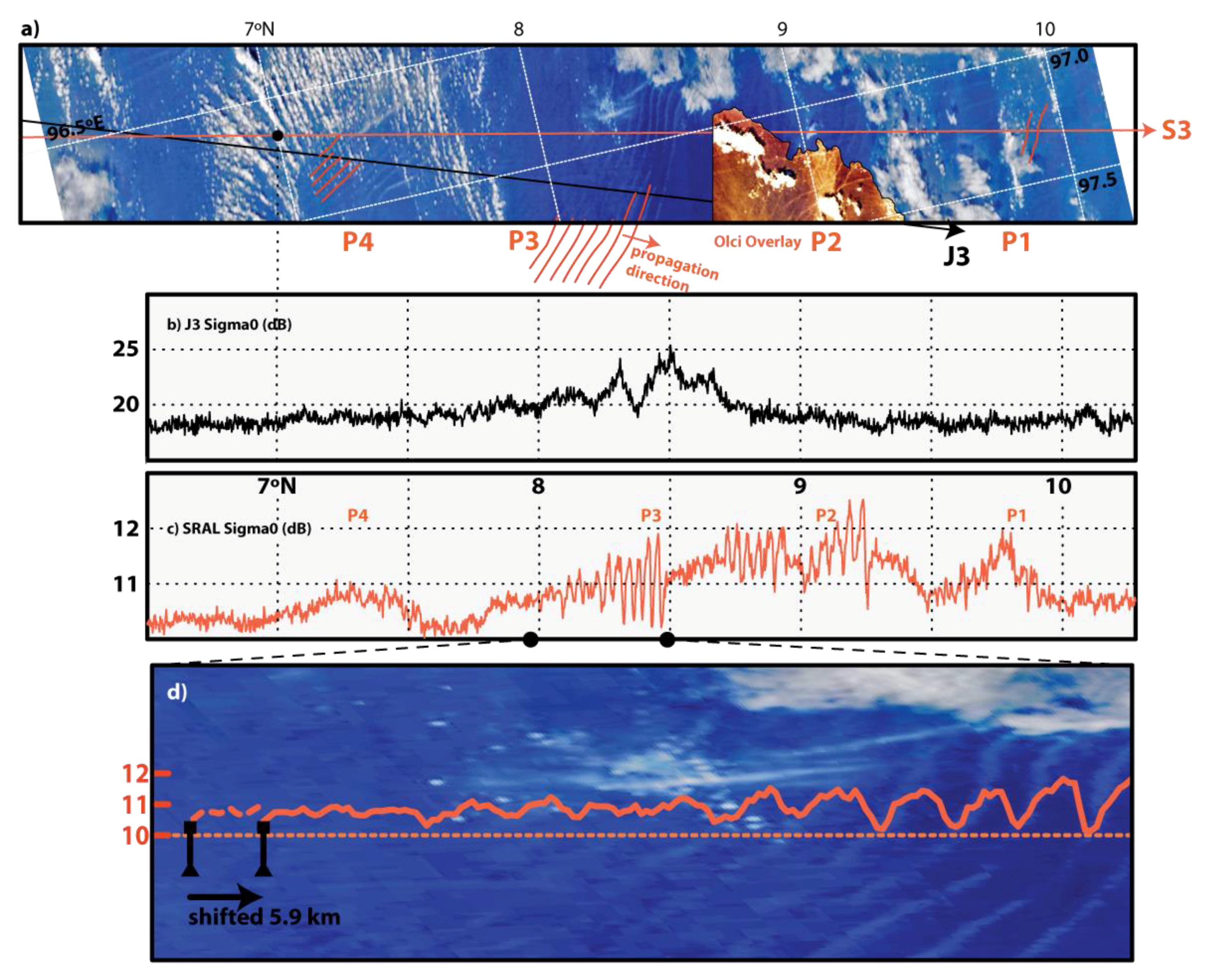
On 12 February 2017, Sentinel-3A overpassed the Andaman Sea (cycle 14; relative orbit number 175) at 03:37 UTC, near northern Sumatra and not far from where the earliest reports of ISWs in the Andaman Sea were made in the 1980s (see [3,20,21]). Large amplitude, long internal waves are observed in the corresponding OLCI image, as well as a Terra MODIS image acquired at 04:33 UTC (descending orbit). Since the OLCI image is partly contaminated by clouds, Figure 2a presents a composite that illustrates the 2D horizontal structure of the ISWs, which is visible in the OLCI and MODIS images together. For this particular case, a synergy is also possible with the Jason-3 high-rate (20 Hz) altimeter for which the along-track radar backscatter coefficient σ0 is displayed in Figure 2b in backscatter dB units (Ku-band). The corresponding SRAL along-track σ0 record is presented in Figure 2c. Note that backscatter oscillations in the SRAL, as much as 2 dB, are coincident with the ISWs crests and troughs. Four ISW packets, labelled P1 to P4, can be identified in the SRAL Ku-band along-track record, the most prominent being the packet labelled P3, which contains at least seven wave crests (propagating approximately along the direction indicated by the red arrow in Figure 2a). This packet, located between 8.0 and 8.5°N (Figure 2c) and whose wave crests are oriented approximately perpendicular to the satellite along-track direction, exhibits a rank-ordered amplitude character typical of ISWs [3], i.e., the leading wave in the wave train possesses the largest amplitude in the σ0 backscattered signal, as well as in the sunglint surface manifestations apparent in the visible imagery (MODIS). The bottom panel (Figure 2d) is a zoom in the Terra MODIS image, which is shifted south by 5.9 km to account for the time lapse between the SRAL and MODIS overpass of 56 min. Here we stress that the SRAL record is characterized by a decrease in backscatter (σ0) followed by an increase (of approximately the same strength) in the apparent direction of internal wave propagation, with respect to the background (unaffected by ISWs). On the contrary, the Jason-3 backscatter signature (Figure 2b) does not reveal the same fine structure of individual solitary waves. Moreover, it only captures one wave packet (that labelled P3 in Figure 2a,c) whose morphology does not provide as much detail as the SRAL, and whose signature is displaced north by some 0.2 degrees in relation to the SRAL. This displacement is due to the difference in overpass time, which is approximately 3.5 h between Jason-3 and MODIS. We further note that the wind speed retrieved from the SRAL was within 5–7 m/s (not shown), well within the range of pronounced contrasts in satellite visible imagery [22], while by the time of the Jason-3 overpass the wind speed had decreased.
3.2. Tropical Deep Atlantic Ocean off the Amazon River Mouth
The next example of ISW signatures in the SRAL selected for this paper is dated 11 October 2017 (cycle 23; relative orbit number 152) when the Sentinel-3A overflew the tropical Atlantic Ocean off the Amazon shelf break at 12:55 UTC. The region is a recently surveyed hotspot of intense ISWs that emanate from the steep shelf slopes off the Amazon River mouth into the open ocean, and whose wave crests extend for typically 200 km. Their surface manifestations are associated with intense wave breaking and roughness (see [23,24] and references therein; Kudryavtsev, pers. com.). Figure 3a displays a quasi-true color OLCI image of the region where the Sentinel-3A track (in red) intersects the ISW signatures (see dashed black circle in Figure 3a). The SRAL radargram (Ku-band waveforms in 20 Hz) displayed in Figure 3b is clearly sensitive to the ISW surface manifestations whose effects are seen around 4.25°N as a sharp discontinuity (or a dip) in the radar power levels. In more detail, Figure 3c shows average SRAL waveforms representative of the unperturbed background (blue curve) and the ground segment affected (i.e., perturbed) by the surface manifestations of ISWs (red curve). Note that the two (averaged) waveforms are similar in shape, but the perturbed curve has significantly attenuated backscatter power, particularly within the middle gates of the waveform.
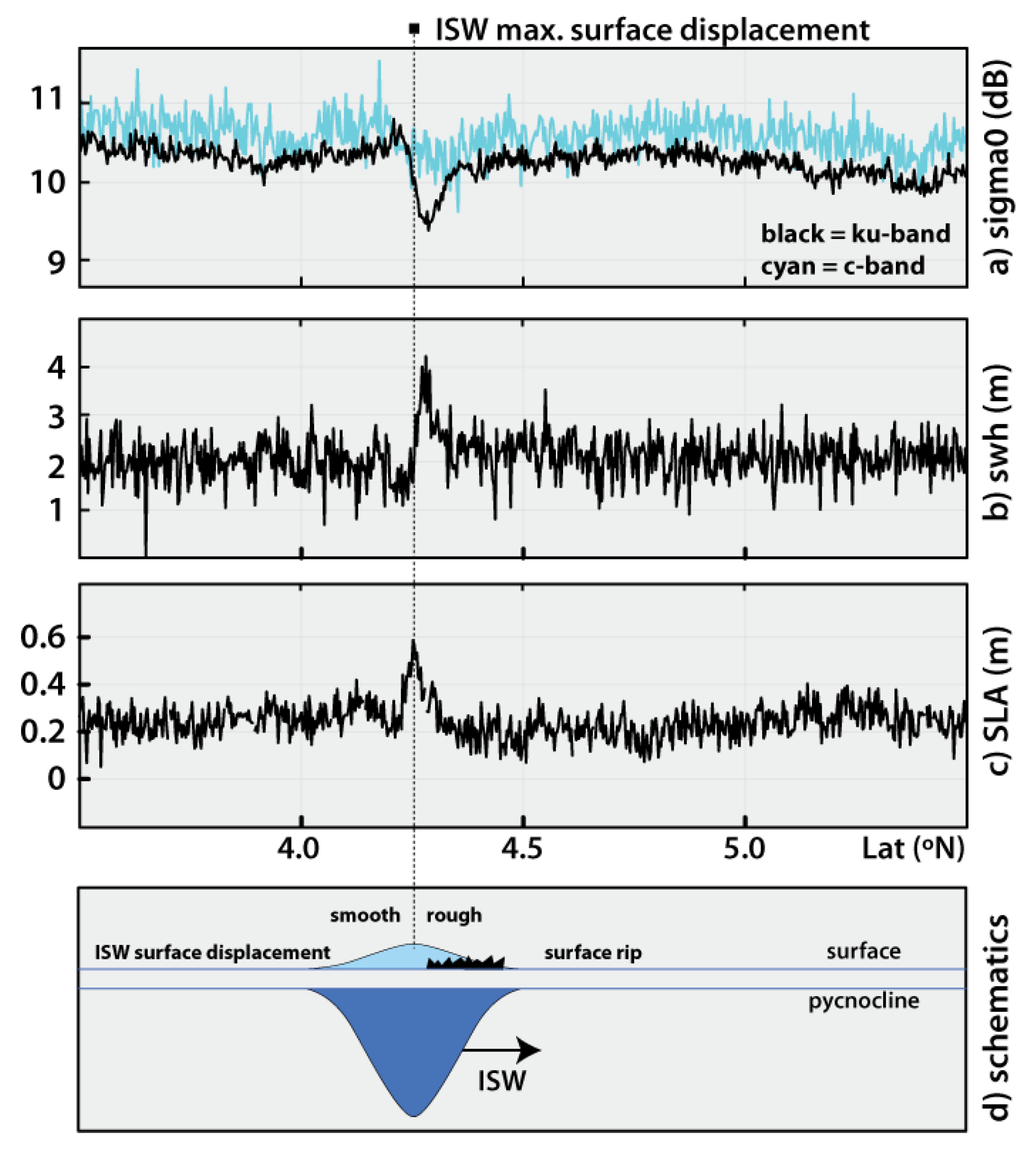
In order to characterize the ISW signatures in the SRAL retracked ocean geophysical parameters, Figure 4a shows the Ku-band and C-band backscatter variations across the solitary wave presented above (2017.10.11), i.e., in Figure 3a. In the Ku-band (dark curve in Figure 4a), there is a clear depression in σ0 (of almost 1 dB) near 4.3°N followed by (i.e., to the south) a slight backscatter increase (of only less than 0.5 dB) relative to the unperturbed background. The backscatter is much less affected by the ISWs at the C-band (see blue curve in Figure 4a). The wind speed retrieved from the SRAL is around 8 m/s (from the unperturbed surface ahead of the ISW), which is moderate and slightly higher than the previous example shown in Figure 2. Hence, this observation demonstrates that ISWs can be detected in this region in the SRAL, even at moderate wind speeds. There is also a signature of the ISW in SWH (Figure 4b) and in SLA (Figure 4c). It is clearly seen near 4.3°N with (positive) perturbations of as much as 2 m in SWH and as much as 40 cm in SLA. We emphasize the fact of the positive anomaly in SLA (40 cm upward), which is consistent with two-layer models of solitary wave theory (e.g., [3])—to be further discussed later. We also note in passing that a small shift exists between the maximum sigma0 and that of the SLA peak value. This shift is around 1500 m (or more) and, as illustrated in Figure 4d, it is likely a consequence of the nonlinearity of the waves (i.e., internal solitons of depression). Note that the SLA peak value is expected at the maximum downward displacement of the pycnocline (assuming a two-layer model), while the minimum in sigma0 occurs over the leading slope of the solitary wave where the surface roughness (and surface convergent rate) is maximum. Hence, for large solitary waves as those in Figure 3, a shift is expected between SLA peak and sigma0 minimum.
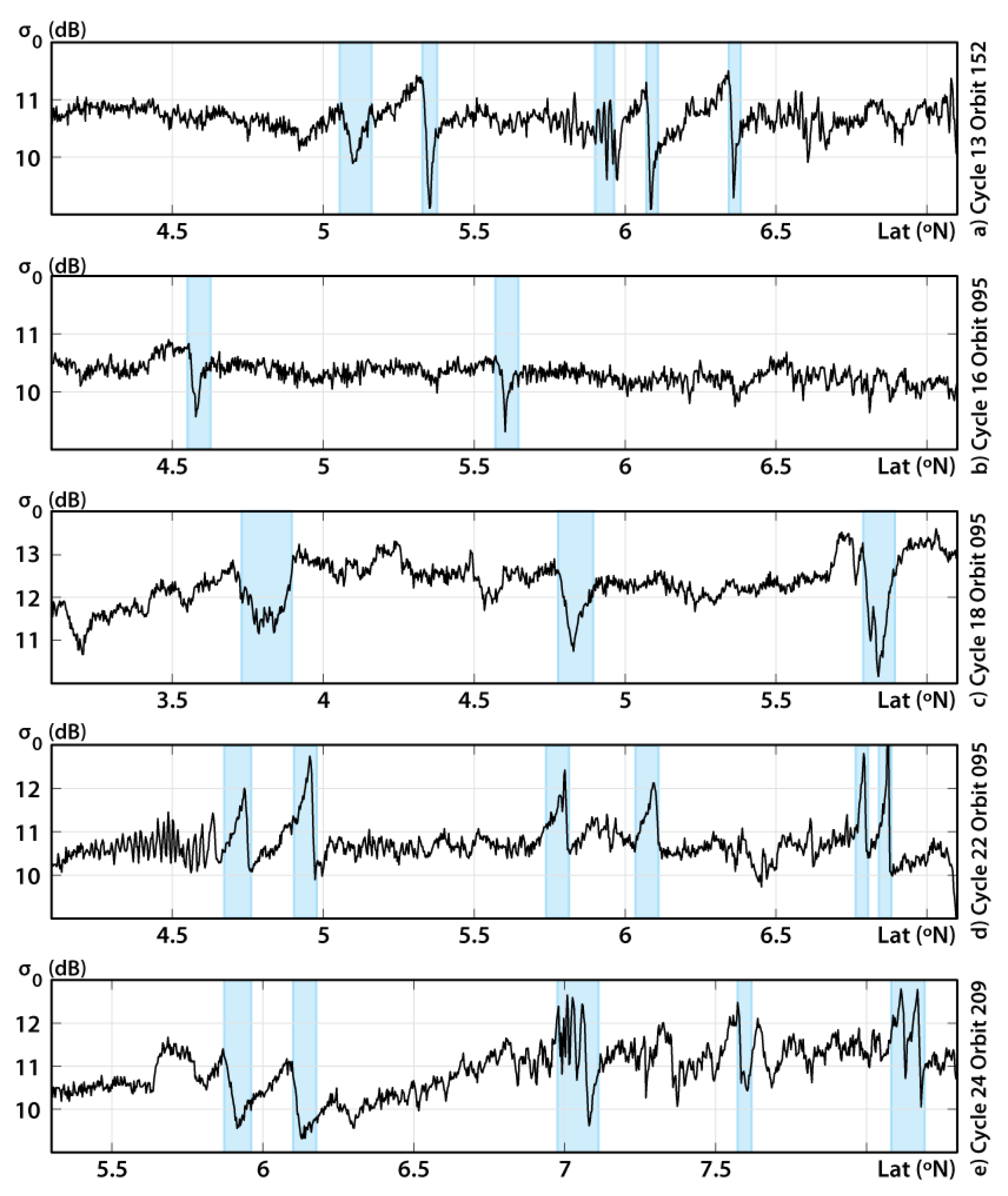
In what follows we describe the evidence of the presence of ISWs in a few more case studies, which are validated by inspection of the synergetic obtained with OLCI imagery (not shown). Table 1 lists along-track backscatter records of these case studies in the tropical Atlantic off the Amazon shelf. Since radar backscatter perturbations due to ISWs are more pronounced at the Ku-band, we show along-track records of radar backscatter (σ0) at the Ku-band in Figure 5. The region was selected based on our knowledge of the existence in the deep ocean of large amplitude ISWs [23] whose direction of propagation is at an angle of 15 to 30 degrees anti-clockwise from the satellite descending track. These ISWs propagate for distances exceeding 500 km offshore and possess strong imaging radar (SAR) signatures (see [23]). They are characterized by just a few solitons per wave train (typically 1–3) with typical scales of 5 km and, hence, are well within the SRAL along-track spatial resolution (see Figure 1c). The most evident signatures of solitary-like waves in the case studies presented in Figure 5 are hatched in light blue. We note that while most backscatter variations in Figure 5 exhibit positive and negative oscillations from a local mean background, in some cases mostly negative variations are observed (panel b and c) and in some others mostly positive variations are observed (panel d).
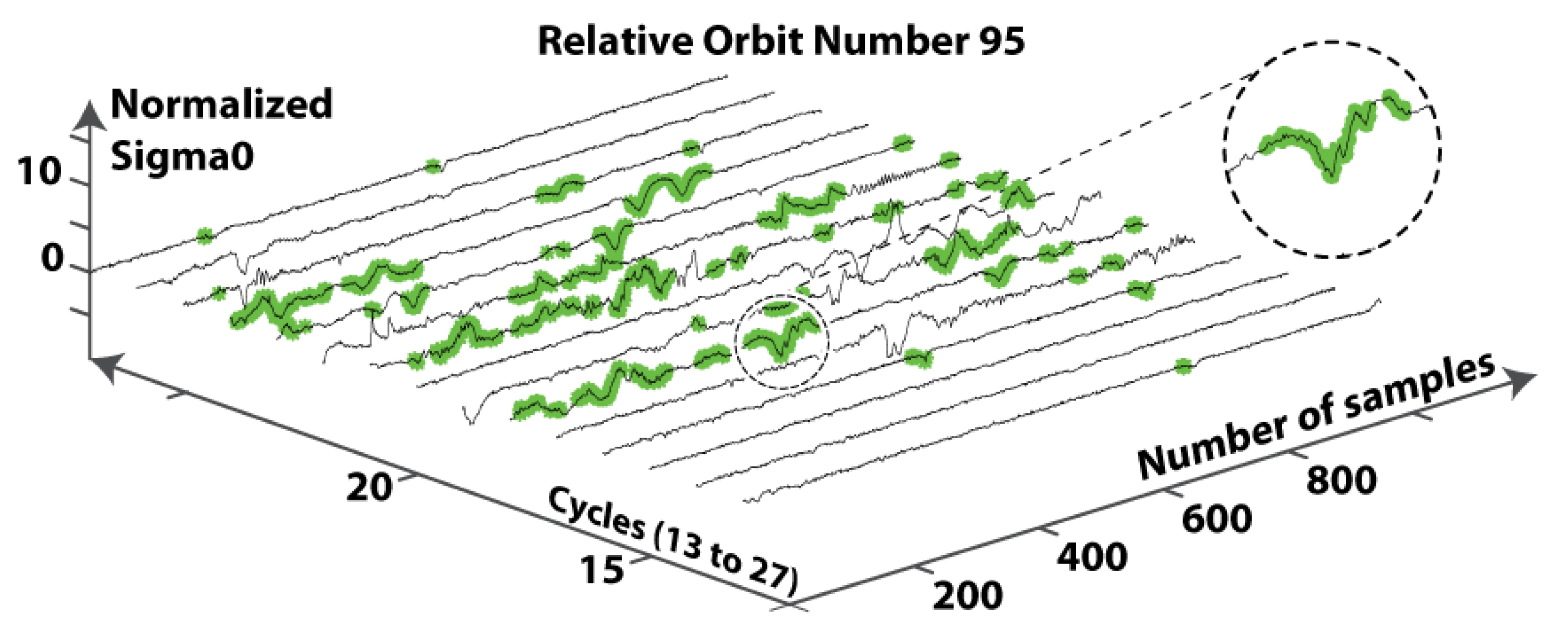
Figure 6 shows the results of the detection algorithm for the relative orbit number 95, cycles 13 through 27. Each record represents a stretch of approximately 300 km off the shelf break that would cross the ISW crests if the ISW events exist at the time of flyby. Note that 12 out of 15 cycles are detected as potentially affected by ISWs, which is in accord with previous findings presented by [23] who found that ISWs are quite frequent in the region and exist throughout the year and at any phase of the fortnightly tidal cycle. More than 80 ISW-like events are detected by the algorithm in the 15 cycles of the relative orbit 95.
4. Discussion
While MdS considered—for the pulse-limited Jason-2 radar altimeter—ISW-like events as only the observations of σ0 oscillations exceeding 2 dB from the surrounding background, and focused their attention on signals above 15 dB (i.e., sigma-naught blooms type of signatures), the SRAL offers enhanced signal-to-noise ratio (particularly for SLA), which results in a 40% lower noise level than the low rate mode (LRM) (see [11]). This feature of the SRAL indicates enhanced capabilities in the detection of surface manifestations of ISWs and allows us to relax MdS’s sigma-naught’s amplitude to less than 1 dB for the detection of ISWs. Furthermore, the SLA anomalies for Jason-2 reported in MdS, which are around −40 cm at a representative ISW wavelength, are systematically negative, i.e., the sea surface anomaly is measured as a dip of the sea surface level. This is certainly a nonphysical artifact of the MLE algorithms, which deal poorly with SLA for pulse-limited altimetry. The SLA produced by ISWs of depression (as most of them are in the deep ocean) should be positive according to theory, i.e., in opposite phase to the displacement of the pycnocline below (see e.g., [4]). This is what is observed with the new SRAL data where the ISW signatures are identified (see Table 1). The typical SLAs of +10 to +40 cm are reasonable and consistent with theoretical expectations.
In summary, a synergy approach between the SRAL and OLCI on board the Sentinel-3A has shown that the SAR mode altimetry can detect ISWs whose scales are less than 10 km. As the along-track footprints of SRAL are much finer than conventional pulse-limited altimeters, the trailing edges of the SRAL echoes are much less affected by ISWs than pulse-limited altimetry echoes whose power shifts toward trailing edges as a consequence of ISW inhomogeneities in the illuminated area. Because the SRAL waveforms are more robust and stable, it implies that the retracked geophysical parameters such as SLA and SWH from the internal wave field are more realistic compared with the unrealistic estimates from Jason-2 that are affected by the ISW-like events and significantly biased in scales of 10 km [14].
We now briefly discuss the character of the ISW SRAL backscatter oscillations in response to roughness variability induced by the surface manifestations of ISWs. While it is usually assumed that the SAR imaging mechanism of the ocean surface is dominated by Bragg (or resonant) scattering (i.e., for oblique viewing, typically 20° to 30° off-nadir), the altimeter observation geometry determines specular scattering as the major response mechanism (see e.g., [25]). Since the backscatter seen by the altimeter in space is restricted to a fraction of a degree around the nadir position, the scattering mechanism is essentially an optics-type reflection from thousands of specular points randomly distributed across the rough, moving sea surface [26]. This is quite different from the backscatter resulting from side-looking SAR images that is related to Bragg scattering. In a SAR image, a rougher surface appears brighter (positive variation from the local unperturbed mean backscatter) and a smoother (slick) surface appears darker (negative variation from the local mean backscatter). On the contrary, in the SRAL along-track altimeter records, radar backscatter from rougher sea surface patches appears attenuated in comparison to the unperturbed background, and the backscatter from a smooth sea surface patch appears enhanced in comparison to the unperturbed background. This is a reversed picture in comparison to imaging SARs [27] (see also Magalhaes and da Silva [14] and their Figure 2 comparing SAR imaging and conventional pulse-limited altimeter backscatter geometries).
The discussion above is relevant in the sense that surface manifestations of ISWs are characterized by enhanced and reduced roughness of the sea surface arrayed in parallel bands with scales of at least hundreds of meters wide and tens of kilometers long (see e.g., [27] and Figure 1). These bands result from the modulation of surface gravity-capillary waves due to convergent and divergent currents originated by the ISWs. For side-looking radar imaging, the theory developed in [27], based on weak hydrodynamic interaction theory and Bragg scattering theory, describes reasonably well the observed radar signatures of internal waves. When surface films are present in the water, the periodic convergence and divergence of the horizontal component of orbital velocity associated with the internal waves produces alternate bands of compaction and extension in the surface film that are sufficient to cause measurable differences in the rippling of the water by a slight breeze. In those instances, da Silva et al. [28] proposed that ISWs are imaged as dark bands on a gray radar background. On the contrary, when intense surface wave breaking is associated with ISWs (e.g., in deep water and tropical seas, such as the Andaman Sea and the tropical Atlantic off the Amazon shelf), ISW radar signatures are sometimes characterized by bright bands on a gray radar background (see e.g., [29]). Hence, ISW SAR signatures of an imaging radar exhibit essentially three possible morphology classes: positive and negative backscatter variations from a local unperturbed radar backscatter background [27] (see also Figure 1a,b); mostly positive variation from the local mean backscatter [23,29]; and mostly negative variation from the local mean backscatter [28,30]. The same kind of signature classification can be made for the SRAL based on observations such as those shown in Figure 5. In the SRAL, ISWs are expected to appear as reduced and increased backscatter from the radar unperturbed background when viewed from the upstream to the downstream propagation direction of ISWs. This is well seen in Figure 5a,e (cycles 13 and 24). In some cases, mostly enhanced backscatter variations from a mean background are observed, as in Figure 5d (cycle 22), which we interpret as a case when slicks are modulated by the ISWs. However, for the tropical Atlantic deep ocean region off the Amazon shelf, we frequently observe reduced backscatter compared to the mean background signal (Figure 5b,c; cycles 16 and 18; see also Figure 4a). We think this is evidence of intense small-scale roughness generated by meter-scale wave breaking, which is known to occur in this region ([24] and Kudryavtsev per. Comm.), and is expected due to surface wave–internal wave interaction. Finally, we reiterate that the morphology of the backscatter variations are reversed between SAR imaging devices and the SRAL (i.e., enhanced/reduced versus reduced/ enhanced, respectively, in the direction of propagation), which has been quite helpful in interpreting ISW altimeter records such as those shown in Figure 5a,e.
Scrutiny of the case studies discussed in this paper (Table 1 and Figure 2, Figure 4, and Figure 5) reveals that the impacts of ISWs on SRAL altimetry data are more significant under low wind conditions (e.g., 4 m/s) than under moderate wind conditions. In fact, the Jason-3 observation shown in Figure 2b of the same wave packet viewed by the SRAL (Figure 2c) is in the form of a σ0 bloom, a term used for excessively high radar returns [31,32]. It is therefore important to recognize that ISW packets may be another factor causing σ0 blooms in radar altimetry data. Cheng et al. 2017 [32] reported a similar phenomenon in the case of oil slicks on the sea surface, i.e., that with an increase in wind speed, the impact of oil on σ0 decreases for both Ku- and C-bands of Jason-2. In the case of short-period internal waves such as the ISWs analyzed in this paper, straining effects due to internal waves on short capillary-gravity waves have a greater impact at lower wind speeds, which is in accord with the hydrodynamic modulation theory. This theory, also known as the relaxation model or relaxation time approximation, predicts that at moderate to high wind speeds, relaxation rates (inverse of relaxation times) are smaller than at low wind speeds. The relaxation time is the time duration over which waves of wavenumber k remain strained until they reach equilibrium with the wave spectrum under the influence of wind forcing and dissipation processes. This implies that as the wind speed increases, the radar contrasts are expected to become weaker. The hydrodynamic modulation theory is generally assumed as a first-order approach to describe radar contrasts of internal waves in SAR images [27]. The same is true when film slicks contribute to the surface manifestations of ISWs [28,30,33], and hence the findings reported by Cheng et al. (2017) [32] are consistent with the observations in this paper. We finally note that the same wind effects on ISW radar contrasts are reported in [28] for ERS-1/2 SAR images obtained at C-band.
5. Conclusions
In summary, the synergy between Sentinel’s-3A SRAL and OLCI has shown that altimeters operating in SAR mode are capable of detecting the presence of ISWs as backscatter variations along track when the satellite track traverses the ISW’s surface manifestations (parallel bands along crests and troughs) in an oblique direction. The radar cross-section perturbations are accompanied by positive SLAs and SWHs (Table 1). The SRAL echoes become significantly perturbed in the presence of ISWs, which can be identified in the radargram waveforms. As the along-track sharpened SRAL footprints cross ISWs, current Level-2 ocean product waveforms change significantly at scales of less than 10 km (Figure 3b,c). Similar results have been discussed in [14] for conventional pulse-limited altimeters (i.e., Jason-2) as a consequence of ISW inhomogeneities within the much larger footprint area. In the case of conventional pulse-limited altimeters, such as Jason-2/3, the ISW roughness changes within a footprint, meaning that the assumption of a uniform (Brown) surface is in essence invalid, rendering essentially unrealistic retracked parameters. This problem seems less severe for the SRAL, as SLAs are within the expected values for ISWs of pycnocline depression (as those observed). An automated method for ISW detection in the SRAL has been developed and applied to the tropical Atlantic Ocean off the Amazon shelf (a stretch of more than 300 km, approximately from 4°N to 8°N). The method includes rain flagging based on liquid water content and water vapor estimated from the microwave radiometer, high frequency feature detection based on wavelet analysis of radar backscatter and coincident positive SLAs. The results are illustrated in Figure 6, which comprises the detection of more than 80 events in 12 out of 15 cycles from relative orbit 095. The detected rate is in accord with our expectations and knowledge of ISWs in the study region [23].
A major prospect is then that ISWs could be routinely detected in SAR mode altimetry data (Sentinel-3A and 3B) once more robust detection algorithms are developed and properly validated. Validation would require a test site with simultaneous measurements of ISWs and SRAL overpasses. This would require a joint effort between independent research projects and funding, which is not within the scope of our investigation at present. Instead, we rely on our knowledge of detection of ISWs in OLCI and MODIS to validate the ISW observations with the SRAL. The SRAL offers some improvements in relation to conventional pulse-limited altimeters (e.g., Jason-2/3), such as better along-track resolution and lower noise level, which is particularly important for SLA realistic estimates. The typical SLAs of +10 to +40 cm are reasonable and consistent with theoretical expectations of two-layer internal wave models, and here all ISW-like events satisfy the condition that SLA variance exceeds 6 cm at the ISW scales. These improved SLA estimates at short-scales are an important feature of the SRAL, which can be used in future studies to optimize ISW detection algorithms. ISW-like signals can be distinguished from other oceanic and atmospheric high-frequency phenomena when those other phenomena do not provoke an SLA. Such would be the case, for example, with natural organic films or (sufficiently thin) oil spills that may not generate an SLA because they may lack a 3D baroclinic dynamic nature. Finally, we note that a forthcoming paper addressing the full analysis of SAR signatures of ISWs with the Sentinel-3 SRAL measurements over oceans and its detection algorithm based on wavelet analysis will complete the present report, which is focused on documenting our preliminary results.
Acknowledgments
The authors would like to thank the European Space Agency (ESA) and all Sentinel-3 Data Production Teams. This work was supported in part by FCT under Grant SFRH/BPD/84420/2012, and in part by Project Radar Altimeter Detection of Internal Solitary Waves in the Ocean as part of the Ocean Surface Topography Science Team in the frame of the CNES/EUMETSAT Research Announcement under Grant CNES-DIA/TEC-2016.8595 and Grant EUM/LEO-JAS3/DOC/16/852054. We thank three anonymous reviewers whose comments contributed to improve the quality of this paper.
Author Contributions
A.M.S-F. conceived and designed the wavelet algorithm to detect internal waves and processed all the satellite data; A.M.S-F. and J.C.B.d.S. analyzed the data; J.M.M. contributed with computer code to process the original Level-2 SRAL and Jason-3 data; J.C.B.d.S. wrote the paper and the other authors edited it. All authors were involved in figure preparation.
Conflicts of Interest
The authors declare no conflict of interest.
References
- Eckart, C. Internal Waves in the Ocean. Phys. Fluids (1958–1988) 1961, 4, 791–799. [Google Scholar] [CrossRef]
- Kunze, E. Internal-Wave-Driven Mixing: Global Geography and Budgets. J. Phys. Oceanogr. 2017, 47, 1325–1345. [Google Scholar] [CrossRef]
- Osborne, A.R.; Burch, T.L. Internal Solitons in the Andaman Sea. Sci. New Ser. 1980, 208, 451–460. [Google Scholar] [CrossRef] [PubMed]
- Gill, A.E. Atmosphere-Ocean Dynamics; International Geophysics Series; Donn, W.L., Ed.; Academic Press: San Diego, CA, USA, 1982; Volume 30, p. 662. [Google Scholar]
- Hughes, B.A.; Grant, H.L. The Effect of Internal Waves on Surface Wind Waves, 1. Experimental Measurements. J. Geophys. Res. 1978, 83, 443–454. [Google Scholar] [CrossRef]
- Frew, N.M.; Glover, D.M.; Bock, E.J.; McCue, S.J. A new approach to estimation of global air-sea gas transfer velocity fields using dual-frequency altimeter backscatter. J. Geophys. Res. 2007, 112, C11003. [Google Scholar] [CrossRef]
- Kudryavtsev, V.; Myasoedov, A.; Chapron, B.; Johannessen, J.A.; Collard, F. Joint sun-gitter and radar imagery of surface slicks. Remote Sens. Environ. 2012, 120, 123–132. [Google Scholar] [CrossRef]
- ESA. Sentinel-1 Observation Scenario. Available online: https://sentinel.esa.int/web/sentinel/missions/sentinel-1/observation-scenario (accessed on 26 March 2018).
- Raney, R.K. The Delay/Doppler Radar Altimeter. IEEE Trans. Geosci. Remote Sens. 1998, 36, 1578–1588. [Google Scholar] [CrossRef]
- Donlon, C.; Berruti, B.; Buongiorno, A.; Ferreira, M.-H.; Féménias, P.; Frerick, J.; Goryl, P.; Klein, U.; Laur, H.; Mavrocordatos, C.; et al. The Global Monitoring for Environment and Security (GMES) Sentinel-3 mission. Remote Sens. Environ. 2012, 120, 37–57. [Google Scholar] [CrossRef]
- Boy, F.; Desjonquères, J.D.; Picot, N.; Moreau, T.; Raynal, M. CryoSat-2 SAR-Mode Over Oceans: Processing Methods, Global Assessment, and Benefits. IEEE Trans. Geosci. Remote Sens. 2017, 55, 148–158. [Google Scholar] [CrossRef]
- Thibaut, P.; Poisson, J.C.; Bronner, E.; Picot, N. Relative performance of the MLE3 and MLE4 retracking algorithms on Jason-2 altimeter waveforms. Mar. Geod. 2010, 33, 317–335. [Google Scholar] [CrossRef]
- Ray, R.D.; Mitchum, G.T. Surface manifestation of internal tides generated near Hawaii. Geophys. Res. Lett. 1996, 23, 2101–2104. [Google Scholar] [CrossRef]
- Magalhaes, J.M.; da Silva, J.C.B. Satellite Altimetry Observations of Large-Scale Internal Solitary Waves. IEEE Geosci. Remote Sens. Lett. 2017, 14, 534–538. [Google Scholar] [CrossRef]
- Brown, G.S. The average impulse response of a rough surface and its applications. IEEE Trans. Antennas Propag. 1977, 25, 67–74. [Google Scholar] [CrossRef]
- Tournadre, J.; Morland, J.C. The Effects of Rain on TOPEX/Poseidon Altimeter data. IEEE Trans. Geosci. Remote Sens. 1997, 35, 1117–1135. [Google Scholar] [CrossRef]
- Da Silva, J.C.B.; Cerqueira, A.L.F. A note on radar altimeter signatures of Internal Solitary Waves in the ocean. In Proceedings of the Remote Sensing of the Ocean, Sea Ice, Coastal Waters, and Large Water Regions, Edinburgh, Scotland, UK, 26–27 September 2016; Bostater, C.R., Neyt, X., Nichol, C., Aldred, O., Eds.; SPIE: Bellingham, WA, USA, 2016; Volume 9999, p. 14. [Google Scholar]
- Tournadre, J.; Lambin-Artru, J.; Steunou, N. Could and Rain Effects on Altika/SARAL Ka-Band Radar Altimeter-Part II: Definition of a Rain/Cloud Flag. IEEE Trans. Geosci. Remote Sens. 2009, 47, 1818–1826. [Google Scholar] [CrossRef]
- Ródenas, J.A.; Garello, R. Wavelet Analysis in SAR Ocean Image Profiles for Internal Wave Detection and Wavelength Estimation. IEEE Trans. Geosci. Remote Sens. 1997, 35, 933–945. [Google Scholar] [CrossRef]
- Maury, M.F. The Physical Geography of the Sea and Its Meteorology; Harper: New York, NY, USA, 1861; p. 457. [Google Scholar]
- Perry, R.B.; Schimke, G.R. Large-Amplitude Internal Waves Observed off the Northwest Coast of Sumatra. J. Geophys. Res. 1965, 70, 2319–2324. [Google Scholar] [CrossRef]
- Jackson, C.R.; Alpers, W. The role of the critical angle in brightness reversals on sunglint images of the sea surface. J. Geophys. Res. 2010, 115, C09019. [Google Scholar] [CrossRef]
- Magalhaes, J.M.; da Silva, J.C.B.; Buijsman, M.C.; Garcia, C.A.E. Effect of the North Equatorial Counter Current on the generation and propagation of internal solitary waves off the Amazon shelf (SAR observations). Ocean Sci. 2016, 12, 243–255. [Google Scholar] [CrossRef]
- Kuznetsov, A.S.; Paramonov, A.N.; Stepanyants, Y.A. Investigation of solitary internal waves in the tropic zone of West Atlantic. Izv. Atmos. Ocean. Phys. 1984, 20, 975–984. (In Russian) [Google Scholar]
- Valenzuela, G.R. Theories for the interaction of electromagnetic and oceanic waves: A Review. Bound. Layer Meteorol. 1978, 13, 61–85. [Google Scholar] [CrossRef]
- Barrick, D.E.; Lipa, B.J. Analysis and Interpretation of Altimeter Sea Echo. In Satellite Oceanic Remote Sensing; Advances in Geophysics Series; Saltzman, B., Ed.; Academic Press: Orlando, FL, USA, 1985; Volume 27, pp. 61–100. ISBN 0-12-018827-9. [Google Scholar]
- Alpers, W. Theory of radar imaging of internal waves. Nature 1985, 314, 245–247. [Google Scholar] [CrossRef]
- Da Silva, J.C.B.; Ermakov, S.A.; Robinson, I.S.; Jeans, D.R.G.; Kijashko, S.V. Role of surface films in ERS SAR signatures of internal waves on the shelf—1. Short-period internal waves. J. Geophys. Res. 1998, 103, 8009–8031. [Google Scholar] [CrossRef]
- Kudryavtsev, V.; Akimov, D.; Johannessen, J.A.; Chapron, B. On radar imaging of current features: 1. Model and comparison with observations. J. Geophys. Res. 2005, 110, C007016. [Google Scholar] [CrossRef]
- Da Silva, J.C.B.; Ermakov, S.A.; Robinson, I.S. Role of surface films in ERS SAR signatures of internal waves on the shelf—3. Mode transitions. J. Geophys. Res. 2000, 105, 24089–24104. [Google Scholar] [CrossRef]
- Mitchum, G.; Hancock, D.; Hayne, G.; Vandemark, D. Blooms of σ0 in the TOPEX radar altimeter data. J. Atmos. Ocean. Technol. 2004, 21, 1232–1245. [Google Scholar] [CrossRef]
- Cheng, Y.; Tournadre, J.; Li, X.; Xu, Q.; Chapron, B. Impacts of oil spills on altimeter waveforms and radar backscatter cross section. J. Geophys. Res. Oceans 2017, 122, 3621–3637. [Google Scholar] [CrossRef]
- Ermakov, S.A.; Salashin, S.; Panchenko, A. Film slicks on the sea surface and some mechanisms of their formation. Dyn. Atmos. Oceans 1992, 16, 279–304. [Google Scholar] [CrossRef]
Figure 1.
(a) Subset of an Envisat-ASAR (Advanced Synthetic Aperture Radar) image acquired in image precision mode dated 10 May 2005 at 03:29 UTC. The image shows a typical internal solitary wave (ISW) packet propagating northeast in the Andaman Sea (see inset in top-right corner for location). (b) ISW relative intensity retrieved from the black rectangle in the panel (a). (c) Schematic representation of ISW sea surface roughness patterns alongside typical altimetry footprints for Jason-2 and the synthetic aperture radar altimeter (SRAL). See text for more details.

Figure 2.
(a) Composite map of Sentinel-3A Ocean Land Colour Imager (OLCI) (partially shown in orange tones) with wave crests delineated as orange curves on top of a Terra Moderate Resolution Imaging Spectroradiometer (MODIS) acquisition (blue tones). The Sentinel-3A satellite track projected on the ground is marked with a red line while longitudes and latitudes are marked in white. The Jason-3 ground track is also shown in a black line. (b) Jason-3 along-track radar backscatter record for the Ku-band (20 Hz) in (dB) units (σ0). (c) Along-track SRAL record in backscatter (dB) units (σ0) for the Ku-band. The labels P1 to P4 indicate different ISW trains and latitudes are displayed on the top of the vertical grid. (d) Enlargement of image section in the latitude interval [8.0, 8.5]°N showing the surface manifestations of ISWs due to sunglint co-located with the SRAL backscatter record. Note that the backscatter record was displaced by 5.9 km to account for the internal wave propagation between the times of MODIS and Sentinel-3A acquisitions (see text for details).

Figure 3.
(a) Sentinel-3A OLCI image (Level 1b) dated 2017.10.11 acquired at 12:54:29 UTC (start time) presented in quasi-true color. The red line represents the Sentinel-3A track on the ground. (b) Radargram of SRAL composed of a sequence of 20 Hz waveforms. Backscatter power is represented in color with arbitrary units displayed in the color bar. (c) Averaged waveforms for perturbed (red) and unperturbed (blue) sea surface conditions.

Figure 4.
(a) Along-track backscatter (σ0) for Ku-band (black) and C-band (light blue). (b) Along-track SRAL record of SWH (significant wave height) showing a pronounced increase of retrieved SWH at approximately 4.3°N, from the average 2 m to 4 m. (c) Sea level anomaly (SLA) in SAR mode for the same ground segment where a sea surface elevation anomaly of approximately 0.4 m can be seen at the same location of the ISW signature. (d) Schematic representation of an interfacial ISW of depression showing a maximum of the surface water displacement over its trough, in between its rough and smooth surface manifestations. See text for more details.

Figure 5.
Selection of Sentinel-3A SRAL observations (Ku-band) over the tropical Atlantic Ocean off the Amazon shelf where signatures of surface manifestations of ISWs can be identified (in light blue rectangles, see also Table 1 for details).
Figure 5.
Selection of Sentinel-3A SRAL observations (Ku-band) over the tropical Atlantic Ocean off the Amazon shelf where signatures of surface manifestations of ISWs can be identified (in light blue rectangles, see also Table 1 for details).

Figure 6.
Graphic representation of a sequence of 15 cycles for relative orbit number 95 of Sentinel-3A (SRAL sigma0) for a stretch over more than 300 km off the Amazon shelf in the tropical Atlantic Ocean. The green segments indicate detection of ISWs by the algorithm developed in this paper.
Figure 6.
Graphic representation of a sequence of 15 cycles for relative orbit number 95 of Sentinel-3A (SRAL sigma0) for a stretch over more than 300 km off the Amazon shelf in the tropical Atlantic Ocean. The green segments indicate detection of ISWs by the algorithm developed in this paper.


Table 1.
A summary of selected synthetic aperture radar altimeter (SRAL) observations of internal solitary waves (ISWs) off the Amazon shelf confirmed in Ocean Land Colour Imager (OLCI) images, with corresponding geophysical parameter variations and wind velocities at the time of acquisition. ΔσKu refers to peak-to-trough variations of sigma0 for a single event; ΔSLA is peak-to-trough variation of the sea level anomaly signal for a single event; ΔSWH is peak-to-trough variation of the significant wave height signal for a single event.
| Cycle | Rel. Orbit | Date | |ΔσKu| (dB) | ΔSLA (cm) | ΔSWH (m) | Wind Speed (m/s) |
|---|---|---|---|---|---|---|
| 013 | 152 | 2017.01.14 | 2.3 | 33 | 1.6 | 7 |
| 016 | 095 | 2017.04.01 | 1.3 | 25 | 2.0 | 8 |
| 018 | 095 | 2017.05.25 | 3.3 | 48 | 2.1 | 4 |
| 022 | 095 | 2017.09.10 | 1.9 | 24 | 1.6 | 7 |
| 024 | 209 | 2017.11.11 | 2.8 | 12 | 2.7 | 5 |
© 2018 by the authors. Licensee MDPI, Basel, Switzerland. This article is an open access article distributed under the terms and conditions of the Creative Commons Attribution (CC BY) license (http://creativecommons.org/licenses/by/4.0/).
Share and Cite
MDPI and ACS Style
Santos-Ferreira, A.M.; Da Silva, J.C.B.; Magalhaes, J.M. SAR Mode Altimetry Observations of Internal Solitary Waves in the Tropical Ocean Part 1: Case Studies. Remote Sens. 2018, 10, 644. https://doi.org/10.3390/rs10040644
AMA Style
Santos-Ferreira AM, Da Silva JCB, Magalhaes JM. SAR Mode Altimetry Observations of Internal Solitary Waves in the Tropical Ocean Part 1: Case Studies. Remote Sensing. 2018; 10(4):644. https://doi.org/10.3390/rs10040644
Chicago/Turabian StyleSantos-Ferreira, Adriana M., José C. B. Da Silva, and Jorge M. Magalhaes. 2018. "SAR Mode Altimetry Observations of Internal Solitary Waves in the Tropical Ocean Part 1: Case Studies" Remote Sensing 10, no. 4: 644. https://doi.org/10.3390/rs10040644
Note that from the first issue of 2016, this journal uses article numbers instead of page numbers. See further details here.