Enhanced Modeling of Annual Temperature Cycles with Temporally Discrete Remotely Sensed Thermal Observations

Abstract
:
1. Introduction
2. Materials and Methods
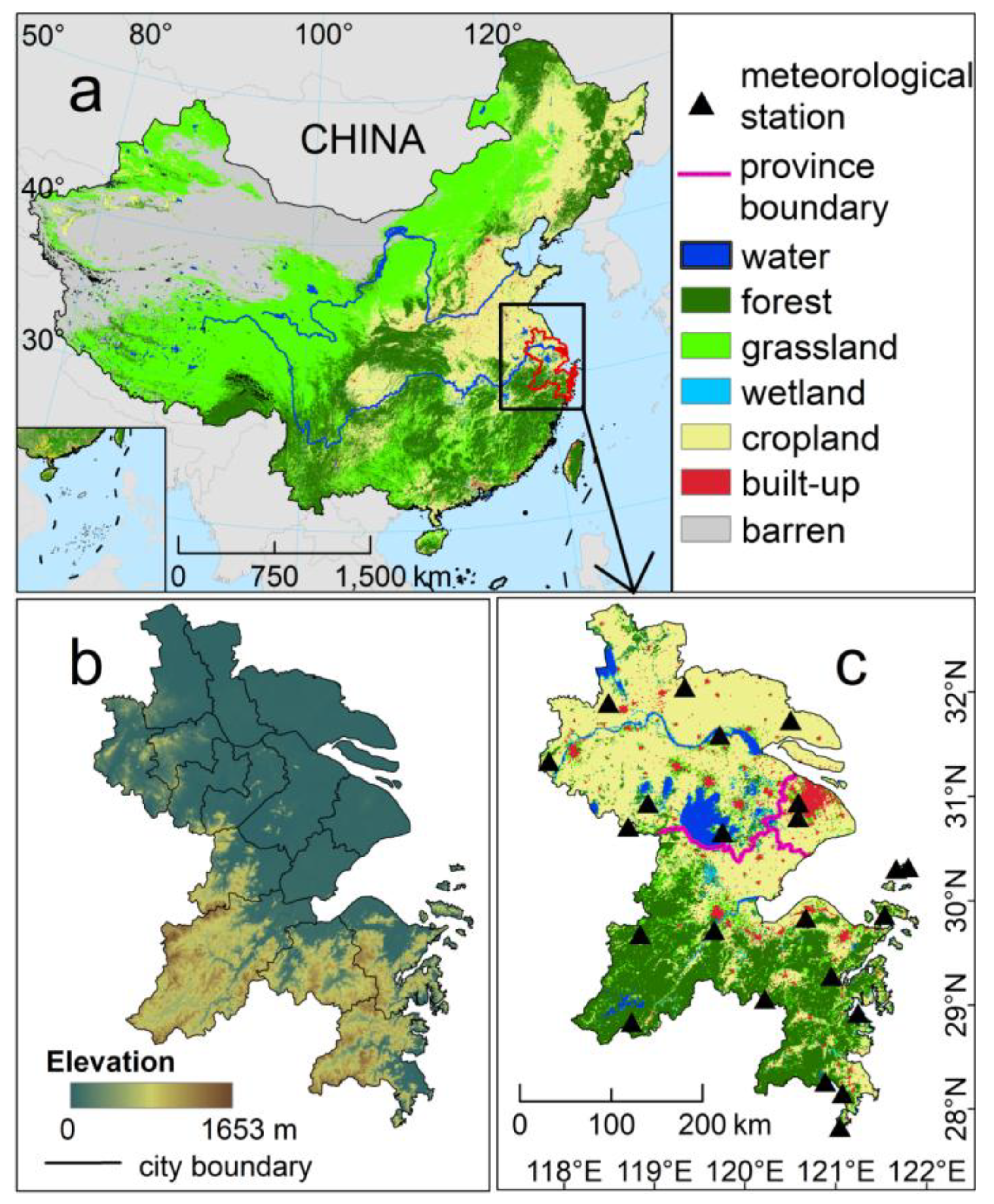
2.1. Study Area and Data
2.2. Method
2.2.1. Standard ATC Model
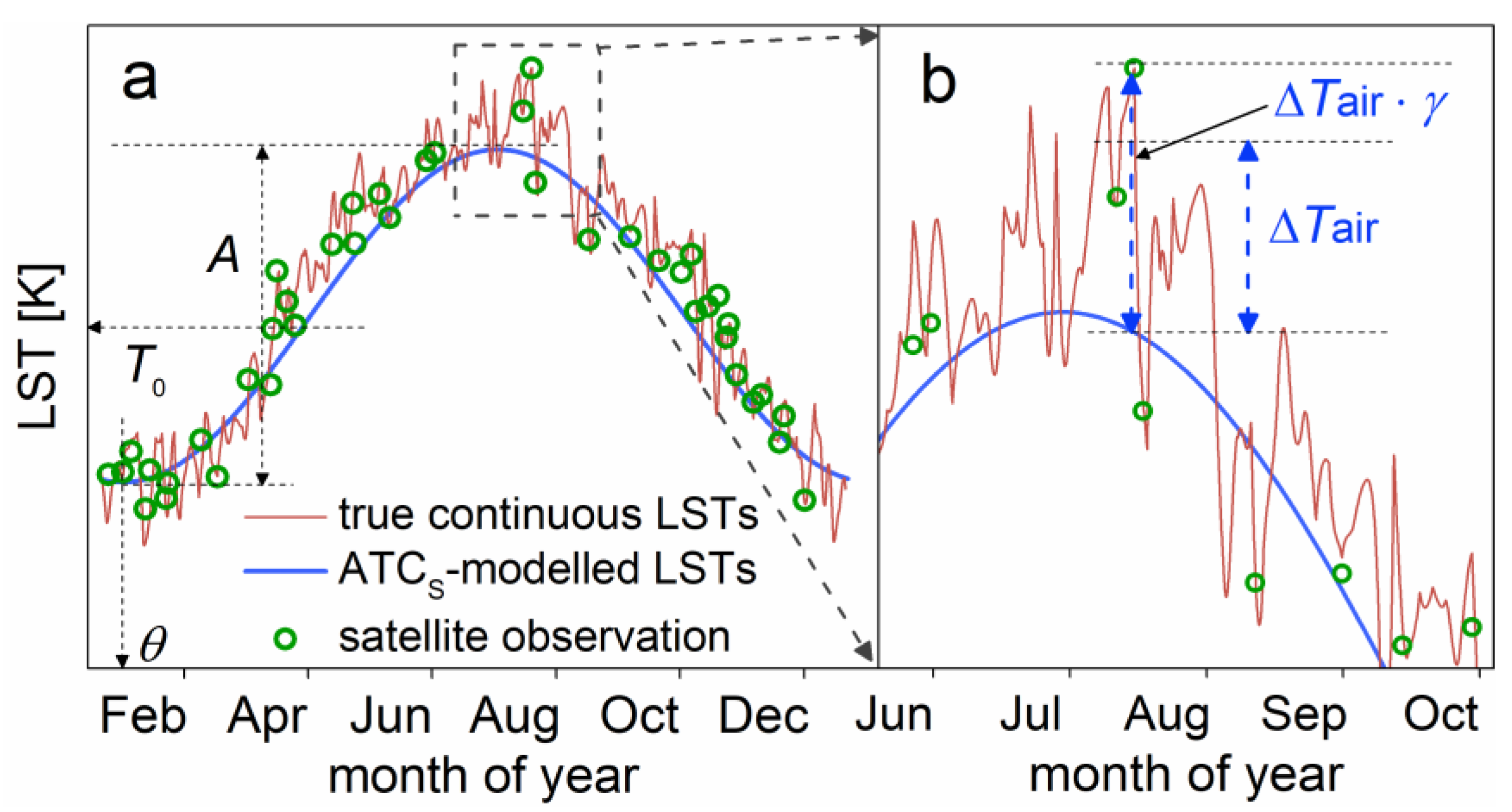
2.2.2. Enhanced ATC Model
2.2.3. Solution of the Forward ATCE and Validation Schemes
3. Results and Discussion
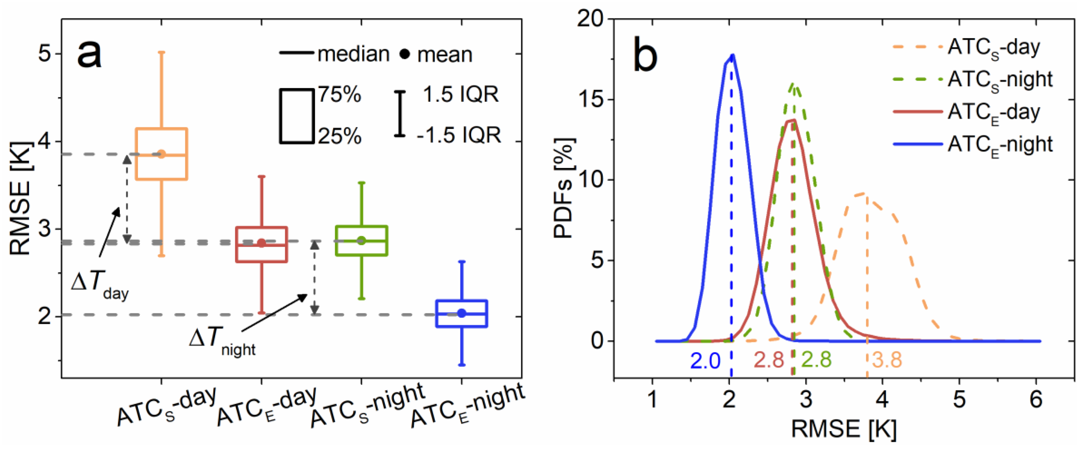
3.1. Overall and Spatial Patterns of Model Performances
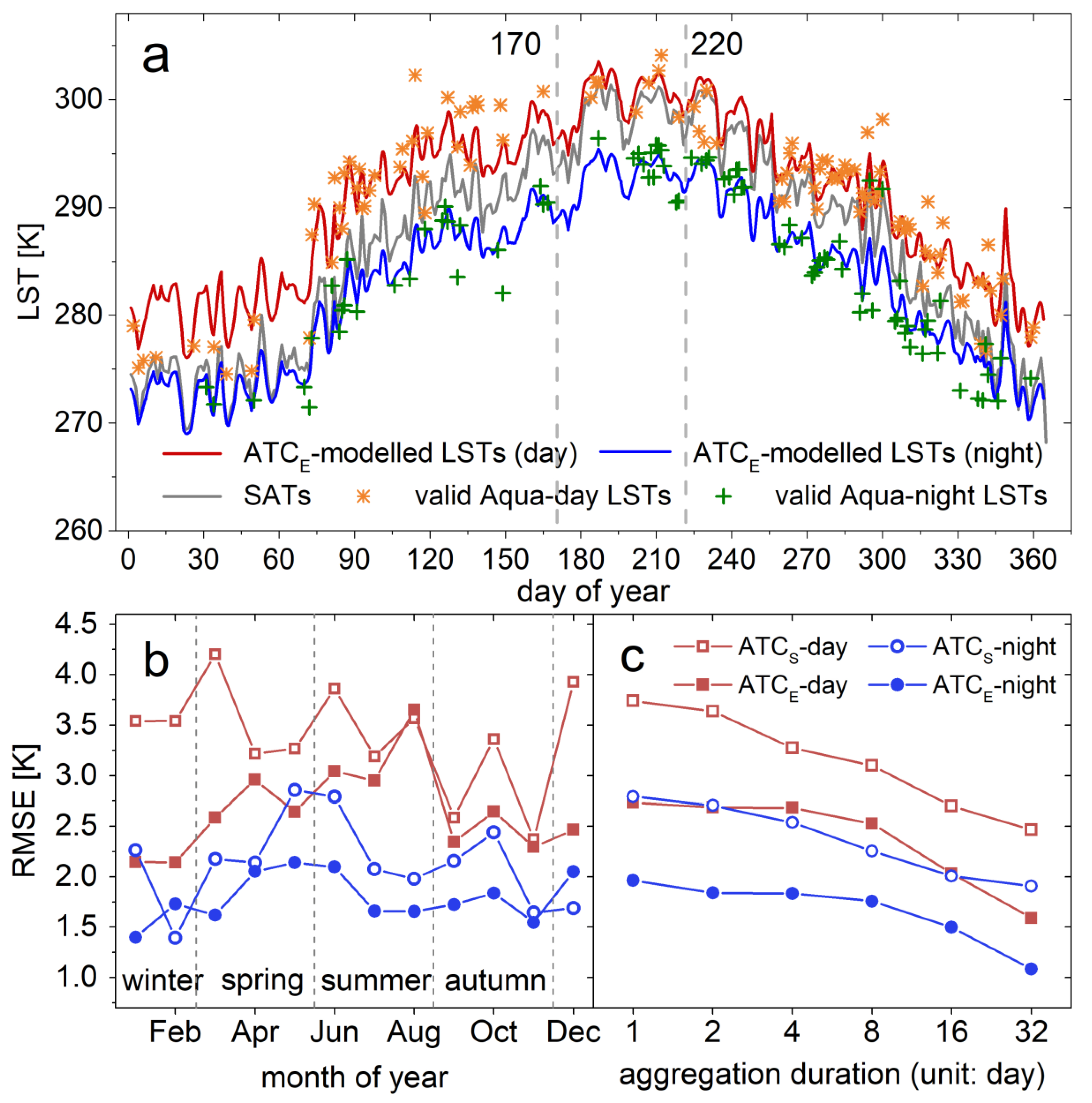
3.2. Temporal Patterns of Model Performances
3.3. Prospects and Limitations
4. Conclusions
Acknowledgments
Author Contributions
Conflicts of Interest
References
- Li, Z.; Tang, B.; Wu, H.; Ren, H.; Yan, G.; Wan, Z.; Trigo, I.F.; Sobrino, J.A. Satellite-derived land surface temperature: Current status and perspectives. Remote Sens. Environ. 2013, 131, 14–37. [Google Scholar] [CrossRef]
- Cammalleri, C.; Anderson, M.C.; Gao, F.; Hain, C.R.; Kustas, W.P. Mapping daily evapotranspiration at field scales over rainfed and irrigated agricultural areas using remote sensing data fusion. Agric. For. Meteorol. 2014, 186, 1–11. [Google Scholar] [CrossRef]
- Voogt, J.A.; Oke, T.R. Thermal remote sensing of urban climates. Remote Sens. Environ. 2003, 86, 370–384. [Google Scholar] [CrossRef]
- Giglio, L.; Descloitres, J.; Justice, C.O.; Kaufman, Y.J. An enhanced contextual fire detection algorithm for MODIS. Remote Sens. Environ. 2003, 87, 273–282. [Google Scholar] [CrossRef]
- Ramsey, M.S.; Harris, A.J.L. Volcanology 2020: How will thermal remote sensing of volcanic surface activity evolve over the next decade. J. Volcanol. Geotherm. Res. 2013, 249, 217–233. [Google Scholar] [CrossRef]
- Qin, K.; Wu, L.; De, S.A.; Gianfranco, C. Preliminary analysis of surface temperature anomalies that preceded the two major Emilia 2012 earthquakes (Italy). Ann. Geophys. 2012, 55, 823–828. [Google Scholar]
- Zhan, W.; Zhou, J.; Ju, W.; Li, M.; Sandholt, I.; Voogt, J.; Yu, C. Remotely sensed soil temperatures beneath snow-free skin-surface using thermal observations from tandem polar-orbiting satellites: An analytical three-time-scale model. Remote Sens. Environ. 2014, 143, 1–14. [Google Scholar] [CrossRef]
- Quan, J.; Zhan, W.; Chen, Y.; Wang, M.; Wang, J. Time series decomposition of remotely sensed land surface temperature and investigation of trends and seasonal variations in surface urban heat islands. J. Geophys. Res. Atmos. 2016, 121, 2638–2657. [Google Scholar] [CrossRef]
- Fu, P.; Weng, Q. Consistent land surface temperature data generation from irregularly spaced Landsat imagery. Remote Sens. Environ. 2016, 184, 175–187. [Google Scholar] [CrossRef]
- Sobrino, J.A.; Julien, Y. Time series corrections and analyses in thermal remote sensing. In Thermal Infrared Remote Sensing: Sensors, Methods, Applications; Kuenzer, C., Dech, S., Eds.; Springer Science & Business Media: Dordrecht, The Netherlands, 2013; pp. 267–285. [Google Scholar]
- Fu, P.; Weng, Q. Temporal dynamics of land surface temperature from Landsat TIR time series images. IEEE Geosci. Remote Sens. Lett. 2015, 12, 2175–2179. [Google Scholar]
- Bechtel, B. Robustness of annual cycle parameters to characterize the urban thermal landscapes. IEEE Geosci. Remote Sens. Lett. 2012, 9, 876–880. [Google Scholar] [CrossRef]
- Dickinson, R.; Henderson-Sellers, A.; Kennedy, P. Biosphere-Atmosphere Transfer Scheme (BATS) Version 1e as Coupled to the NCAR Community Climate Model; Technical Note; NCAR: Boulder, CO, USA, 1993; p. 72. [Google Scholar]
- Sobrino, J.A.; El Kharraz, M.H. Combining afternoon and morning NOAA satellites for thermal inertia estimation: 1. Algorithm and its testing with Hydrologic Atmospheric Pilot Experiment-Sahel data. J. Geophys. Res. Atmos. 1999, 104, 9445–9453. [Google Scholar] [CrossRef]
- Watson, K. A diurnal animation of thermal images from a day-night pair. Remote Sens. Environ. 2000, 72, 237–243. [Google Scholar] [CrossRef]
- Göttsche, F.M.; Olesen, F.S. Modelling of diurnal cycles of brightness temperature extracted from METEOSAT data. Remote Sens. Environ. 2001, 76, 337–348. [Google Scholar] [CrossRef]
- Aires, F.; Prigent, C.; Rossow, W.B. Temporal interpolation of global surface skin temperature diurnal cycle over land under clear and cloudy conditions. J. Geophys. Res. 2004, 109, 385–389. [Google Scholar] [CrossRef]
- Duan, S.; Li, Z.; Wu, H.; Tang, B.; Jiang, X.; Zhou, G. Modeling of day-to-day temporal progression of clear-sky land surface temperature. IEEE Geosci. Remote Sens. Lett. 2013, 10, 1050–1054. [Google Scholar] [CrossRef]
- Huang, F.; Zhan, W.; Duan, S.; Ju, W.; Quan, J. A generic framework for modeling diurnal land surface temperatures with remotely sensed thermal observations under clear sky. Remote Sens. Environ. 2014, 150, 140–151. [Google Scholar] [CrossRef]
- Hu, Y.; Zhong, L.; Ma, Y.; Zou, M.; Xu, K.; Huang, Z.; Feng, L. Estimation of the land surface temperature over the Tibetan Plateau by using Chinese FY-2C geostationary satellite data. Sensors 2018, 18, 376. [Google Scholar] [CrossRef] [PubMed]
- Bechtel, B. A new global climatology of annual land surface temperature. Remote Sens. 2015, 7, 2850–2870. [Google Scholar] [CrossRef]
- Sismanidis, P.; Bechtel, B.; Keramitsoglou, I.; Kiranoudis, C.T. Mapping the spatiotemporal dynamics of Europe’s land surface temperatures. IEEE Geosci. Remote Sens. Lett. 2017, 15, 202–206. [Google Scholar] [CrossRef]
- Weng, Q.; Gao, F.; Fu, P. Generating daily land surface temperature at Landsat resolution by fusing Landsat and MODIS data. Remote Sens. Environ. 2014, 145, 55–67. [Google Scholar] [CrossRef]
- Sismanidis, P.; Keramitsoglou, I.; Bechtel, B.; Kiranoudis, C.T. Improving the downscaling of diurnal land surface temperatures using the annual cycle parameters as disaggregation kernels. Remote Sens. 2016, 9, 23. [Google Scholar] [CrossRef]
- Yang, Y.; Li, X.; Pan, X.; Zhang, Y.; Cao, C. Downscaling land surface temperature in complex regions by using multiple scale factors with adaptive thresholds. Sensors 2017, 17, 744. [Google Scholar] [CrossRef] [PubMed]
- Bechtel, B.; Zakšek, K.; Hoshyaripour, G. Downscaling land surface temperature in an urban area: A case study for Hamburg, Germany. Remote Sens. 2012, 4, 3184–3200. [Google Scholar] [CrossRef]
- Huang, F.; Zhan, W.; Voogt, J.; Hu, L.; Wang, Z.; Quan, J.; Ju, W.; Guo, Z. Temporal upscaling of surface urban heat island by incorporating an annual temperature cycle model: A tale of two cities. Remote Sens. Environ. 2016, 186, 1–12. [Google Scholar] [CrossRef]
- Baiocchi, V.; Zottele, F.; Dominici, D. Remote sensing of urban microclimate change in L’Aquila city (Italy) after post-earthquake depopulation in an open source GIS environment. Sensors 2017, 17, 404. [Google Scholar] [CrossRef] [PubMed]
- Xu, Y.; Shen, Y. Reconstruction of the land surface temperature time series using harmonic analysis. Comput. Geosci. 2013, 61, 126–132. [Google Scholar] [CrossRef]
- Bechtel, B. Multitemporal Landsat data for urban heat island assessment and classification of local climate zones. In Proceedings of the IEEE Joint Urban Remote Sensing Event (JURSE), Munich, Germany, 11–13 April 2011; pp. 129–132. [Google Scholar]
- Bechtel, B.; Sismanidis, P. Time series analysis of moderate resolution land surface temperatures. In Remote Sensing: Time Series Image Processing; Weng, Q., Ed.; Taylor & Francis: Oxfordshire UK, 2017. [Google Scholar]
- Wan, Z. New refinements and validation of the collection-6 MODIS land-surface temperature/emissivity product. Remote Sens. Environ. 2014, 140, 36–45. [Google Scholar] [CrossRef]
- Liu, Y.; Xiao, J.; Ju, W.; Zhou, Y.; Wang, S.; Wu, X. Water use efficiency of China’s terrestrial ecosystems and responses to drought. Sci. Rep. 2015, 5, 13799. [Google Scholar] [CrossRef] [PubMed]
- Benali, A.; Carvalho, A.C.; Nunes, J.P.; Carvalhais, N.; Santos, A. Estimating air surface temperature in Portugal using MODIS LST data. Remote Sens. Environ. 2012, 124, 108–121. [Google Scholar] [CrossRef]
- Vancutsem, C.; Ceccato, P.; Dinku, T.; Connor, S.J. Evaluation of MODIS land surface temperature data to estimate air temperature in different ecosystems over Africa. Remote Sens. Environ. 2010, 114, 449–465. [Google Scholar] [CrossRef]
- Zeng, L.; Wardlow, B.; Tadesse, T.; Shan, J.; Hayes, M.; Li, D.; Xiang, D. Estimation of daily air temperature based on MODIS land surface temperature products over the corn belt in the US. Remote Sens. 2015, 7, 951–970. [Google Scholar] [CrossRef]
- Ren, H.; Yan, G.; Chen, L.; Li, Z. Angular effect of MODIS emissivity products and its application to the split-window algorithm. ISPSR J. Photogramm. 2011, 66, 498–507. [Google Scholar] [CrossRef]
- Cheng, J.; Liang, S. Effects of thermal-infrared emissivity directionality on surface broadband emissivity and longwave net radiation estimation. IEEE Geosci. Remote Sens. Lett. 2014, 11, 499–503. [Google Scholar] [CrossRef]
- García-Santos, V.; Coll, C.; Valor, E.; Niclòs, R.; Caselles, V. Analyzing the anisotropy of thermal infrared emissivity over arid regions using a new MODIS land surface temperature and emissivity product (MOD21). Remote Sens. Environ. 2015, 169, 212–221. [Google Scholar] [CrossRef]


| Season | Spring | Summer | Autumn | Winter |
|---|---|---|---|---|
| Day | 31.5 | 17.6 | 31.1 | 24.5 |
| Night | 31.1 | 26.6 | 36.9 | 23.2 |
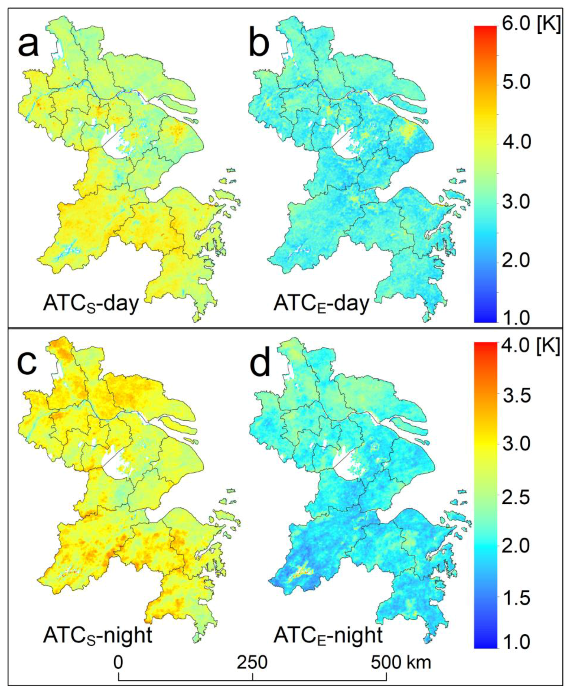
| Land Cover Types | ATCS-Day | ATCE-Day | ATCS-Night | ATCE-Night | Diff-Day | Diff-Night |
|---|---|---|---|---|---|---|
| Grassland | 4.0 | 2.9 | 2.8 | 2.0 | 1.1 | 0.8 |
| Wetland | 3.4 | 2.7 | 2.7 | 2.0 | 0.7 | 0.7 |
| Cropland | 3.7 | 2.8 | 2.9 | 2.1 | 0.9 | 0.8 |
| Built-up | 4.0 | 3.1 | 2.8 | 2.0 | 0.9 | 0.8 |
| Forest | 4.1 | 2.8 | 2.9 | 2.0 | 1.3 | 0.9 |
© 2018 by the authors. Licensee MDPI, Basel, Switzerland. This article is an open access article distributed under the terms and conditions of the Creative Commons Attribution (CC BY) license (http://creativecommons.org/licenses/by/4.0/).
Share and Cite
Zou, Z.; Zhan, W.; Liu, Z.; Bechtel, B.; Gao, L.; Hong, F.; Huang, F.; Lai, J. Enhanced Modeling of Annual Temperature Cycles with Temporally Discrete Remotely Sensed Thermal Observations. Remote Sens. 2018, 10, 650. https://doi.org/10.3390/rs10040650
Zou Z, Zhan W, Liu Z, Bechtel B, Gao L, Hong F, Huang F, Lai J. Enhanced Modeling of Annual Temperature Cycles with Temporally Discrete Remotely Sensed Thermal Observations. Remote Sensing. 2018; 10(4):650. https://doi.org/10.3390/rs10040650
Chicago/Turabian StyleZou, Zhaoxu, Wenfeng Zhan, Zihan Liu, Benjamin Bechtel, Lun Gao, Falu Hong, Fan Huang, and Jiameng Lai. 2018. "Enhanced Modeling of Annual Temperature Cycles with Temporally Discrete Remotely Sensed Thermal Observations" Remote Sensing 10, no. 4: 650. https://doi.org/10.3390/rs10040650