Salient Object Detection via Recursive Sparse Representation

School of Remote Sensing and Information Engineering, Wuhan University, Wuhan 430079, China
*
Author to whom correspondence should be addressed.
Remote Sens. 2018, 10(4), 652; https://doi.org/10.3390/rs10040652
Submission received: 15 March 2018
/
Revised: 12 April 2018
/
Accepted: 19 April 2018
/
Published: 23 April 2018
(This article belongs to the Special Issue Pattern Analysis and Recognition in Remote Sensing)
Abstract
:Object-level saliency detection is an attractive research field which is useful for many content-based computer vision and remote-sensing tasks. This paper introduces an efficient unsupervised approach to salient object detection from the perspective of recursive sparse representation. The reconstruction error determined by foreground and background dictionaries other than common local and global contrasts is used as the saliency indication, by which the shortcomings of the object integrity can be effectively improved. The proposed method consists of the following four steps: (1) regional feature extraction; (2) background and foreground dictionaries extraction according to the initial saliency map and image boundary constraints; (3) sparse representation and saliency measurement; and (4) recursive processing with a current saliency map updating the initial saliency map in step 2 and repeating step 3. This paper also presents the experimental results of the proposed method compared with seven state-of-the-art saliency detection methods using three benchmark datasets, as well as some satellite and unmanned aerial vehicle remote-sensing images, which confirmed that the proposed method was more effective than current methods and could achieve more favorable performance in the detection of multiple objects as well as maintaining the integrity of the object area.

1. Introduction
Visual saliency, which is an important and fundamental research problem in remote-sensing image interpretation, computer vision, psychology and neuroscience, is concerned with the distinct perceptual quality of a biological system that makes certain regions of a scene stand out from their neighbors and thereby helps humans to quickly and accurately focus on the most visually noticeable foreground in a scene [1,2,3,4]. Since the computational model of visual saliency was first introduced [5] and the ensuing expansion of its application [6,7], numerous saliency models have been developed which can be categorized as either bottom-up data-driven methods [8,9,10,11,12,13,14] or task-leading top-down methods [15,16,17]. Bottom-up methods are usually unsupervised, while top-down methods are supervised. The related methods are also categorized as either eye-fixation prediction methods or salient object detection methods [18], depending on the specific needs and objectives. The aim of the eye-fixation prediction methods is to generate a pixel-wise saliency prediction map that is based on a biological model for human eye-fixation activity; the salient object detection methods aim to create a region-level saliency map for the purpose of object appearance preservation [19].
Although the supervised learning-based object detection methods attract great attention and can obtain outstanding results with the booming development of deep-learning technology [20,21,22], there is still enough research value for the unsupervised methods because of their autonomy and adaptability. This work focuses on the unsupervised bottom-up data-driven salient object detection problems. Due to the absence of high-level knowledge, all bottom-up methods rely on assumptions about properties, such as the contrast and compactness of the salient objects and the background. In particular, contrast-based methods [11,23,24,25,26,27] have achieved outstanding performance. However, these methods were designed with heavy contrast feature dependence, which led to some limitations in maintaining the integrity in some cases, including the extraction of entire objects and detection of multiple objects. In addition, the salient object detection tasks can be substantially divided into two processes: (1) object area extraction; and (2) saliency evaluation, to which various image-segmentation, clustering, and graph-optimization methods are applied to improve recognition accuracy. The boundary prior (i.e., image boundary regions are mainly background) is widely used in saliency score computation [28]. Although improved methods have been proposed to enhance the robustness of the boundary constraint [29], its inner shortcomings, which are not completely overcome, may cause detection failure when the salient objects aimed at touch the image boundaries [30].
In general, the limitations of previous salient object detection methods can be summarized as follows, and some examples are presented in Figure 1:
- (1)
- Local contrast methods are designed to solve the local extremum operation problem, in which only the most distinct part of the object tends to be highlighted, while they are unable to uniformly evaluate the saliency of the entire object region.
- (2)
- Global contrast methods aim to capture the holistic rarity of an image so as to improve the deficiency described above for the local contrast methods to a certain extent. However, they continue to be ineffective in comparing different contrast values for the detection of multiple objects, especially those with large dissimilarity.
- (3)
- Boundary prior-based saliency computation may fail when the objects touch the image boundaries.
To solve the above limitations, this paper proposes a new recursive sparse representation (RSR) method, which combines the background reconstructions and foreground ones; treats the reconstruction errors as the saliency indicator, avoiding the integrity shortcomings of contrast-based methods and the weak robustness of boundary prior-based methods with the following major contributions.
- (1)
- Both background and foreground dictionaries are generated and the currently separated reconstructions are combined to enhance the stability of sparse representation.
- (2)
- The traditional eye-fixation results [5] are introduced to extract the initial background and foreground dictionaries. Compared with the previous related methods such as [31] which only use the boundary prior, the proposed RSR method is expected to be more robust, especially for the images with salient objects that touch the boundaries.
- (3)
- A recursive processing step is utilized to optimize the final detection results and weaken the dependence on the initial saliency map obtained from eye-fixation results.
After presenting a literature review of the related bottom-up methods in Section 1.1, the algorithmic outline is described in Section 1.2. Section 2 is dedicated to the details of the proposed method, and in Section 3 the proposed method is evaluated against the seven current state-of-the-art methods on three benchmark datasets and remote-sensing images. In Section 4, the conclusions of this study and recommendations for future work are introduced.
1.1. Related Works
This paper specifically focuses on unsupervised bottom-up data-driven salient object detection; therefore, only the most influential related works are reviewed in this section and compared in the experiments.
1.1.1. The Previous Saliency Detection Methods
As mentioned previously, the bottom-up methods always rely on some assumptions about the properties of the target objects and the useless background regions, for which the contrast prior is widely used in various existing methods. Since Koch et al. [34] set up the foundation of visual saliency and Itti et al. [4] proposed a local color contrast method based on the “center-surround difference” school of thought, many related methods that consider multiple-feature integration or optimization with extra constraints have been introduced such as the graph-based visual saliency method (GBVS) [35], or the Markov chain-absorbed method (MC) [36] as well as some newer methods [14,37,38,39,40]. Of late, the global contrast-based methods have attracted a great interest in light of the commonly known drawbacks of the local contrast-based methods that may limit them to only be able to detect high-contrast edges while missing the inside of a salient object.
Achanta et al. [10] detected the salient region with frequency domain contrast. Perazzi et al. [12] utilized high-dimensional Gaussian filters and the variance of spatial distribution for each color to evaluate saliency. Cheng et al. [11,33] proposed a simple and efficient saliency extraction algorithm based on regional contrast, which simultaneously evaluated the global appearance contrast and spatial coherence. However, the results of global contrast-based methods in terms of contrast comparison show that the drawbacks of their multiple object-detection methods continue to be recognized. Saliency detection, after all, is conducted for the purpose of computing the saliency scores of all the image pixels and generating a saliency map. Whether for local or global contrast-based methods, an appropriate salient measure is always a crucial factor. Center prior and boundary prior are the two most widely used measures for saliency score computation [18,41,42]. The former assumes that the regions close to the image center are more likely to receive a higher saliency score, while the latter assumes that the regions which touch the image boundaries will get a lower score. However, the ever-accumulating research and experimental results, contradictory to the above assumptions, continue to confirm that the detection may easily fail when the salient objects touch the image boundaries.
In order to improve the situation, more robust boundary prior strategies have been proposed and used to enhance the reliability of saliency computation [29,30]. Following the idea that salient object detection is a combination of region segmentation and saliency evaluation, [19] proposed a novel recursive clustering-based method and reported competitive results for multiple object detection. Moreover, there are several proposed methods based on sparse-low rank decomposition [43,44,45], which regard the salient regions as the sparse items, and methods based on sparse representation which made full use of the difference between the background and foreground [31,44,45].
1.1.2. Saliency Detection and Remote Sensing
Saliency detection is essentially similar to the target recognition and extraction in remote sensing. According to the eye fixation or some specific task requirements, the interested objects in the image are extracted. However, traditional saliency detection is commonly applied to nature images, while little related research in remote sensing exists. With the common development of image-processing and remote-sensing technology, saliency detection methods have spread and extended in the field of remote sensing. Much research has combined the physiological characteristics of human vision and image interpretation to complete specific object detection, such as ship detection [7], building detection [46,47,48], and cloud extraction [49], etc. Besides, remote-sensing image classification is also a direction of the application of saliency detection theory [21,50].
In addition, with the development of extensive remote-sensing data, problems about data accumulation and redundancy are unavoidable. Saliency detection, the way to recognize the areas that attract attention and are effective, can be further developed as a means of data compression and data screening in remote sensing.
1.2. The Proposed Approach
As described in previous studies [36,51], it is a reasonable assumption that there must be a large difference between the reconstruction errors of the foreground and background regions using the same dictionary in sparse representation. Thus, the opposite two regions can be effectively divided by their errors. Once the background and foreground regions are used as the dictionaries, the reconstruction errors can directly indicate the salient level of the regions.
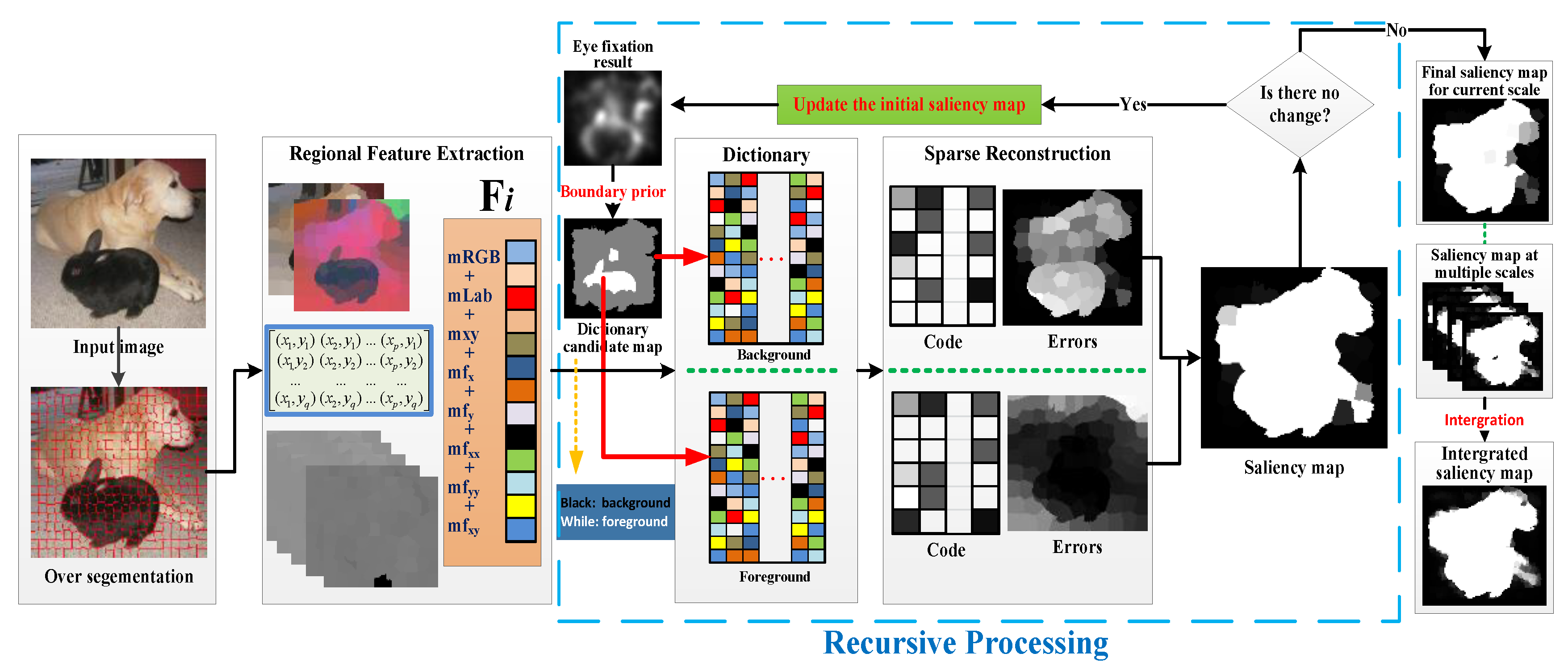
The framework of the proposed RSR method is shown in Figure 2. To better capture structural information, the superpixels are generated, using the simple linear iterative clustering (SLIC) algorithm [52] to segment an input image into multiple uniform and compact regions, which are treated as the base units of processing. Note that only one scale with 400 superpixels is presented in Figure 2 to simplify the expression. For the regions at each scale, a traditional eye-fixation result is introduced as the initial saliency map, which is combined with the boundary prior to extract the background and foreground regions (i.e., reconstruction dictionaries). Following regional feature extraction, all the image regions are reconstructed and their saliency scores (saliency map) are calculated by the two groups’ reconstruction errors. Then, the initial saliency map is updated by the latest saliency map and the proposed sparse representation stages are repeated until a significant change between the current and last saliency maps cannot be detected.
2. Methodology
2.1. Regional Feature Extraction
Given an input image, it is first over-segmented by the SLIC algorithm, which can reduce the number of regions for computation with minimal information loss and better capture of the structural information. For each region, the proposed features consist of the color, spatial and geometric information. Each color space has its own specific advantages. RGB is an additive color system based on trichromatic theory and is non-linear with visual perception. CIE Lab is designed to approximate human vision and has been widely used for salient region detection [24,26,27,53]. RGB and Lab color are combined in the proposed RSR method. In addition, the location information is added to restrict the spatial range of the region interactions, and the first order and second order gradients are used to describe the detailed information. Eventually, each pixel of the image is represented with a 13-dimensional feature vector as , where and are the three components of the RGB and Lab colors respectively; are the image coordinates of the pixel; and are the first and second gradients of the pixel. Then, the mean feature of the pixels in each superpixel is used to describe the region as , and the entire segmented image is represented as , where is the number of regions, is the feature dimension, and all the feature values are normalized.
2.2. Background and Foreground-Based Sparse Representation
Many previous studies have shown the image boundaries’ high performance and the sparse representation’s feasibility in saliency detection [18]. However, the previous DSR study revealed that the solutions (i.e., coefficients) obtained by sparse representation are less stable, especially if it is based on the boundary background constraint, which has inherent shortcomings. The proposed method combines the background and foreground dictionaries to complete the detection task by sparse representation in order to alleviate these disadvantages.
2.3. Dictionary Building
There are two separate sparse representation processing steps in this study: background-based and foreground-based. Both dictionaries are mainly concerned with regions (superpixels) generation and representations, namely, the elements in the former are regions related to background and the latter contains foreground regions. The process is described in detail for regional feature extraction in Section 2.1. The background and foreground dictionaries are respectively set as and , where is the number of background regions and is the foreground regions. Unlike DSR, the eye-fixation result is introduced to determine the elements in and in the proposed RSR method. It is known that regions attracting higher attention are more likely to be the foreground, whereas the opposite is true for the background. The eye-fixation result is used to restrict the extraction of background regions for adaption to cases with salient objects touching the boundaries, and it is the basis for foreground dictionary building. and are determined by Equation (1) and a detection example with different dictionaries is shown in Figure 3. The whole process of dictionary-building is as follows:
- (1)
- Extracting regions which touch the image boundaries as ;
- (2)
- Calculating the regional fixation level by averaging the value of the region pixels and setting the result as , where is the number of regions and is the eye-fixation level value of region ;
- (3)
- Setting a coefficient of proportionality , and taking the first smaller elements as , the first larger elements as .
2.4. Salient Object Detection by Sparse Representation
Sparse coding generally means that a given regional feature vector can be expressed as a sparse linear combination of dictionary elements, and it is reasonable to assume that the background and foreground regions will yield a large number of different reconstruction errors based on the same dictionary.
Given background dictionary and foreground dictionary , image region is encoded by Equations (2) and (3), and the reconstruction errors which can directly and reverse directly indicate the salient level of the regions are calculated by Equations (4) and (5).
where , is the sparse code vector obtained by dictionaries and ; , are the regularization parameters that are empirically set to 0.01 in the experiment referred to DSR; , are the reconstruction errors as a result of the background and foreground sparse representation.
As shown in Figure 2, whether the region is salient or not is expressed in opposite ways in the two error maps. As described in DSR, the errors caused by background-based sparse representation can directly measure the saliency so the foreground-based reconstruction errors can work in the opposite way. In this paper, the region saliency map is simply calculated according to Equation (6), upon which the pixel saliency map then is easily computed following the criteria that the pixels in the same region hold the same saliency. The question of whether other methods could achieve better results by using Equation (6) is not discussed in this paper.
where is the saliency value of region , is a regulatory factor that is set to 0.1.
2.5. Recursive Processing and Integrated Saliency Map Generation
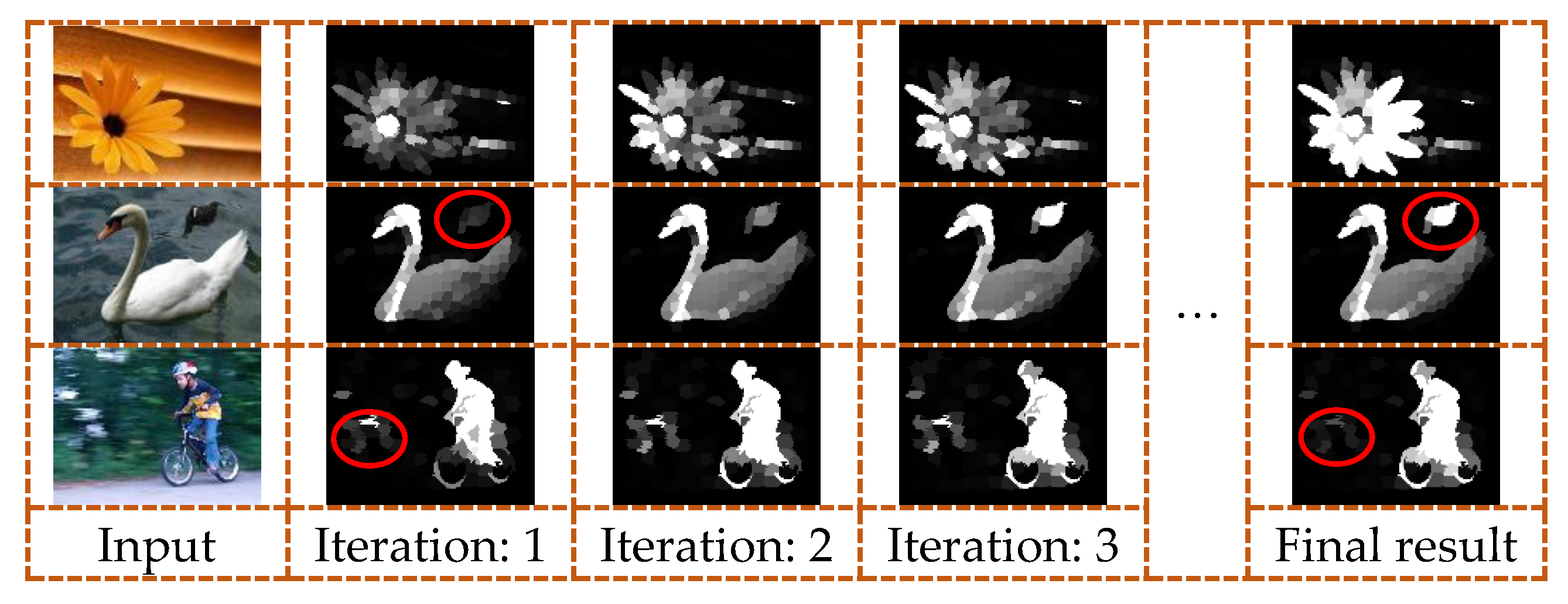
It was found that the performance of the sparse representation can be significantly controlled by its dictionary quality and, therefore, can directly determine the saliency detection results (Figure 3) in the proposed RSR method. Since the dictionary is extracted with the initial saliency map, namely, the eye-fixation result only, the detection accuracy is highly dependent on the fixation results. Aiming to weaken the shortcomings of the above dependency, a simple recursive process was constructed around the initial saliency map to optimize the results. The effectiveness of the optimization is apparent in the visualization results of Figure 4. The pseudocode of the recursive processing is described as Algorithm 1.
| Algorithm 1 | |
| 1. | Input: three bands color image I |
| 2. | Output: final saliency map FSM |
| 3. | S = super-pixel-segmentation (I) //over segmentation |
| 4. | Regional feature FS = {F1, F2,…, FN} //Fi = [R, G, B, L, a, b, x, y, fx, fy, fxx, fyy, fxy] regional mean |
| 5. | Initial saliency map ISM = IT eye fixation result //regional mean, initialization |
| 6. | Repeat{ |
| 7. | 1) Boundary prior + ISM => Db, Df // dictionary extraction, |
| 8. | // Db is the background dictionary and Df is the foreground dictionary |
| 9. | 2) Db + Fs → Errb & Errf // Sparse representation |
| 10. | // Errb and Errf are reconstruction errors based on Db and Df |
| 11. | 3) Errb/(Errf + a) → current saliency map CSM // a is a small positive decimal |
| 12. | 4) If CSM ≌ ISM (The similarity is compared to RPcorr) then repeat break |
| 13 | else repeat continue end |
| 14 | 5) If Number of repeats < Threshold |
| 15. | thenISM = CSM and continue |
| 16 | else repeat break end} |
| 17. | FSM = Last (CSM) |
| 18. | ReturnFSM |
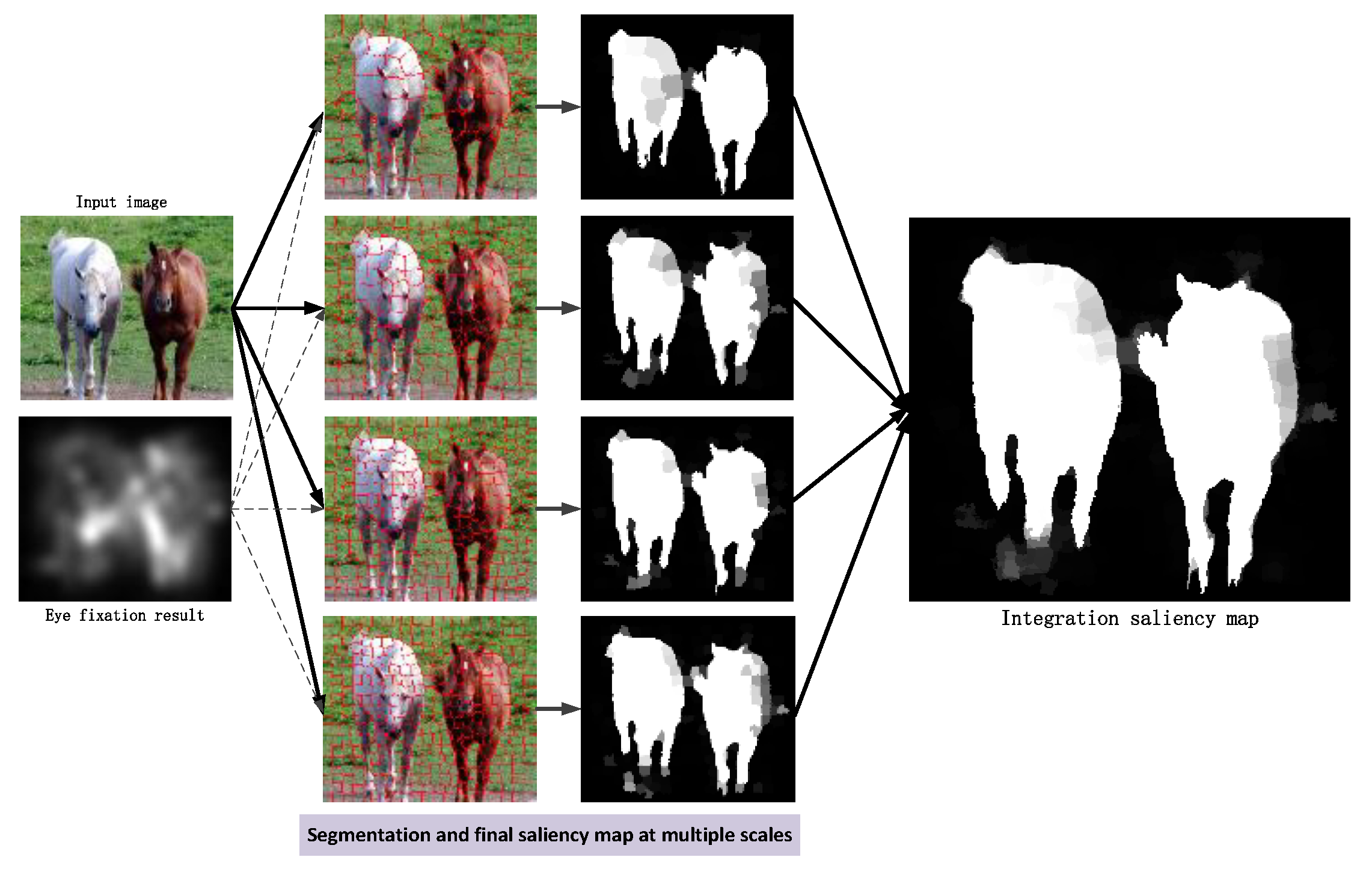
To handle the scale problem, the superpixels at different scales were generated by setting the multiple number parameters of the SLIC algorithm empirically as 100, 200, 300, and 400 in the proposed RSR method, which were commonly used in many previous studies. After the multiple scale recursive processing, was obtained and the final saliency map of the proposed RSR method was integrated by averaging the multiscale results. The integration is illustrated in Figure 5.
3. Experimental Results and Analysis
In this section, the performance of the proposed RSR method is evaluated by comparing it to the following seven state-of-the-art saliency detection algorithms: IT [5], the contrast-aware saliency detection (CA) [8], HC [33], MC [36], RBD [29], recursive regional feature clustering model (RRFC) [19], and DSR [31]. The evaluation measures were analyzed in the benchmark [18], which contained the curve, the curve, and the mean absolute error (), and were used for quantitative comparisons. All the measures are detailed in Section 3.2. The up-arrow after a measure indicates that the larger the value achieved, the better the performance; while the down-arrow indicates the smaller, the better. It is noted that, for a binary mask, was used to represent the number of non-zero entries in the mask.
3.1. Datasets
Three benchmark datasets about the close range images which are widely used in saliency detection research were chosen as the experiment’s data, including MSRA-ASD [33], SED2 [23], and ECSSD [27]. MRSA-ASD contains 1000 single object images with a pixel-wise ground truth. SED2 consists of 100 images that contain exactly two objects, and the pixel-wise ground truth is also provided. In particular, there are enormous challenges in this dataset due to the dissimilarity between the objects and the fact that objects are touching the image border. In addition, ECSSD contains a large number of semantically meaningful but structurally complex natural images.
As little saliency research in remote-sensing images has been undertaken, there are no classical testing datasets with existing ground truth. Two categories of Chinese high-spatial resolution satellite (GF-1) and unmanned aerial vehicle (UAV) images are introduced to evaluate the effectiveness and novelty of the proposed method in remote sensing, and the manual-detection results are used as the reference. The detailed parameters of these images are provided in Table 1.
3.2. Evaluation Measures
(1) : is defined as the percentage of salient pixels correctly assigned, while is the ratio of correctly detected salient pixels to all true salient pixels. The curve is created by varying the saliency threshold, which determines whether a pixel belongs to the salient object. For a saliency map , it can be converted to a binary mask , so that its and Equation (7) can be computed by comparing with ground truth . When a binarization map is completed with a fixed threshold that changes from 0 to 1, a group pair of precision-recall values is computed and a curve can be formed.
(2) is a weighted harmonic mean of and to comprehensively evaluate the quality of a saliency map, Equation (8).
where is the non-negative weight and is commonly set to 0.3.
(3) is a similarity score between and that is defined as following equation:
where is the image width while is the height, and the mask and are normalized from 0 to 1.
3.3. Experimental Parameter Settings
All the parameters of the state-of-the-art methods were set by default in the original published literatures for all the experiments, and some of the key factors of the proposed RSR method are summarized in Table 2.
3.4. Visual Comparison on the Benchmark Datasets
Figure 6 displays the visual comparisons between the proposed RSR method and the seven state-of-the-art existing methods on the three benchmark datasets. It is apparent in Figure 6 that the proposed RSR method, for the specific datasets in the experiments, successfully extracted accurate entire salient objects, regardless of whether they were single objects, multiple objects, or even images with complex structures. For the single object, the eye-fixation (IT) and the traditional contrast-based methods (CA, HC) only produced fuzzy contours, while the improved methods clearly obtained better results (MC, RBD, RRFC and DSR), and the proposed RSR performed best. In terms of the multiple objects, the proposed RSR method obtained good results, and in these cases only a few of the state-of-the-art methods could deal with such objects with large dissimilarities and saliency differences. In Figure 6, for the images with complex structure or similarity between the background and the foreground, such as the second image of MSRA-ASD, the second of SED2 and all the images in ECSSD, the results show that the proposed RSR method exhibited greater detection capability. Therefore, the proposed RSR method not only provides good results for single object detection, but also obviously works better for extracting multiple objects and maintaining the saliency consistency of the entire objects than the other state-of-the-art methods.
3.5. Quantitative Comparison on the Benchmark Datasets
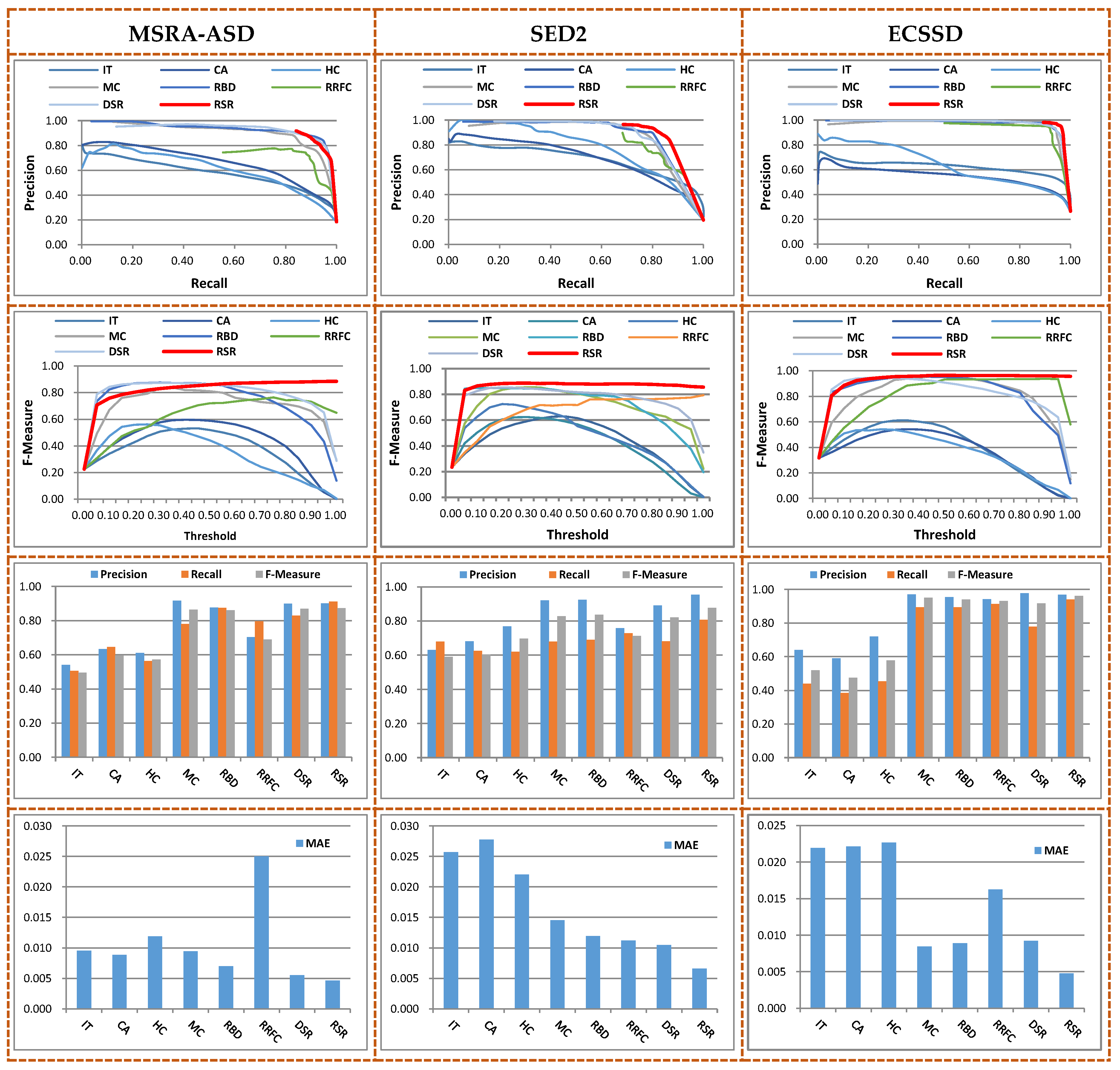
The quantitative comparison between the proposed RSR method and the seven state-of-the-art methods was completed with curve, and measure. Figure 7 shows the evaluations on the MSRA-ASD, SED2 and ECSSD datasets.
In terms of the curve and , the proposed RSR method performed quite competitively with the latest improved methods, such as RBD, RRFC, and DSR, which are considered to be the outstanding performers in the seven state-of-the-art methods utilized in the experiments. At the same time, the three measures of the proposed RSR method were more balanced and stable, while the compared state-of-the-art methods always had at least one measure value with a relatively low index. With respect to , the proposed RSR method’s performance was obviously better in the comparisons, no matter for the situations of the single object, the multiple objects, or the images that were structurally complex.
For the MSRA-ASD dataset, the proposed RSR method uniformly highlighted the salient regions and adequately suppressed the backgrounds from the lowest and higher recall value. Although the of the proposed RSR method was slightly lower than the best state-of-the-art method, its results fully demonstrated the superiority of the proposed RSR method in maintaining the accuracy of the saliency and the integrity of the object.
For the SED2 dataset that contained images with multiple objects, and the ECSSD dataset, which contained structurally-complex images, the advantages of the proposed RSR method also were more apparent; in particular, the new RRFC technique, which uses recursive clustering to improve the accuracy of multi-object detection in order to obtain a relatively higher recall value and to ensure that enough salient objects can be detected. However, the proposed RSR method can achieve a higher precision and recall, and its effectiveness at solving a grim detection challenge is also proved.
3.6. Comparison of Results on the Remote-Sensing Datasets
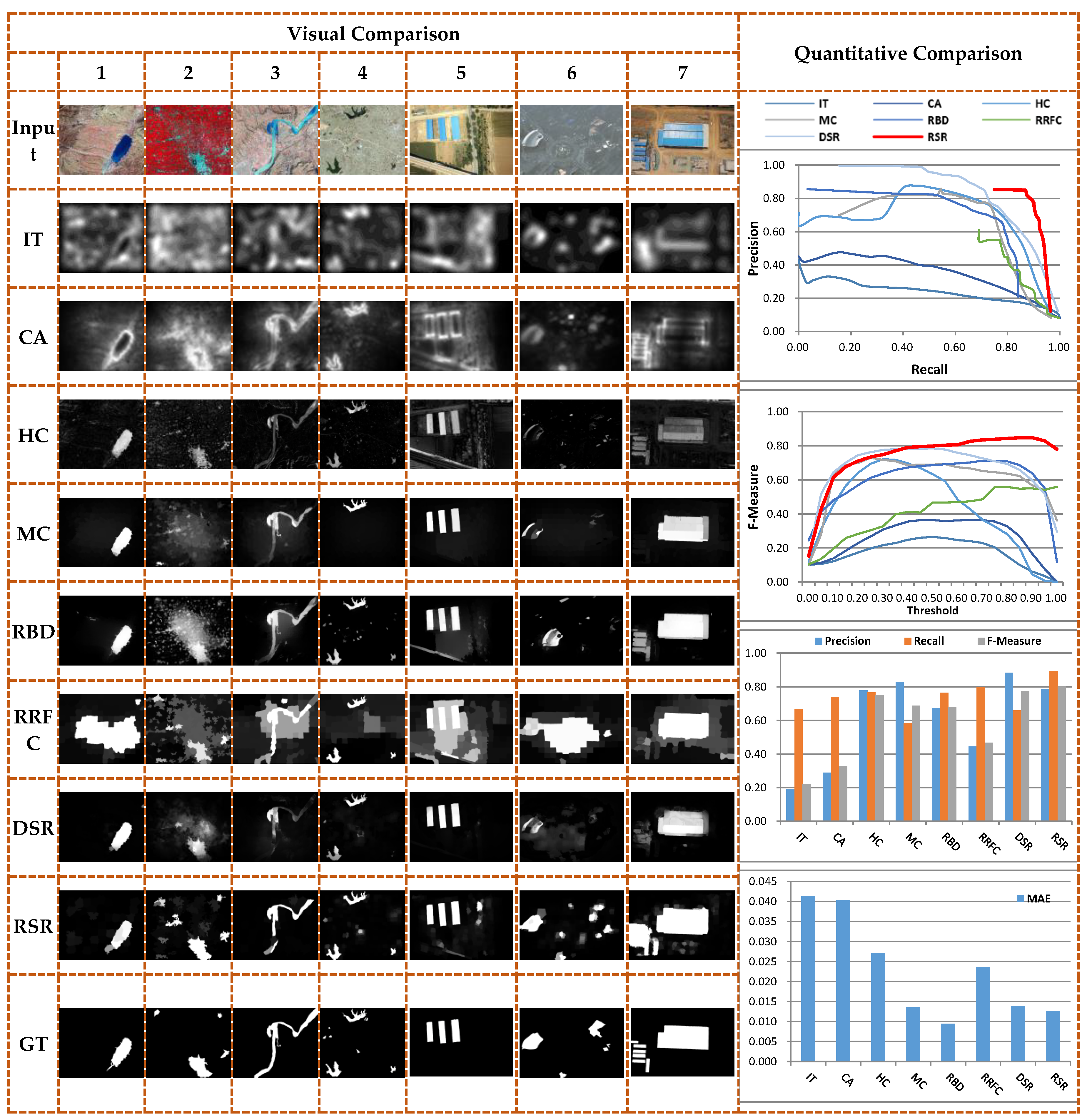
Figure 8 displays the comparisons between the proposed RSR method and the seven state-of-the-art existing methods on the GF-1 and UAV remote-sensing images, where the visual results are similar to those in Figure 6. It is apparent that for the traditional eye-fixation and contrast-based methods it was difficult to ensure the integrity of the objects. For a clear salient object, whether it is a building or a water area, the improved methods could successfully obtain accurate entire results just like the RSR did. However, when the aimed object was the area composed of small subblocks (such as the second image in Figure 8), the RSR performed relatively better in the experiments. From the point of view of the quantitative analysis, the RSR also worked well in weighting the relationship between the and , and could obtain a lower result, which is the quantification of its ability to maintain the saliency consistency and keep the object integrity.
3.7. Limitations and Shortcomings
The proposed method exploits the sparse representations based on background and foreground dictionaries which are mainly initially determined by a combination of the boundary prior and eye-fixation results. To a greater or lesser extent, the input information has a certain impact on the detection results. Although the recursive processing is introduced for optimization, there shortcomings with regard to highlighting some salient areas with weak eye fixation or when they touch the image edges (see the first row of Figure 1, where this issue is described as an edge limitation). In addition, the saliency results of the proposed RSR method are simply evaluated using Equation (6) to reduce computation expense, which may lead to over-detection (i.e., highlighting the background to a certain extent). The results with shortcomings of the benchmark datasets are shown in Figure 9.
As for remote-sensing images, it is easy to find that all the experimental methods faced an ability reduction. Although the ground truth generated by hand lacks validation and might weaken the reliability of the evaluation, it can also help in the completion of the comparison analysis. In terms of Figure 8, there is an over-detection shortcoming of the proposed RSR, whereby some small areas in the complex environment background were given a high salient level and detected.
4. Conclusions
This paper presented an efficient salient object detection method that uses recursive sparse representation and combines the background and foreground dictionaries. The reconstruction errors, which can reflect the similarity between the target units and the dictionaries, are used as the salient indicator; and a recursive processing operation acts as an optimization step.
The experimental results on three benchmark datasets about close-range images show that the proposed RSR method performed better than the seven state-of-the-art methods that it was compared with. RSR also was shown to be capable of working more effectively and efficiently on the multiple objects and the images with complex structures, which was represented by its ability to maintain a uniform and integrated salient object area. As for the results on GF-1 and UAV images, these help to confirm that the proposed RSR could work relatively better in remote sensing than state-of-art methods, and its potential was also proved.
In terms of the limitations of the proposed RSR method, the salient results obtained by sparse representation were reliant on the dictionaries that were initially built based on the boundary prior and initial saliency map; and while the final calculations are simple and require the input of only a few factors, future work should focus on further generalizing the proposed RSR method by the integration of more background and foreground constraints. In addition, the effectiveness of the proposed RSR in remote sensing is not fully confirmed in these limited experiments, and so it ought to be further developed and widely tested on more remote-sensing data as well to improve and adapt it to different fields of remote sensing.
Acknowledgments
This research was partially supported by the National Natural Science Foundation of China under Grants 41322010 and 41571434.
Author Contributions
Yongjun Zhang and Xiang Wang conceived of the study and designed the experiments. Xunwei Xie and Yansheng Li took part in the research. Xiang Wang wrote the main program and most of the paper.
Conflicts of Interest
The authors declare no conflict of interest.
References
- Borji, A.; Itti, L. State-of-the-art in visual attention modeling. IEEE Trans. Pattern Anal. Mach. Intell. 2013, 35, 185–207. [Google Scholar] [CrossRef] [PubMed]
- Borji, A.; Sihite, D.N.; Itti, L. Quantitative analysis of human model agreement in visual saliency modeling: A comparative study. IEEE Trans. Image Process. 2013, 22, 55–69. [Google Scholar] [CrossRef] [PubMed]
- Hayhoe, M.; Ballard, D. Eye movements in natural behavior. Trends Cognit. Sci. 2005, 9, 188–194. [Google Scholar] [CrossRef] [PubMed]
- Itti, L.; Koch, C. Computational modelling of visual attention. Nature Rev. Neurosci. 2001, 2, 194–203. [Google Scholar] [CrossRef] [PubMed]
- Itti, L.; Koch, C.; Niebur, E. A model of saliency-based visual attention for rapid scene analysis. IEEE Trans. Pattern Anal. Mach. Intell. 1998, 20, 1254–1259. [Google Scholar] [CrossRef]
- Xiang, D.L.; Tang, T.; Ni, W.P.; Zhang, H.; Lei, W.T. Saliency Map Generation for SAR Images with Bayes Theory and Heterogeneous Clutter Model. Remote Sens. 2017, 9, 1290. [Google Scholar] [CrossRef]
- Dong, C.; Liu, J.H.; Xu, F. Ship Detection in Optical Remote Sensing Images Based on Saliency and a Rotation-Invariant Descriptor. Remote Sens. 2018, 10, 400. [Google Scholar] [CrossRef]
- Goferman, S.; Zelnik-Manor, L.; Tal, A. Context-aware saliency detection. IEEE Trans. Pattern Anal. Mach. Intell. 2012, 32, 1915–1925. [Google Scholar] [CrossRef] [PubMed]
- Jiang, H.Z.; Wang, J.D.; Yuan, Z.J.; Liu, T.; Zheng, N.N.; Li, S.P. Automatic salient object segmentation based on context and shape prior. BMVC 2011, 6, 9–20. [Google Scholar]
- Achanta, R.; Hemami, S.; Estrada, F.; Susstrunk, S. Frequency-tuned salient region detection. In Proceedings of the IEEE Conference on Computer Vision and Pattern Recognition, Miami, FL, USA, 20–25 June 2009; pp. 1597–1604. [Google Scholar]
- Cheng, M.M.; Zhang, G.X.; Mitra, N.J.; Huang, X.L.; Hu, S.M. Global contrast based salient region detection. In Proceedings of the IEEE Conference on Computer Vision and Pattern Recognition, Colorado Springs, CO, USA, 20–25 June 2011; pp. 569–582. [Google Scholar]
- Perazzi, F.; Krahenbuhl, P.; Pritch, Y.; Hornung, A. Saliency filters: Contrast based filtering for salient region detection. In Proceedings of the IEEE Conference on Computer Vision and Pattern Recognition, Providence, RI, USA, 16–21 June 2012; pp. 733–740. [Google Scholar]
- Lu, Y.; Zhang, W.; Lu, H.; Xue, X.Y. Salient object detection using concavity context. In Proceedings of the IEEE International Conference on Computer Vision, Barcelona, Spain, 6–13 November 2011; pp. 233–240. [Google Scholar]
- Yang, C.; Zhang, L.H.; Lu, H.C. Graph-regularized saliency detection with convex-hull-based center prior. IEEE Signal Process. Lett. 2013, 20, 637–640. [Google Scholar] [CrossRef]
- Borji, A. Boosting bottom-up and top-down visual features for saliency estimation. In Proceedings of the IEEE Conference on Computer Vision and Pattern Recognition, Providence, RI, USA, 16–21 June 2012; pp. 438–445. [Google Scholar]
- Yang, J.M.; Yang, M.H. Top-down visual saliency via joint crf and dictionary learning. In Proceedings of the IEEE Conference on Computer Vision and Pattern Recognition, Providence, RI, USA, 16–21 June 2012; pp. 2296–2303. [Google Scholar]
- Liu, T.; Yuan, Z.J.; Sun, J.; Wang, J.D.; Zheng, N.N.; Tang, X.O.; Shum, H.Y. Learning to detect a salient object. IEEE Trans. Pattern Anal. Mach. Intell. 2011, 33, 353–367. [Google Scholar] [PubMed]
- Borji, A.; Cheng, M.M.; Jiang, H.Z.; Li, J. Salient Object Detection: A Benchmark. IEEE Trans. Image Proc. 2015, 24, 5706–5722. [Google Scholar] [CrossRef] [PubMed]
- Ohm, K.; Lee, M.; Lee, Y.; Kim, S. Salient object detection using recursive regional feature clustering. Inf. Sci. 2017, 387, 1–18. [Google Scholar]
- Hu, P.; Shuai, B.; Liu, J.; Wang, G. Deep level sets for salient object detection. In Proceedings of the IEEE Conference on Computer Vision and Pattern Recognition, Honolulu, HI, USA, 21–26 July 2017; pp. 2300–2309. [Google Scholar]
- Gong, X.; Xie, Z.; Liu, Y.Y.; Shi, X.G.; Zheng, Z. Deep salient feature based anti-noise transfer network for scene classification of remote sensing imagery. Remote Sens. 2018, 10, 410. [Google Scholar] [CrossRef]
- Hou, Q.B.; Cheng, M.M.; Hu, X.W.; Borji, A.; Tu, Z.W.; Torr, P.H.S. Deeply supervised salient object detection with short connections. In Proceedings of the IEEE Conference on Computer Vision and Pattern Recognition, Honolulu, HI, USA, 21–26 July 2017; pp. 3203–3212. [Google Scholar]
- Alpert, S.; Galun, M.; Basri, R.; Brant, A. Image segmentation by probabilistic bottom-up aggregation and cue integration. In Proceedings of the IEEE Conference on Computer Vision and Pattern Recognition, Minneapolis, MN, USA, 17–22 June 2007; pp. 1–8. [Google Scholar]
- Jiang, H.Z.; Wang, J.D.; Yuan, Z.J.; Wu, Y.; Zheng, N.N.; Li, S.P. Salient object detection: A discriminative regional feature integration approach. In Proceedings of the IEEE Conference on Computer Vision and Pattern Recognition, Portland, OR, USA, 23–28 June 2013; pp. 2083–2090. [Google Scholar]
- Li, Z.C.; Qin, S.Y.; Itti, L. Visual attention guided bit allocation in video compression. Image Vis. Comput. 2011, 29, 1–14. [Google Scholar] [CrossRef]
- Oh, K.H.; Lee, M.; Kim, G.; Kim, S. Detection of multiple salient objects through the integration of estimated foreground clues. Image Vis. Comput. 2016, 54, 31–44. [Google Scholar] [CrossRef]
- Shi, J.P.; Yan, Q.; Xu, L.; Jia, J.Y. Hierarchical image saliency detection on extended CSSD. IEEE Trans. Pattern Anal. Mach. Intell. 2015, 38, 717–729. [Google Scholar] [CrossRef] [PubMed]
- Wei, Y.C.; Wen, F.; Zhu, W.J.; Sun, J. Geodesic saliency using background priors. In Proceedings of the European Conference on Computer Vision, Florence, Italy, 7–13 October 2012; pp. 29–42. [Google Scholar]
- Zhu, W.J.; Liang, S.; Wei, Y.C.; Sun, J. Saliency optimization from robust background detection. In Proceedings of the IEEE Conference on Computer Vision and Pattern Recognition, Columbus, OH, USA, 23–28 June 2014; pp. 2814–2821. [Google Scholar]
- Li, H.; Wu, E.H.; Wu, W. Salient region detection via locally smoothed label propagation with application to attention driven image abstraction. Neurocomputing 2017, 230, 359–373. [Google Scholar] [CrossRef]
- Li, X.H.; Lu, H.C.; Zhang, L.H.; Ruan, X.; Yang, M.S. Saliency detection via dense and sparse reconstruction. In Proceedings of the IEEE International Conference on Computer Vision, Sydney, NSW, Australia, 1–8 December 2013; pp. 2976–2983. [Google Scholar]
- Achanta, R.; Estrada, F.; Wils, P.; Süsstrunk, S. Salient region detection and segmentation. In Proceedings of the International Conference on Computer Vision Systems, Santorini, Greece, 12–15 May 2008; pp. 66–75. [Google Scholar]
- Cheng, M.M.; Mitra, N.J.; Huang, X.L.; Torr, P.H.S.; Hu, S.M. Global contrast based salient region detection. IEEE Trans. Pattern Anal. Mach. Intell. 2015, 37, 569–582. [Google Scholar] [CrossRef] [PubMed]
- Koch, C.; Ullman, S. Shifts in selective visual attention: Towards the underlying neural circuitry. Hum. Neurobiol. 1985, 4, 219–227. [Google Scholar] [PubMed]
- Harel, J.; Koch, C.; Perona, P. Graph-based visual saliency. In Proceedings of the Advances in neural Information Processing Systems, Vancouver, BC, Canada, 4–5 December 2006; pp. 545–552. [Google Scholar]
- Jiang, B.W.; Zhang, L.H.; Lu, H.C.; Yang, C.; Yang, M.S. Saliency detection via absorbing markov chain. In Proceedings of the IEEE International Conference on Computer Vision, Sydney, NSW, Australia, 1–8 December 2013; pp. 1665–1672. [Google Scholar]
- Chen, J.Z.; Ma, B.P.; Cao, H.; Chen, J.; Fan, Y.B.; Li, R.; Wu, W.M. Updating initial labels from spectral graph by manifold regularization for saliency detection. Neurocomputing 2017, 266, 79–90. [Google Scholar] [CrossRef]
- Zhang, J.X.; Ehinger, K.A.; Wei, H.K.; Zhang, K.J.; Yang, J.Y. A novel graph-based optimization framework for salient object detection. Pattern Recognit. 2017, 64, 39–50. [Google Scholar] [CrossRef]
- He, Z.Q.; Jiang, B.; Xiao, Y.; Ding, C.; Luo, B. Saliency detection via a graph based diffusion model. In Proceedings of the International Workshop on Graph-Based Representations in Pattern Recognition, Anacapri, Italy, 16–18 May 2017; pp. 3–12. [Google Scholar]
- Yan, Q.; Xu, L.; Shi, J.P.; Jia, J.Y. Hierarchical saliency detection. In Proceedings of the IEEE Conference on Computer Vision and Pattern Recognition, Portland, OR, USA, 23–28 June 2013; pp. 1155–1162. [Google Scholar]
- Judd, T.; Durand, F.; Torralba, A. A Benchmark of Computational Models of Saliency to Predict Human Fixations; Technical Report; Creative Commons: Los Angeles, CA, USA, 2012. [Google Scholar]
- Borji, A.; Sihite, D.N.; Itti, L. Salient object detection: A benchmark. In Proceedings of the European Conference on Computer Vision, Florence, Italy, 7–13 October 2012; pp. 414–429. [Google Scholar]
- Peng, H.W.; Li, B.; Ling, H.B.; Hu, W.M.; Xiong, W.H.; Maybank, S.J. Salient object detection via structured matrix decomposition. IEEE Trans. Pattern Anal. Mach. Intell. 2017, 39, 818–832. [Google Scholar] [CrossRef] [PubMed]
- Zhang, L.B.; Lv, X.R.; Liang, X. Saliency analysis via hyperparameter sparse representation and energy distribution optimization for remote sensing images. Remote Sens. 2017, 9, 636. [Google Scholar] [CrossRef]
- Hu, Z.P.; Zhang, Z.B.; Sun, Z.; Zhao, S.H. Salient object detection via sparse representation and multi-layer contour zooming. IET Comput. Vis. 2017, 11, 309–318. [Google Scholar] [CrossRef]
- Tan, Y.H.; Li, Y.S.; Chen, C.; Yu, J.G.; Tian, J.W. Cauchy graph embedding based diffusion model for salient object detection. JOSA A 2016, 33, 887–898. [Google Scholar] [CrossRef] [PubMed]
- Li, Y.S.; Tan, Y.H.; Deng, J.J.; Wen, Q.; Tian, J.W. Cauchy graph embedding optimization for built-up areas detection from high-resolution remote sensing images. IEEE J. Sel. Top. Appl. Earth Obs. Remote Sens. 2015, 8, 2078–2096. [Google Scholar] [CrossRef]
- Brunner, D.; Lemoine, G.; Bruzzone, L.; Brunner, D.; Lemoine, G.; Bruzzone, L. Earthquake damage assessment of buildings using VHR optical and SAR imagery. IEEE Trans. Geosci. Remote Sens. 2010, 48, 2403–2420. [Google Scholar] [CrossRef]
- Tan, K.; Zhang, Y.J.; Tong, X. Cloud extraction from chinese high resolution satellite imagery by probabilistic latent semantic analysis and object-based machine learning. Remote Sens. 2016, 8, 963. [Google Scholar] [CrossRef]
- Patra, S.; Bruzzone, L. A novel SOM-SVM-based active learning technique for remote sensing image classification. IEEE Trans. Geosci. Remote Sens. 2014, 52, 6899–6910. [Google Scholar] [CrossRef]
- Duan, L.J.; Wu, C.P.; Miao, J.; Qing, L.Y.; Fu, Y. Visual saliency detection by spatially weighted dissimilarity. In Proceedings of the IEEE Conference on Computer Vision and Pattern Recognition, Colorado Springs, CO, USA, 20–25 June 2011; pp. 473–480. [Google Scholar]
- Achanta, R.; Shaji, A.; Smith, K.; Lucchi, A.; Fua, P.; Susstrunk, S. SLIC superpixels compared to state-of-the-art superpixel methods. IEEE Trans. Pattern Anal. Mach. Intell. 2012, 34, 2274–2282. [Google Scholar] [CrossRef] [PubMed]
- Oh, K.H.; Kim, S.H.; Kim, Y.C.; Lee, Y.R. Detection of multiple salient objects by categorizing regional features. KSII Trans. Internet Inf. Syst. 2016, 10, 272–287. [Google Scholar]
Figure 1.
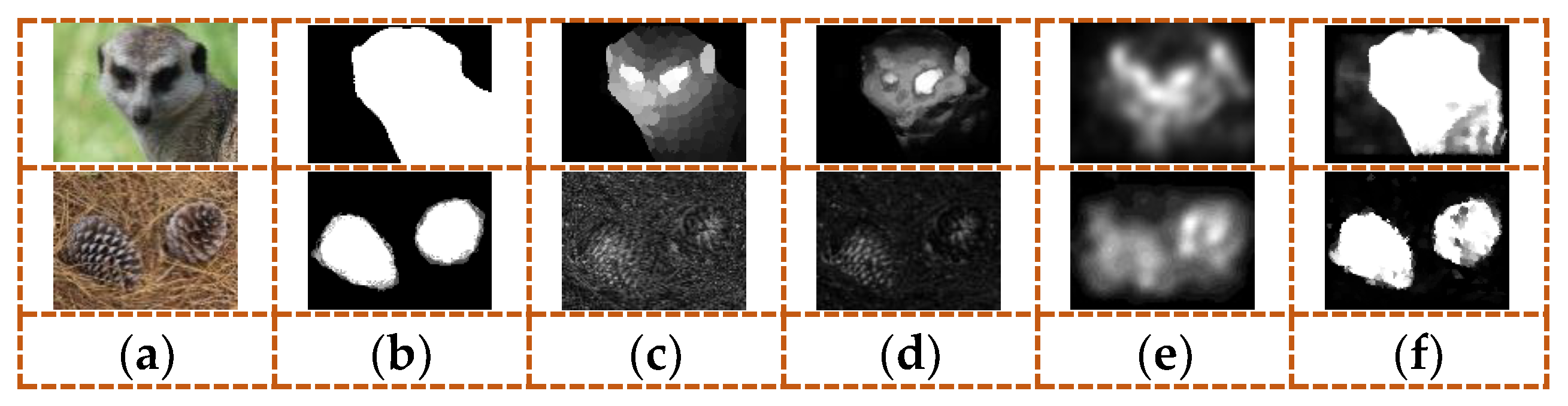
Examples of the limitations of previous contrast and boundary prior-based methods. The images in the first row are the examples of boundary prior testing: (a) input; (b) ground truth; (c) saliency map of saliency optimization from robust background detection (RBD) [29] using boundary prior; (d) saliency map of dense and spares reconstruction based method (DSR) [31] related to boundary prior; (e) initial saliency map of the proposed recursive sparse representation (RSR) generated by Itti’s visual attention model (IT) [5]; (f) final saliency map of the proposed RSR. The images in the second row are the examples of contrast prior testing: (a) input; (b) ground truth; (c) saliency map of low level-features of luminance and color based method (AC) [32] related to local contrast; (d) saliency map of histogram-based contrast method (HC) [33] related to global contrast; (e) initial saliency map of the proposed RSR generated by IT [5]; (f) final saliency map of the proposed RSR.
Figure 1.
Examples of the limitations of previous contrast and boundary prior-based methods. The images in the first row are the examples of boundary prior testing: (a) input; (b) ground truth; (c) saliency map of saliency optimization from robust background detection (RBD) [29] using boundary prior; (d) saliency map of dense and spares reconstruction based method (DSR) [31] related to boundary prior; (e) initial saliency map of the proposed recursive sparse representation (RSR) generated by Itti’s visual attention model (IT) [5]; (f) final saliency map of the proposed RSR. The images in the second row are the examples of contrast prior testing: (a) input; (b) ground truth; (c) saliency map of low level-features of luminance and color based method (AC) [32] related to local contrast; (d) saliency map of histogram-based contrast method (HC) [33] related to global contrast; (e) initial saliency map of the proposed RSR generated by IT [5]; (f) final saliency map of the proposed RSR.

Figure 2.
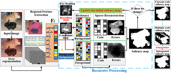
The framework of the proposed approach. Only one scale of SLIC segmentation is illustrated in detail.
Figure 2.
The framework of the proposed approach. Only one scale of SLIC segmentation is illustrated in detail.

Figure 3.
Saliency results based on different dictionaries: (a) input image; (b) ground truth; (c) IT fixation result; (d) saliency result by RSR with background-based sparse representation only; (e) saliency result by RSR with foreground-based sparse representation and background-based sparse representation without saliency map restricting the dictionary extraction; (f) saliency result by complete RSR. Judging from the two groups of the experiments shown in (e,f), the foreground-based combined methods can get an obviously better result when compared to the single representation by background dictionary as shown in (d).

Figure 4.
Examples of recursive processing.

Figure 5.
Integration of multiscale results.

Figure 6.
Visual comparison on MRSA-ASD, ECSSD and SED2 datasets, where GT represents the ground truth.
Figure 6.
Visual comparison on MRSA-ASD, ECSSD and SED2 datasets, where GT represents the ground truth.

Figure 7.
Quantitative comparison results on MSRA-ASD, SED2 and ECSSD datasets. The first row is curve; the second row is curve; the third row is the , and values with adaptive threshold; and the last row is the measure value with adaptive threshold.
Figure 7.
Quantitative comparison results on MSRA-ASD, SED2 and ECSSD datasets. The first row is curve; the second row is curve; the third row is the , and values with adaptive threshold; and the last row is the measure value with adaptive threshold.

Figure 8.
Comparison of the remote sensing dataset. In the right side, the first three graphs are the , and values with adaptive threshold; and the last one is the measure value with adaptive threshold.
Figure 8.
Comparison of the remote sensing dataset. In the right side, the first three graphs are the , and values with adaptive threshold; and the last one is the measure value with adaptive threshold.

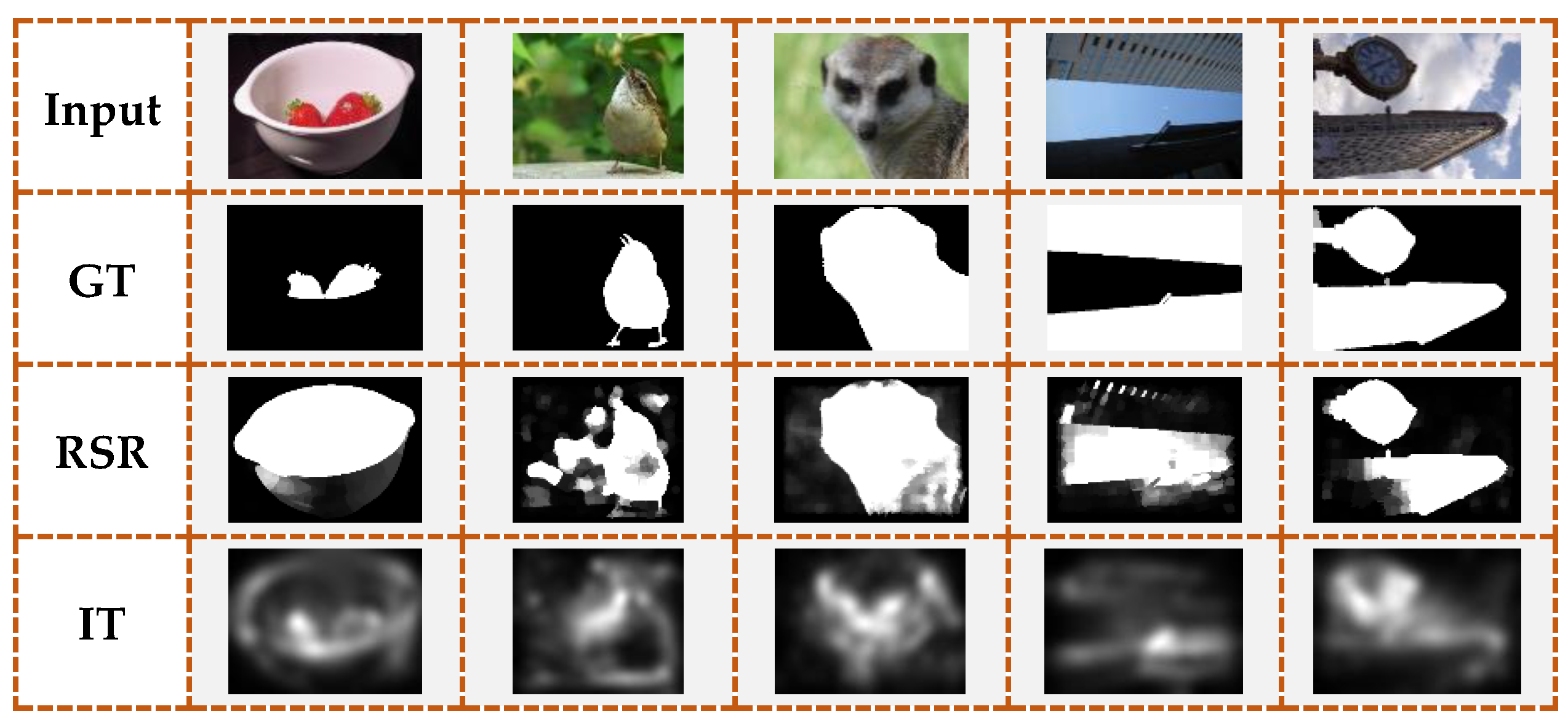
Figure 9.
Some results with shortcomings of the proposed RSR in benchmark datasets. Columns 1 and 2 are over-detections and columns 3–5 are edge limitations.
Figure 9.
Some results with shortcomings of the proposed RSR in benchmark datasets. Columns 1 and 2 are over-detections and columns 3–5 are edge limitations.


Table 1.
Overview of Chinese GF-1 and UAV multispectral datasets.
| Image Parameters | GF-1 | UAV |
|---|---|---|
| Product level | 1A | Original image |
| Number of bands | 4 | 3 |
| Spatial resolution (m) | 8 | 0.6 |
| Original image size | 4548 × 500 | 6000 × 4000 |
| Experimental image cutting size | 1000 × 800 | 1000 × 666 |
| Land-cover type | Buildings + mountains + water | Buildings |
Table 2.
Parameters of the proposed RSR method.
| Parameter | Value | Remark |
|---|---|---|
| 100, 200, 300, 400 | Superpixel number of the SLIC segmentation | |
| 0.2 | Coefficient of proportionality in dictionary extraction | |
| 0.01 | Regularization parameters in sparse representation | |
| 0.1 | Regulatory factor in saliency map computation | |
| 0.3 | Weight value in PR computation | |
| 0.9999 | Similarity coefficient threshold in recursive processing | |
| 10 | Iteration times, upper threshold in recursive processing | |
| 3 | Iteration times, lower threshold in recursive processing |
© 2018 by the authors. Licensee MDPI, Basel, Switzerland. This article is an open access article distributed under the terms and conditions of the Creative Commons Attribution (CC BY) license (http://creativecommons.org/licenses/by/4.0/).
Share and Cite
MDPI and ACS Style
Zhang, Y.; Wang, X.; Xie, X.; Li, Y. Salient Object Detection via Recursive Sparse Representation. Remote Sens. 2018, 10, 652. https://doi.org/10.3390/rs10040652
AMA Style
Zhang Y, Wang X, Xie X, Li Y. Salient Object Detection via Recursive Sparse Representation. Remote Sensing. 2018; 10(4):652. https://doi.org/10.3390/rs10040652
Chicago/Turabian StyleZhang, Yongjun, Xiang Wang, Xunwei Xie, and Yansheng Li. 2018. "Salient Object Detection via Recursive Sparse Representation" Remote Sensing 10, no. 4: 652. https://doi.org/10.3390/rs10040652
Note that from the first issue of 2016, this journal uses article numbers instead of page numbers. See further details here.