Characterizing the Spatio-Temporal Pattern of Land Surface Temperature through Time Series Clustering: Based on the Latent Pattern and Morphology


Abstract
:
1. Introduction
2. Study Area and Data Sets
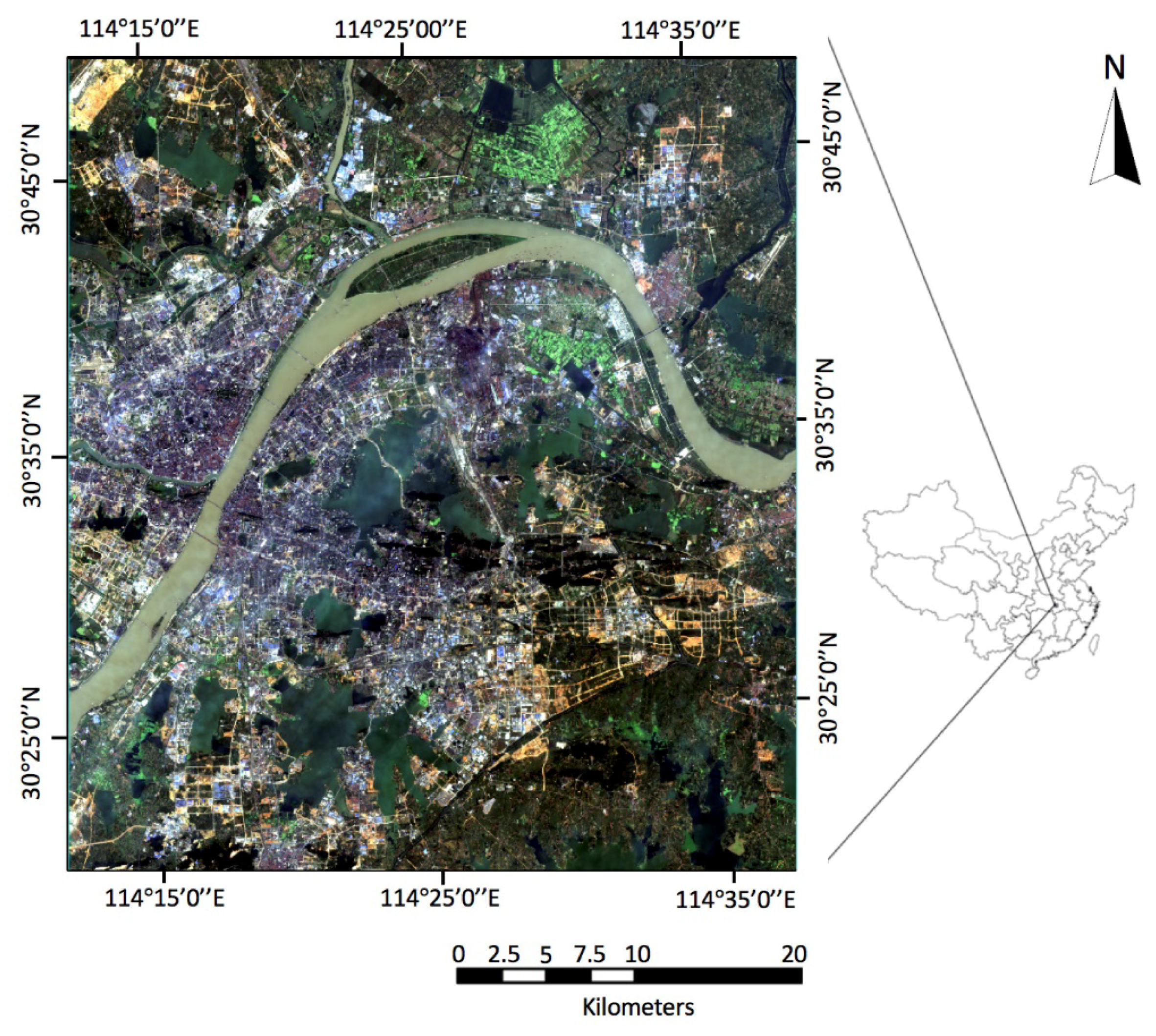
2.1. Wuhan, China
2.2. Data Sets
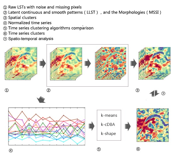
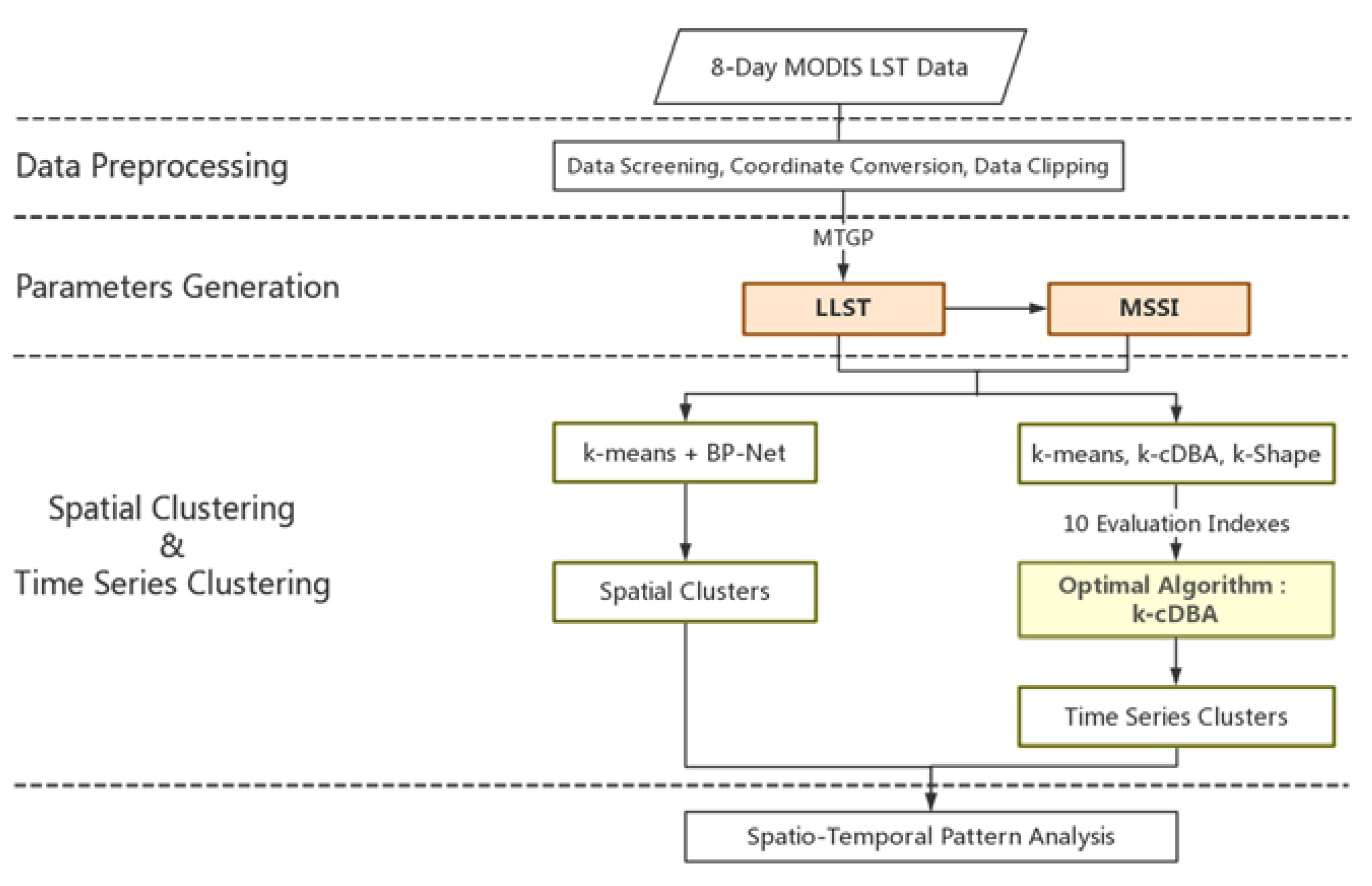
3. Methodology
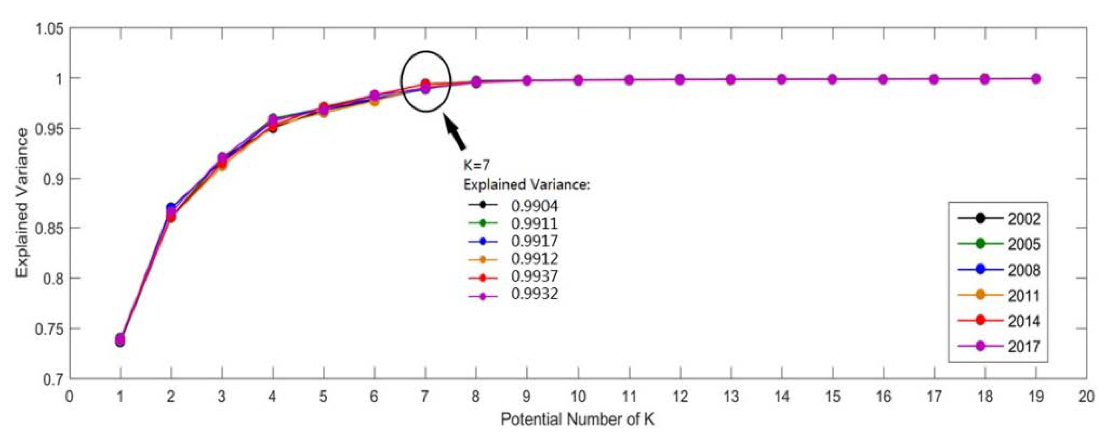
3.1. The Latent Pattern of LST
3.2. The Morphology
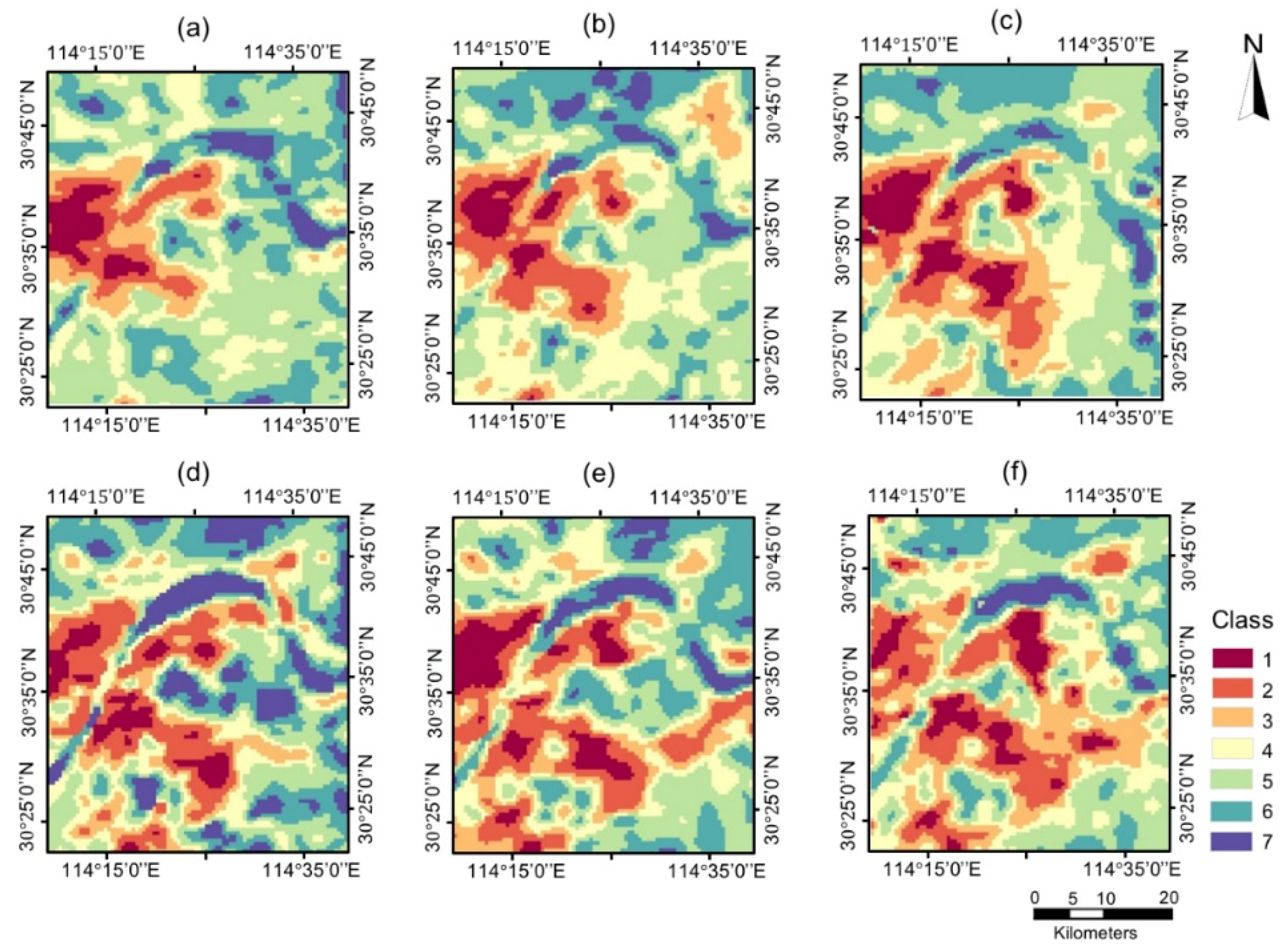
3.3. The Spatial Pattern
3.4. The Spatio-Temporal Pattern
4. Results
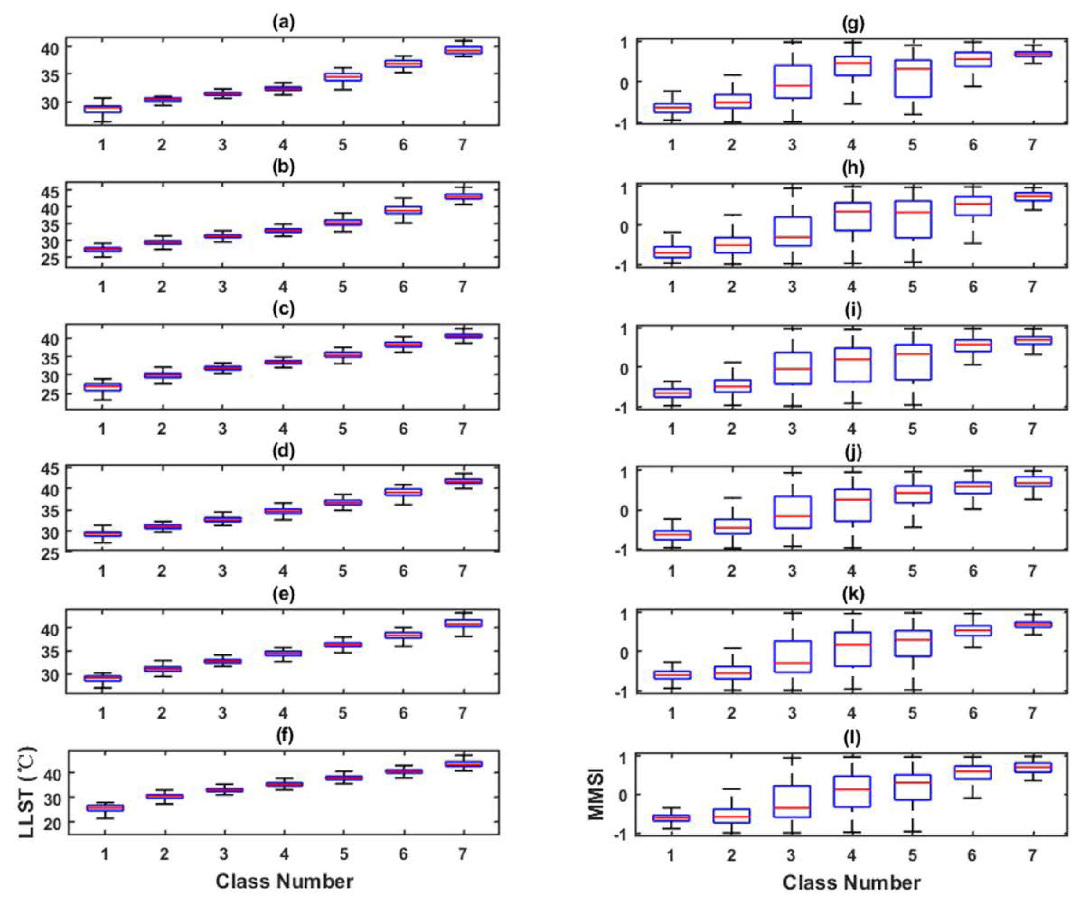
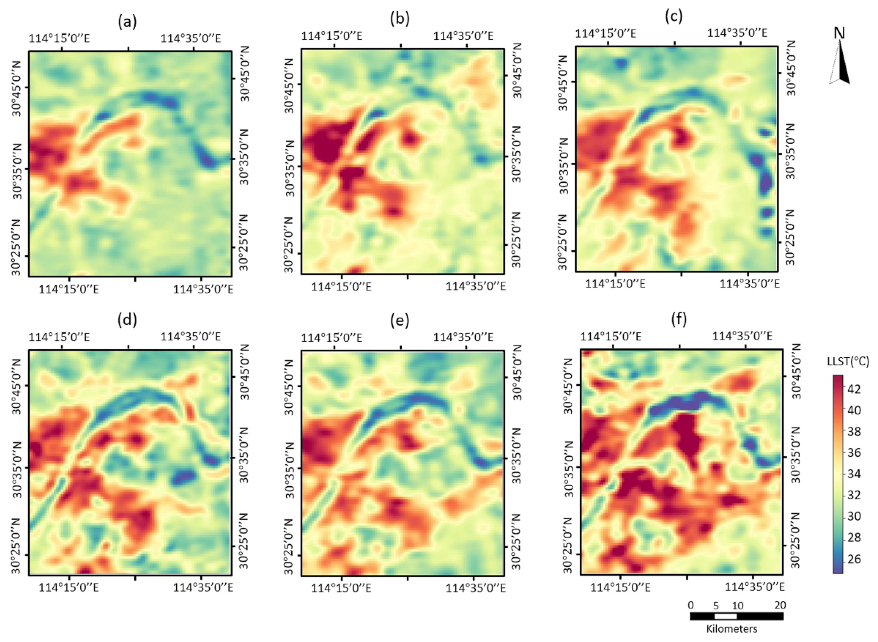
4.1. The LLST Patterns
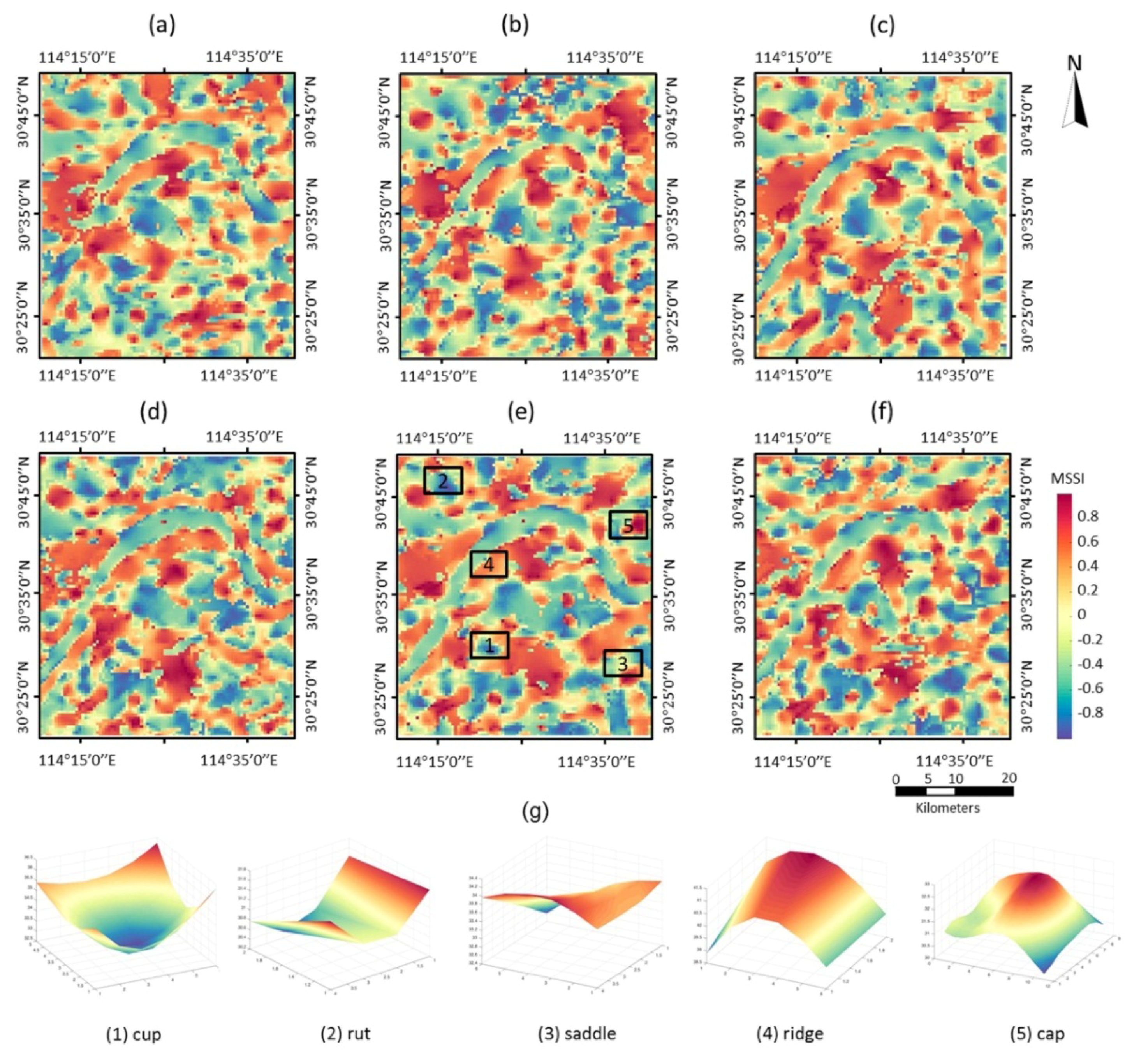
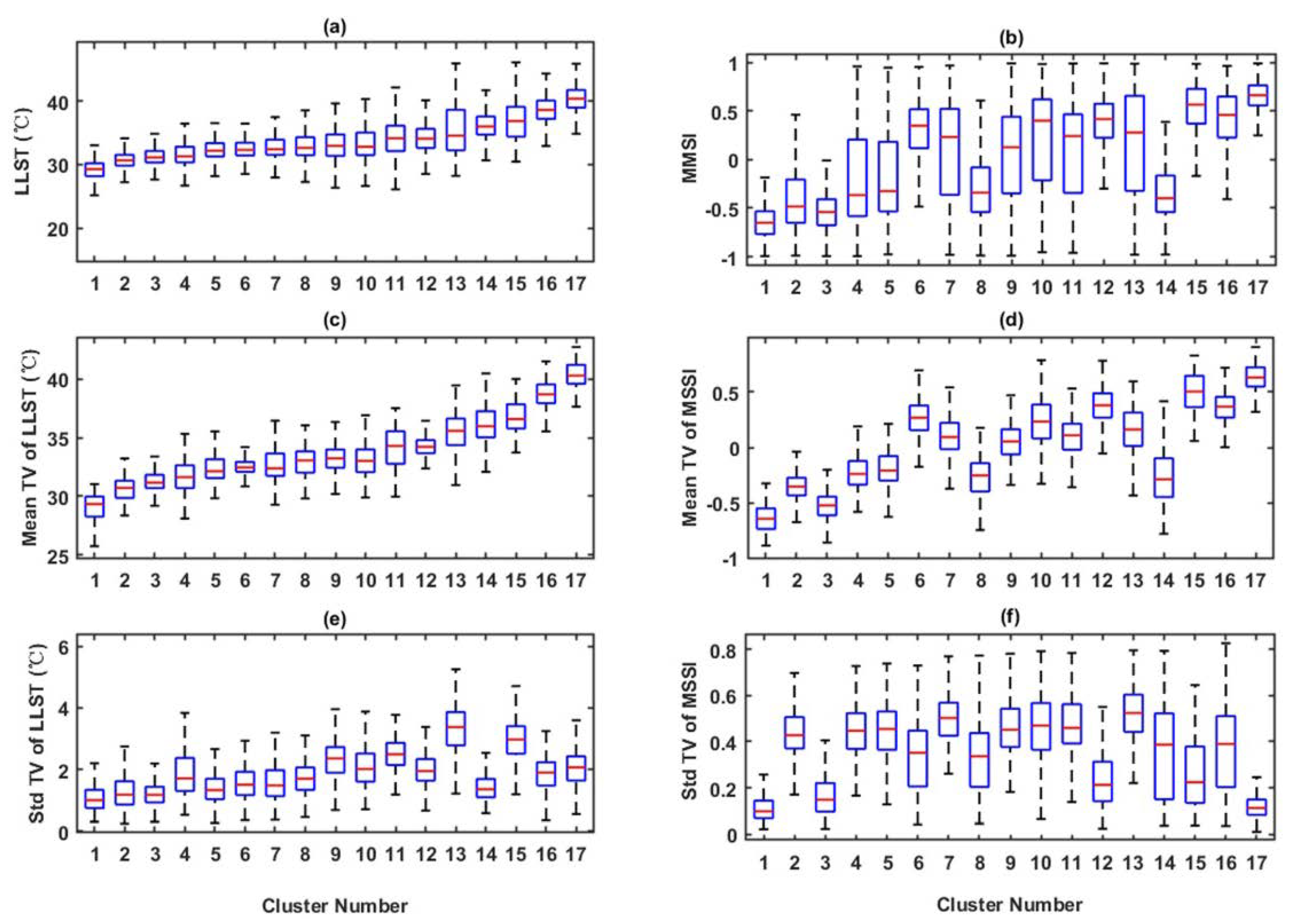
4.2. The Morphological Characteristics of LLSTs
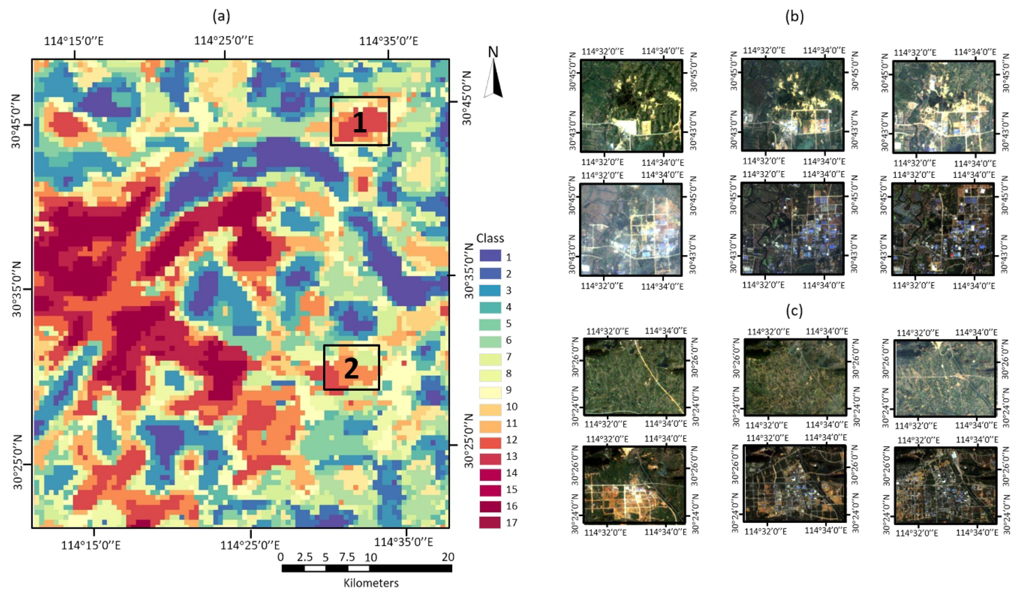
4.3. The Spatial Patterns
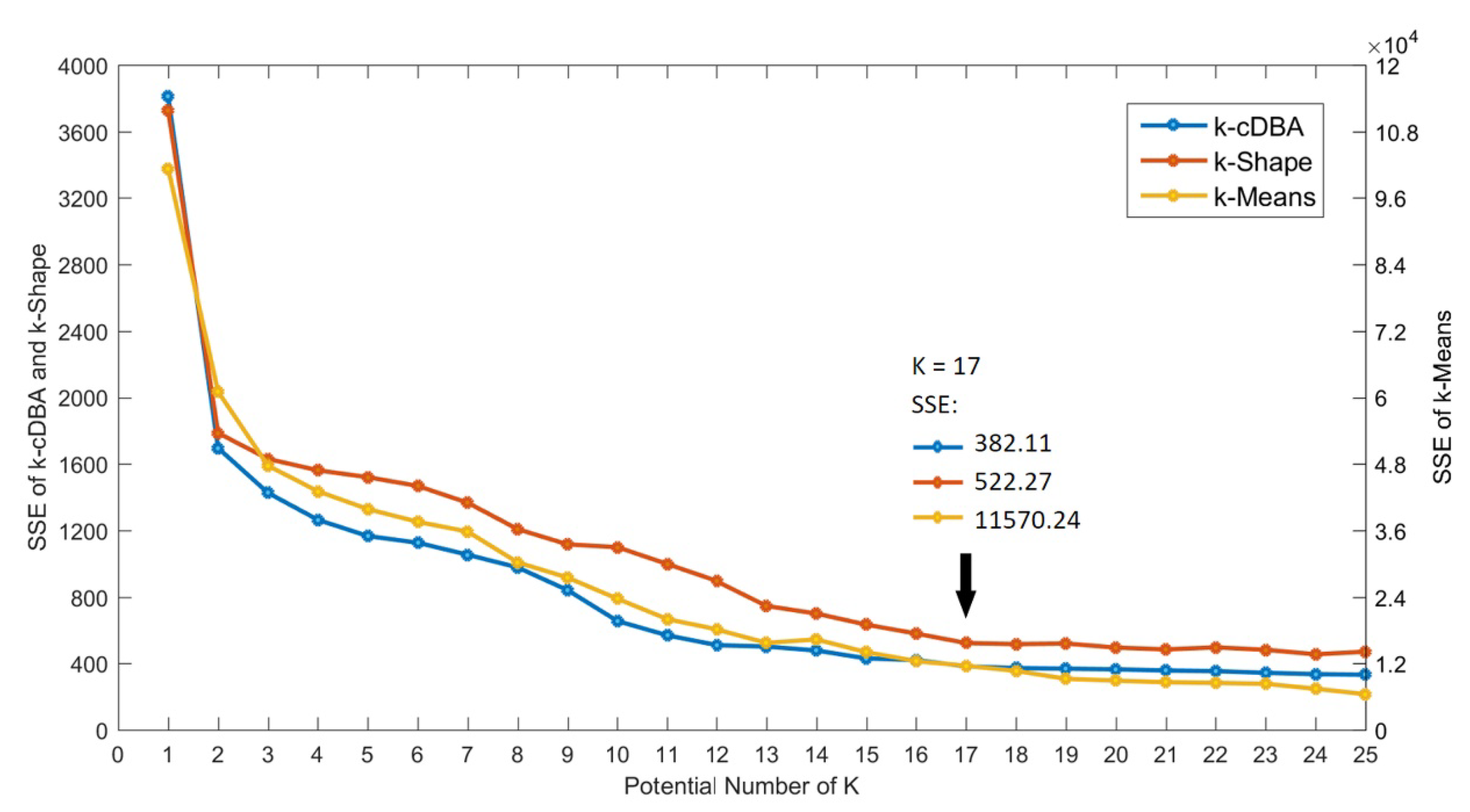
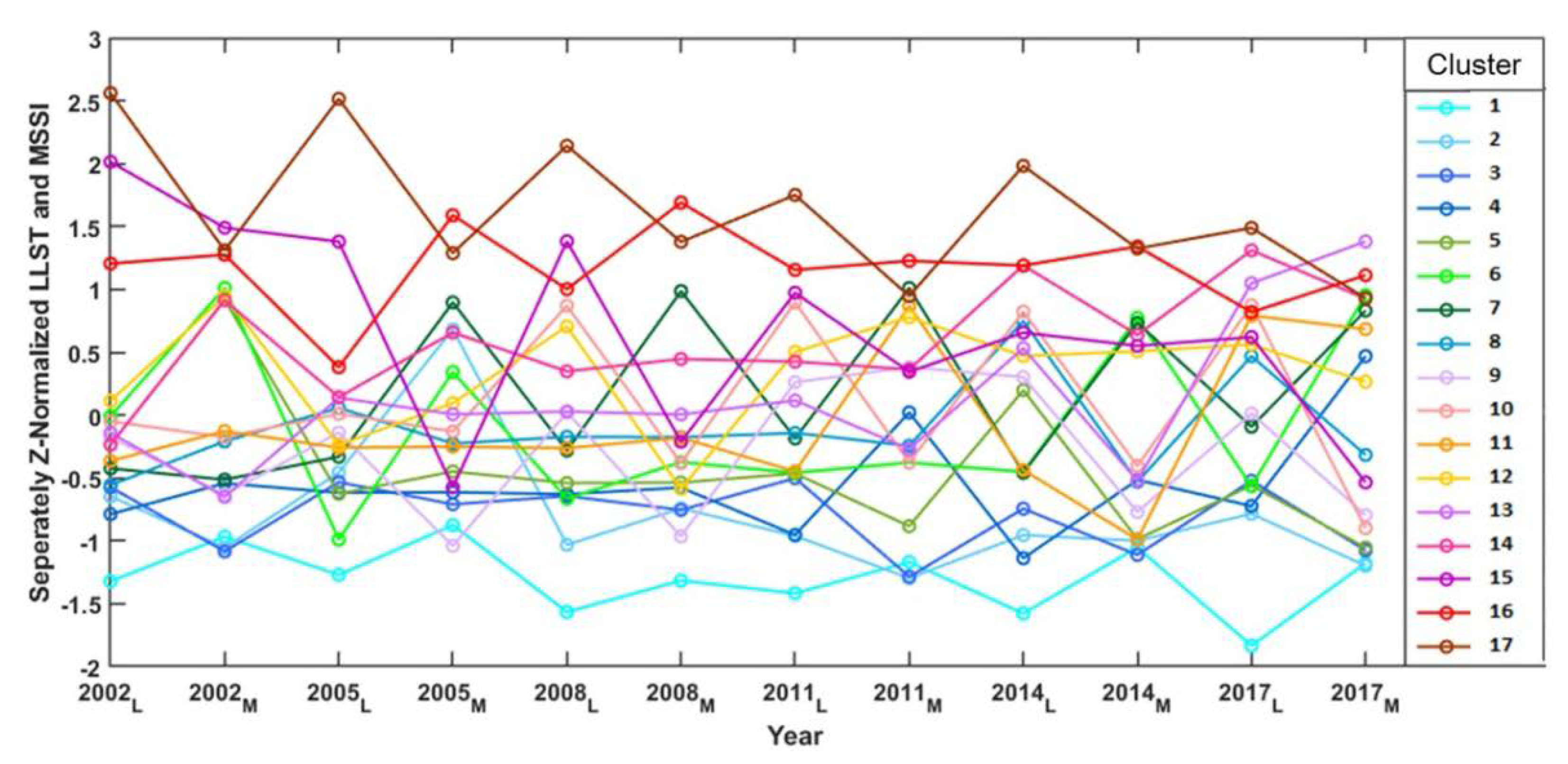
4.4. The Spatio-Temporal Pattern
5. Discussion
6. Conclusions
Acknowledgments
Author Contributions
Conflicts of Interest
Abbreviations
| ARD | Automatic Relevance Determinant |
| ARI | Adjusted Rand Index |
| BP-Net | Back-Propagation Neural Networks |
| CC | Correlation Coefficient |
| cDTW | The Constrained Dynamic Time Warping |
| CSM | Cluster Similarity Measure |
| DBA | the Dynamic Time Warping Baryleft Averaging |
| ED | Euclidean Distance |
| FM | Folkes and Mallow index |
| GP | Gaussian Process |
| k-cDBA | Time Series Clustering Algorithm with c-DTW as the Distance Measure, and DBA for Centroid Computation |
| LCZ | Local Climate Zone |
| LST | Land Surface Temperature |
| LLST | Latent Pattern of LST |
| LULC | Land Use and Land Cover |
| MODIS | MODerate-resolution Imaging Spectroradiometer |
| MTGP | Multi-Task Gaussian Process Modeling |
| MSSI | Multi-Scale Shape Index |
| NMI | Normalized Mutual Information |
| RI | Rand Index |
| SI | The Shape Index |
| SSE | Sum of Squared Error |
| Std | Standard Deviation |
| TIR | Thermal Infrared |
References
- Weng, Q. Thermal infrared remote sensing for urban climate and environmental studies: Methods, applications, and trends. ISPRS J. Photogramm. Remote Sens. 2009, 64, 335–344. [Google Scholar] [CrossRef]
- Weng, Q.; Fu, P. Modeling annual parameters of clear-sky land surface temperature variations and evaluating the impact of cloud cover using time series of landsat tir data. Remote Sens. Environ. 2014, 140, 267–278. [Google Scholar] [CrossRef]
- Fu, P.; Weng, Q. A time series analysis of urbanization induced land use and land cover change and its impact on land surface temperature with Landsat imagery. Remote Sens. Environ. 2016, 175, 205–214. [Google Scholar] [CrossRef]
- Stewart, I.D.; Oke, T.R. Local climate zones for urban temperature studies. Bull. Am. Meteorol. Soc. 2012, 93, 1879–1900. [Google Scholar] [CrossRef]
- Weng, Q.; Lu, D.; Schubring, J. Estimation of land surface temperature–vegetation abundance relationship for urban heat island studies. Remote Sens. Environ. 2004, 89, 467–483. [Google Scholar] [CrossRef]
- Chen, X.; Zhao, H.; Li, P.; Yin, Z. Remote sensing image-based analysis of the relationship between urban heat island and land use/cover changes. Remote Sens. Environ. 2006, 104, 133–146. [Google Scholar] [CrossRef]
- Song, J.; Du, S.; Feng, X.; Guo, L. The relationships between landscape compositions and land surface temperature: Quantifying their resolution sensitivity with spatial regression models. Landsc. Urban Plan. 2014, 123, 145–157. [Google Scholar] [CrossRef]
- Wang, J.; Zhan, Q.; Guo, H.; Jin, Z. Characterizing the spatial dynamics of land surface temperature–impervious surface fraction relationship. Int. J. Appl. Earth Obs. Geoinf. 2016, 45, 55–65. [Google Scholar] [CrossRef]
- Andrienko, G.; Andrienko, N.; Demšar, U.; Dransch, D.; Dykes, J.; Fabrikant, S.; Jern, M.; Kraak, M.; Schumann, H.; Tominski, C. Space, time and visual analytics. Int. J. Geogr. Inf. Sci. 2010, 24, 1577–1600. [Google Scholar] [CrossRef]
- Mohan, M.; Kandya, A. Impact of urbanization and land-use/land-cover change on diurnal temperature range: A case study of tropical urban airshed of india using remote sensing data. Sci. Total Environ. 2015, 506–507, 453–465. [Google Scholar] [CrossRef] [PubMed]
- Weng, Q.; Fu, P. Modeling diurnal land temperature cycles over Los Angeles using downscaled goes imagery. ISPRS J. Photogramm. Remote Sens. 2014, 97, 78–88. [Google Scholar] [CrossRef]
- Fu, P.; Weng, Q. Temporal dynamics of land surface temperature from landsat TIR time series images. IEEE Geosci. Remote Sens. Lett. 2015, 12, 2175–2179. [Google Scholar] [CrossRef]
- Sismanidis, P.; Keramitsoglou, I.; Kiranoudis, C.T. Identifying and characterizing the diurnal evolution of urban land surface temperature patterns. In Proceedings of the Urban Remote Sensing Event (JURSE 2017), Dubai, UAE, 6–8 March 2017. [Google Scholar]
- Haashemi, S.; Weng, Q.; Darvishi, A.; Alavipanah, S.K. Seasonal variations of the surface urban heat island in a semi-arid city. Remote Sens. 2016, 8, 352. [Google Scholar] [CrossRef]
- Sismanidis, P.; Bechtel, B.; Keramitsoglou, I.; Kiranoudis, C.T. Mapping the Spatiotemporal Dynamics of Europe’s Land Surface Temperatures. IEEE Geosci. Remote Sens. Lett. 2017, 99, 1–5. [Google Scholar] [CrossRef]
- Amiri, R.; Weng, Q.; Alimohammadi, A.; Alavipanah, S.K. Spatial-temporal dynamics of land surface temperature in relation to fractional vegetation cover and land use/cover in the Tabriz urban area, Iran. Remote Sens. Environ. 2009, 113, 2606–2617. [Google Scholar] [CrossRef]
- Xiong, Y.; Huang, S.; Chen, F.; Ye, H.; Wang, C.; Zhu, C. The impacts of rapid urbanization on the thermal environment: A remote sensing study of guangzhou, south china. Remote Sens. 2012, 4, 2033–2056. [Google Scholar] [CrossRef]
- Wang, S.; Ma, Q.; Ding, H.; Liang, H. Detection of urban expansion and land surface temperature change using multi-temporal landsat images. Resour. Conserv. Recycl. 2016. [Google Scholar] [CrossRef]
- Thomson, D.J. The seasons, global temperature, and precession. Science 1995, 268, 59–68. [Google Scholar] [CrossRef] [PubMed]
- Tran, D.X.; Pla, F.; Latorre-Carmona, P.; Myint, S.W.; Caetano, M.; Kieu, H.V. Characterizing the relationship between land use land cover change and land surface temperature. ISPRS J. Photogramm. Remote Sens. 2017, 124, 119–132. [Google Scholar] [CrossRef]
- Kisilevich, S.; Mansmann, F.; Nanni, M.; Rinzivillo, S. Spatio-temporal clustering. In Data Mining and Knowledge Discovery Handbook; Springer: New York, NY, USA, 2009; pp. 855–874. [Google Scholar]
- Liao, T.W. Clustering of time series data—A survey. Pattern Recognit. 2005, 38, 1857–1874. [Google Scholar] [CrossRef]
- Paparrizos, J.; Gravano, L. k-Shape: Efficient and Accurate Clustering of Time Series. In Proceedings of the 2015 ACM SIGMOD International Conference on Management of Data (SIGMOD 2015), Melbourne, Australia, 31 May–4 June 2015; pp. 1855–1870. [Google Scholar]
- Aghabozorgi, S.; Shirkhorshidi, A.S.; Wah, T.Y. Time-series clustering—A decade review. Inf. Syst. 2015, 53, 16–38. [Google Scholar] [CrossRef]
- Jain, A.K. Data Clustering: 50 Years beyond K-means. Pattern Recognit. Lett. 2010, 31, 651–666. [Google Scholar] [CrossRef]
- Izakian, H.; Pedrycz, W.; Jamal, I. Fuzzy clustering of time series data using dynamic time warping distance. Eng. Appl. Artif. Intell. 2015, 39, 235–244. [Google Scholar] [CrossRef]
- Thomas, B.; Cavanaugh, J.E. State: Pace discrimination and clustering of atmospheric time series data based on kullback information measures. Environmetrics 2007, 19, 103–121. [Google Scholar] [CrossRef]
- Ji, M.; Xie, F.; Ping, Y. A dynamic fuzzy cluster algorithm for time series. Abstr. Appl. Anal. 2013, 2013, 1–7. [Google Scholar] [CrossRef]
- Gorji Sefidmazgi, M.; Sayemuzzaman, M.; Homaifar, A.; Jha, M.K.; Liess, S. Trend analysis using non-stationary time series clustering based on the finite element method. Nonlinear Process. Geophys. 2014, 21, 605–615. [Google Scholar] [CrossRef] [Green Version]
- Hallac, D.; Vare, S.; Boyd, S.; Leskovec, J. Toeplitz inverse covariance-based clustering of multivariate time series data. In Proceedings of the 23rd ACM SIGKDD International Conference on Knowledge Discovery and Data Mining, Halifax, NS, Canada, 13–17 August 2017; pp. 215–223. [Google Scholar]
- Wang, J.; Zhan, Q.; Guo, H. The Morphology, Dynamics and Potential Hotspots of Land Surface Temperature at a Local Scale in Urban Areas. Remote Sens. 2016, 8, 18. [Google Scholar] [CrossRef]
- Schwarz, N.; Schlink, U.; Franck, U.; Großmann, K. Relationship of land surface and air temperatures and its implications for quantifying urban heat island indicators—An application for the city of leipzig (Germany). Ecol. Indic. 2012, 18, 693–704. [Google Scholar] [CrossRef]
- Goodchild, M.F. A spatial analytical perspective on geographical information systems. Int. J. Geogr. Inf. Syst. 1987, 1, 327–334. [Google Scholar] [CrossRef]
- Goodchild, M.F. Integrating GIS and remote sensing for vegetation analysis and modeling: Methodological issues. J. Veg. Sci. 1994, 5, 615–626. [Google Scholar] [CrossRef]
- Streutker, D.R. A remote sensing study of the urban heat island of houston, Texas. Int. J. Remote Sens. 2002, 23, 2595–2608. [Google Scholar] [CrossRef]
- Streutker, D.R. Satellite-measured growth of the urban heat island of houston, Texas. Remote Sens. Environ. 2003, 85, 282–289. [Google Scholar] [CrossRef]
- Hung, T.; Uchihama, D.; Ochi, S.; Yasuoka, Y. Assessment with satellite data of the Urban Heat Island effects in Asian mega cities. Int. J. Appl. Earth Obs. 2006, 8, 34–48. [Google Scholar] [CrossRef]
- Keramitsoglou, I.; Kiranoudis, C.T.; Ceriola, G.; Weng, Q.; Rajasekar, U. Identification and analysis of urban surface temperature patterns in Greater Athens, Greece, using MODIS imagery. Remote Sens. Environ. 2011, 115, 3080–3090. [Google Scholar] [CrossRef]
- Rajasekar, U.; Weng, Q. Urban heat island monitoring and analysis using a non-parametric model: A case study of Indianapolis. ISPRS J. Photogramm. Remote Sens. 2009, 64, 86–96. [Google Scholar] [CrossRef]
- Crosson, W.L.; Al-Hamdan, M.Z.; Hemmings, S.N.J.; Wade, G.M. A daily merged modis aqua–terra land surface temperature data set for the conterminous United States. Remote Sens. Environ. 2012, 119, 315–324. [Google Scholar] [CrossRef]
- Jin, M. Interpolation of surface radiative temperature measured from polar orbiting satellites to a diurnal cycle: 2. Cloudy-pixel treatment. J. Geophys. Res. 2000, 105, 4061–4076. [Google Scholar] [CrossRef]
- Shen, H.; Huang, L.; Zhang, L.; Wu, P.; Zeng, C. Long-term and fine-scale satellite monitoring of the urban heat island effect by the fusion of multi-temporal and multi-sensor remote sensed data: A 26-year case study of the city of wuhan in china. Remote Sens. Environ. 2016, 172, 109–125. [Google Scholar] [CrossRef]
- Wan, Z. Collection-5 Modis Land Surface Temperature Products Users’ Guide. Institute for Computational Earth System Science (ICESS); University of California, Santa Barbara: Santa Barbara, CA, USA, 2007. [Google Scholar]
- Wan, Z.; Dozier, J. A generalized split-window algorithm for retrieving land-surface temperature from space. IEEE Trans. Geosci. Remote Sens. 1996, 34, 892–905. [Google Scholar]
- Wan, Z. New refinements and validation of the MODIS land-surface temperature/emissivity products. Remote Sens. Environ. 2008, 112, 59–74. [Google Scholar] [CrossRef]
- Wan, Z. New refinements and validation of the collection-6 modis land-surface temperature/emissivity product. Remote Sens. Environ. 2014, 140, 36–45. [Google Scholar] [CrossRef]
- Bonilla, E.V.; Chai, K.M.; Williams, C. Multi-task gaussian process prediction. In Advances in Neural Information Processing Systems; Donnelley & Sons: San Francisco, CA, USA, 2008. [Google Scholar]
- Ackerman, S.A.; Strabala, K.I.; Menzel, W.P.; Frey, R.A.; Moeller, C.C.; Gumley, L.E. Discriminating clear sky from clouds with MODIS. J. Geophys. Res. 1998, 103, 32141–32157. [Google Scholar] [CrossRef]
- Bonde, U.; Badrinarayanan, V.; Cipolla, R. Multi Scale Shape Index for 3D Object Recognition; Springer: Berlin/Heidelberg, Germany, 2013. [Google Scholar]
- Koenderink, J.J.; van Doorn, A.J. Surface shape and curvature scales. Image Vis. Comput. 1992, 10, 557–564. [Google Scholar] [CrossRef]
- Lindeberg, T. Feature detection with automatic scale selection. Int. J. Comput. Vis. 1998, 30, 79–116. [Google Scholar] [CrossRef]
- Josien, K.; Liao, T.W. Simultaneous grouping of parts and machines with an integrated fuzzy clustering method. Fuzzy Sets Syst. 2003, 126, 1–21. [Google Scholar] [CrossRef]
- Wang, J.; Ouyang, W. Attenuating the surface Urban Heat Island within the Local Thermal Zones through land surface modification. J. Environ. Manag. 2017, 187, 239–252. [Google Scholar] [CrossRef] [PubMed]
- Sakoe, H.; Chiba, S. Dynamic programming algorithm optimization for spoken word recognition. IEEE Trans. Acoust. Speech Signal 1978, 26, 43–49. [Google Scholar] [CrossRef]
- Petitjean, F.; Ketterlin, A.; Gancarski, P. A global averaging method for dynamic time warping, with applications to clustering. Pattern Recognit. 2011, 44, 678–693. [Google Scholar] [CrossRef]
- Keogh, E.; Kasetty, S. On the need for time series data mining benchmarks: A survey and empirical demonstration. Data Min. Knowl. Discov. 2003, 7, 349–371. [Google Scholar] [CrossRef]
- Ding, H.; Trajcevski, G.; Scheuermann, P.; Wang, X.; Keogh, E. Querying and mining of time series data: Experimental comparison of representations and distance measures. In Proceedings of the 34th International Conference on Very Large Databases (VLDB), Auckland, New Zealand, 24–30 August 2008; pp. 1542–1552. [Google Scholar]
- Wang, X.; Mueen, A.; Ding, H.; Trajcevski, G.; Scheuermann, P.; Keogh, E. Experimental comparison of representation methods and distance measures for time series data. Data Min. Knowl. Discov. 2013, 26, 275–309. [Google Scholar] [CrossRef]
- Faloutsos, C.; Ranganathan, M.; Manolopoulos, Y. Fast subsequence matching in time-series databases. In Proceedings of the 1994 ACM SIGMOD International Conference on Management of Data (SIGMOD 1994), Minneapolis, Minnesota, 24–27 May 1994; pp. 419–429. [Google Scholar]
- Ulanova, L.; Begum, N.; Keogh, E. Scalable Clustering of Time Series with U-Shapelets. In Proceedings of the 2015 SIAM International Conference on Data Mining, Vancouver, British Columbia, BC, Canada, 30 April–2 May 2015. [Google Scholar]
- Vlachos, M.; Lin, J.; Keogh, E.; Gunopulos, D. A Wavelet-Based Anytime Algorithm for K-Means Clustering of Time Series. In Proceedings of the Workshop on Clustering High Dimensionality Data and Its Applications, San Francisco, CA, USA, 1–3 May 2003; pp. 23–30. [Google Scholar]
- Weng, Q. A remote sensing-GIS evaluation of urban expansion and its impact on surface temperature in the Zhujiang Delta, China. Int. J. Remote Sens. 2001, 22, 1999–2014. [Google Scholar] [CrossRef]
- Seto, K.C.; Golden, J.S.; Alberti, M. Sustainability in an urbanizing planet. Proc. Natl. Acad. Sci. USA 2017, 114, 8935–8938. [Google Scholar] [CrossRef] [PubMed]
- Wu, J. Landscape sustainability science: Ecosystem services and human well-being in changing landscapes. Landsc. Ecol. 2013, 28, 999–1023. [Google Scholar] [CrossRef]
- Stewart, I.; Oke, T. Newly developed “thermal climate zones” for defining and measuring urban heat island magnitude in the canopy layer. In Proceedings of the Eighth Symposium on Urban Environment, Phoenix, AZ, USA, 11–15 Janaray 2009. [Google Scholar]
- Oke, T.R. The energetic basis of the urban heat island. Q. J. R. Meteorol. Soc. 1982, 108, 1–24. [Google Scholar] [CrossRef]
- Fischer, M.M.; Nijkamp, P. Handbook of Regional Science; Springer: Berlin/Heidelberg, Germany, 2014. [Google Scholar]
- Wang, N.Y.; Chen, S.M. Temperature prediction and taifex forecasting based on automatic clustering techniques and two-factors high-order fuzzy time series. Expert Syst. Appl. 2009, 36, 2143–2154. [Google Scholar] [CrossRef]
- Askari, S.; Montazerin, N. A high-order multi-variable fuzzy time series forecasting algorithm based on fuzzy clustering. Expert Syst. Appl. 2015, 42, 2121–2135. [Google Scholar] [CrossRef]
- Ghofrani, M.; Carson, D.; Ghayekhloo, M. Hybrid clustering-time series-bayesian neural network short-term load forecasting method. In Proceedings of the North American Power Symposium (NAPS 2016), Denver, CO, USA, 18–20 September 2016. [Google Scholar]


| Year | Image Data (Julian) | Average Maximum Temperature (°C) | Average Minimum Temperature (°C) | Average Relative Humidity | Average Wind Force (km/h) |
|---|---|---|---|---|---|
| 2002 | 4 July (185) | 35.3 | 26.6 | 68.6 | 4.3 |
| 2005 | 12 July (193) | 34.2 | 26.5 | 65.6 | 5.9 |
| 2008 | 20 Aug (233) | 32.1 | 25.5 | 81.5 | 7 |
| 2011 | 13 Aug (225) | 34.5 | 26.6 | 67.5 | 12.8 |
| 2014 | 28 July (209) | 35.3 | 25.8 | 74.6 | 10.4 |
| 2017 | 12 July (193) | 35.4 | 28.1 | 67.3 | 13.2 |
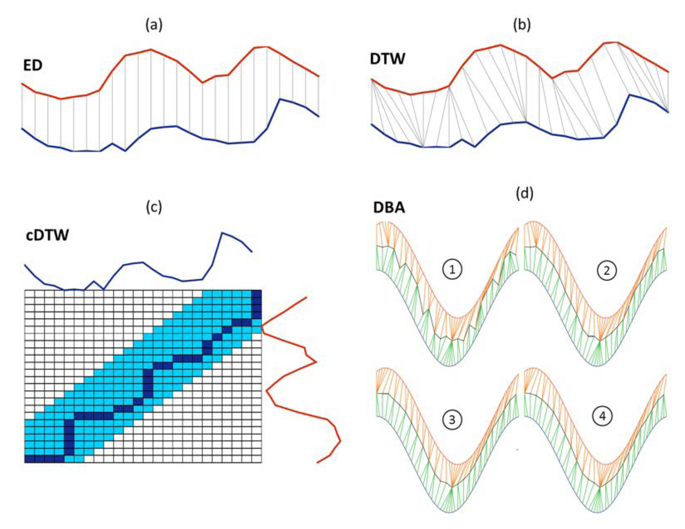
| Algorithm | Similarity Measurement | Centroid Computation |
|---|---|---|
| -means | ED [59] compares the two time series as follows: | The barycenter of potential cluster is calculated as follows [59]: The barycenter calculated discretely using ED as follows: |
| -DBA | DTW [54] compares as follows: where . is a nonnegative weighting coefficient to measure the goodness of warping function between points . | DBA [55] optimized the calculation of the barycenter for the application of DTW. As DTW takes the sequences association into consideration, the barycenter extraction conducted by using DTW is as follow: |
| -shape | SBD compares as follows [23]: where is the cross-correlation sequence with length . is computed as: | -shape optimizes the centroid extraction by finding the maximizer squared similarities to the other time trajectories [23]. The centroid is calculated iteratively as follows: |
| Year | Image Data (Julian) | RMSE (°C) | Standard Deviation (°C) | 2 × Standard Deviation (°C) | Correlation Coefficient |
|---|---|---|---|---|---|
| 2002 | 0704 (185) | 0.23 | 0.27 | 0.54 | 0.99 |
| 2005 | 0712 (193) | 0.23 | 0.21 | 0.42 | 0.98 |
| 2008 | 0820 (233) | 0.14 | 0.12 | 0.24 | 0.99 |
| 2011 | 0813 (225) | 0.23 | 0.26 | 0.52 | 0.97 |
| 2014 | 0728 (209) | 0.30 | 0.30 | 0.60 | 0.96 |
| 2017 | 0712 (193) | 0.20 | 0.22 | 0.45 | 0.99 |
| -Means | -cDBA | -Shape | |
|---|---|---|---|
| Accuracy | 0.6775 | 0.7725 | 0.6150 |
| RI | 0.9355 | 0.9387 | 0.9067 |
| ARI | 0.4680 | 0.4800 | 0.3896 |
| Purity | 0.6075 | 0.6475 | 0.5530 |
| Jaccard Score | 0.3355 | 0.3447 | 0.2423 |
| F-measure | 0.5735 | 0.6085 | 0.4623 |
| FM | 0.5025 | 0.5127 | 0.4523 |
| CSM | 0.5676 | 0.6174 | 0.5314 |
| NMI | 0.5991 | 0.6186 | 0.4808 |
| Entropy | 0.3865 | 0.3646 | 0.5058 |
| Cluster Number | Maximum | Minimum | Mean | Standard Deviation | ||||
|---|---|---|---|---|---|---|---|---|
| LLST | MSSI | LLST | MSSI | LLST | MSSI | LLST | MSSI | |
| 1 | 16.61 | −0.99 | 33.95 | 0.44 | 29.05 | −0.64 | 1.69 | 0.17 |
| 2 | 16.23 | −0.99 | 42.63 | 0.97 | 30.72 | −0.35 | 1.83 | 0.43 |
| 3 | 21.51 | −0.99 | 36.33 | 0.33 | 31.22 | −0.53 | 1.48 | 0.21 |
| 4 | 25.27 | −0.99 | 41.13 | 0.96 | 31.75 | −0.22 | 2.29 | 0.45 |
| 5 | 21.93 | −0.98 | 41.69 | 0.95 | 32.43 | −0.19 | 1.92 | 0.46 |
| 6 | 26.05 | −0.98 | 41.03 | 0.96 | 32.60 | 0.26 | 1.80 | 0.38 |
| 7 | 19.07 | −0.98 | 42.39 | 0.97 | 32.85 | 0.10 | 2.26 | 0.50 |
| 8 | 26.31 | −0.99 | 39.95 | 0.96 | 32.95 | −0.27 | 2.06 | 0.38 |
| 9 | 26.09 | −0.99 | 41.95 | 0.99 | 33.21 | 0.05 | 2.47 | 0.47 |
| 10 | 25.23 | −0.95 | 44.53 | 0.98 | 33.40 | 0.24 | 2.74 | 0.49 |
| 11 | 23.89 | −0.96 | 42.91 | 0.99 | 34.14 | 0.10 | 3.02 | 0.48 |
| 12 | 28.51 | −0.75 | 42.11 | 0.99 | 34.27 | 0.38 | 2.05 | 0.29 |
| 13 | 28.23 | −0.98 | 45.89 | 0.99 | 35.42 | 0.16 | 3.53 | 0.53 |
| 14 | 28.89 | −0.98 | 43.43 | 0.98 | 36.17 | −0.26 | 2.19 | 0.44 |
| 15 | 30.45 | −0.93 | 46.57 | 0.99 | 36.79 | 0.50 | 3.07 | 0.32 |
| 16 | 32.09 | −0.95 | 46.07 | 0.97 | 38.65 | 0.36 | 2.12 | 0.41 |
| 17 | 34.39 | −0.93 | 47.59 | 0.99 | 40.33 | 0.64 | 2.25 | 0.21 |
© 2018 by the authors. Licensee MDPI, Basel, Switzerland. This article is an open access article distributed under the terms and conditions of the Creative Commons Attribution (CC BY) license (http://creativecommons.org/licenses/by/4.0/).
Share and Cite
Liu, H.; Zhan, Q.; Yang, C.; Wang, J. Characterizing the Spatio-Temporal Pattern of Land Surface Temperature through Time Series Clustering: Based on the Latent Pattern and Morphology. Remote Sens. 2018, 10, 654. https://doi.org/10.3390/rs10040654
Liu H, Zhan Q, Yang C, Wang J. Characterizing the Spatio-Temporal Pattern of Land Surface Temperature through Time Series Clustering: Based on the Latent Pattern and Morphology. Remote Sensing. 2018; 10(4):654. https://doi.org/10.3390/rs10040654
Chicago/Turabian StyleLiu, Huimin, Qingming Zhan, Chen Yang, and Jiong Wang. 2018. "Characterizing the Spatio-Temporal Pattern of Land Surface Temperature through Time Series Clustering: Based on the Latent Pattern and Morphology" Remote Sensing 10, no. 4: 654. https://doi.org/10.3390/rs10040654