Measurements on the Absolute 2-D and 3-D Localization Accuracy of TerraSAR-X

Abstract

The German TerraSAR-X radar satellites TSX-1 and TDX-1 are well-regarded for their unprecedented geolocation accuracy. However, to access their full potential, Synthetic Aperture Radar (SAR)-based location measurements have to be carefully corrected for effects that are well-known in the area of geodesy but were previously often neglected in the area of SAR, such as wave propagation and Earth dynamics. Our measurements indicate that in this way, when SAR is handled as a geodetic measurement instrument, absolute localization accuracy at better than centimeter level with respect to a given geodetic reference frame is obtained in 2-D and, when using stereo SAR techniques, also in 3-D. The TerraSAR-X measurement results presented in this study are based on a network of three globally distributed geodetic observatories. Each is equipped with one or two trihedral corner reflectors with accurately (<5 mm) known reference coordinates, used as a reference for the verification of the SAR measured coordinates. Because these observatories are located in distant parts of the world, they give us evidence on the worldwide reproducibility of the obtained results. In this paper we report the achieved results of measurements performed over 6 1/2 years (from July 2011 to January 2018) and refer to some first new application areas for geodetic SAR.

1. Introduction

Space-borne SAR is mainly known for its ability to provide image observations of the Earth’s surface and the measurement of relative shifts making use of the carrier phase (i.e., SAR interferometry)—independent from weather and time of day. However, SAR offers several additional capabilities. The objective of this paper is to highlight the ability to provide also absolute localization accuracy of bright, well-detectable radar targets at centimeter level [1,2,3,4] with respect to a given geodetic reference frame like International Terrestrial Reference Frame, release 2014 (ITRF2014) [5]. Such a high accuracy—where TerraSAR-X/TanDEM-X lead worldwide among space borne SAR sensors [6]—can be achieved only if the SAR data are processed and calibrated with meticulous care and if they are corrected for well-known effects such as wave propagation and solid Earth dynamics, as it is done in geodesy [7].

Aiming at centimeter level accuracy, some basic aspects of SAR geolocation have to be reassessed. Therefore, the paper will start with a discussion of refinements compared to traditional techniques in the concept of SAR based location measurements. Furthermore, the verification of the localization accuracy requires a standard of comparison at least as good as SAR. Thus, we had to exercise utmost care with the installation and survey of our corner reflector (CR) test sites. If at least two SAR images with different acquisition geometries are involved, Stereo SAR techniques even allow to derive accurate 3-D on-ground coordinates when combining the ensemble of 2-D image coordinates. Equipped with this set of tools, we analyzed the geolocation accuracy of TerraSAR-X in detail, considering many potential influences like incidence angle, acquisition mode or polarization as well as the long-term stability of the SAR instrument or potential dependencies on the geographic location of the target. Our measurement results in 2-D and 3-D and their interpretation are the key aspects of this work. A brief outlook on an upcoming further improvement in geolocation accuracy and on some first applications for precise geolocation in the area of imaging geodesy, an area brought about by the geolocation capabilities of TerraSAR-X, completes the paper.

2. Background

2.1. Location Measurements by SAR

Radar systems indirectly measure geometric distances by means of the two-way travel time of radar pulses. The conversion from travel time to geometric distance, i.e., range, depends on the velocity of light (divided by two in order to convert from two-way travel time to one-way distance). Usually, the vacuum velocity of light is used in this context which however is larger than the true signal travel velocity if the signal passes through the Earth’s atmosphere. Here, electrons in the ionosphere as well as dry air and water vapor, mainly contained in the troposphere, introduce additional signal delays which have to be taken into account. The impact of the tropospheric delay on TerraSAR-X range measurements typically varies between 2.5 and 4 m depending on terrain height and incidence angle. The dispersive ionospheric delay at X-band for TerraSAR-X (9.65 GHz) amounts from several centimeters up to a few decimeters. The indirect annotation of the signal delays as part of the geometrical SAR range bias in units of length is common practice when generating SAR products, because it is convenient when correcting range measurements, but this leads to a mixing of different effects and complicates the usage of alternative atmospheric correction methods.

As atmospheric delays are likewise relevant for the Global Navigation Satellite System (GNSS) [8], which also applies centimeter wavelength radio signals (i.e., L-band, about 1‒2 GHz), the International GNSS Service (IGS) [9] provides path delay products inferred from the permanently operated GNSS receivers of the global IGS network. While the correction values for the non-dispersive (mainly tropospheric) delay can be directly applied to the SAR ranges, the correction values for the dispersive (mainly ionospheric) delay need to be adapted to the differences in the radio frequency (9.65 GHz instead of L-band) and the change in orbit height. Because the orbits of TerraSAR-X are significantly lower than the GNSS orbits and lie still within the upper ionosphere, only a portion of the entire Total Electron Content (TEC) in the ionosphere that is seen by GNSS has to be considered in TerraSAR-X datatakes. We found that the usage of a constant TEC scaling factor of 75% provides reasonable results [10].

Similar to the range, the azimuth coordinate of a ground target is indirectly given by a time measurement. As focused TerraSAR-X images correspond to zero-Doppler geometry, the azimuth position of the target in the image represents the time of closest approach between sensor and target. The conversion from azimuth time to a spatial coordinate is given by the zero-Doppler condition [11] and requires precise knowledge of the satellite’s orbit and the temporal synchronization between the orbit timeline and the operation of the radar instrument.

When assigning SAR measurements to a geodetic reference frame, the geodynamic effects shifting the true position of a ground target have to be considered in accordance with geodetic conventions [7]. The most prominent of these effects are solid Earth tides and plate tectonics which cause a periodic variation of up to a few decimeters over the course of a day or linearly accumulating shifts on the order of centimeters per year, respectively. The non-tidal atmospheric pressure loading (not part of the conventions) and the ocean tidal loading weigh on the tectonic plates and their variations shift the target position by up to several centimeters each. Pole tides occur due to the dynamics of the Earth’s rotational axis and are modeled as deviations with respect to a mean rotational pole. Their amount also varies at the millimeter level. Even weaker effects are caused by ocean pole tides and atmospheric tidal loading. Our correction values for the geodynamic effects applied to TerraSAR-X are based on the International Earth Rotation and Reference Systems Service (IERS) conventions, release 2010 [7]. However, plate tectonics are not covered by the IERS conventions as the geodetic techniques usually estimate them as part of the linear station coordinates, and therefore we have to consider them when modelling the target coordinates or reduce them in the SAR measurements.

In summary, the SAR measurements in range ${\tau }_m$ and azimuth $t_m$, corresponding to the zero-Doppler geometry of a CR, may be written as:

$$\begin{array}{c}{\tau }_m-\mathrm{\Delta }{\tau }_{cal}=\parallel {\mathit{X}}_s\left(t_{0D}\right)-\left({\mathit{X}}_t+\mathrm{\Delta }{\mathit{X}}_{geo}\right)\parallel ·2/c+\mathrm{\Delta }{\tau }_{tro}+\mathrm{\Delta }{\tau }_{ion}\\ t_m-\mathrm{\Delta }{t}_{cal}\iff \frac{{\dot{\mathit{X}}}_s\left(t_{0D}\right)·\left({\mathit{X}}_s\left(t_{0D}\right)-\left({\mathit{X}}_t+\mathrm{\Delta }{\mathit{X}}_{geo}\right)\right)}{\parallel {\dot{\mathit{X}}}_s\left(t_{0D}\right)\parallel ·\parallel {\mathit{X}}_s\left(t_{0D}\right)-\left({\mathit{X}}_t+\mathrm{\Delta }{\mathit{X}}_{geo}\right)\parallel }=0\end{array}$$

(1)

where ${\mathit{X}}_s$ and ${\dot{\mathit{X}}}_s$ are the satellite position and velocity vectors at the instant of closest approach $t_{0D}$, i.e., the zero-Doppler time which may be expressed in seconds of day UTC; the ${\mathit{X}}_t$ denotes the ITRF target coordinates that are corrected for the geodynamic effects $\mathrm{\Delta }{\mathit{X}}_{geo}$; the $c$ is the speed of light in vacuum, the $\mathrm{\Delta }{\tau }_{tro}$ and $\mathrm{\Delta }{\tau }_{ion}$ are the path delays of troposphere and ionosphere, and $\mathrm{\Delta }{\tau }_{cal}$ and $\mathrm{\Delta }{t}_{cal}$ refer to time biases, i.e., the geometrical calibration constants of the SAR sensor. Note that these equations are but an extension of the well-known range-Doppler equation describing the SAR observation geometry [11]. Both equations are coupled through the time dependency of the satellite state vector, and the azimuth is only implicitly defined by the geometric zero-Doppler condition; thus the $\iff$ has to be read as “corresponds to” and the $t_m-\mathrm{\Delta }{t}_{cal}$ should equal to the geometric $t_{0D}$. Note that strictly speaking, the azimuth also experiences secondary contributions from the atmospheric delays if there is a steep horizontal or temporal gradient in the atmospheric portion traversed by the two-way signal, which is transmitted and received by the radar at separate times at separate locations. The typical integration time of a single target, however, is in order of some seconds; hence we do not consider this in our azimuth measurements.

2.2. SAR Positioning with Stereo SAR

Measuring the position of a target in a radar image determines only its 2-D location in the slant range and azimuth geometry defined by the 3-D to 2-D projection of the SAR imaging process. In order to determine the target’s underlying 3-D location, at least two images with sufficient angular separation have to be used, which enable a stereo setup and ultimately the retrieval of the CR coordinates. Expanding this concept to a more general method by employing least-squares parameter estimation, any number of radar images larger than one may be combined in a consistent estimation of the target position. This general approach is the core of our Stereo SAR method which is extensively discussed in [12]. In the following, we provide only a short summary and the reader interested in more details is referred to the paper. By using the range-Doppler equations (Equation (1)) as two condition equations that couple the measurements ${\tau }_m,t_m$ with the target position ${\mathit{X}}_t$, one can solve for the coordinates by performing a rigorous linearization and employing an iterative computation scheme. The theory behind this method may be found in [13]. In accordance with Equation (1) the condition equations read:

$$\begin{gathered} \parallel {\mathit{X}}_s\left(t_m^{*}\right)-{\mathit{X}}_t\parallel - {\tau }_m^{*}=0 \\ \frac{{\dot{\mathit{X}}}_s\left(t_m^{*}\right)·\left({\mathit{X}}_s\left(t_m^{*}\right)-{\mathit{X}}_t\right)}{\parallel {\dot{\mathit{X}}}_s\left(t_m^{*}\right)\parallel ·\parallel {\mathit{X}}_s\left(t_m^{*}\right)-{\mathit{X}}_t\parallel }=0. \end{gathered}$$

(2)

The ${\tau }_m^{*}$ and ${\tau }_m^{*}$ are the refined measurements already corrected for the atmospheric path delay and with the geometrical calibration applied. The least-squares method resolves the remaining inconsistencies of the equations by estimating observation residuals, which are minimized according to the L2-norm, and it estimates the optimal target coordinates at the same time. Be aware that the satellite orbit ${\mathit{X}}_s$ and ${\dot{\mathit{X}}}_s$ is provided with the SAR image annotation and it is kept fixed in the processing. The orbit is modelled through short arc polynomials [12], but the along-track relationship of the azimuth observation with the orbital state vector is fully maintained through the linearization. We do not introduce any a priori variance information for the individual measurements, but variance component estimation [14] is part of the solution process to infer a common variance for all the range measurements and a common variance for all the azimuth measurements. This ensures optimal weighting between the two types of SAR measurements.

The outcomes are not only the position coordinates but also the estimation of the positioning accuracy, i.e., the variance-covariance (VC) matrix of the coordinates stemming from the solution of the mathematically overdetermined problem. The VC matrix characterizes the geometry of the underlying stereo setup and the quality of the SAR measurements inferred from the minimized residuals; hence it also enables a reliable characterization of the coordinate solution. It is a fully populated 3 by 3 matrix with the main diagonal holding the variances ${\sigma }_{xx}^2$, ${\sigma }_{yy}^2$ and ${\sigma }_{zz}^2$ referring to the global frame, but the VC matrix may be transformed to express the estimated accuracy for any frame orientation, for instance the local north, east and height frame. A useful way of visualizing the VC matrix is the error ellipsoid, which is the decomposition of the matrix for its eigenvalues [13,15]. However, the confidence level of the VC matrix of 3-D coordinates as computed by the least-squares method is only about 20% [13]; hence for our positioning results we scale all the variance-covariance estimates to a more reliable confidence level of 95% by applying the corresponding scaling factor of the F-distribution [15], which is typically in the order of 2.85 because of the large number of TerraSAR-X images available for our analysis.

3. Materials and Methods

3.1. Verification of the Geolocation Accuracy of SAR

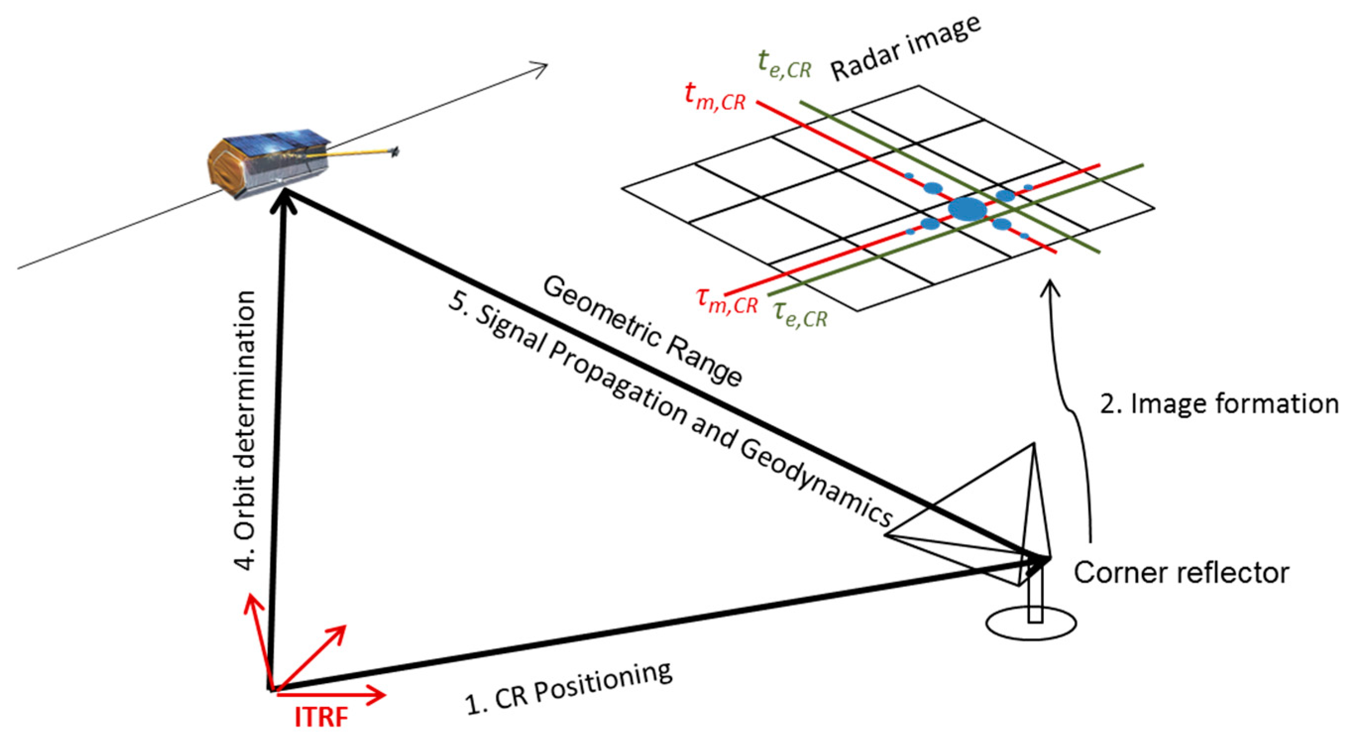
A widely used approach to verify the geolocation accuracy of SAR is based on artificial point-like targets deployed on ground [16]. Their positions in focused SAR images are measured and compared to the expected values that are derived from the knowledge of the target’s on-ground coordinates and the determination of the satellite position at closest approach. The conversion from spatial coordinates to expected radar time coordinates is based on the zero-Doppler equations (Equation (1)) and the interpolation of the satellite’s orbit, i.e., the reverse approach to the location measurements of SAR, discussed in Section 2.1.

Due to the well-defined shape of their impulse-response and to their high radar cross section (RCS), the exact positions such artificial targets in SAR images are precisely detectable so that the location accuracy mainly depends on the geometric features of the object of research: the end to end SAR system consisting of SAR sensor and SAR processing system. In contrast for weaker “natural” targets, their detectability in the surrounding clutter is the limiting factor for the location accuracy so that such targets give little incidence on the geometric accuracy of the end to end SAR system. Following [17], which includes a modified form of earlier work by Stein [18] and Swerling [19], the effect of the clutter on the obtainable localization accuracy is given by:

$$\sigma =\frac{\sqrt{3}}{\pi \sqrt{2}}·\frac{\rho }{\sqrt{SCR}}\approx 0.39·\frac{\rho }{\sqrt{SCR}}$$

(3)

where $\sigma$ denotes the expected clutter contribution to the standard deviation of the target location, and $\rho$ is the resolution of the target in terms of the 3 dB width of its impulse response. Different from [17], an additional factor $\sqrt{1/2}$ is introduced here, considering that we examine the localization accuracy of a single SAR measurement, whereas [17] refers to the mutual distance of two SAR measurements.

The most common types of point-like targets are passive corner reflectors (CRs) and active radar transponders. Appreciated features of purely passive elements like CRs are that they neither need any power-supply nor do they introduce any (possibly unknown) additional delays to the signal round trip time. Moreover, the electric phase center position is equal to the inner corner position which can be determined readily. The intersection of the three orthogonal plates is a well-defined point, for which the ITRF2014 coordinates may be accurately determined by terrestrial geodetic survey.

While the verification approach sketched in Figure 1 looks simple on the first glance, its realization requires meticulous care during all processing steps when centimeter or even millimeter accuracy is aspired (In [20], Small et al. give a detailed guideline on the installation of a CR test site). The CRs have to be firmly installed (preferably on stable bedrock or second-best on a firm concrete foundation) and correctly aligned. Their reference coordinates have to be very accurately determined. If possible, the deployment at well-known geodetic reference sites is advised when verifying the SAR geolocation capability. As any motion or re-orientation operation is prone to introduce spurious errors, we advise against any actions that could invalidate the geodetic reference coordinates of the phase center. Instead the reflectors should be kept fixed and their coordinates verified every 1‒2 years.

Once the CRs are installed and SAR datatakes are acquired, the target positions in the focused images have to be measured with sub-pixel resolution using oversampling and interpolation techniques, and the extracted radar times have to be corrected for the estimated propagation delays and geodynamic effects (as detailed in [21]). We recommend to use Single-look Slant-range Complex (SSC) image products for geolocation measurements instead of ground-projected image products (i.e., TerraSAR-X product types MGD, GEC and EEC), as any ground-projection introduces an avoidable additional error source.

By performing many verification measurements at several test sites far apart from each other, and employing SAR images acquired in different SAR modes, at different times, as well as varying the site position within an image and the overall imaging conditions (e.g., features like polarization, incidence angle or orbit direction: ascending or descending), the SAR imaging system can be very accurately geometrically calibrated and verified. Moreover, error estimates can be given and residual systematic biases can be characterized. Regular observations over long time spans (years) enable investigations of seasonal effects and the long-term stability of the measurement results.

3.2. Geometric Recalibration of the Sensor

The operational TerraSAR-X products are already prepared for the consideration of atmospheric effects [22] and their product annotation contains estimates for tropospheric and ionospheric signal propagation delays. These delay values are composed of scene-dependent tropospheric and ionospheric delays derived from a simplified static height-dependent model [23], and a set of associated system calibration constants determined during the mission’s initial calibration campaigns. With these annotated parameters systematic biases in the measured target positions are avoided and geolocation accuracy at decimeter level can be achieved [22], which is already beyond the product specification of 1 m [24].

However, these calibration constants need to be refined when we change the measurement concept and correct the SAR geolocation measurements for signal propagation with the more precisely measured atmospheric delay values provided by the IGS, and also take the geodynamic effects into account. Because of different biases of the atmospheric and geodynamic models involved, an adapted set of constants was necessary and we had to determine recalibration constants for both TerraSAR-X satellites, TSX-1 and TDX-1, to match this refined measurement concept. Note that, using our refined geodetic concept, TerraSAR-X is now fully compatible with the well-established standards of the GNSS community. Because the image user has no influence on the operational SAR focusing process, the only manageable way to apply our recalibration constants is that the user explicitly modifies his measured azimuth and range times by them.

The recalibration constants result from the median location offsets in azimuth and range obtained at reference test site(s). We use the median instead of the mean value because it is less sensitive to outliers, as the presence of a few of them is hardly avoidable in long measurement series.

Because most of our datatakes are in the HH polarization, we started to recalibrate this polarization channel first. After that, the calibration of the VV channel is efficiently performed on the base of dual-pol (HH/VV) datatakes. Here, both polarization channels are imaged at the same time, so that almost all influencing factors (like the exact amount of atmospheric delays and solid Earth dynamics, the exact satellite orbit and the exact CR position) are equal in both channels and consequently cancel out in a relative measurement of the target position offset performed in both channels. In consequence, also error contributions from the limited knowledge of these influences cancel out and we needed significantly less dual-pol datatakes to determine only the difference between the calibration constants of both channels. In comparison, the amount of single-pol datatakes required in an independent calibration of the VV channel with comparable accuracy was much larger.

3.3. Our TerraSAR-X Test Sites

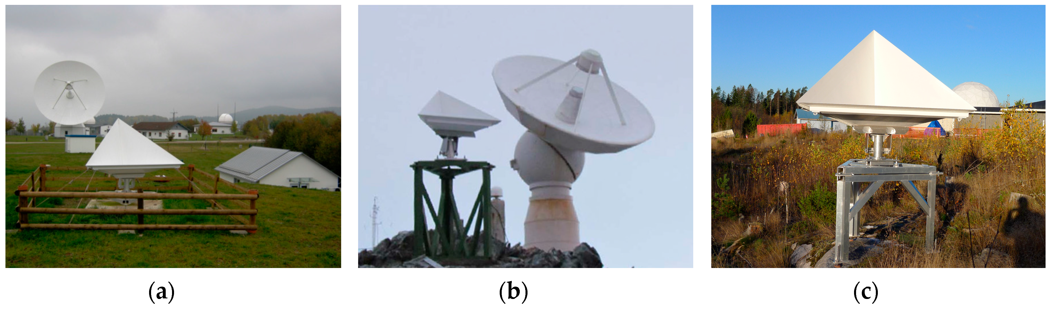
The network of our test sites [3] grew step by step over the course of our investigations. In the final state, three test sites with in total five trihedral CRs are involved in our measurement series. The geographic distribution of these test sites spans from Germany and Finland to the Antarctic Peninsula (see Figure 2a‒c). All of our CRs are mounted close to a local IGS reference station. Benefitting from this vicinity, the ground positions of the reflectors are known very precisely (< 5 mm) relative to the station reference coordinates from terrestrial geodetic survey. The particulars of the individual TerraSAR-X measurement series and the incidence angles of the datatakes involved are summarized in

Table 1. Key figures of our SAR measurement series at geodetic observatories. Each CR is seen from two or three adjacent orbits though the CR is optimally oriented for only one of them (see column “optimum incidence angle”).

Corner Reflector/ Measurement Series	Acquisitions Started at	Optimum Incidence Angle 1	Additional Incidence Angle(s)
Wettzell Ascending	12 Jul. 2011	34°	46° (since 2 Mar. 2013)
Wettzell Descending	11 Dec. 2013	45°	33°, 54°
GARS O’Higgins Ascending	27 Mar. 2013	38°	30°, 45°
GARS O’Higgins Descending	24 Mar. 2013	35°	42°
Metsähovi Descending	4 Nov. 2013	37°	27°, 46°

¹ w.r.t. the orientation of the CR.

.

In July 2011, we installed our first 1.5 m CR at the Geodetic Observatory Wettzell, Germany (Figure 2a). It is firmly mounted on a concrete foundation and horizontally oriented for acquisitions from ascending orbits and vertically aligned for an incidence angle of 34 degrees. In order to investigate possible angular dependencies in the position offsets measured with TerraSAR-X, we set up a second, parallel acquisition series of this CR using datatakes from an adjacent ascending orbit with a 46 degrees incidence angle. In order to preserve the precisely measured geodetic reference coordinates of the CR, we left its orientation unchanged and accepted the slight reduction in the RCS by about 2 dB. This fixed installation method was also adopted for the other subsequently installed reflectors, which are aligned for either ascending or descending passes, and their vertical orientation was adjusted for the center of the radar beam used at the site, see column “optimum incidence angle” in Table 1.

In December 2013, we installed a second 1.5 m CR at Wettzell. Oriented for descending orbits and regularly imaged with different incidence angles (45 degrees, which is optimum w.r.t. the CR orientation, and additionally 33 and 54 degrees) from three adjacent orbits, it enlarges the number of acquisition geometries at this test site.

Since March 2013, there are two 0.7 m CRs at our second test site, close to the German receiving and research station GARS O’Higgins located at the Antarctic Peninsula (Figure 2b). One of the CRs is oriented for ascending, the other for descending orbit passes. Because of the demanding local weather conditions, each CR is mounted above the usually experienced winter snow level using an additional 1 m base frame (see Figure 2b), and both are covered by a high-frequency transparent Gore-Tex™ (Gore-Tex is a trademark of W.L. Gore & Associates, Newark, DE, USA) canvas. The latter significantly eases the local maintenance due to snow. The CRs are still not maintenance-free, but the canvas avoids snow and ice within the reflector where they are more difficult and more cumbersome to remove than at the covering canvas.

Finally, there is our third test site at the geodetic observatory in Metsähovi, Finland, where one 1.5 m CR oriented for descending orbits was installed in October 2013 (Figure 2c). Similar to GARS O’Higgins, the CR is mounted above the expected snow level on a 1 m frame base. Benefiting from local ground conditions, the frame base is anchored by rods and rock epoxy glue residing in deep holes drilled into stable bedrock.

3.4. TerraSAR-X Datatakes

As of 1 February 2018, both TerraSAR-X sensors—TSX-1 and TDX-1—acquired in total 1060 datatakes for our test sites. The datatake acquisition is still ongoing in order to evaluate possible long-term trends. High resolution imaging modes are preferable when aiming for centimeter or millimeter measurement accuracy level with SAR, because the mode directly affects the image resolution and the signal to clutter ratio (SCR) and thus the extraction accuracy of the range and azimuth coordinates from the SAR image [17,18,19]. Consequently, we opted for HS300 mode, i.e., the high resolution sliding spotlight mode with an average slant range and azimuth resolution of 0.6 m by 1.1 m [24], for the majority of our TerraSAR-X acquisitions, because the even better Staring Spotlight mode ST300 was not available at the time when our measurement series started. Thus, only a few ST300 datatakes are included in our acquisition series. Almost all of our datatakes are in HH polarization. The only exception is a recently started HS dual-pol (HH/VV) measurement campaign at Wettzell where we investigate polarization channel dependent offsets. In order to avoid saturation of our 1.5 m CRs in the focused SAR images, the L1B products of the datatakes were ordered to be processed with gain attenuation (10 dB for HS300 and even 20 dB for ST300). The nominal backscatter values for our CRs are 30.2 dBm² for the 0.7 m and 43.4 dBm² for the 1.5 m reflectors.

TerraSAR-X datatakes are subject to DLR’s copyright and to security regulations of German law, which prohibit any unauthorized redistribution. Thus, we have to refer scientists interested in reproducing our measurement results to the EOWEB catalogue [25], where TerraSAR-X L1B products can be ordered by registered users (scientific proposal submission under [26]). The image center coordinates, required to select datatakes of our test sites from catalogue, are listed in

Table 2. Image center coordinates of the datatakes underlying our measurements.

Test Site	Latitude [°N]	Longitude [°E]
Wettzell	+49.145	+12.876
GARS O’Higgins	‒63.321	‒57.902
Metsähovi	+60.217	+24.395

.

4. Results and Analysis

4.1. Monitoring the Operational Readiness of a CR

A lesson learned from our long-term measurement series, is to be aware of weather influences affecting the performance of a CR [21]. Snow within the CR changes the backscatter geometry and in consequence firstly lowers the CR’s RCS and secondly—much more problematic for our measurements—it changes the actual position of the CR phase center. Because the CR models we installed have drainage holes at their converging corners, rain is in general not a problem, except when leaves fallen or blown into the CR may clog the drainage hole.

As the significantly lowered RCS is a good indicator for such disturbances, we routinely monitor the RCS and compare its value against the expected value derived from theory or experience. Based on an empirically derived threshold of 3 dB RCS loss relative to the expected value, we are able to identify the TerraSAR-X measurements affected by such irregular conditions and exclude them from further analyses, where they would otherwise occur as coarse (i.e., decimeter-level) outliers. During our analysis we did not observe any significant correlation of moderate RCS losses of less than 3 dB with the shifts in the SAR measured CR locations.

Over the course of our investigations and based on this assumption, we identified in total 79 disturbed location measurements, reducing the number of datatakes in the analysis from 1060 to 981. In contrast, there still remain 18 measurements (approximately 1.8%) with a conspicuously high location error of 7‒11 cm where no obvious external cause could be identified. With the exception of one, these values are found in azimuth. Because we have no indication for an external cause, these measurements must not be excluded from analysis.

4.2. Geometric Recalibration Constants

We have chosen the CR at the Metsähovi test site as the reference for our TerraSAR-X recalibration. Here, the mounting of the CR on stable bedrock provides confidence that the geodetic coordinates of its phase center are even more long-term stable than the ones from our other test sites. Because the measurement series are in HH polarization mode, we originally focused our recalibration activities on this mode and just recently complemented them by deriving recalibration constants for VV polarization too.

Table 3. Applied geometric calibration constants in seconds and converted to spatial distances.

Satellite	Polarization	Azimuth [s] 1	Range [s]	Azimuth [m] ²	Range [m] ³
TSX-1	HH	‒9.7·10‒6	‒2.01·10‒9	‒0.068	‒0.301
TSX-1	VV	‒9.7·10‒6	‒2.28·10‒9	‒0.068	‒0.342
TDX-1	HH	‒7.7·10‒6	‒1.82·10‒9	‒0.054	‒0.273
TDX-1	VV	‒7.7·10‒6	‒2.09·10‒9	‒0.054	‒0.313

¹ For comparison purposes: The operational calibration constant w.r.t. azimuth amounts to ‒11.2·10^‒6 s for TSX-1 and ‒6.8·10^‒6 s for TDX-1. ² Converted with average TerraSAR-X ground track velocity of 7050 m/s. ³ Converted with speed of light in vacuum and divided by 2 for one-way.

shows our new calibration constants to be applied by the user. To remain consistent with the sign convention of the operational calibration constants, our recalibration constants have to be subtracted from the measured radar times at all test sites (i.e., the absolute value of the negative constants has to be added!). For convenience, Table 3 also shows the values converted to distances. Note that we use an average ground track velocity as conversion factor for azimuth here, whereas the precise value in a given SAR image depends on geometric factors like the incidence angle and the topographic height.

In addition to the operational range calibration constant that is already implicitly applied during TerraSAR-X image focusing, we had to introduce a range recalibration constant that the user has to apply explicitly. The amount of our range recalibration constant corresponds to about 30 cm spatial distance, see Table 3. The cause for its necessity can be found mainly in the different handling of the wet part of the tropospheric delay in both measurement concepts. Being the most volatile contribution to the tropospheric delay, its consideration is beyond the capabilities of the simplified model underlying the annotated delay value and in consequence, it contributes in average to the operational calibration constant. When we make use of the measured tropospheric delay of the IGS, the wet delay is already included and must not be considered twice. Thus, our recalibration constant figures as a readjustment of the wet delay’s contribution in the operationally applied calibration constant.

The likely explanation for the small difference of 0.27 nanoseconds (equivalent to 4 cm) discovered in the range calibration constants of both polarization channels (cf. Table 3) might be found in the staggered mounting of H and V antenna elements on the satellite’s surface and in the slightly different signal routing inside the sensor electronics.

In contrast to the range, the operational calibration constant in azimuth is not applied in the processor; hence a user is able to replace it with our new constants. The differences between the results of the operational calibration and our recalibration are rather small (corresponding to about 11 mm spatial distance for TSX-1 and 6 mm for TDX-1). However, we benefit from the long duration of our measurement series, the more precisely determinable CR reference coordinates in the vicinity to the IGS reference stations, and from the firm orientation of the CRs that avoids any undesirable change of their phase centers. Due to these factors, we were able to slightly refine the azimuth calibration constants of both sensors.

Finally, we want to give some remarks on the cross-polar channels. Because trihedral CRs do not change the plane of polarization, our CRs are invisible in cross-polar image channels, as they are employed in polarimetry. Consequently, a geometric recalibration of the cross-polar channels HV and VH is out of the capabilities of our on-ground measurement equipment, but we can provide assumptions about adequate recalibration constants for the cross-pol channels based on theoretical considerations. Assuming that most of the differences between the examined co-polar channels HH and VV results from construction particulars of the antenna and the sensor electronics, we might conclude that the recalibration constants for HV and VH are approximately in the mean of the HH and VV constants, because HV shares the transmit path with the HH channel and the receive path with the VV channel, while the opposite is true for VH.

4.3. Temporal Stability of SAR Geolocation Results

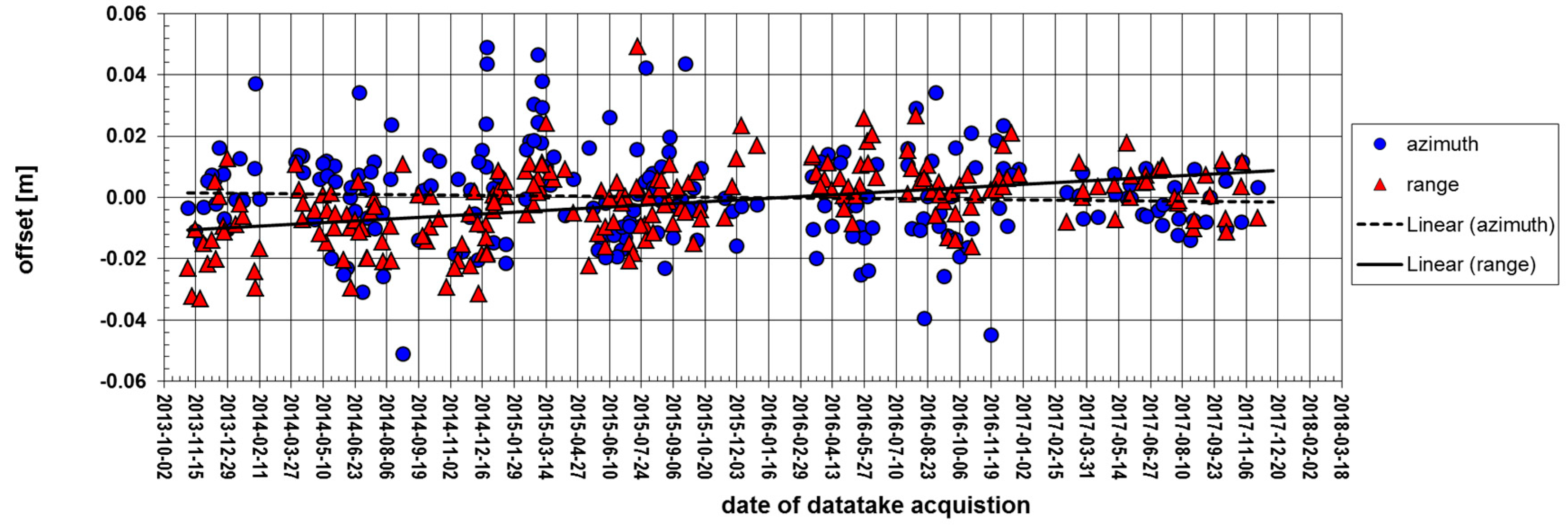
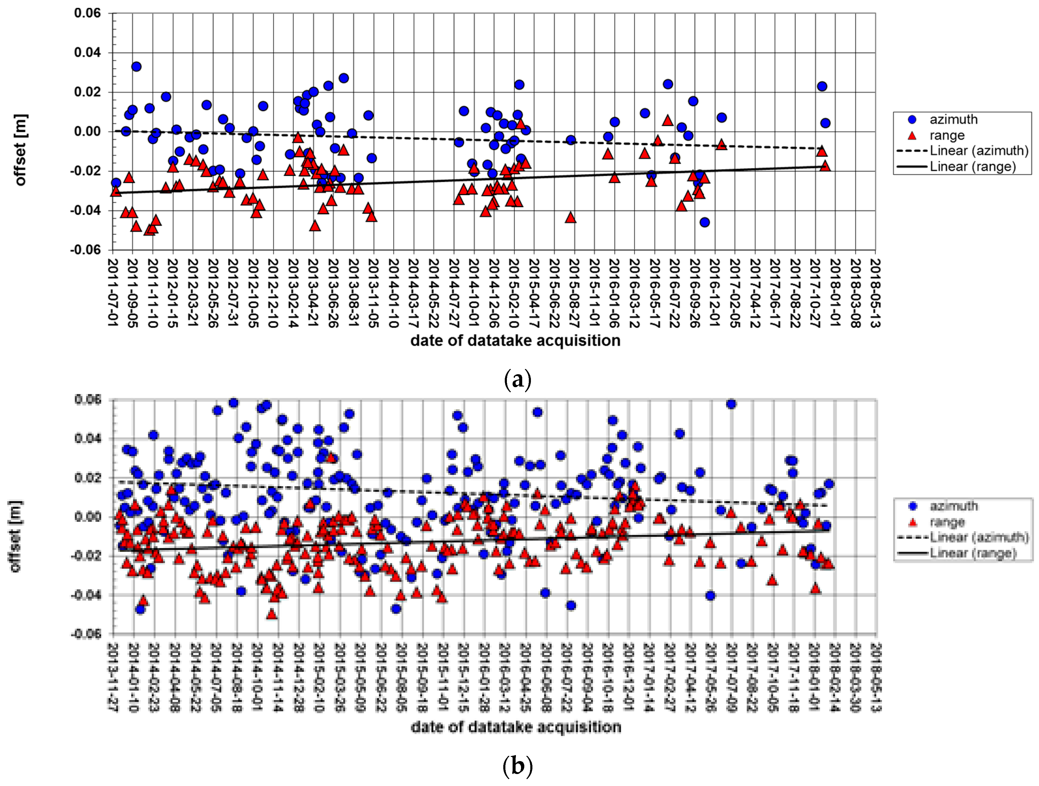
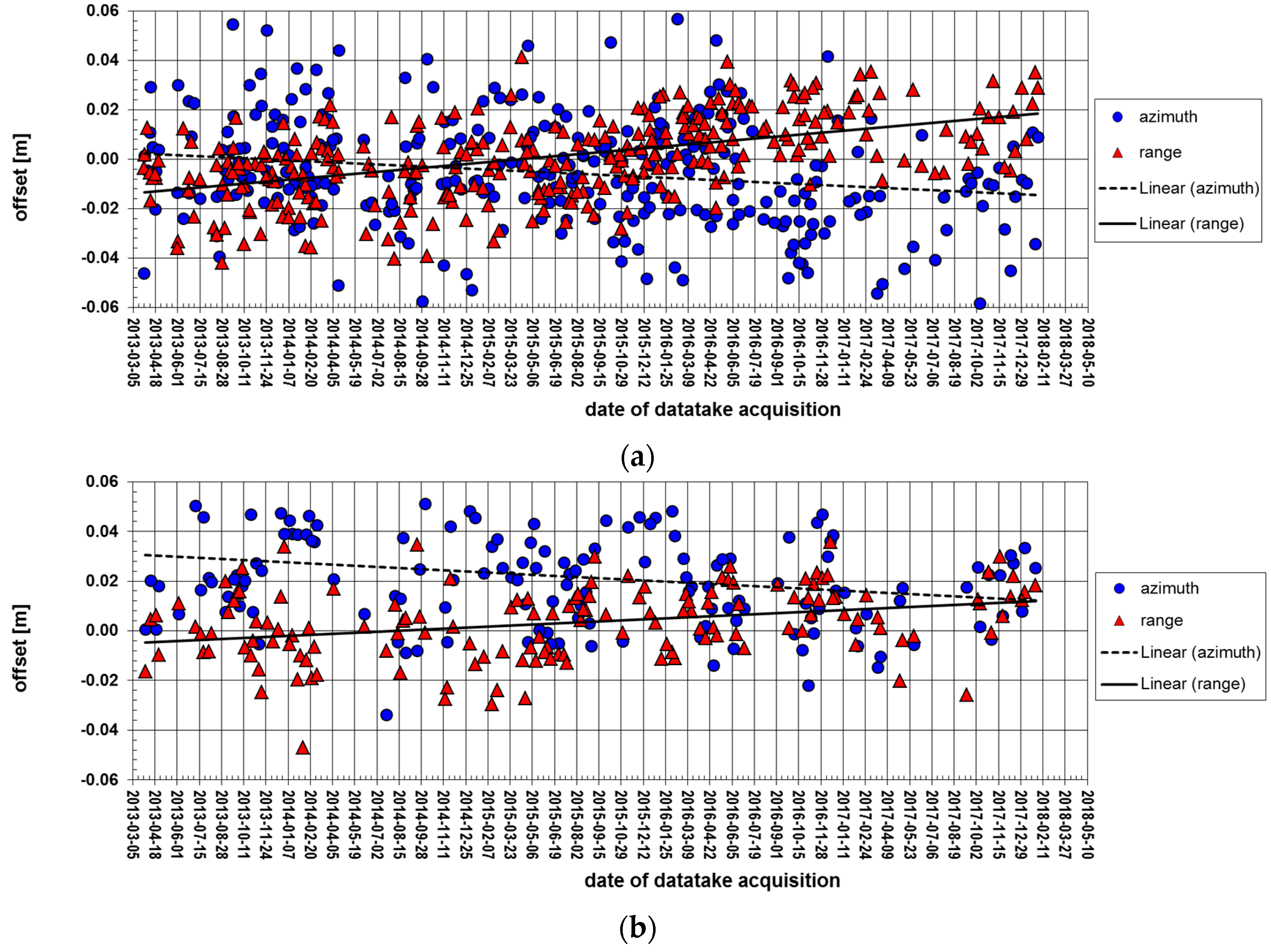
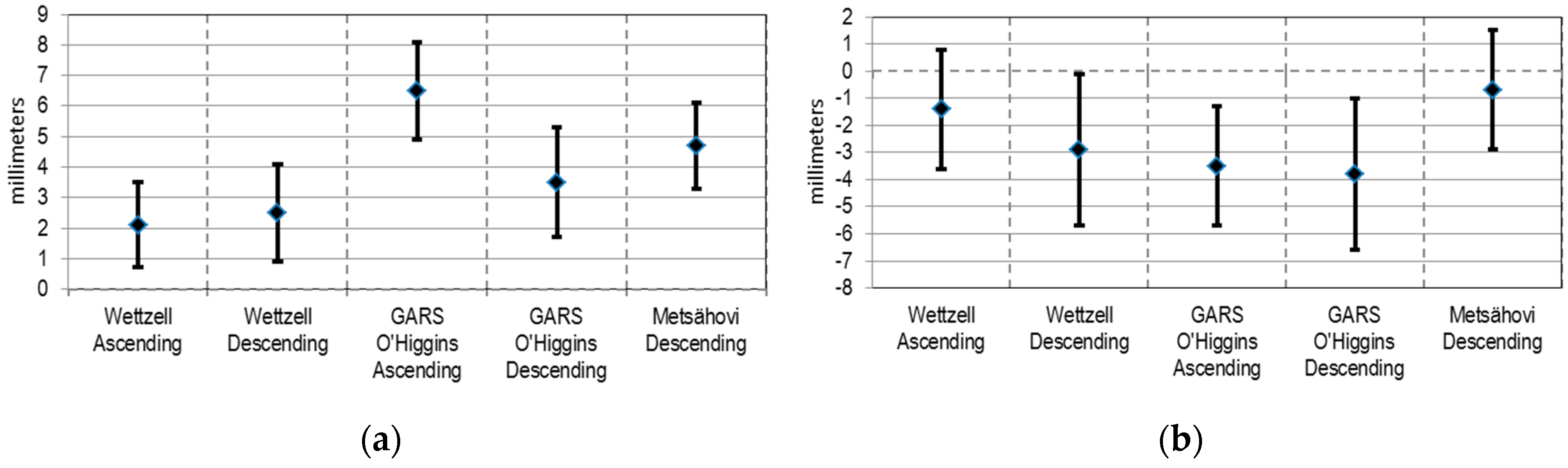
Figure 3, Figure 4 and Figure 5 show the temporal progression of the azimuth and range offsets between measured and expected radar coordinates at our three test sites. A slight trend is perceivable from all plots. In all measurement series, there is a tendency of the measured values toward early azimuth and toward far range. In order to estimate the magnitude of this trend, we approximated the temporal progressions of the offsets by a linear function and investigated the obtained gradients.

Table 4. Interpolated linear trend of the observed offsets: Mean value and standard deviation (1σ) of the gradient.

Measurement Series	Azimuth Gradient [mm/y]	Range Gradient [mm/y]
Wettzell Ascending	‒1.4 ± 1.1	+2.1 ± 0.7
Wettzell Descending	‒2.9 ± 1.4	+2.5 ± 0.8
GARS O’Higgins Ascending	‒3.5 ± 1.1	+6.5 ± 0.8
GARS O’Higgins Descending	‒3.8 ± 1.4	+3.5 ± 0.9
Metsähovi Descending	‒0.7 ± 1.1	+4.7 ± 0.7

and Figure 6 show that the gradients are in the order of millimeters per year and exceed the standard deviation (1σ) expected from error propagation. However, the 1σ just represents a 68% confidence interval whereas for a 95% confidence interval 2σ is required [15]. The gradients in range even exceed 3σ so that a confidence level of more than 99.7% results. Therefore we consider the range effect to be significant. For the azimuth, the results from the different test sites are much less distinct and some of the estimated gradients (Wettzell Ascending and Metsähovi Descending) obviously remain below the 2σ, thus the continuation of the ongoing measurement series is required to reduce the remaining uncertainty.

Assuming that the trend in the range measurements is real, finding a possible cause for it is subject of ongoing investigations. We may already excluded some potential causes: The stability of the sensor internal clock rate governing all timings in the SAR payload is routinely monitored in the TerraSAR-X mission and in this way known with nine digit accuracy (the technique is described in [27]). In consequence, this error contribution cannot exceed 3 mm and is therefore below the amount of the observed trends. Also the satellite orbit determination is not considered to be a cause because we have independent measurements of the TerraSAR-X orbits based on Satellite Laser Ranging (SLR) confirming the long-term stability—see [28] for more. Thus, the focus of our further investigations has to be on the SAR sensor itself. We might investigate e.g., whether slight aging effects in electronic components are supposable. The challenge is that to our knowledge no prior space-borne SAR sensor was examined after insert to orbit at a comparable level of detail.

4.4. Analysis for Angular Dependencies

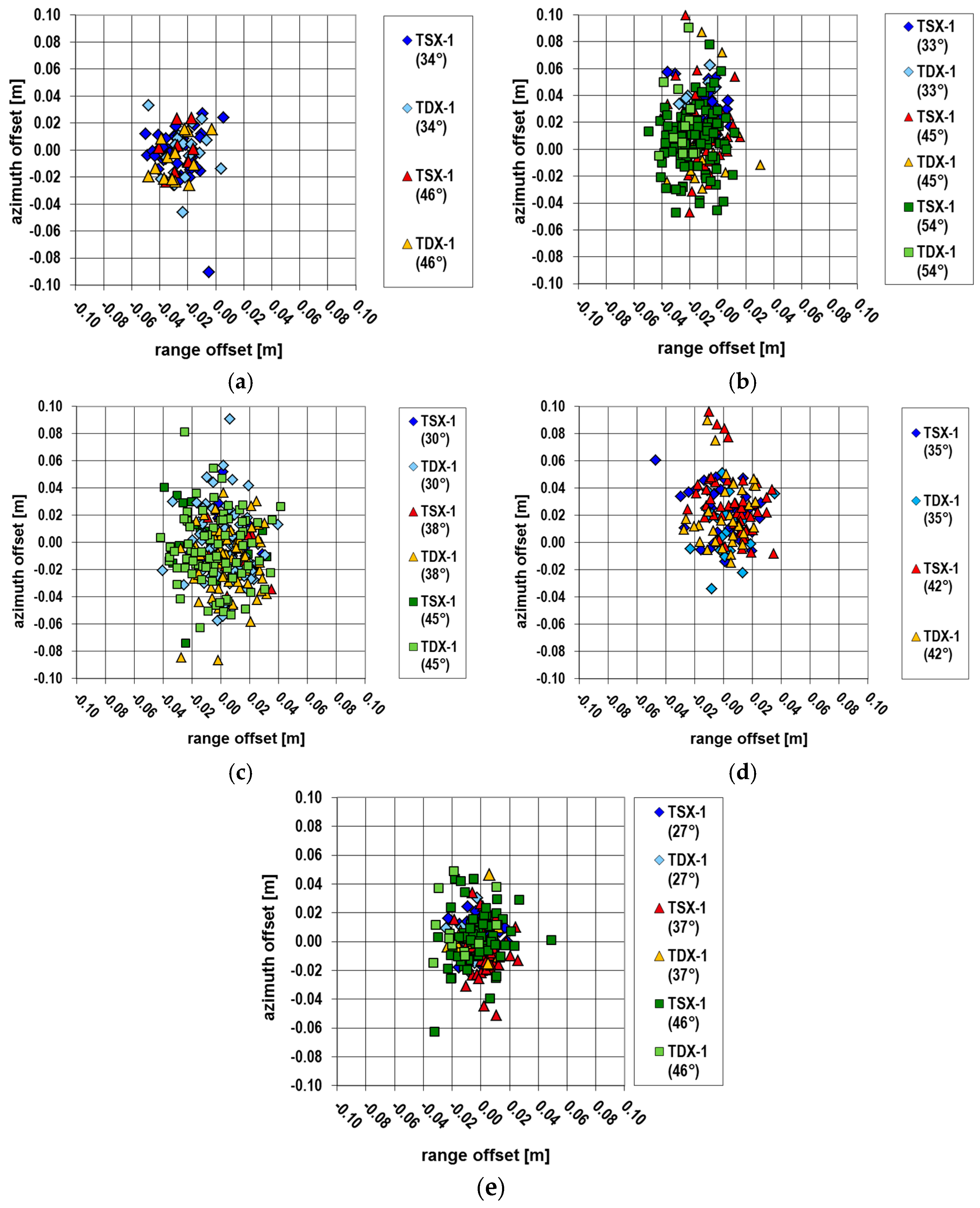
Figure 7a‒e show the scatter plots of the azimuth and range offset obtained between measured and expected radar coordinates for the different measurement series. In each plot, different colors represent acquisitions from different incidence angles.

By visual inspection, the single distributions coincide for the different incidence angles and no significant dependency between incidence angle and location offset is perceivable. In order to quantitatively verify this hypothesis, we performed a statistical analysis of the location offsets. The resulting mean values and standard deviations are listed in

Table 5. Incidence angle wise mean values and standard deviations (1σ) of the obtained range and azimuth error.

Measurement Series	Incid. Angle	# of Meas.	Azimuth Offset [mm]	Range Offset [mm]
Wettzell Ascending	34	65	‒2.9 ± 18.6	‒25.1 ± 12.0
	46	23	‒4.1 ± 15.5	‒27.4 ± 10.5
Wettzell Descending	33	42	+29.5 ± 15.7	‒10.4 ± 11.2
	45	75	+11.5 ± 25.3	‒8.3 ± 13.2
	54	112	+8.0 ± 23.7	‒17.2 ± 13.1
GARS O’Higgins Asc.	30	112	‒0.7 ± 23.5	+3.9 ± 17.0
	38	86	‒11.6 ± 22.9	+5.0 ± 14.8
	45	104	‒5.3 ± 25.7	‒5.2 ± 18.8
GARS O’Higgins Desc.	35	62	+17.6 ± 19.8	+0.9 ± 14.9
	42	85	+24.9 ± 23.2	+4.9 ± 14.0
Metsähovi Descending	27	61	+3.5 ± 10.7	‒2.5 ± 9.3
	37	75	-4.0 ± 15.6	+1.2 ± 9.7
	46	79	+1.6 ± 22.3	‒4.4 ± 15.0

, sorted by incidence angle. The variations across the mean values of one site are usually lower than the standard deviation of the single measurement series, and no particular systematic dependency on the incidence angle can be found. We conclude from these results that the individual beams are consistent.

4.5. Comparison of Different Imaging Modes

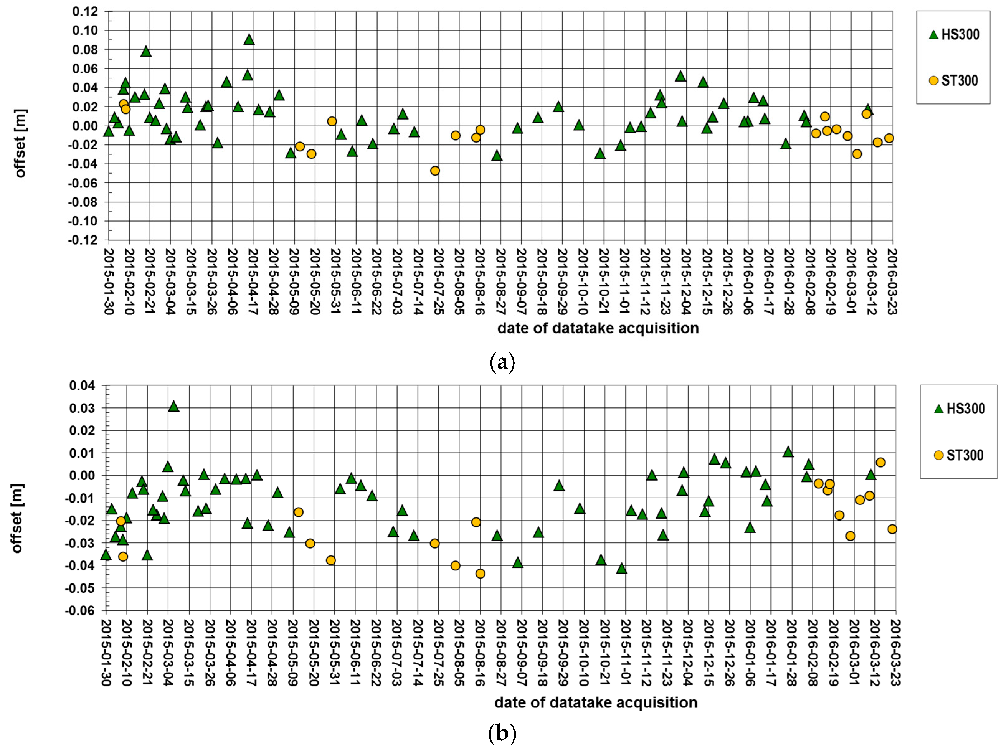
Figure 8 shows the temporal progression of the azimuth and the range offset at the Wettzell test site during the Staring Spotlight (ST300) campaign from February 2015 until March 2016.

The Staring Spotlight datatakes interleave the series of regular Sliding Spotlight (HS300) acquisitions. The plots indicate the consistency of the location results from both imaging modes as the short term patterns in the azimuth and range offsets progress across the varying imaging modes.

4.6. Location Independency of Results

Table 6. CR wise mean values and deviations (1σ) of the obtained range and azimuth error.

Measurement Series	# of Measurements	Azimuth Offset [mm]	Range Offset [mm]
Wettzell Ascending	88	‒3.2 ± 17.7	‒25.7 ± 11.6
Wettzell Descending	229	+13.1 ± 24.3	‒13.0 ± 13.4
GARS O’Higgins Ascending	302	‒5.4 ± 24.4	+1.1 ± 17.6
GARS O’Higgins Descending	147	+21.8 ± 22.1	+3.2 ± 14.5
Metsähovi Descending 1	215	+0.2 ± 17.5	‒1.9 ± 12.0

¹ The reason, why the average position offset in this measurement series is almost zero, is that we used the Metsähovi CR as calibration reference for all of our test sites, see Section 4.2.

shows the overall mean values and standard deviations of the localization error determined at our different test sites. As Metsähovi is used as our recalibration reference, the mean location offset is consequently close to zero and does not contain any useful information. However, the standard deviation determined at this test site is not influenced by the recalibration and therefore it is still an independent measurement result.

The obtained mean values at the other test sites indicate the consistency between SAR location measurements and the calibration derived for Metsähovi. They amount from few millimeters up to 2.6 cm. The maximum range bias results for the Wettzell Ascending CR. However, a terrestrial resurvey of this reflector disclosed the cause for the deviating behavior of this single measurement series: The concrete foundation of the CR subsided by about 2 cm during the first 2 years after the CR was installed and surveyed. While we chose the location for our first CR with regard to a minimum disturbance in the radar image from the installations of the IGS reference station, we did not take enough care of the ground conditions and put the foundation on a small mound rising above the local surroundings, see Figure 2a. As lesson learned, we more carefully considered this aspect when installing the other CRs.

The standard deviations of the single measurement series in range vary from 12 to 18 mm. The standard deviation in azimuth is somewhat higher and ranges from 18 to 25 mm, which is still nearly two orders of magnitude below the upper limit defined in the TerraSAR-X product specification [24]. The lower performance of the azimuth localization accuracy is limited by the annotation precision (18.6 microseconds step width) of the raw data acquisition time. Even if it is derived from very accurate pulse per seconds (PPS) information of the on-board GPS receivers [27], the information is stored in the SAR payload with an insufficient number of digits. We strongly recommend future SAR missions to provide a finer time annotation. For TerraSAR-X we found a way to overcome the truncated timing by applying a post processing of the azimuth timing [27]. Since May 2014, this post processing is part of the operational TerraSAR-X SAR processor and lowers the quantization error of the azimuth timing by about one order of magnitude. The remaining error amounts to about 1 microsecond, equivalent to about 7 mm azimuth location error.

Comparing the standard deviations obtained at the different test sites, the 0.7 m CRs at GARS O’Higgins are inferior to the 1.5 m CRs at Wettzell and Metsähovi as it is predicted from theoretical considerations because of the lower RCS resulting in a lower SCR. Using Equation (3) and inserting the parameters of our (HS300) measurement series at GARS O’Higgins or Wettzell and Metsähovi, respectively, the expected clutter contribution to the overall location error in case of a 0.7 m reflector amounts to 6 mm in range and 12 mm in azimuth. In case of a 1.5 m CR the values read 1.0 and 1.8 mm, respectively. Thus, a good deal of the difference in the standard deviations is explainable by the different CR sizes.

4.7. 3-D Coordinates

The solution of the independent SAR positioning with TerraSAR-X at the test sites can be directly compared to the coordinates from the surveys. To ease interpretation, the differences in global X, Y and Z have been rotated to the local north, east, and height frame of the respective station. Since we removed the average ITRF station velocity in the processing (see Section 2.1), the SAR coordinates are reduced to the epoch of the first SAR datatake in the series. Therefore, we transformed the reference ITRF2014 coordinates of the CRs to this epoch to ensure a consistent comparison.

The coordinate differences listed in

Table 7. Differences of the TerraSAR-X coordinates and the reference coordinates in the global ITRF2014 expressed in local north, east and height. The variances of the TerraSAR solution mark the 95% confidence interval of the estimated coordinates.

Measurement Series	ΔN [mm]	ΔE [mm]	ΔH [mm]	σN [mm]	σE [mm]	σH [mm]
Wettzell Ascending	‒5.2	‒12.7	+17.2	+8.0	+36.6	+27.5
Wettzell Descending	‒16.0	+18.3	‒7.5	+4.8	+11.5	+11.7
GARS O’Higgins Ascending	‒15.1	‒10.1	‒23.1	+9.1	+17.8	+14.6
GARS O’Higgins Descending	‒4.8	‒39.9	+16.7	+19.1	+38.3	+34.4
Metsähovi Descending 1	‒1.1	+2.4	‒4.0	+4.0	+13.2	+9.8

¹ The reason, why the differences are almost zero, is that we used the Metsähovi CR as calibration reference for all of our test sites, see Section 4.2.

confirm the very high accuracy of the TerraSAR-X positioning ability, if all the known contributions have been compensated for in the measurements and if the sensors are accurately calibrated. Naturally, the differences for the Metsähovi CR are very small because this reflector was used to derive the calibration constants (see Section 4.2). At the other test sites, the remaining differences are usually in the order of 1‒2 cm, while the largest difference of 4 cm is found for the east component of the GARS O’Higgins Descending CR. However, when examining the estimated standard deviations, the reason for this becomes clear. Like the Wettzell Ascending reflector, this reflector is only captured by two passes (see Table 5), and the smaller baseline between the two adjacent passes results in a larger uncertainty for the east component. In addition, one would also expect an impact of the reflector size (0.7 m versus 1.5 m), but this is mostly compensated by the larger number of acquisitions at GARS O’Higgins.

The comparison of the coordinate differences with the 95% confidence interval also listed in Table 7 shows that only a few of the differences are actually significant. The overall error behavior of a higher quality in the north component and a reduced quality for the east and height components is widely consistent with these differences. The explanation for this error behavior lies in the almost polar orbit and the SAR zero-Doppler geometry, for which the local north component is mainly driven by the azimuth measurements, whereas the range has to resolve both east and height. As for the remaining biases, we consider them to be the results of the slightly different behavior of the individual beams (see Table 5), as well as the small biases of the orbit not captured by the single site calibration at Metsähovi. Regarding the orbit, new solutions for TSX-1 and TDX-1 are presented in [28] and a first look on the impact on our TerraSAR-X results is provided in the discussion, see Section 5.2.

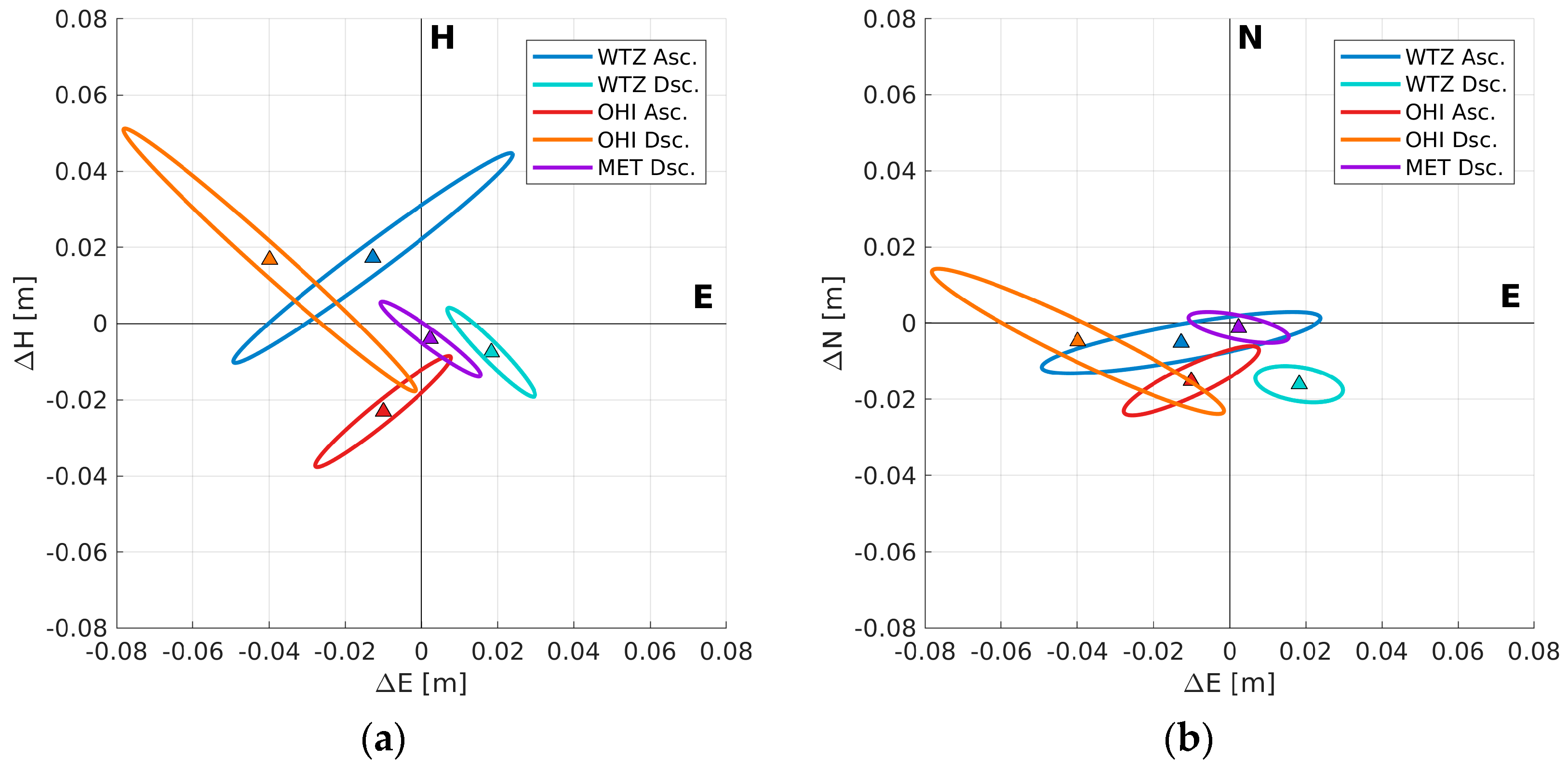
Another interesting aspect is the overall error distribution of the coordinate solution, namely the error ellipsoid, which is visualized in Figure 9. Because of the same scaling for a confidence level of 95%, the horizontal and vertical cross sections shown in the graphics directly correspond to the confidence values listed in Table 7. The $\sigma N$, $\sigma E$, $\sigma H$ are simply the bounding boxes of the ellipses, while the smallest errors are found to be in the range direction, see Figure 9a. All the ellipses are inclined to about 40 degrees, which is the average incidence angles of the passes for the individual CRs, see the angles listed in Table 5. As expected, the underlying intersection geometries are most sensitive in the SAR range direction, and least sensitive in the perpendicular cross-range direction. The horizontal view, see Figure 9b, has a similar behavior, but here it is the azimuth that dominates the orientation. The smaller axes coincide with the local sensor heading, which is nearly north-south due to the sun-synchronous orbit used by TerraSAR-X [29]. Only towards the polar regions, the tracks start to converge, leading to the slightly more tilted horizontal error ellipses of the CRs at GARS O’Higgins. Therefore, the azimuth is almost only sensitive for the north-south component. These error patterns also explain the different confidence levels derived for local north, east and height (Table 5), and they make it immediately clear, why the ideal setup for the application of SAR positioning is a reflector with a common phase center for ascending and descending passes. This concept was already studied with TerraSAR-X in a small experiment at Wettzell [30].

In summary, the 3-D localization experiments underline the very high absolute accuracy that can be achieved with absolute SAR positioning under ideal circumstances. Moreover, they confirm the performance of our positioning method, the high quality TerraSAR-X radar payloads, the fidelity of the SAR processing, as well as the accuracy of the annotated orbit product.

5. Discussion

In the previous section, we analyzed the geolocation performance of TerraSAR-X with respect to a multitude of contributing parameters: polarization, incidence angle, the pass direction (ascending, descending), the occurrence of long-term trends, and geographic target location. Due to the large amount of topics, the straightforward way of presentation was to discuss each of these aspects in the immediate context of the corresponding measurement results. In order to synthesize these discussions, two comprehensive aspects shall be addressed here. Firstly, we compare the determined a posteriori location error with the a priori error computed from the expected amount of the major error contributions. Secondly, we want to give an outlook on an upcoming further improvement in the attainable geolocation accuracy which is enabled by a new approach in precise orbit determination.

5.1. Analysis of Error Contributions

Table 8. Estimations for the major error contributions in the geolocation result.

Parameter	Azimuth Contribution [mm]	Range Contribution [mm]
Clutter	0.3‒12 1	0.7‒6 1
Tropospheric delay	‒	0.5‒1.3 2
Ionospheric delay	‒	1.5‒5.3 2
Timing and ADC sample rate	7	<3
(Science) Orbit	<50 3	<50 3

¹ Mainly depending on CR size (1.5 or 0.7 m) and imaging mode (ST300 or HS300). ² Depending on test site and incidence angle. ³ Conservative assumption.

shows a priori estimates for the major contributions to the location error. The estimate for the clutter contribution results from Equation (3), while the estimates for the measurement accuracy of tropospheric and ionospheric delay are taken from the respective data products. Considering the methods discussed in [27], the assumed uncertainty in the azimuth timing, taken from L1B annotation of operational TerraSAR-X products, amounts to about 1 microsecond, corresponding to about 7 mm azimuth error. The Analog to Digital Converter (ADC) sample rate of both TerraSAR-X sensors (about 330 MHz) is operationally monitored to ascertain that the difference between its actual and annotated value does not exceed a margin of 1 Hz. In this way, the residual uncertainty in the ADC sample rate contributes at most 3 mm to the overall ranging error. A conservative estimate for the actual orbit error of TerraSAR-X Science orbits is given in [31].

Comparing the error contributions listed in Table 8, the residual uncertainty in the knowledge of the precise orbit is the dominant contribution in our CRs measurement series (whereas for weaker targets the clutter contribution would be higher and might dominate there). However, as long as we only know an upper limit for the actual orbit error, there remains room for interpretation what could be its true contribution. Regarding the localization accuracies we obtained in our measurement series, we conclude that the actual orbit error must be significantly below the estimated upper limit of 5 cm and that it may amount to about 1 cm.

5.2. Geolocation Improvements from More Precise Orbit Determination

Beyond the currently used TerraSAR-X Science orbits, [28] discusses methods to further improve the accuracy of the orbit determination. Once operationally applied, the geolocation accuracy of SAR immediately should benefit from these improvements. We tested the new experimental orbit solutions by repeating our location accuracy measurements in a modified way where we computed the expected radar time coordinates on base of these orbits instead of using the operational TerraSAR-X Science orbit products.

Table 9. Comparison of the mean values and standard deviations in azimuth and range for operational Science orbits (as they are already shown in Table 6) and for the new experimental TerraSAR-X orbit solutions discussed in [28] (operationally not accessible as yet).

Measurement Series	Azimuth Offset [mm]		Range Offset [mm]
	Science Orbits	Experimental Orbits	Science Orbits	Experimental Orbits
Wettzell Asc.	‒3.2 ± 17.7	‒6.1 ± 13.4	‒25.7 ± 11.6	‒10.2 ± 7.6
Wettzell Desc.	+13.1 ± 24.3	+12.9 ± 22.7	‒13.0 ± 13.4	‒9.2 ± 9.8
GARS O’Higgins Asc.	‒5.4 ± 24.4	‒2.2 ± 28.5	+1.1 ± 17.6	+2.4 ± 14.5
GARS O’Higgins Desc.	+21.8 ± 22.1	+18.5 ± 17.6	+3.2 ± 14.5	+1.4 ± 14.0
Metsähovi Desc.	+0.2 ± 17.5	‒0.4 ± 15.0	‒1.9 ± 12.0	0.0 ± 9.1

and Figure 10 show the detailed CR-wise mean values and standard deviations (1σ) of the obtained measurement results and oppose them to the results previously obtained with the operational Science orbits. As a finding of this experiment, we observed that for the 1.5 m CRs the usage of the new orbit solutions TerraSAR-X significantly lowers the standard deviations. They amount to about 1.5 cm in azimuth while in range sub-centimeter level is reached. This represents an accuracy gain of 15% in azimuth and 28% in range compared to the usage of the operational Science orbits. In case of the 0.7 m CRs, where also the clutter significantly contributes to the total location error, the accuracy gain from the improved orbit quality is naturally less distinct (1.5% in azimuth and 10% in range).

Consequently, also the stereo SAR solutions for the CR coordinates profit from the increased orbit quality.

Table 10. Differences of the TerraSAR-X coordinates using the updated orbits and the reference coordinates in the global ITRF2014 expressed in local north, east and height. The variances of the TerraSAR-X solution mark the 95% confidence interval of the estimated coordinates.

Measurement Series	ΔN [mm]	ΔE [mm]	ΔH [mm]	σN [mm]	σE [mm]	σH [mm]
Wettzell Ascending	‒9.0	‒18.8	+0.1	+6.0	+23.5	+17.9
Wettzell Descending	‒14.3	+11.9	‒1.1	+4.2	+9.1	+9.2
GARS O’Higgins Ascending	‒6.3	‒4.6	‒14.1	+9.0	+17.3	+14.1
GARS O’Higgins Descending	‒8.4	‒24.4	+10.9	+17.0	+34.4	+30.9
Metsähovi Descending 1	+1.8	‒7.8	+5.6	+3.5	+11.4	+8.5

¹ The reason, why the differences are almost zero, is that we used the Metsähovi CR as calibration reference for all of our test sites, see Section 4.2.

shows the differences of the SAR measured 3-D coordinates using the new orbits and the GNSS reference coordinates. Figure 11 visualizes a comparison between the results obtained with operational science orbits (which were shown in Table 7) and the results for the new orbits. A closer look on the diagram reveals that the new orbits lead to improvements in almost all the estimated accuracies and the coordinate differences become smaller, in particular the height is now more accurately determined; only at Wettzell there remain significant millimeter level differences for the horizontal positions.

6. Conclusions

With the setup of three CR test sites as far apart from each other as Germany, Finland and the Antarctic Peninsula, we established a far-distributed test network to verify the absolute localization accuracy of space borne SAR sensors and the worldwide reproducibility of the obtained results. The vicinity of all of our test sites to local IGS reference stations allows very precise determination of the CRs’ reference coordinates relative to the respective station ties by terrestrial survey. These precise reference coordinates render a new class of SAR calibration and validation accuracy possible.

Based on our test network, absolute geolocation accuracy at better than centimeter level is proven for both TerraSAR-X sensors (TSX-1 and TDX-1). Prerequisite for such high localization accuracy is meticulous care in processing and calibration of the SAR data and the thorough correction of location measurements from a SAR image for wave propagation effects and for Earth dynamics, consistent with the methods applied in geodesy. In contrast to the “out of the box” usage of TerraSAR-X data, additional external data sources, which are well established in the area of GNSS, have to be accessed in order to obtain precise correction values for atmospheric signal propagation delays. In the process, the geometric instrument calibration constants had to be adapted to the altered measurement approach.

Handling SAR as a geodetic measurement instrument opens completely new application areas for SAR. First examples were already discussed in the literature, e.g., the efficient survey of landmarks along road networks [32] or the stereo measurement of building heights [33]. The synergetic usage of geodetic SAR and SAR tomography is discussed in [34].

References

- Schubert, A.; Jehle, M.; Small, D.; Meier, E. Mitigation of Atmosphere Perturbations and Solid Earth Movements in a TerraSAR-X Time Series. J. Geod. 2011, 86, 257–270. [Google Scholar] [CrossRef]
- Balss, U.; Cong, X.Y.; Brcic, R.; Rexer, M.; Minet, C.; Breit, H.; Eineder, M.; Fritz, T. High Precision Measurement on the Absolute Localization Accuracy of TerraSAR-X. In Proceedings of the 2012 IEEE International Geoscience & Remote Sensing Symposium (IGARSS), Munich, Germany, 22–27 July 2012; pp. 1625–1628. [Google Scholar]
- Balss, U.; Gisinger, C.; Cong, X.Y.; Brcic, R.; Hackel, S.; Eineder, M. Precise Measurements on the Absolute Localization Accuracy of TerraSAR-X on the Base of Far-Distributed Test Sites. In Proceedings of the 10th European Conference on Synthetic Aperture Radar (EUSAR), Berlin, Germany, 3–5 June 2014; pp. 993–996. [Google Scholar]
- Capaldo, P.; Fratarcangeli, F.; Nascetti, A.; Mazzoni, A.; Porfiri, M.; Crespi, M. Centimeter Range Measurement Using Amplitude Data of TerraSAR-X Imagery. In Proceedings of the ISPRS Technical Commission VII Symposium, Istanbul, Turkey, 29 September–2 October 2014; pp. 55–61. [Google Scholar]
- Altamimi, Z.; Rebischung, P.; Métivier, L.; Collilieux, X. ITRF2014: A New Release of the International Terrestrial Reference Frame Modeling Nonlinear Station Motions. J. Geophys. Res. Solid Earth 2016, 121, 6109–6131. [Google Scholar] [CrossRef]
- Schubert, A.; Small, D.; Jehle, M.; Meier, E. COSMO-SkyMed, TerraSAR-X, and RADARSAT-2 Geolocation Accuracy after Compensation for Earth-System Effects. In Proceedings of the 2012 IEEE International Geoscience & Remote Sensing Symposium (IGARSS), Munich, Germany, 22–27 July 2012; pp. 3301–3304. [Google Scholar]
- Petit, G.; Luzum, B. IERS Conventions (2010); IERS Technical Note 36; Verlag des Bundesamtes für Kartographie und Geodäsie: Frankfurt, Germany, 2010. [Google Scholar]
- Hofmann-Wellenhof, B.; Lichtenegger, H.; Wasle, E. GNSS Global Navigation Satellite Systems; Springer: Vienna, Austria, 2008; ISBN 978-3-211-73012-6. [Google Scholar]
- Meindl, M.; Dach, R.; Jean, Y. International GNSS Service Technical Report 2011; Astronomical Institute University of Bern: Bern, Switzerland, 2012. [Google Scholar]
- Balss, U.; Gisinger, C.; Cong, X.Y.; Brcic, R.; Steigenberger, P.; Eineder, M.; Pail, R.; Hugentobler, U. High Resolution Geodetic Earth Observation with TerraSAR-X: Correction Schemes and Validation. In Proceedings of the 2013 IEEE International Geoscience & Remote Sensing Symposium (IGARSS), Melbourne, Australia, 21–26 July 2013; pp. 4499–4502. [Google Scholar]
- Cumming, I.G.; Wong, F.H. Digital Processing of Synthetic Aperture Radar: Algorithms and Implementations; Artech House: Boston, MA, USA, 2005; ISBN 978-1-580-53058-3. [Google Scholar]
- Gisinger, C.; Balss, U.; Pail, R.; Zhu, X.X.; Montazeri, S.; Gernhardt, S.; Eineder, M. Precise Three-Dimensional Stereo Localization of Corner Reflectors and Persistent Scatterers With TerraSAR-X. IEEE Trans. Geosci. Remote Sens. 2015, 53, 1782–1802. [Google Scholar] [CrossRef]
- Mikhail, E.M.; Ackermann, F. Observations and Least Squares; IEP-Dun-Donnelly, Harper and Row: New York, NY, USA, 1976. [Google Scholar]
- Koch, K.R.; Kusche, J. Regularization of geopotential determination from satellite data by variance components. J. Geod. 2012, 76, 259–268. [Google Scholar] [CrossRef]
- Koch, K.R. Parameter Estimation and Hypotheses Testing in Linear Models; Springer: Berlin/Heidelberg, Germany, 1999; ISBN 978-3-642-08461-4. [Google Scholar]
- Gray, A.L.; Vachon, P.W.; Livingstone, C.E.; Lukowski, T.I. Synthetic Aperture Radar Calibration Using Reference Reflectors. IEEE Trans. Geosci. Remote Sens. 1990, 28, 374383. [Google Scholar] [CrossRef]
- Bamler, R.; Eineder, M. Accuracy of Differential Shift Estimation by Correlation and Split-Bandwidth Interferometry for Wideband and Delta-k SAR Systems. Geosci. Remote Sens. Lett. 2005, 2, 151–155. [Google Scholar] [CrossRef]
- Stein, S. Algorithms for Ambiguity Function Processing. IEEE Trans. Acoust. Speech Signal Process. 1981, ASSP-29, 588–599. [Google Scholar] [CrossRef]
- Swerling, P. Radar Measurement Accuracy. In Radar Handbook; Skolnik, M., Ed.; McGraw-Hill: New York, NY, USA, 1970; pp. 4:1–4:14. [Google Scholar]
- Schubert, A.; Small, D.; Gisinger, C.; Balss, U.; Eineder, M. Corner Reflector Deployment for SAR Geometric Calibration and Performance Assessment; ESRIN: Frascati, Italy, 2018; in press. [Google Scholar]
- Balss, U.; Gisinger, C.; Eineder, M.; Breit, H.; Schubert, A.; Small, D. Survey Protocol for Geodetic SAR Sensor Analysis; ESRIN: Frascati, Italy, 2018; in press. [Google Scholar]
- Schwerdt, M.; Bräutigam, B.; Bachmann, M.; Döring, B.; Schrank, D.; Gonzalez, J.H. Final TerraSAR-X Calibration Results Based on Novel Efficient Methods. IEEE Trans. Geosci. Remote Sens. 2010, 48, 677–689. [Google Scholar] [CrossRef]
- Breit, H.; Fritz, T.; Balss, U.; Lachaise, M.; Niedermeier, A.; Vonavka, M. TerraSAR-X Processing and Products. IEEE Trans. Geosci. Remote Sens. 2010, 48, 727–739. [Google Scholar] [CrossRef]
- Fritz, T.; Eineder, M. TerraSAR-X Ground Segment Basic Product Specification Document. Available online: http://sss.terrasar-x.dlr.de/docs/TX-GS-DD-3302.pdf (accessed on 15 February 2018).
- EOWEB Earth Observation on the WEB. Available online: https://centaurus.caf.dlr.de:8443 (accessed on 16 February 2018).
- TerraSAR-X Science Service System. Available online: http://sss.terrasar-x.dlr.de (accessed on 26 February 2018).
- Balss, U.; Breit, H.; Fritz, T.; Steinbrecher, U.; Gisinger, C.; Eineder, M. Analysis of Internal Timings and Clock Rates of TerraSAR-X. In Proceedings of the 2014 IEEE International Geoscience & Remote Sensing Symposium (IGARSS), Quebec, QC, Canada, 13–18 July 2014; pp. 2671–2674. [Google Scholar]
- Hackel, S.; Gisinger, C.; Balss, U.; Wermuth, M.; Montenbruck, O. Long-Term Validation of TerraSAR-X Orbit Solutions with Laser and Radar Measurements. Remote Sens. Spec. 2018, in press. [Google Scholar]
- Werninghaus, R.; Buckreuss, S. The TerraSAR-X Mission and System Design. IEEE Trans. Geosci. Remote Sens. 2010, 48, 606–614. [Google Scholar] [CrossRef] [Green Version]
- Gisinger, C.; Willberg, M.; Balss, U.; Klügel, T.; Mähler, S.; Pail, R.; Eineder, M. Differential geodetic stereo SAR with TerraSAR-X by exploiting small multi-directional radar reflectors. J. Geod. 2017, 91, 53–67. [Google Scholar] [CrossRef]
- Yoon, Y.; Eineder, M.; Yague-Martinez, N.; Montenbruck, O. TerraSAR-X Precise Trajectory Estimation and Quality Assessment. IEEE Trans. Geosci. Remote Sens. 2009, 47, 1859–1868. [Google Scholar] [CrossRef]
- Runge, H.; Balss, U.; Suchandt, S.; Klarner, R.; Cong, X.Y. DriveMark—Generation of High Resolution Road Maps with Radar Satellites. In Proceedings of the 11th ITS European Congress, Glasgow, UK, 6–9 June 2016; pp. 1–6. [Google Scholar]
- Eldhuset, K.; Weydahl, D.J. Geolocation and Stereo Height Estimation Using TerraSAR-X Spotlight Image Data. IEEE Trans. Geosci. Remote Sens. 2011, 49, 3574–3581. [Google Scholar] [CrossRef]
- Zhu, X.X.; Montazeri, S.; Gisinger, C.; Hanssen, R.F.; Bamler, R. Geodetic SAR Tomography. IEEE Trans. Geosci. Remote Sens. 2016, 54, 18–35. [Google Scholar] [CrossRef]
Figure 1.
Schematic view of measurement arrangement and procedures.
Figure 2.
Corner reflectors at our test sites: (a) Wettzell, Germany; (b) GARS O’Higgins, Antarctic Peninsula; (c) Metsähovi, Finland.
Figure 3.
Temporal progression of the azimuth (blue) and range (red) offset obtained at the Metsähovi test site.
Figure 4.
Temporal progression of the azimuth (blue) and range (red) offset obtained at the Wettzell test site: (a) Wettzell Ascending measurement series; (b) Wettzell Descending.
Figure 5.
Temporal progression of the azimuth (blue) and range (red) offset obtained at the GARS O’Higgins test site: (a) GARS O’Higgins Ascending measurement series; (b) GARS O’Higgins Descending.
Figure 6.
Gradients of the interpolated linear trends at the different test sites: (a) range; (b) azimuth. The plotted error bars represent a 95% confidence interval (2σ).
Figure 7.
Scatter plots of the obtained azimuth and range offsets: (a) Wettzell Ascending; (b) Wettzell Descending; (c) GARS O’Higgins Ascending; (d) GARS O’Higgins Descending; (e) Metsähovi Descending.
Figure 8.
Close-up of the temporal progression of the obtained azimuth (a) and range (b) offset at the Wettzell test site during the ST300 campaign (yellow) interleaving regular HS300 acquisitions (green).
Figure 9.
Differences of the TerraSAR-X stereo coordinates to the reference coordinates, and the error ellipsoid of the SAR solution scaled to 95% confidence level: Horizontal cross section in local east/height (a); vertical cross section in local north/east (b). WTZ = Wettzell, OHI = GARS O’Higgins and MET = Metsähovi.
Figure 10.
Comparison of the mean values (a) and standard deviations (b) in azimuth and range for operational Science orbits (values of Table 6) and new experimental orbits (values of Table 9). The different colors represent the different measurement series.
Figure 11.
Comparison of the biases (a) and 95% confidence intervals (b) in north, east and height for operational Science orbits (values of Table 7) and new experimental orbits (values of Table 10). The different colors represent the different measurement series.