Discrimination of Algal-Bloom Using Spaceborne SAR Observations of Great Lakes in China
by
 ,
,
Lin Wu
1,2 ,
,
Le Wang
1,
Lin Min
3,
Wei Hou
1,
Zhengwei Guo
1,4,*,
Jianhui Zhao
1,4,* and
Ning Li
1,4 1
College of Computer and Information Engineering, Henan University, Kaifeng 475004, China
2
College of Environment and Planning, Henan University, Kaifeng 475004, China
3
Network Information Center Office, Henan University, Kaifeng 475004, China
4
Laboratory of Spatial Information Processing, Henan University, Kaifeng 475004, China
*
Authors to whom correspondence should be addressed.
Remote Sens. 2018, 10(5), 767; https://doi.org/10.3390/rs10050767
Submission received: 4 April 2018
/
Revised: 5 May 2018
/
Accepted: 13 May 2018
/
Published: 16 May 2018
(This article belongs to the Special Issue Satellite Remote Sensing for Water Resources in a Changing Climate)
Abstract
:Although optical remote sensing can intuitively detect algal bloom, it is limited by the weather conditions. Synthetic aperture radar (SAR) is not affected by inadequate weather conditions. According to visual interpretation of SAR images and comparisons of quasi-synchronized optical images, the gathering areas of algal bloom present as “dark regions” on SAR images. It is shown that using SAR to monitor the water surface is workable. However, dark regions may also be caused by other factors, such as low wind speeds. This challenges with SAR monitoring of algal bloom on the water surface. In this study, an improved K-means algorithm, combined with multi-Otsu thresholding algorithm, was proposed to segment the dark regions. After feature analysis and extraction of Sentinel-1A images, an algal bloom recognition model with a support vector machine (SVM) was applied to discriminate the algal bloom dark regions from the low wind dark regions. According the experimental results, the overall accuracy achieved 74.00% in Taihu Lake. Additionally, this method was also validated in Chaohu Lake and Danjiangkou Reservoir. Therefore, it can be concluded that SAR can provide a new technical means for monitoring algal bloom of inland lakes, particularly when it is cloudy and unsuitable for optical remote sensing. To obtain more information about algal bloom, multi-band and multi-polarization SAR images can be considered for future.
1. Introduction
In recent decades, the intensification of human activities in lake basins and surrounding areas has caused large amounts of nutrients flowing into the lake through various channels, which results in surges of eutrophication levels and frequent algal bloom. The demise and decomposition of algal bloom consume a large amount of dissolved oxygen in the water, and seriously damage the ecological balance of the water body, which has a very detrimental impact on aquaculture [1] and daily activities [2]. In recent years, large-scale algal bloom frequently outbreak in freshwater lakes in China, such as Taihu Lake and Chaohu Lake. Thus, remote sensing monitoring of algal bloom has become an important issue in many fields of science, such as water environment and ecology [3,4].
Due to the sensitivity of spectral features and the maturity of remote sensing image processing technologies, optical images can directly show information about algal blooms, such as the areas, positions, and dynamic changes. However, optical images are greatly affected by the meteorological conditions, such as clouds, rain, and fog. Furthermore, it is impossible to image at night or provide all-day data, which seriously affect the practicability of scientific research. For example, on 29 May 2007, a large-scale outbreak of cyanobacterial blooms in Taihu Lake caused the deterioration of the water, and threatened the domestic water supply of Wuxi [5]. Within the week of the bloom, Taihu Lake was completely covered by clouds for three days, and partially covered for four days. At that time, the MODerate-resolution Imaging Spectroradiometer (MODIS) could not provide any information about algal bloom.
Until now, most studies on the monitoring and recognition of algal bloom focus on the processing of optical images, and are mainly based on two methods, which are band fusion and thresholding [6,7,8,9,10,11]. Hu et al. [12] successfully extracted cyanobacteria bloom areas in Taihu Lake using the floating algae index (FAI) based on three MODIS bands. Based on FAI, researchers improved the traditional methods and models, and gave the optimal combination of optical bands for monitoring Taihu Lake, Donting Lake, Poyang Lake, Erhai Lake, and other inland lakes in China. In addition, they obtained the spatial and temporal distributions of algal bloom in those lakes [13,14,15,16,17]. However, the researches based on SAR image are still in the initial stages. Wang Ganlin et al. [18] used multi-temporal SAR images to monitor algal bloom. By a simultaneous field survey, they confirmed that the gathering of algae and viscous secretions, during the outbreak of cyanobacterial blooms in Taihu Lake, resulted in a reduction of the radar backscattering coefficient, generating a large number of dark regions on SAR images. Sieburth et al. [19] found that a layer of an oil-like substance formed on the water surface during the outbreak of algal bloom. These oil films have a large damping effect on capillary waves, thus presenting as significant dark regions on SAR images. Using SAR images, Alpers et al. [20] studied the oil films of the water surface, and found that the oil film can reduce the radar backscattering coefficient by 6–17 dB. Gade et al. [21] analyzed different types of films on the water surface with low wind speed (), and distinguished them using multi-band and multi-polarization SIR-C/X SAR images. By using ASAR and MODIS images, Wang Ji et al. [22] found that dark regions on SAR images were highly consistent with algal bloom areas on MODIS images. However, they did not explain the causes of other similar non-bloom dark regions on SAR image. Wang et al. [23] used optical images, including MODIS and HJ-CCD, and SAR images, including ERS-2 and ENVISAT ASAR, to monitor cyanobacterial blooms in inland lakes based on the maximum gradient complexity method. However, they did not solve the problem of automated processing of SAR images. By using MERIS and ASAR images, Bresciani et al. [24] firstly gave the relationship between the chlorophyll concentration and the backscattering coefficient during the cyanobacterial blooms in the Curonian Lagoon in Europe, but the correlation was too weak to be accurate.
In this paper, a method for algal bloom recognition based on SAR images is presented. By exploiting different image features, including gray levels, geometry, and texture, a supervised learning classification mechanism is built to recognize algal bloom. The experimental results show that the proposed method has a high recognition accuracy and practical meaning for SAR monitoring of algal bloom.
2. Case Study
2.1. Study Areas and Images
The second national survey of lakes in China showed that 85.40% of the 138 lakes exceeded the eutrophication standard. In addition, 40.10% of the lakes reached to severe eutrophication standard [25].
As shown in Figure 1, Taihu Lake (30°56′N–31°33′N, 119°52′E–120°37′E) has a water surface area of 2338 km2 and an average depth of 1.9 m. Its water quality is closely related to the agricultural irrigation and aquaculture activities in surrounding cities, such as Suzhou, Huzhou, Wuxi, and Yixing [26,27]. Chaohu Lake (31°25’N–31°43’N, 117°16’E–117°51’E) is located in the central part of Anhui Province, and has a water surface area of approximately 760 km2 and a maximum water depth of 7.98 m. Danjiangkou Reservoir (32°36’N–31°33’N, 110°59’E–111°49’E) crosses Henan and Hubei provinces, and consists of Hanjiang Reservoir and Danjiang Reservoir. It has a water surface area of approximately 600 km2 and a storage capacity of approximately 29.05 billion cubic meters. This reservoir is the water source for the middle route of the South-to-North Water Diversion Project [28,29,30,31,32], which is the largest water resources distribution project of China. The project benefits more than 200 million people in 14 cities of four provinces.
In recent years, algal bloom has occurred frequently in Taihu Lake and Chaohu Lake, and seriously affected the quality of the water consumed by the surrounding residents. Rapid and effective remote sensing monitoring of the water environment of these two lakes are urgently required. Although algal bloom has not emerged in Danjiangkou Reservoir, slight eutrophication has occurred in some tributaries. Monitoring the water quality via remote sensing and preventing pollution are the tasks that cannot be ignored. Therefore, this reservoir is also as one of our study areas.
The Sentinel-1A satellite, the Earth observation satellite of the European Space Agency’s Copernicus Initiative, launched on 3 April 2014, and became officially operational in May 2015. The radar sensor works at the C-band. VV polarization and Interferometric Wide-swath mode are chosen in this study. The swath width is 250 km, and the resolution is 5 m × 20 m.
Under the same conditions, there is a great difference in the radar reflected waves of the same ground object from different polarization modes. On a basis of literatures investigating, it can be known that VV polarization is better than that of HH polarization [33], aimed at the monitoring of water surface. That is the reason why we selected VV polarization for algal bloom monitoring.
The MODIS sensor has been widely used in global environmental monitoring. It consists of 36 spectral bands, and has resolutions of 250 m, 500 m, and 1000 m. The Landsat-8 satellite was launched by NASA in February 2013, and the Operational Land Imager (OLI) includes nine bands with 30 m resolution. In this study, Landsat-8 and MODIS optical images were quasi-synchronized with SAR images, and used to assist the interpretation of SAR images.
2.2. Image Preprocessing
In this study, ENVI 5.3 (Exelis Visual Information Solutions Company: Boulder, CO, USA) was used to preprocess the optical images. And SAR images were preprocessed with SNAP, a free software, provided by the European Space Agency (Paris, France).
2.2.1. Preprocessing of Sentinel-1A Images
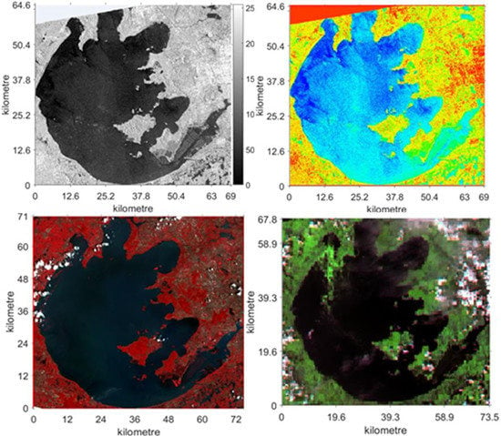
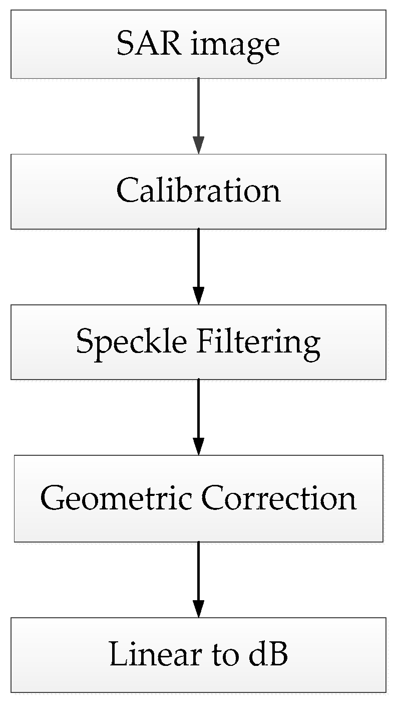
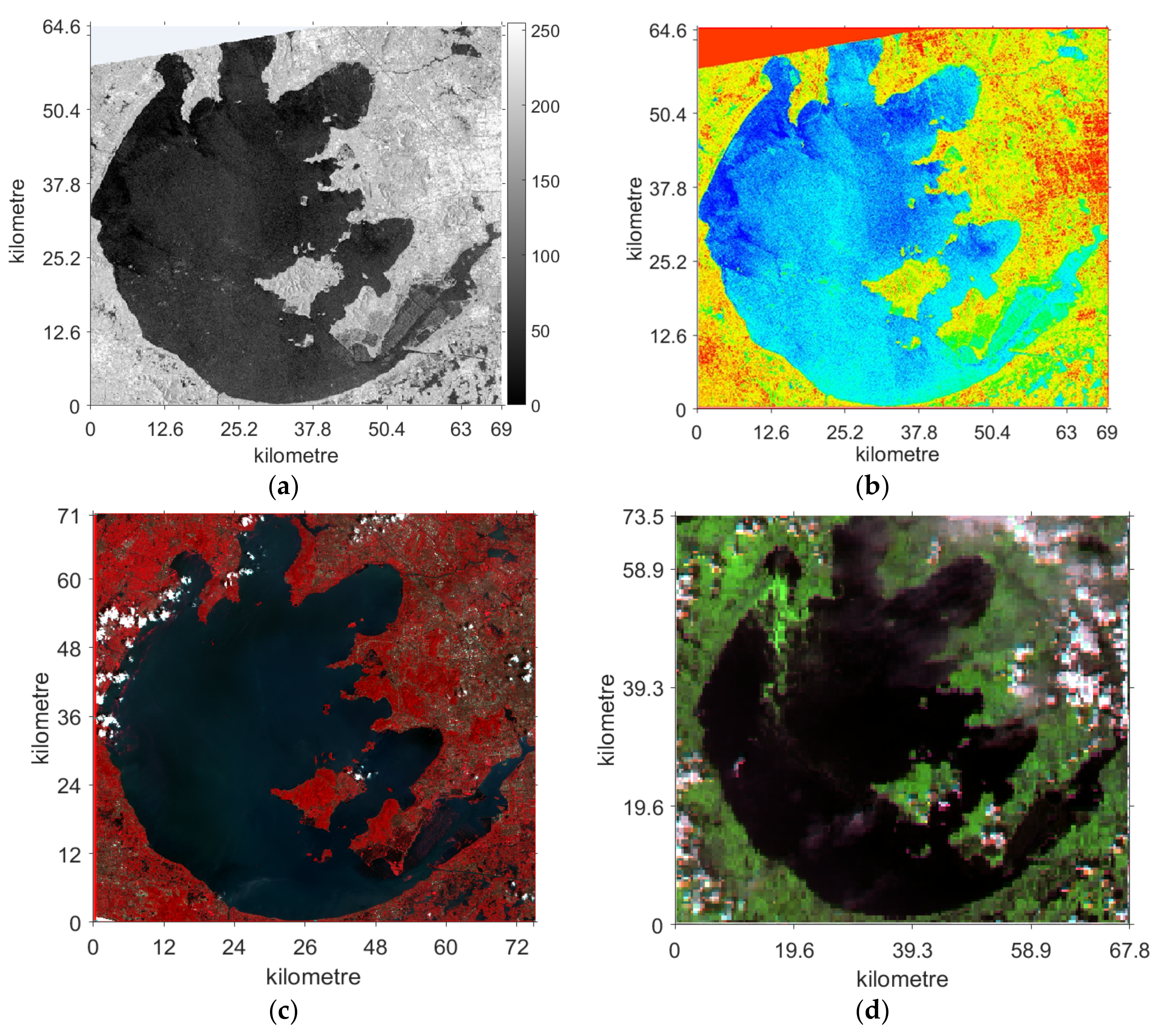
The preprocessing procedures are shown in Figure 3, including calibration, speckle filtering, geometric correction, and linear to dB. The calibration process involved radiometric correction to reduce the radiation deviation. A refined Lee filter with a window size 7 × 7 was used for despeckling. A range Doppler terrain correction operator was used to reduce the deviation caused by geometric distortion. The type of digital elevation model used is SRTM 3Sec. The process of linear-to-dB enhances the image contrast to simplify the identification of the dark regions. Figure 4a is an example of preprocessed SAR images. In order to better display the algal bloom in Figure 4a, the gray-color transform [34] was used to obtain the false color image, as shown in Figure 4b.
2.2.2. Preprocessing of Landsat-8 Images
The universal radiometric calibration tool (radiometric calibration) was applied to calibrate the output radiance for Landsat-8 images. Then, the Fast Line-of-sight Atmospheric Analysis of Spectral Hypercubes (FLAASH) model was used for atmospheric correction. No geometric correction was necessary because the Level 1 GeoTIFF Data Product is terrain-corrected with DEM. Thus, the coordinate accuracy met the small-scale requirements.
After preprocessing, the image contained 7 bands. Band 5, Band 4, and Band 3 were combined to form a false color RGB image, which presented as Figure 4c. It can be seen that the water is dark blue, and the color of vegetation is bright red.
2.2.3. Preprocessing of MODIS Images
The MODIS Level-1B (L1B) images were calibrated and atmospherically corrected using the MODIS Conversion Toolkit (MCTK). The radiometric calibration used the offsets and scales parameters of the HDF dataset. The pixel reflectivity can be calculated as:
where is the reflectivity scaling factor, is the digital number, and is the reflectivity scaling intercept.
The position information of the image was used for geometric correction. The projection used the Geographic Lat/Lon projection. After preprocessing, a false color RGB image was obtained by using Band 6, Band 2, and Band 1. Band 6 has 500 m resolution. Band 2 and Band 1 have 250 m resolution, resampled to 500 m resolution. Figure 4d is the output image after the false color synthesis, in which the green color represents the bloom floating on the water surface. In addition, other information, such as the position and area of algal bloom, can be obtained visually from the image.
2.3. Prior Information of the Dark Region in SAR Image
In order to verify the effectiveness of the proposed method, the prior information of the dark region on SAR image was used to determine the type of dark region.
It is known that the formation of algal bloom is relevant to the position, wind speed, and surroundings conditions. Li et al. [35] used the long time series MODIS images to monitor algal bloom of Taihu Lake, and found that the northern region is the hardest hit area of algal bloom, and the southern region and center of lake are moderate algal bloom around 2005. The above results are highly consistent with the conclusions of scholars such as Kong et al. [36,37]. The study of Yang [38] showed that algal bloom can drift with the wind. By the flume experiment, Bai et al. [39] proposed the conception of critical wind speed, which is 3.2 m/s. When the wind is below the critical speed, the algae drifts smoothly on water surface, and when the wind speed is faster than the critical wind speed, algae are mixed in water with the fluctuation of waves. The same conclusion was reached by Kong et al. [37]. They found that when the wind speed exceeds a certain range (3.1–3.2 m/s), the water surface is free of algal bloom, and the water surface appears with high gray levels on SAR images.
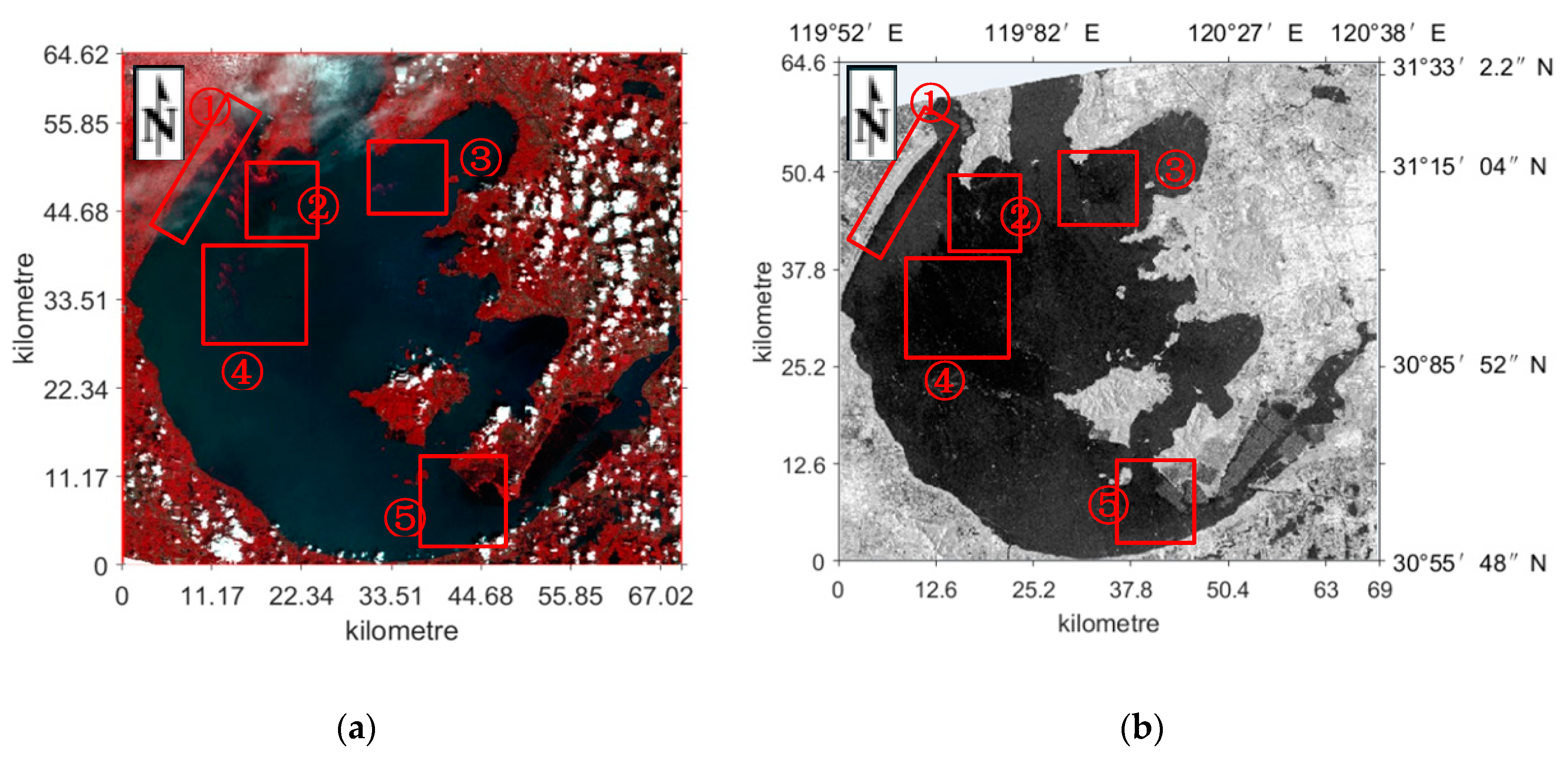
Based on the above conclusions, the field investigations were carried out in 2016 and 2017. The local environmental protection department in Wuxi provided the records of algal bloom in Taihu Lake, which confirmed the results of the literatures. Therefore, the study area of Taihu Lake was considered from four different types of areas, classified by the coverage of algal bloom. Figure 5 shows four types of areas by different colors.
Severe eutrophication areas: Meiliang Bay is close to the Wuxi city, and there are many tributaries in Zhushan Lake and Western coast. The nutrient-rich agricultural run-off and sewage contribute the aggregation of algal bloom. When the weather condition is suitable, these areas will be the harder-hit areas for the outbreak of algal bloom.
Moderate eutrophication areas: The areas include two regions. The one is the Southern Coast, which is close to the outlet of Taihu Lake. Due to the good fluidity of water, it is the moderate algal bloom area. Additionally, the other one is the center of Taihu Lake, whose terrain benefits the drift and diffusion of water bloom.
Light eutrophication areas: The region is in Gong Lake, located in the northeast of Taihu Lake. Gong Lake is the main water source of Suzhou and Wuxi. Additionally, there are no inflow rivers. Therefore, the water pollution here is relatively light.
Non-algal bloom areas: the regions are in Xu Lake, Donlim Tsui, and East Taihu Lake, located in the east of Taihu Lake. Due to an amount of water plants, water purification capacity is very high in these areas. In addition, the Center of Lake is also the non-algal bloom area, largely due to its position, which is a benefit to the drift and diffusion of algal blooms.
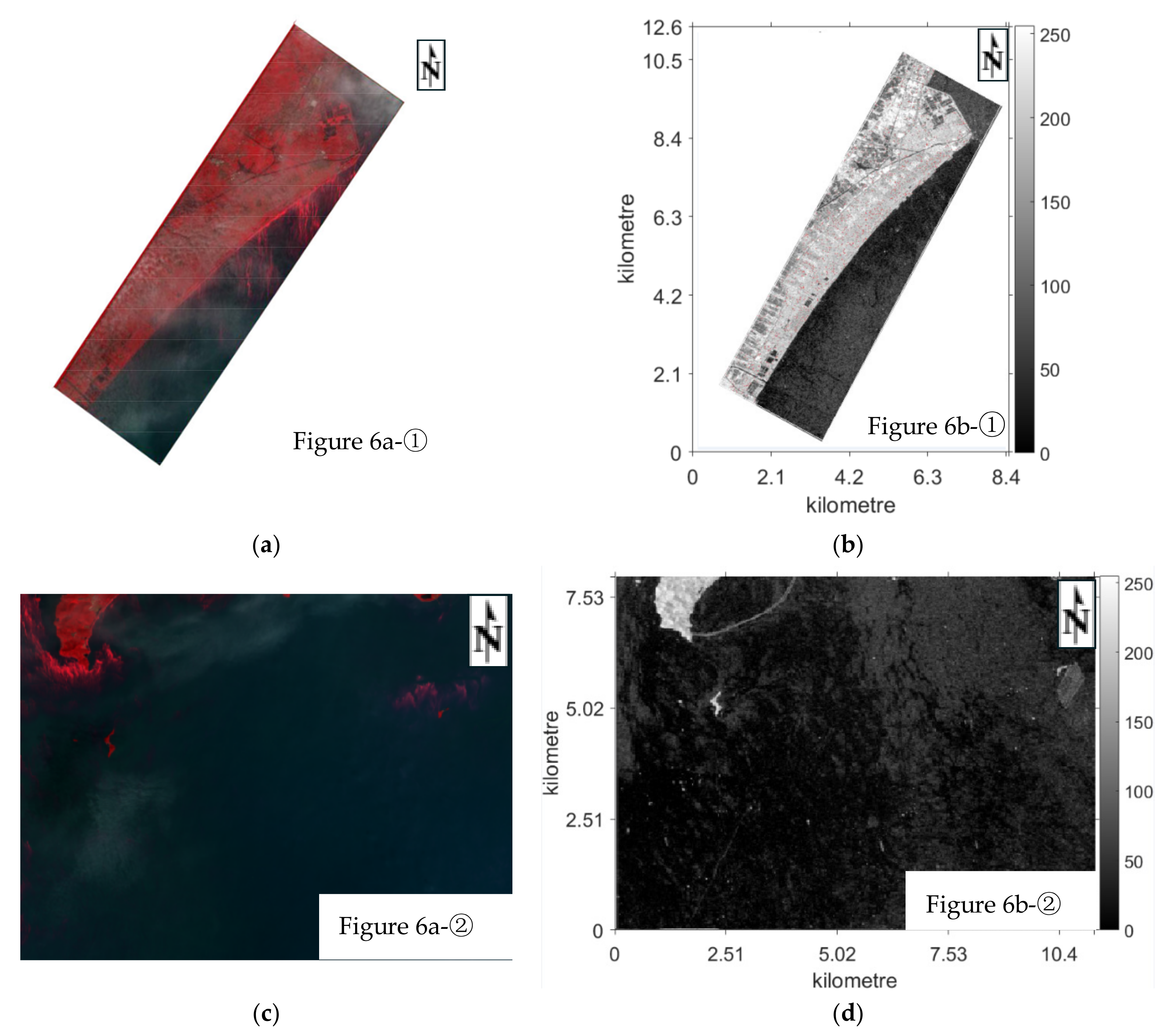
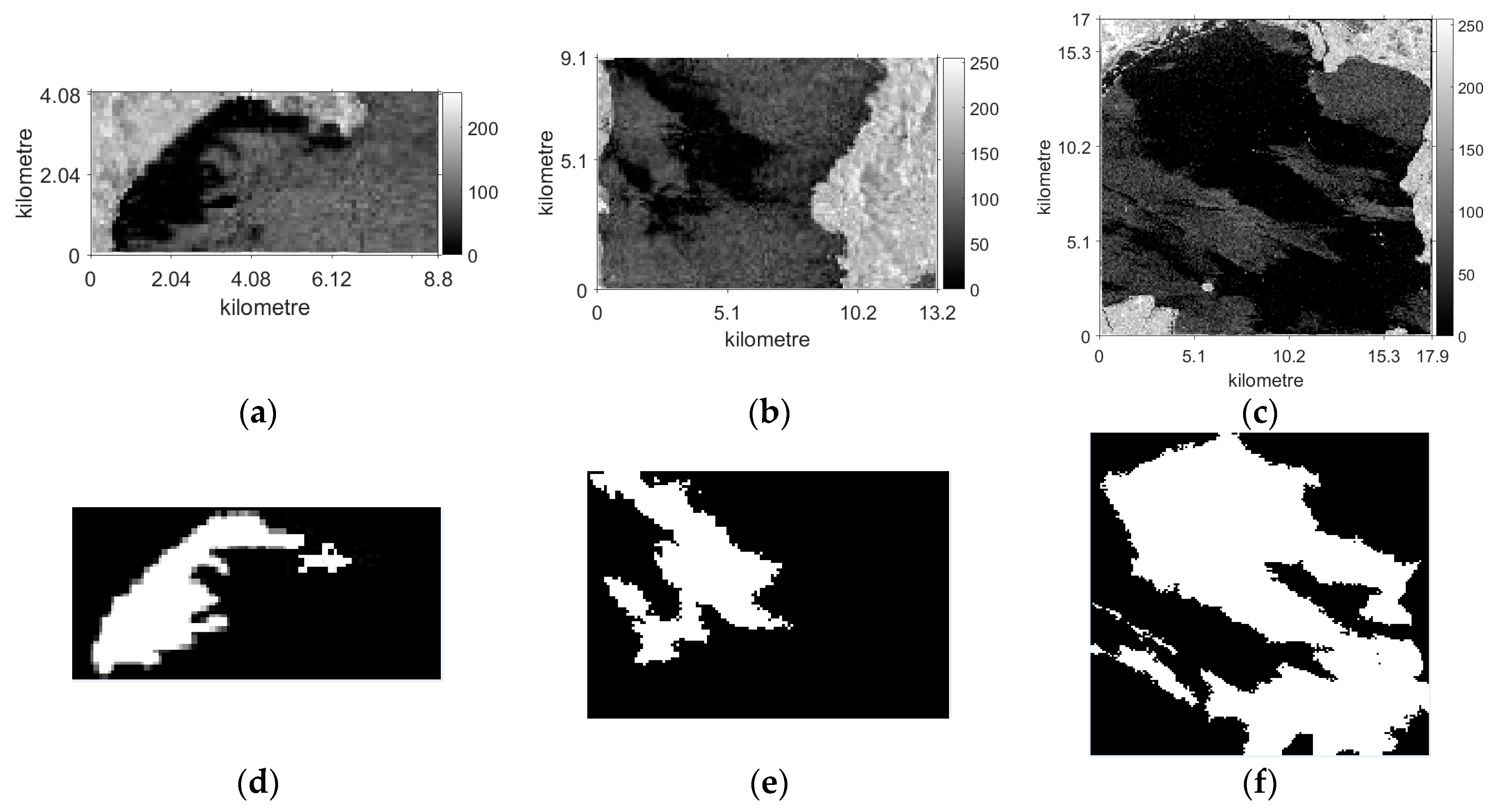
An example is given to illustrate the discrimination process of dark region using the above prior information. Figure 6 is a pair of optical and SAR image of Taihu Lake (30.55’48’’N–31.33’2.27’’N, 119.52’48’’E–120.38’24’’E). These two images, acquired in 11 September 2015, have a time interval of approximately 7 h. In Figure 6, five typical regions are marked with rectangles. The zoomed images of each region are shown in Figure 7.
In Figure 7a, it is easy to find the aggregation of algal bloom, although influenced by a few clouds. Considering that this region is in the severe eutrophication areas, the long dark region in Figure 7b is considered as the algal bloom regions.
Comparing Figure 7d with Figure 7c, the dark regions are a little closer to the north than the algal bloom regions. According to the meteorological information on 11 September 2015, there is a southeasterly wind at approximately 10:00 a.m. and the real-time wind speed is less than 2 m/s. Additionally, the shape of region ②, a nearly semicircular shore, contributes to the aggregation of algal blooms to some extent. Therefore, the dark regions in Figure 7d are considered as the algal bloom regions.
Large dark regions are visible in Figure 7h, compared with the same area in Figure 7g, which covers only a few dark regions in the west. According to the southwesterly wind with a speed of 2 m/s in the center of the lake, it can be concluded that part of the dark regions in Figure 7h are covered by algal blooms, which flow with the wind to the harbor, and most of the dark regions in Figure 7h are caused by low winds.
The location of region ⑤ is in the none-algal bloom areas, which is consistent with the status shown in Figure 7i. Although there are sparse dark regions in Figure 7j, it can be confirmed that it is not due to algal bloom.
To obtain the prior information of dark regions, several factors including location, meteorology, and optical images, are considered in the study. The prior information provides the basis for manual recognition of algal bloom dark region. The recognition accuracy of the proposed method is assessed by comparing with the results of manual recognition.
3. Materials and Methods
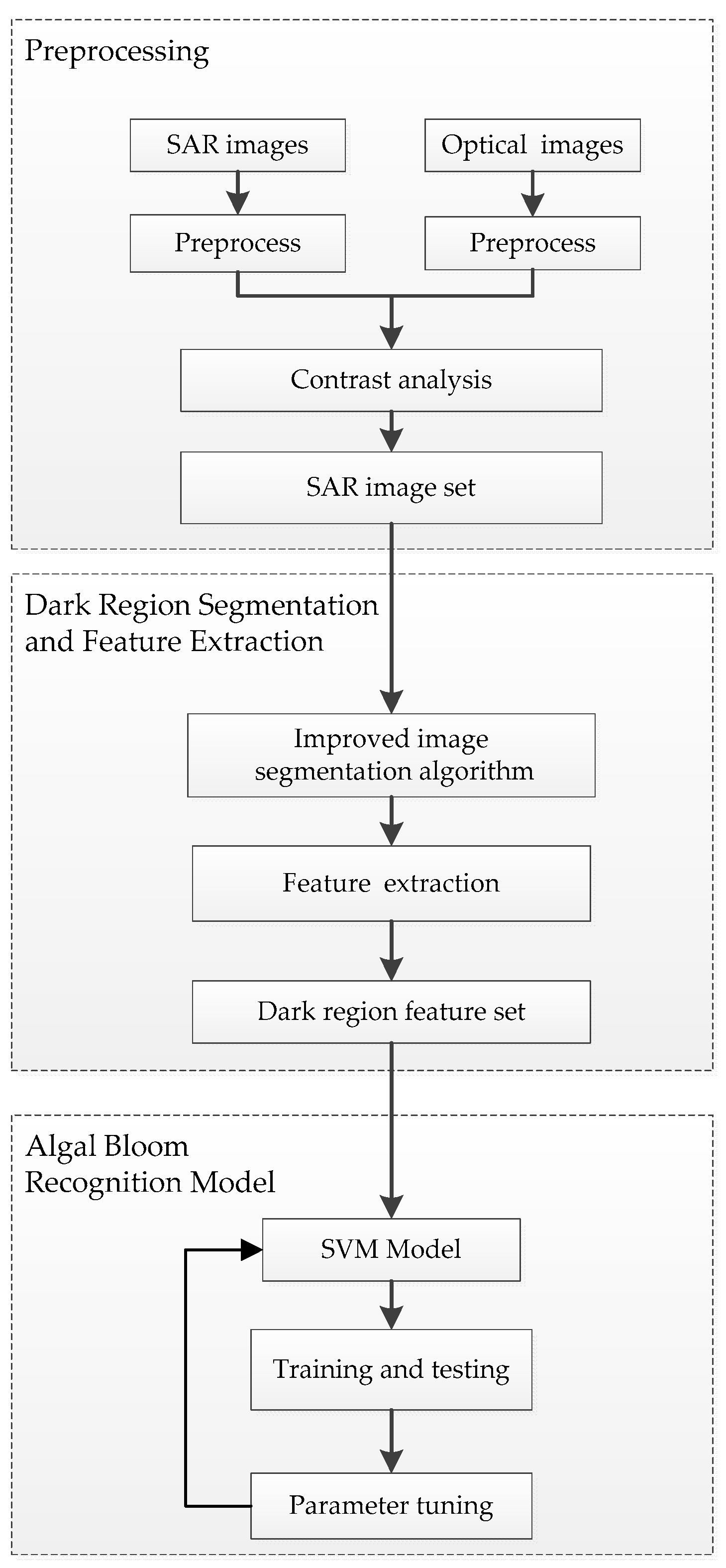
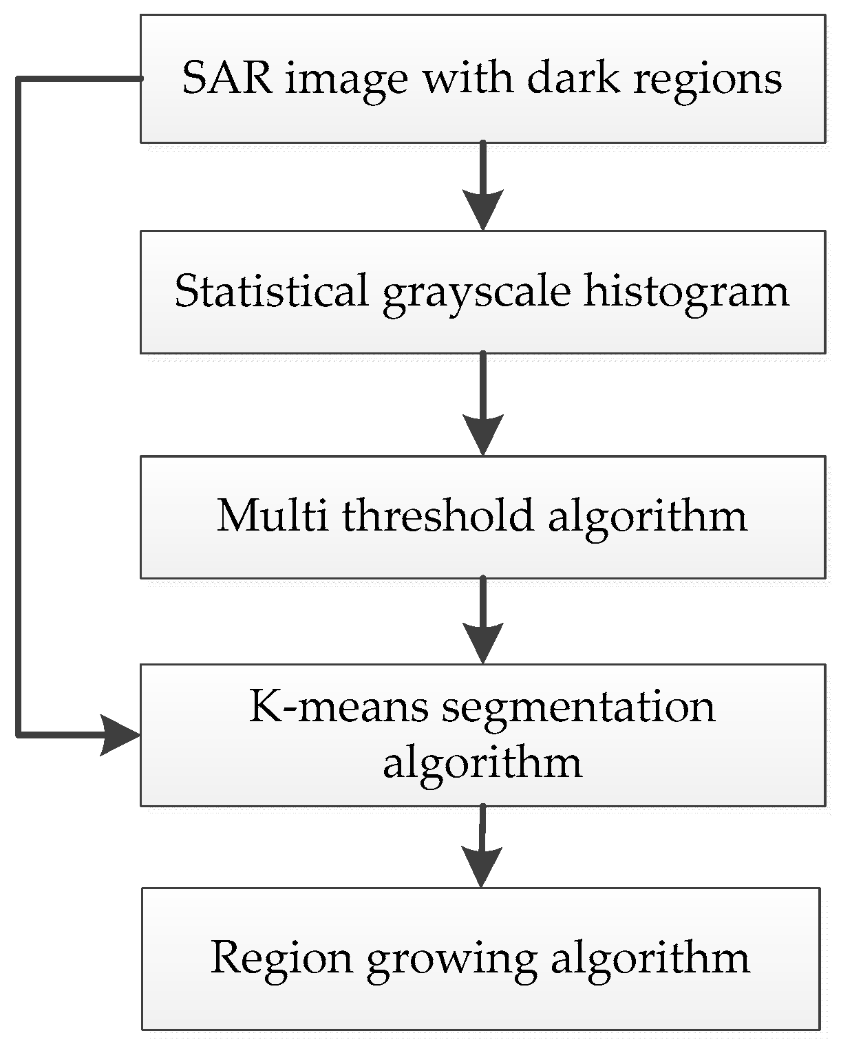
The flowchart of algal bloom recognition is shown in Figure 8. The purpose of preprocessing is to obtain the SAR image set, in which some dark regions are contained. During the preprocessing, the manual cropping of SAR images is adopted, by comparison with the quasi-synchronized optical images. When SAR images are segmented, some algorithms, including thresholding, clustering, and region growing, are applied. The feature extraction is executed to get the dark region features, including grayscale, geometry and texture. Based on the feature set, an algal bloom recognition model is developed, in which the support vector machine (SVM) is applied. A cross-validation method plays a role in the parameter tuning.
3.1. Dark Region Segmentation
The segmented results of the dark regions are directly related to the quality of the following feature extraction work. In this paper, a combination of multi-Otsu thresholding algorithm and K-means algorithm was applied to complete the segmentation of the dark regions.
3.1.1. Multi-Otsu Thresholding Algorithm
Otsu thresholding is one of the most commonly used methods to select a threshold for general images [40]. The main idea of the algorithm is to find the threshold that maximizes the between-class variance. An image can be described as . The average gray level of the entire image, , is computed as follows:
where is the number of distinct gray levels, represents one of the gray levels, represents the probability of occurrence of gray level , represents the number of pixels with gray level , and represents the total number of pixels in the gray image.
When a single threshold is used, the image is divided into two classes, and . consists of pixels with gray levels , and consists of pixels with gray levels .
The cumulative probabilities and the mean levels of and classes are calculated as follows:
where and represent the cumulative probabilities, and represent the mean levels.
For the threshold , the variance between two classes, is obtained as follows:
The optimal threshold of Otsu method can be determined as follows:
The multi-Otsu thresholding algorithm is determined based on the Otsu method. When an image is divided into classes, the different thresholds are used. The variance for different thresholds can be expressed as follows:
The optimal thresholds of the multi-Otsu thresholding algorithm can be determined as follows:
During the process of image segmentation, the multi-Otsu thresholding algorithm is used to find the optimal threshold in the global scope. However, some inherent imperfections limit its application. When the difference of the gray values between different categories is not obvious, or the gray ranges of different targets overlap, the segmentation effect of the global threshold will be poor, which may lead to inaccurate segmentation.
3.1.2. K-Means Segmentation Algorithm
K-means segmentation algorithm is an unsupervised machine learning method, which is characterized by high efficiency and simple implementation [41,42,43].
The main idea of the algorithm is given as follows:
- Input:
- The number of clusters and all data points, which are given as:where is a vector with dimensions, and N is the number of the data points.
- Output:
- Cluster centers and data points of clusters.
The steps are described as follows:
- Steps 1:
- Randomly select data points as the cluster centers .
- Steps 2:
- For each , assign it into the most relevant class , which is:
- Steps 3:
- Update the cluster centers , and the algorithm ends when the end condition is met, or it jumps to Steps 2.
In this algorithm, is a preset number. Additionally, the initial clustering centers of each class are selected randomly. The uncertainty of both k and the initial clustering centers will have a major impact on the results. The improper initial cluster may lead to convergence to local optimal value instead of the global one. At the same time the algorithm is sensitive to noise.
3.1.3. Integrated Algorithm of Dark Region Segmentation
To overcome the inadequacy of K-means algorithm, a combination of the multi-Otsu thresholding algorithm and K-means algorithm was adopted to improve k and the cluster centers. In addition, a region-growing algorithm was integrated to achieve better segmentation results.
On SAR images, the backscattering coefficient of the radar is represented by the gray levels. Grayscale histograms can visually distinguish the numbers and distribution of different grayscale values. The number of peaks represents the regional characteristics, and the number of valleys reflects the slowly varying characteristics. For grayscale statistical features, the fluctuation of grayscale should be identified. The number of the classes to be distinguished, can be expressed as:
where represents the number of peaks, represents the number of valleys.
Then the multi-Otsu thresholding segmentation algorithm is performed with segmentation thresholds, marked as . Using as the value of in the K-means algorithm, and the segmentation centers as the clustering centers, we can obtain:
The process of dark region segmentation is shown in Figure 9. The K-means algorithm is used to identify the local optimum value by calculating the minimum distance between each pixel and the clustering center, assigning the pixels to the nearest class, and then recalculating the mean of each class as the new clustering center. The number of categories was obtained by using the gray features of statistical images. The global optimal threshold , which is the clustering center of the K-means algorithm, was obtained by using the multi-Otsu thresholding algorithm. The clustering algorithm was used to initialize all classes to determine the maximum between-cluster variance. The threshold set, obtained by the multi-Otsu thresholding algorithm, is more representative than the randomly selected initial cluster centers.
The segmented image may have discontinuous areas, and small segmented regions may be significantly out of class. In this experiment, a self-selected center region growing algorithm was adopted, which means that a large image block was manually selected, and a connected domain with similar gray level attributes was segmented to form an area.
In this study, a total of 95 dark regions () were obtained by performing dark-region segmentation from 21 SAR images. Among them, 74 dark regions were found in 17 images of Taihu Lake, 14 dark regions were found in two images of Chaohu Lake, and seven dark regions were found in two images of Danjiangkou Reservoir. By comparing the quasi-synchronized optical images, it is found that 51 of all 95 dark regions represented algal bloom.
3.2. Feature Analysis and Extraction
3.2.1. Gray Features
As previously stated, SAR images include two types of dark region, which are algal bloom dark region and low-wind dark region, both of which presents the same or similar gray levels. However, a clear difference of the change of gray levels can be observed around the dark regions. The gray levels around the algal bloom dark regions show a transitional trend, while those around the low wind dark regions show a more moderate trend. Moreover, their mean and variance are also different.
The mean value of target area-to-background area ratio (MTBR), the mean to variance ratio of background (MVRB), and the gradient of edge (GOE) were selected as the gray level features for algal bloom recognition.
MTBR can be written as:
MVRB can be written as:
where represents mean and represents variance. The target and background region are selected by the segmentation algorithm mentioned above.
GOE is the gradient mean at the boundary of the target and the background region, and can be expressed as:
where and represent the horizontal and vertical gradients of the pixel , respectively, which can be calculated as:
where is the gray level of the pixel , and the size of the target image is pixels, is the Sobel operator, and represents the transposition of .
3.2.2. Geometrical Features
The spatial characteristics of algal bloom and low wind dark regions are different. Low wind dark regions in the lake present as large areas with a more regular shape. However, algal bloom dark regions, which often represent the strip distribution, are more dispersed because of the water flow. Based on these analyses, the parameters of area and complexity were selected as the geometric features for algal bloom recognition.
The area of dark region, S can be written as:
where is the number of pixel in the dark regions, and is the actual area of the pixel in dark regions.
Complexity (COM) reflects the shape feature of the target region, and can be written as:
where is obtained by Formula (21), and is the circumference of target region, which can be calculated by the “Regionprops” function in MATLAB.
3.2.3. Texture Features
Texture is an important feature of SAR images. Recognition accuracy of the bloom can be improved by combining different textural features. During the outbreak of algal bloom, the algae scum has a certain thickness and viscosity, which can smooth the water surface waves. The release of biosurfactants reduces the tension, dampens the capillary waves, and causes the dark region on water surface. As reflected in the image, the grayscale distribution of dark regions is relatively uniform. In general, the texture of algal bloom on a SAR image is delicate and smooth, while that of low wind dark regions is relative rough.
In this study, parameters including the angular second moment (ASM), contrast (CON), entropy (ENT), and the reciprocal difference moments (RDM) of the Gray-level co-occurrence matrix (GLCM) [44], commonly used to describe texture features, are selected for the algal bloom recognition.
ASM can be written as:
where i and j represent a gray value, represents a pixel with the gray value of i and the probability of being the gray value of j in the specified space distance and direction.
ASM is also known as energy. It represents the degree of distribution of gray levels in the image. A rougher texture corresponds to a larger ASM value. The energy caused by their “oily” property of algal bloom dark regions is smaller than that of low wind dark regions.
CON can be written as:
where represents the brightness of the image.
A greater difference between the local gray values corresponds to a greater contrast and a clearer visual effect. The CON of algal bloom dark regions is smaller, because it is smoother than low wind dark regions.
ENT can be written as:
where is an image measurement criterion.
The randomness of information directly affects the value of ENT. Therefore, a greater ENT value corresponds to a more complicated image. The ENT of algal bloom dark regions, which are smooth, is smaller than that of low wind dark regions.
RDM can be written as:
where represents the overall contrast of the image.
A greater value of RDM corresponds to a greater overall contrast.
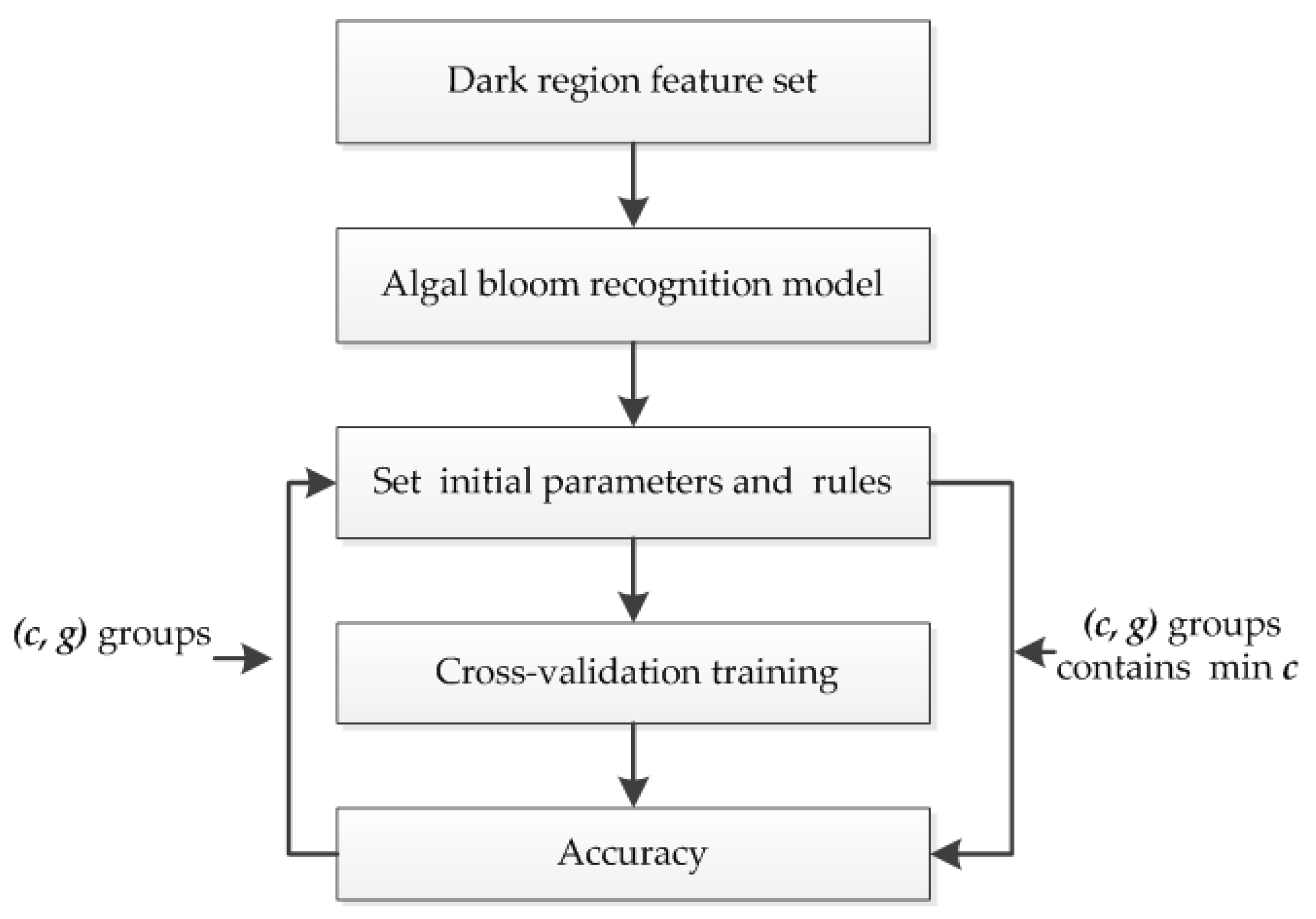
3.3. Algal Bloom Recognition Model
The SVM [45], which is based on statistical learning theory, is a machine learning method, and has been widely used in the field of remote sensing in recent years. The main idea of SVM is to find the optimal hyperplane to classify the input samples, where the gap between classes is guaranteed to be the largest. This optimal classifying hyperplane is described by the training samples. The generalization ability of SVM is based on the principle of minimized structural risk, and has the advantages of being able to quickly learn from small samples with high classification accuracy [46,47].
In this study, the radial basis function (RBF) is used in the C-SVM [48,49,50,51]. The algal bloom recognition model was optimized by the selected features of dark region sets.
The simplified model is stated as:
where is the data label that represents the class. It is assumed that two classes of data are expressed in [1, −1]. represents the parameter of RBF kernel. is the vector used to determine the gap between classes. represents the feature set extracted from all dark regions during the preceding process. , , and represent the feature set of gray, geometry, and texture, respectively. represents the penalty parameter.
In the model-building process, two parameters were used. The parameter determines the distribution of the data mapped to the new feature space. And the parameter represents the tolerance of error.
Parameter optimization greatly influences the recognition accuracy. The most commonly used method is taking values of and within a certain range, and then using cross-validation to find the optimal values of and which can make the recognition accuracy the highest.
During the parameter optimization, as shown in Figure 10, the minimum principle is used to select the set of and values. The smallest parameter is the best, which give rise to a higher recognition accuracy without reducing the generalizability of the model. As shown in Table 3, after optimizing the parameters, the accuracy of the recognition model tested on Taihu Lake is improved by four percentage points.
4. Results and Discussion
4.1. Results
4.1.1. Segmentation
In order to demonstrate the segmentation effect, three dark regions in the Taihu Lake and Chaohu Lake were selected as examples. Here, three different methods, which are traditional K-means algorithm, multi-Otsu thresholding method, and the segmentation algorithm proposed in this paper, were used to execute the segmentation. The results are shown in Figure 11.
To verify the effectiveness of the proposed method, the missing alarm rate (MA) and the false alarm rate (FA) were used. Furthermore, an assessment criterion noted as A was also introduced. The lower the values of MA and FA, the higher the accuracy of segmentation.
The corresponding calculation formulas can be written as:
where FN and TP represent the number of false and correct classification of dark region, FP and TN represent the number of false and correct classification of background, and P and N represent the total number of dark region and background, respectively.
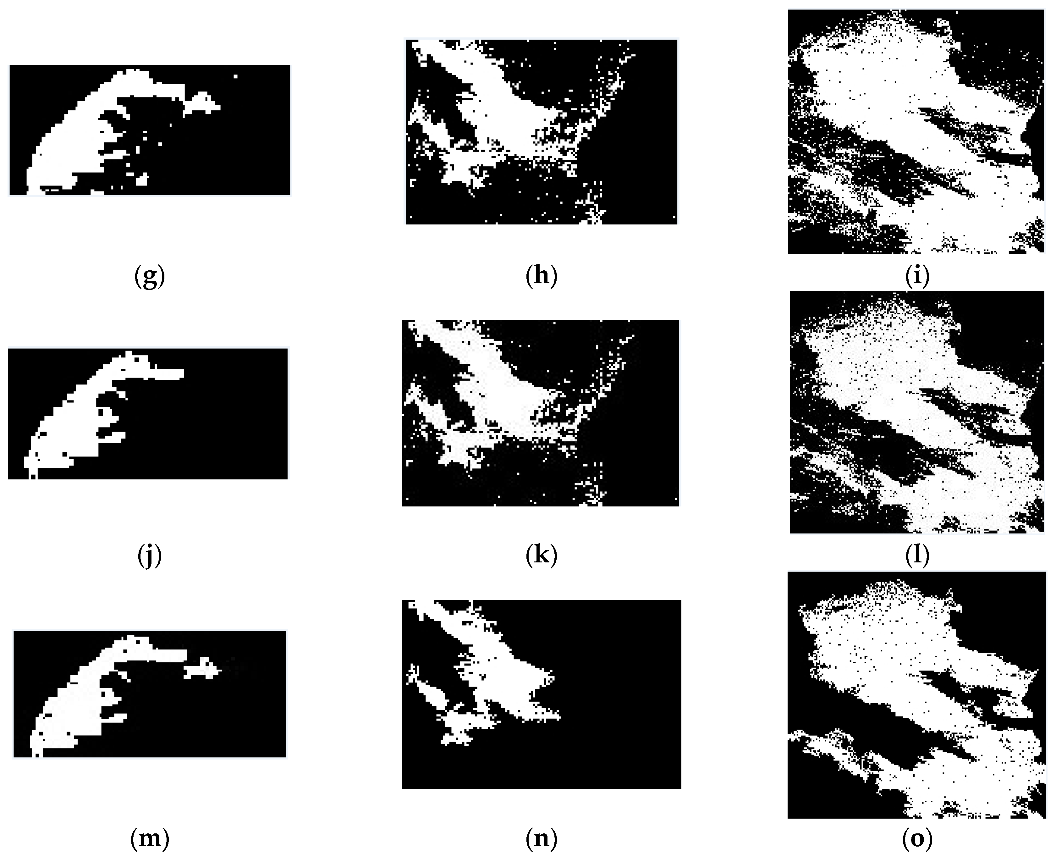
The accuracy of the segmentation algorithms of different regions was given in Table 4. The average accuracy of our algorithm is higher than the other two algorithms, with lower MA and FA at the same time. Therefore, our algorithm performs better at segmentation.
4.1.2. Recognition Model
In this experiment, the feature set of 74 dark regions extracted from the SAR images of Taihu Lake, was tested using the “leave-one-out” method. The dark regions on one image were used as the test data, and those on the other images were used to train the classifier. This procedure was repeated until all the images were tested.
A confusion matrix was used to evaluate the classification accuracy, shown as Table 5. The producer accuracies of the algal bloom and similar regions were 74.36% and 74.29%, respectively. The overall accuracy of all the dark regions was 74.00% in Taihu Lake, and the Kappa coefficient was 0.48. The Kappa coefficient was used for a consistency test [52]. A larger value of the Kappa coefficient represents a better result of classification.
Taking the Taihu Lake images as the training set, Chaohu Lake and Danjiangkou Reservoir were also tested in the same way. The results of accuracy analysis were given in Table 6. The overall accuracy was 71.00%, and the Kappa coefficient was 0.47. It can be seen from Table 6 that, when there was algal bloom, the recognition accuracy of the algal bloom dark regions reached 81.00%, but that of the non-algal bloom dark regions was relatively low.
As shown in Table 7, a total of 95 dark regions of Chaohu Lake, Danjiangkou Reservoir and Taihu Lake were classified and tested. The misclassified numbers of dark regions with different areas, was 5, 6, 13, respectively. Among the misclassified dark regions, 54.16% of them were larger than 20 km2, whereas the accuracy of the dark regions (<20 km2) was 83.00%. In view of this, it can be concluded that SAR can be used as an effective remote sensing tool for monitoring algal bloom in lakes.
4.2. Discussion
As reported in Table 5, the overall accuracy of the proposed method is 74.36%. By contrast, the accuracy in the Taihu Lake experiment, performed by Wang [23], who used ERS-2 and ENVISAT ASAR images, was 66.70%. Thus, our approach represents an improvement of eight percentage points. The subsequent experiments of Chaohu Lake and Danjiangkou Reservoir achieve an accuracy of 71.00%, indicating that the model can better monitor and identify algal bloom in the similar lakes.
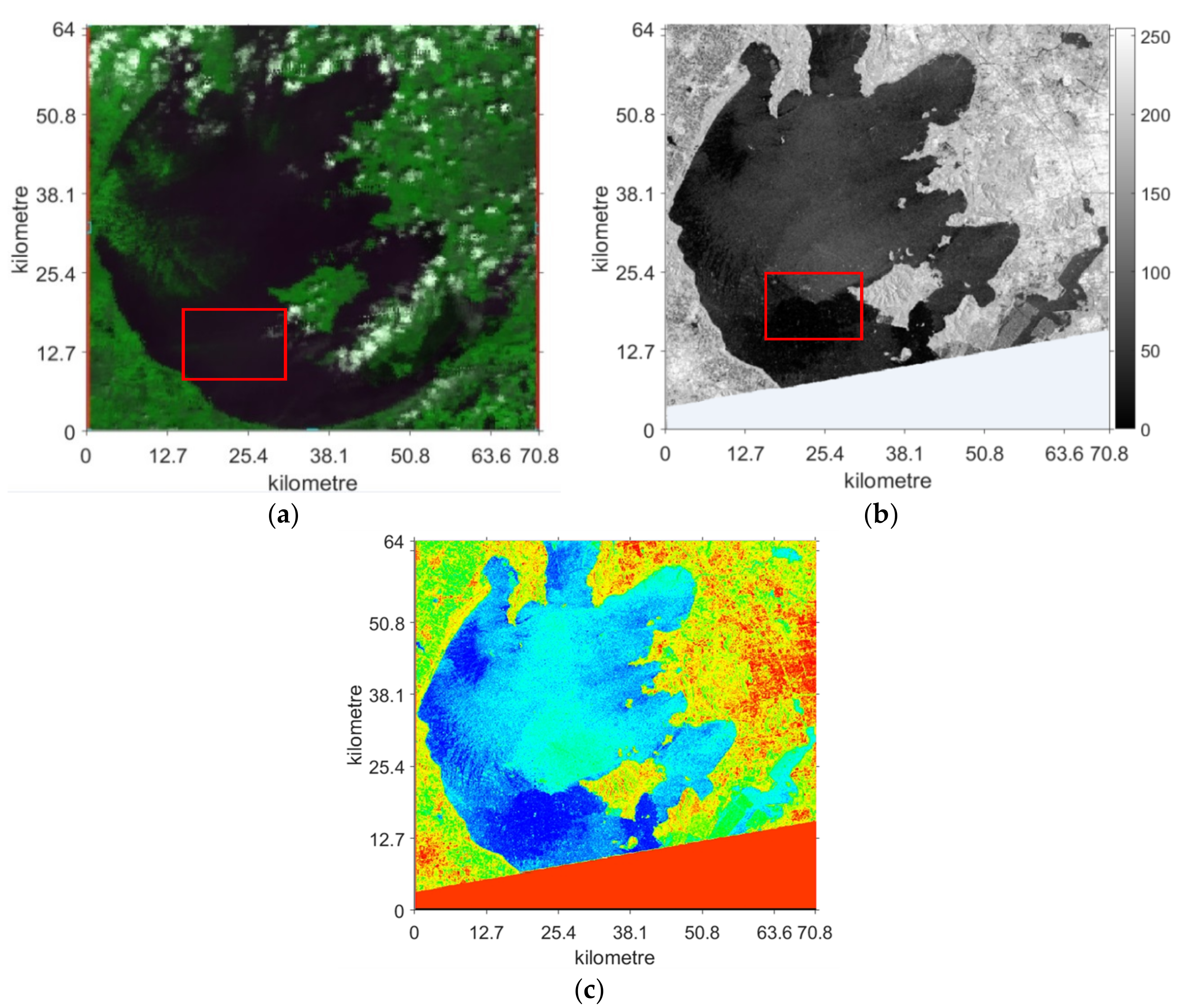
It is to be noted that some special cases can be observed, as shown in Figure 12. For example, the area of red frame in Figure 12a has a few green color, indicating the algal bloom trace. However, the dark regions in Figure 12b are larger, and extended to the western edge, which were different with those on the optical image. The time interval between the two images was 4.5 h. The weather information between 5:00 a.m. and 10:00 a.m. of that day was southeast wind, and the wind speed was smaller than a gentle breeze. At 10:00 a.m., the real-time wind speed in the southern lake was less than 1 m/s. Therefore, it can be inferred that the large dark region in Figure 12b was partly caused by the algal bloom, and the rest was due to other causes.
This in consistency reflects the limitation of using SAR images to recognize algal bloom. On the one hand, dark regions on water surface reflect the accumulation of algal bloom. On the other hand, low wind may also lead to dark region in SAR images. If the areas have both of the phenomena mentioned above, it would be difficult to recognize algal bloom. Introduction of quasi-synchronized optical images is a good solution to deal with this problem, and that is validated to be effective.
5. Conclusions
This study analyzed the ability to recognize algal bloom using SAR images, with the goal of replacing optical images in inadequate weather conditions. The algal bloom reduces the radar backscattering coefficient, and is presented as dark regions on SAR images. However, low wind shows as dark regions as well, which challenges with the application of SAR images. In this study, an algal bloom recognition model of SAR images was proposed, using the quasi-synchronized optical images, and the features of dark region. Some segmentation algorithms and C-SVM method were adopted in our model. According to the experimental results, the overall accuracy was 74.00% in Taihu Lake, and 71.00% in Chaohu Lake and Danjiangkou Reservoir. This tentative study shows the favorable application prospect of SAR monitoring. Moreover, the achievement of this study can be a supplementary means for algal bloom monitoring.
Although the accuracy of the algal bloom model proposed in this paper is higher, there are still several aspects to be improved. Firstly, the image set used is insufficient. If more images with different sensors and areas can be obtained, the results will be better. Secondly, more accurate and complete meteorological information, including temperature, wind speed, wind direction and so on, will help the improvement of recognition accuracy. Finally, the multi-band and multi-polarization SAR images, if available, can give more information of algal bloom on the water’s surface, which will be the examined in further studies in the future.
Author Contributions
L.W. and L.W. designed the study; L.W., L.M., Z.G., and J.Z. conducted the analysis and wrote the manuscript; and L.W., W.H. and N.L. contributed to discussions and revisions, providing important feedback and suggestions
Acknowledgments
All the authors are deeply grateful to the editors for their smooth and fast handling of the manuscript. The authors would also like to thank the anonymous referees for their valuable suggestions to improve the quality of this paper. This work is supported by the National Natural Science Foundation of China (Grant No. U1604145), the College Key Research Project of Henan Province (Grant No. 18B520010), and the Plan of Science and Technology of Henan Province (Grant No. 182102210233). The authors appreciate ESA’s free Sentinel-1A images and SNAP software.
Conflicts of Interest
The authors declare no conflict of interest.
References
- Smolowitz, R.; Shumway, S.E. Possible cytotoxic effects of the dinoflagellate, Gyrodinium aureolum, on juvenile bivalve molluscs. Aquac. Int. 1997, 5, 291–300. [Google Scholar] [CrossRef]
- Guo, L. Doing battle with the green monster of Taihu Lake. J. Sci. 2007, 317, 1166. [Google Scholar] [CrossRef] [PubMed]
- Oilver, R.I.; Ganf, G.G. Freshwater Blooms. In the Ecology of Cyanobacteria: Their Diversity in Time and Space; Whitton, B.A., Potts, M., Eds.; Kluwer: Dordrecht, The Netherlands, 2002; pp. 149–194. ISBN 978-0-7923-4735-4. [Google Scholar]
- Qin, B.Q.; Yang, G.J.; Ma, J.R.; Deng, J.M.; Li, W.; Wu, T.F.; Liu, L.Z.; Gao, G.; Zhu, G.W.; Zhang, Y.L. Dynamic characteristics and mechanism of “outbreak” of cyanobacteria bloom in Taihu. Sci. China Press 2016, 61, 759–770. [Google Scholar]
- Kong, F.X.; Hu, W.P.; Gu, X.H. On the cause of cyanophyta bloom and pollution in water intake area and emergency measures in Meiliang Bay, Lake Taihu in 2007. J. Lake Sci. 2007, 19, 357–358. [Google Scholar]
- Li, Y.; Shang, S.L.; Ma, X.X. Identification model of algal bloom based on the relationship between visible light and near infrared reflectance. J. Chin. Sci. Bull. 2005, 50, 2555–2561. [Google Scholar]
- Xu, J.P.; Zhang, B.; Li, F.; Song, K.S.; Wang, Z.M. Detecting modes of cyanobacteria bloom using MODIS data in Lake Taihu. J. Lake Sci. 2008, 20, 191–195. [Google Scholar]
- Ma, R.H.; Kong, W.J.; Duan, H.T.; Zhang, S.X. Quantitative estimation of phycocyanin concentration using MODIS imagery during the period of cynobacterial blooming in Taihu Lake. China Environ. Sci. 2009, 29, 254–260. [Google Scholar]
- Zhou, L.G.; Feng, X.Z.; Wang, C.H.; Wang, D.Y.; Xu, X.X. Monitoring cyanobacteria bloom based on MODIS data in Lake Taihu. J. Lake Sci. 2008, 20, 203–207. [Google Scholar]
- Jin, Y.; Zhang, Y.; Jiang, S. Application of EOS/MODIS Data for Research of Cyanobacteria Bloom Spatio- temporal Distribution in Taihu Lake. Environ. Sci. Technol. 2009, 22, 9–11. [Google Scholar]
- Lv, K. Remote Sensing Monitoring of Alage in Taihu Lake and its Early Warning. Master’s Thesis, University of Geosciences, Wuhan, China, 2015. [Google Scholar]
- Hu, C.M. A novel ocean color index to detect floating algae in the global oceans. Remote Sens. Environ. 2009, 113, 2118–2129. [Google Scholar] [CrossRef]
- Guo, W.C. Study on Extraction methods of cyanophytes bloom based on HJ-1. Master’s Thesis, Nanjing Normal University, Nanjing, China, 2011. [Google Scholar]
- Zhang, W.; Zhao, Y.L.; Xue, Y.; Liu, F.J. Research on the Spatial-Temporal Changes of Water Blooms in Dongting Lake Based on MODIS Data of 2000–2013 in China. Comput. Telecommun. 2014, 33–35. [Google Scholar] [CrossRef]
- Zhang, Y.J.; Wang, J.L.; Ran, Y.Y.; Yang, F.; Cao, X.M.; Guo, H.H. Estimating Chlorophyll-A Concentration in Poyang Lake using MODIS based on Measured Reflectance Spectra. Resour. Environ. Yangtze Basin 2013, 22, 1081–1089. [Google Scholar]
- Zhang, J.; Chen, L.Q.; Chen, X.L. Monitoring the cyanobacterial blooms based on remote sensing in Lake Erhai by FAI. J. Lake Sci. 2016, 28, 718–725. [Google Scholar] [CrossRef]
- Sun, H.; Xie, X.P. Monitoring of Enteromorpha prolifera and analysis of impact factors based on MODIS data in Rizhao offshore. Remote Sens. Land Resour. 2016, 28, 144–151. [Google Scholar] [CrossRef]
- Wang, G.L.; Li, J.S.; Zhang, B.; Cai, Z.Q.; Zhang, F.F.; Shen, Q. Synthetic aperture radar detection and characteristic analysis of cyanobacterial scum in Lake Taihu. J. Appl. Remote Sens. 2017, 11, 012006. [Google Scholar] [CrossRef]
- Sieburth, J.M.; Conover, J.T. Slicks associated with Trichodesmium Blooms in the Sargasso Sea. Nature 1965, 205, 830–831. [Google Scholar] [CrossRef]
- Alpers, W.; Wismann, V.; Theis, R.; Huhnerfuss, H.; Bartsch, N.; Moreira, J.; Lyden, J.D. The damping of ocean surface waves by monomolecular sea slicks measured by airborne multi-frequency radars during the SAXON-FPN experiment. Int. Geosci. Remote Sens. Symp. 2002, 4, 1987–1990. [Google Scholar]
- Gade, M.; Hühnerfuss, H.; Korenowski, G.M. (Eds.) On the Imaging of Biogenic and Anthropogenic Surface Films on the Sea by Radar Sensors; Springer: Berlin/Heidelberg, Germany, 2006; pp. 189–204. ISBN 3-540-33270-7. [Google Scholar]
- Wang, J.; Wang, S.X.; Yan, F.L.; Zhou, Q. Range Extraction of Alage Bloom Water Body on ASAR and MODIS. Remote Sens. Inf. 2009, 3, 54–57. [Google Scholar]
- Wang, G.L. Active and passive remote sensing of inland waters cyanobacteria bloom-Taking Taihu as an example. Master’s Thesis, East China Normal University, Shanghai, China, 2015. [Google Scholar]
- Bresciani, M.; Adamo, M.D.; Carolis, G. Monitoring blooms and surface accumulation of cyanobacteria in the Curonian Lagoon by combining MERIS and ASAR data. Remote Sens. Environ. 2014, 146, 124–135. [Google Scholar] [CrossRef]
- Yang, G.S.; Ma, R.H.; Zhang, L.; Jiang, J.H.; Yao, S.C.; Zhang, M.; Zeng, H.B. Lake status major problems and protection strategy in China. J. Lake Sci. 2010, 22, 799–810. [Google Scholar]
- Qin, B.Q.; Wang, X.D.; Tang, X.M.; Feng, S.; Zhang, Y.L. Drinking Water Crisis Caused by Eutrophication and Cyanobacterial Bloom in Lake Taihu: Cause and Measurement. J. Adv. Earth Sci. 2007, 22, 896–906. [Google Scholar]
- Ma, R.X.; Kong, F.X.; Duan, H.T.; Zhang, S.X.; Kong, W.J.; Hao, J.Y. Spatio-temporal distribution of cyanobacterial blooms based on satellite imageries in Lake Taihu, China. J. Lake Sci. 2008, 20, 687–694. [Google Scholar]
- Tan, X.; Xia, X.; Li, S. Water quality characteristics and integrated assessment based on multistep correlation analysis in the Danjiangkou reservoir, China. J. Environ. Inf. 2015, 25, 60–70. [Google Scholar] [CrossRef]
- Yang, J.; Wu, Z.R. Present Conditions and Development of Dam Safety Monitoring and Control Researches Home and Abroad. J. Xi’an Univ. Technol. 2002, 18, 26–30. [Google Scholar]
- Cheng, Q.L.; Zhu, T.Q. Water Environmental Assessment for the Danjiangkou Reservoir. Res. Soil Water Conserv. 2008, 15, 202–205. [Google Scholar]
- Li, S.Y.; Zhang, Q.F. Main Eco-Environmental Problems and Revegetation in the Danjiangkou Reservoir Water Supplying Area of the Middle Route of the South to North Water Transfer Project. China Rural Water Hydropower 2008, 3, 1–4. [Google Scholar]
- Kang, L.; Li, X.C. Risk analysis of synchronous asynchronous encounter probability of rich-poor precipitation in the Middle Route of South-to-North Water. J. Adv. Water Sci. 2011, 22, 44–50. [Google Scholar]
- Gu, X.C.; Fu, K.; Qiu, X.L. The Basis of Interpretation of SAR Image Interpretation; Zhang, H.N., Ed.; Science Press: Beijing, China, 2017; ISBN 9787030522979. [Google Scholar]
- Levkowitz, H.; Herman, G.T. Color scales for image data. IEEE Comput. Appl. 1992, 12, 72–80. [Google Scholar] [CrossRef]
- Li, Y.; Zhang, L.F.; Huang, C.P.; Wang, J.N.; Cen, Y. Monitor of Cyanobacteria Bloom in Lake Taihu from 2001 to 2013 Based on MODIS Temporal Spectral Data. Spectrosc. Spectr. Anal. 2016, 36, 1406–1411. [Google Scholar]
- Kong, F.X.; Gao, G. Hypothesis on cyanobacteria bloom-forming mechanism in large shallow eutrophic lakes. Acta Ecol. Sin. 2005, 25, 589–595. [Google Scholar]
- Kong, F.X.; Ma, R.H.; Gao, J.F.; Wu, X.D. The theory and practice of prevention, forecast and warning on cyanobacteria bloom in Lake Taihu. J. Lake Sci. 2009, 21, 314–328. [Google Scholar]
- Yang, Q.X. Algal bloom in Taihu Lake and it’s control. J. Lake Sci. 1996, 8, 67–74. [Google Scholar]
- Bai, X.H.; Hu, Z.X.; Li, X.H. Importation of Wind-Driven Drift of Mat-Like Algae Bloom into Meiliang Bay of Taihu Lake in 2004 Summer. Environ. Sci. 2005, 26, 57–60. [Google Scholar]
- Ohtsu, N. A threshold selection method from gray-level histograms. IEEE Trans. Syst. Man Cybern. 1979, 9, 62–66. [Google Scholar] [CrossRef]
- Patel, B.C.; Sinha, D.G.R. An adaptive K-means clustering algorithm for breast image segmentation. Int. J. Comput. Appl. 2010, 10, 35–38. [Google Scholar] [CrossRef]
- Ma, G.Q.; Wang, X.J. An Efficient Algorithm Optimization of CT Images Segmentation Based on K-Means Clustering. Appl. Mech. Mater. 2014, 530, 386–389. [Google Scholar] [CrossRef]
- Isa, N.M.; Salamah, S.A.; Ngah, U.K. Adaptive fuzzy moving K-means clustering algorithm for image segmentation. J. Consumer Electron. IEEE Trans. 2009, 55, 2145–2153. [Google Scholar]
- Gao, C.C.; Hui, X.W. GLCM-based texture feature extraction. Comput. Syst. Appl. 2010, 19, 195–198. [Google Scholar]
- Peng, L. Research on Classification Algorithm of Support Vector Machine and It Application. Master’s Thesis, Hunan University, Changsha, China, 2007. [Google Scholar]
- Vapnik, V.N. The Nature of Statistical Learning Theory; Springer: New York, NY, USA, 1995; ISBN 9780387987804. [Google Scholar]
- Vapnik, V.N. Statistical Learning Theory; Wiley-Interscience Wiley: New York, NY, USA, 1998; ISBN 9780471030034. [Google Scholar]
- Burges, C.J.C. A tutorial on support vector machines for pattern recognition. Data Min. Knowl. Discov. 1998, 2, 121–167. [Google Scholar] [CrossRef]
- Ma, J.S.; Berg, A.C.; Malik, J. Classification using intersection kernel support vector machines is efficient. Comput. Vis. Pattern Recogn. J. IEEE 2008, 21, 1–8. [Google Scholar]
- Scholkopf, B.; Sung, K.B.C. Comparing support vector machines with Gaussian kernels to radial basis function classifiers. J. Signal Process. 1997, 45, 2758–2765. [Google Scholar] [CrossRef]
- Weston, J.; Watkins, C. Multiclass Support Vector Machines; Springer: London, UK, 2005; Volume 102, pp. 83–128. [Google Scholar]
- Cohen, J.A. coefficient agreement for nominal data. Educ. Psychol. Meas. 1960, 2, 37–46. [Google Scholar] [CrossRef]
Figure 1.
Study areas, including Danjiangkou Reservoir, Taihu Lake, and Chaohu Lake.

Figure 2.
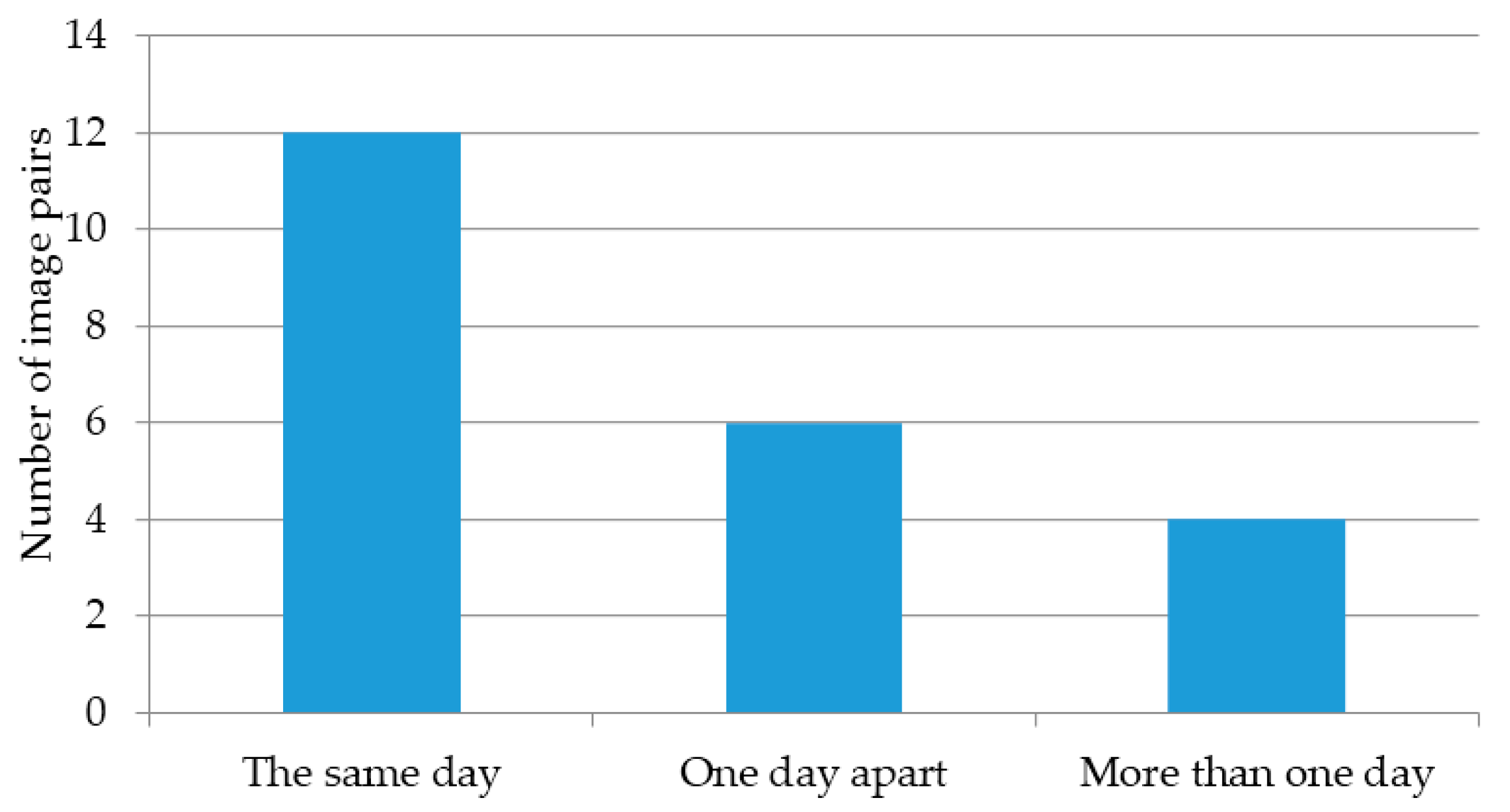
Statistical results of the time lags between optical and SAR images.

Figure 3.
Procedures of Sentinel-1A image preprocessing.

Figure 4.
Preprocessed images of Taihu Lake: (a) acquired SAR image from Sentinel-1A on 25 July 2015; (b) false color image of (a); (c) acquired optical image from Landsat-8 on 27 July 2015; and (d) acquired optical image from MODIS on 11 September 2015.
Figure 4.
Preprocessed images of Taihu Lake: (a) acquired SAR image from Sentinel-1A on 25 July 2015; (b) false color image of (a); (c) acquired optical image from Landsat-8 on 27 July 2015; and (d) acquired optical image from MODIS on 11 September 2015.

Figure 5.
Different eutrophication areas of Taihu Lake.

Figure 6.
A pair of optical and SAR images of Taihu Lake: (a) Acquired Landsat-8 image on 11 September 2015; (b) acquired Sentinel-1A image on 11 September 2015; and (c) false color image of (b).
Figure 6.
A pair of optical and SAR images of Taihu Lake: (a) Acquired Landsat-8 image on 11 September 2015; (b) acquired Sentinel-1A image on 11 September 2015; and (c) false color image of (b).


Figure 7.
The zoomed area of Figure 6: (a,b) the zoomed image of region ① in Figure 6a,b, respectively. (c,d) region ②. (e,f) region ③. (g,h) region ④. (i,j) region ⑤.


Figure 8.
Flowchart of algal bloom recognition.

Figure 9.
Flowchart of dark region segmentation.

Figure 10.
Flowchart of parameter optimization.

Figure 11.
Dark region segmentation results: (a,b) are manually cropped dark regions of Taihu Lake SAR image; (c) is that of Chaohu Lake SAR image; (d–f) are the segmented dark regions of (a–c); (g–i) are obtained by the traditional K-means algorithm; (j–l) are obtained by the multi-Otsu thresholding algorithm; (m–o) are obtained by the method proposed in this paper.


Figure 12.
The optical and SAR images after cropping: (a) acquired MODIS image at 5:35 UTC on 12 September 2017; (b) acquired SAR image at 10:00 UTC on 12 September 2017; and (c) false color image of (b).
Figure 12.
The optical and SAR images after cropping: (a) acquired MODIS image at 5:35 UTC on 12 September 2017; (b) acquired SAR image at 10:00 UTC on 12 September 2017; and (c) false color image of (b).


Table 1.
Acquired SAR images used in this study.
| Area | Acquired Image Date |
|---|---|
| Taihu Lake | 2 May 2015, 21 May 2015, 18 August 2015, 11 September 2015, 5 October 2015, 14 July 2016, 26 July 2016, 7 August 2016, 17 September 2016, 24 October 2016, 7 August 2017, 19 August 2017, 31 August 2017, 12 September 2017, 24 September 2017, 6 October 2017, 30 October 2017 |
| Chaohu Lake | 11 August 2015, 16 September 2015,21 December 2015 |
| Danjiangkou Reservoir | 24 December 2015, 20 August 2016, 31 October 2016 |
Table 2.
Acquired optical images used in this study.
| Area | Acquired Image Date |
|---|---|
| Taihu Lake | 1 May 2015, 3 May 2015, 21 May 2015, 17 August 2015, 19 August 2015, 11 September 2015, 15 July 2016, 26 July 2016, 7 August 2016, 18 September 2016, 6 August 2017, 19 August 2017, 12 September 2017, 26 September 2017, 7 October 2017, 30 October 2017 |
| Chaohu Lake | 16 September 2015, 21 December 2015 |
| Danjiangkou Reservoir | 24 December 2015, 20 August 2016, 31 October 2016 |
Table 3.
Accuracy of the recognition model tested on Taihu Lake.
| Initial | After Optimization | |
|---|---|---|
| Parameters | g = 1; c = 1 | g = 1.74; c = 0.0039063 |
| Accuracy | 0.70 | 0.74 |
Table 4.
Accuracy of the segmentation algorithms.
| Dark Regions | Algorithm | Accuracy | Missing Alarm Rate | False Alarm Rate |
|---|---|---|---|---|
| Figure 11a | Multi-Otsu thresholding | 95.00% | 0.1685 | 0.0098 |
| K-means | 96.00% | 0.0562 | 0.097 | |
| Our algorithm | 97.00% | 0.1205 | 0.0287 | |
| Figure 11b | Multi-Otsu thresholding | 92.00% | 0.0452 | 0.2881 |
| K-means | 89.00% | 0.0348 | 0.3345 | |
| Our algorithm | 97.00% | 0.1217 | 0.0548 | |
| Figure 11c | Multi-Otsu thresholding | 89.00% | 0.1100 | 0.0748 |
| K-means | 89.00% | 0.0546 | 0.1368 | |
| Our algorithm | 93.00% | 0.0995 | 0.0419 |
Table 5.
Confusion matrix for recognizing the dark regions of Taihu Lake.
| Blooms | Similar to Blooms | Accuracy | Overall Accuracy | Kappa Coefficient | |
|---|---|---|---|---|---|
| Blooms | 29 | 9 | 76.31% | ||
| Similar to blooms | 10 | 26 | 72.22% | 0.74 | 0.48 |
| Accuracy | 74.36% | 74.29% |
Table 6.
Confusion matrix for recognizing the dark regions of Danjiangkou Reservoir and Chaohu Lake.
Table 6.
Confusion matrix for recognizing the dark regions of Danjiangkou Reservoir and Chaohu Lake.
| Blooms | Similar to Blooms | Accuracy | Overall Accuracy | Kappa Coefficient | |
|---|---|---|---|---|---|
| Blooms | 9 | 3 | 75.00% | ||
| Similar to blooms | 2 | 6 | 75.00% | 0.71 | 0.47 |
| Accuracy | 81.81% | 67.67% |
Table 7.
Misclassified numbers of dark regions.
| Area (km2) | |||
|---|---|---|---|
| 1–10 | 10–20 | >20 | |
| Misclassified | 5 | 6 | 13 |
| Total | 32 | 30 | 33 |
© 2018 by the authors. Licensee MDPI, Basel, Switzerland. This article is an open access article distributed under the terms and conditions of the Creative Commons Attribution (CC BY) license (http://creativecommons.org/licenses/by/4.0/).
Share and Cite
MDPI and ACS Style
Wu, L.; Wang, L.; Min, L.; Hou, W.; Guo, Z.; Zhao, J.; Li, N. Discrimination of Algal-Bloom Using Spaceborne SAR Observations of Great Lakes in China. Remote Sens. 2018, 10, 767. https://doi.org/10.3390/rs10050767
AMA Style
Wu L, Wang L, Min L, Hou W, Guo Z, Zhao J, Li N. Discrimination of Algal-Bloom Using Spaceborne SAR Observations of Great Lakes in China. Remote Sensing. 2018; 10(5):767. https://doi.org/10.3390/rs10050767
Chicago/Turabian StyleWu, Lin, Le Wang, Lin Min, Wei Hou, Zhengwei Guo, Jianhui Zhao, and Ning Li. 2018. "Discrimination of Algal-Bloom Using Spaceborne SAR Observations of Great Lakes in China" Remote Sensing 10, no. 5: 767. https://doi.org/10.3390/rs10050767
Note that from the first issue of 2016, this journal uses article numbers instead of page numbers. See further details here.