Daily Retrieval of NDVI and LAI at 3 m Resolution via the Fusion of CubeSat, Landsat, and MODIS Data


1
Geospatial Sciences Center of Excellence, South Dakota State University, Brookings, SD 57007, USA
2
Department of Geography, South Dakota State University, Brookings, SD 57007, USA
3
Water Desalination and Reuse Center, King Abdullah University of Science of Technology, Thuwal 23955, Saudi Arabia
*
Author to whom correspondence should be addressed.
Remote Sens. 2018, 10(6), 890; https://doi.org/10.3390/rs10060890
Submission received: 18 March 2018
/
Revised: 23 May 2018
/
Accepted: 5 June 2018
/
Published: 7 June 2018
(This article belongs to the Special Issue Multisource Remote Sensing Data Fusion and Applications in Vegetation Monitoring)
Abstract
:Constellations of CubeSats are emerging as a novel observational resource with the potential to overcome the spatiotemporal constraints of conventional single-sensor satellite missions. With a constellation of more than 170 active CubeSats, Planet has realized daily global imaging in the RGB and near-infrared (NIR) at ~3 m resolution. While superior in terms of spatiotemporal resolution, the radiometric quality is not equivalent to that of larger conventional satellites. Variations in orbital configuration and sensor-specific spectral response functions represent an additional limitation. Here, we exploit a Cubesat Enabled Spatio-Temporal Enhancement Method (CESTEM) to optimize the utility and quality of very high-resolution CubeSat imaging. CESTEM represents a multipurpose data-driven scheme for radiometric normalization, phenology reconstruction, and spatiotemporal enhancement of biophysical properties via synergistic use of CubeSat, Landsat 8, and MODIS observations. Phenological reconstruction, based on original CubeSat Normalized Difference Vegetation Index (NDVI) data derived from top of atmosphere or surface reflectances, is shown to be susceptible to large uncertainties. In comparison, a CESTEM-corrected NDVI time series is able to clearly resolve several consecutive multicut alfalfa growing seasons over a six-month period, in addition to providing precise timing of key phenological transitions. CESTEM adopts a random forest machine-learning approach for producing Landsat-consistent leaf area index (LAI) at the CubeSat scale with a relative mean absolute difference on the order of 4–6%. The CubeSat-based LAI estimates highlight the spatial resolution advantage and capability to provide temporally consistent and time-critical insights into within-field vegetation dynamics, the rate of vegetation green-up, and the timing of harvesting events that are otherwise missed by 8- to 16-day Landsat imagery.
1. Introduction
Satellite remote sensing offers unparalleled opportunities for land surface monitoring and characterization over space and time domains, with far-reaching socioeconomic benefits [1,2,3]. Growing global food security concerns [4] necessitate space-borne observing systems that provide time-critical sensing of agricultural systems together with actionable intelligence for optimizing sustainable management practices, agricultural efficiencies, and crop production [5,6,7]. In the context of precision agriculture, timely and repeatable information on intrafield variability of crop conditions is key to achieving sustainable resource allocation and utilization [8,9]. Similarly, agricultural management decisions (e.g., timing of irrigation, fertilizer application, and harvesting) could benefit tremendously from continuous and near real-time observations of crop phenological development [10,11].
Space-borne observing capacity has evolved significantly in terms of spectral, spatial, and temporal resolution since the launch of the first Land Remote Sensing Satellite (Landsat) in 1972 [12,13]. However, the inevitable trade-off between resolvable spatial detail and frequency of observations [14] continues to affect the capacity to rapidly detect evolving vegetation dynamics at spatial scales fine enough for effective resource management. These spatiotemporal restrictions have been partly overcome via multisensor data fusion algorithms designed to synergistically exploit sensor-specific attributes, such as the high spatial resolution (i.e., 30 m) of Landsat and high revisit frequency (i.e., daily) of MODIS [15]. As an example, the spatial and temporal adaptive reflectance fusion model (STARFM) [16] has been used to predict surface reflectance [17,18], leaf area index [19], land surface temperature [20], and evapotranspiration [21,22] at both high spatial and temporal resolution. However, the lack of actual observations to inform upon intrinsic (i.e., at the scale of interest) spatial features at the time of prediction can introduce uncertainties that may affect the ability to meet often stringent product accuracy criteria [23]. Additionally, the conditional requirement of a sufficient number of homogeneous pixel samples at the coarse scale may not be met over heterogeneous landscapes associated with a relatively small characteristic field size [16].
The recent deployment of two identical Sentinel-2 satellites [24] represents an important advance towards resolving the classical spatiotemporal divide. The combination of high spatial resolution (<30 m) Landsat 8 and Sentinel-2 observations can facilitate a global median average revisit interval of about three days [25], which highlights the key importance of multisensor integration and interproduct harmonization efforts [26,27]. However, the achievable frequency is still suboptimal for detecting rapid vegetation dynamics and the exact timing of abrupt change events, particularly in light of obfuscating atmospheric effects (e.g., clouds, dust) which limit visibility and reduce the achievable repeat rate. While daily imaging at very high spatial resolution (<5 m) may be facilitated by commercial operators of programmable sensor constellations (e.g., WorldView, Pleiades), the satellite tasking is area-limited and prohibitively expensive [12].
One solution may lie in the cost-effective observation strategy offered by emerging constellations of small satellites, which is on a fast-track to revolutionize the earth observation potential [14]. This new operational paradigm has been facilitated by the standardized CubeSat concept [28] that uses compact and light-weight (<1.33 kg) single-unit (1U; 10 × 10 × 11.35 cm) building blocks as the modular basis for forming larger satellite configurations (i.e., 3U, 6U, 12U) for a variety of application fields [29]. As CubeSats are comprised largely of commercial off-the-shelf components and deployed as secondary payload on reusable rockets, the changing economics of earth observation have made it feasible to launch CubeSats in flocks at an unprecedented rate [30]. Planet [31] is leading the way in exploiting this new resource and its constellation of 3U CubeSats deployed in low-earth orbits has realized daily global imaging over terrestrial surfaces with an orthorectified pixel size of 3.125 m.
The number of explorative investigations into the potential benefits afforded by CubeSat data for land surface characterization is still limited and based on relatively short and temporally sparse records available at the time of study. The opportunities of CubeSat detectable intrafield-scale NDVI variability for precision agriculture were first demonstrated by Houborg and McCabe [32], while McCabe et al. [30] showcased their potential for providing valuable temporal insights into vegetation dynamics and evaporation. However, the relatively inexpensive and less advanced sensor designs do not come without limitations. Spectral bandwidth and response limitations, together with low radiometric quality relative to rigorously calibrated conventional satellites (e.g., Landsat and Sentinel), result in cross-sensor inconsistencies, which can severely affect the interpretability and utility of CubeSat-based time series records [33]. The Cubesat Enabled Spatio-Temporal Enhancement Method (CESTEM) was designed to optimize the benefit afforded by CubeSats via radiometric normalization against Landsat 8 observations [33]. Application of CESTEM to a limited time series of CubeSat imagery demonstrated accurate reproduction of Landsat-consistent surface reflectances at the scale and frequency of CubeSat observations, highlighting potentially far reaching implications via high quality, timely, and temporally consistent sensing at subfield scales [33].
In this study, we demonstrate an expanded application of CESTEM to a temporally dense record of CubeSat scenes acquired over an agricultural farming area in Saudi Arabia. Key advancements include an improved technique for smooth phenology reconstruction and an extension to map Landsat-based leaf area index (LAI) at the spatial and temporal resolution of the CubeSat data (i.e., CESTEM-LAI). The overall objective is to demonstrate the potential of the +170 CubeSat constellation for producing Landsat-consistent vegetation metrics at the highest spatiotemporal resolution ever retrieved from space-based sensors. The specific objectives of the study are: (1) to evaluate and intercompare the robustness and consistency of NDVI time series derived from “raw” and CESTEM-corrected CubeSat data over a highly dynamic multicut alfalfa field; and (2) to demonstrate and evaluate the capacity of the CESTEM framework for spatiotemporal enhancement of Landsat-based LAI.
2. Materials and Methods
This study used CubeSat (Section 2.1), Landsat 8 (Section 2.2), and MODIS (Section 2.3) data acquired over an irrigated farming area (~2400 ha) in Saudi Arabia (Figure 1) over a six-month period from 24 April to 25 October 2017. Alfalfa and corn were the predominant crops under pivot (~800 m in diameter) irrigation during this period. While the corn cultivated at the farm is characterized by two distinct growing seasons, with planting dates in the spring and the fall, alfalfa is grown continuously as a multicut crop with a 30–40 day harvesting frequency [34]. During this time, the average daytime air temperature high varied from ~45 °C during the summer months to ~35 °C in October. Sky conditions were predominantly free of clouds although prone to occasionally high dust aerosol loadings [35].
2.1. CubeSats
CubeSat data were acquired from the PlanetScope (PS) constellation that is commercially operated by Planet [31]. The constellation currently consists of >170 active 3U (i.e., 10 × 10 × 30 cm) CubeSats (“Doves”). At the time of writing, the PS constellation is capturing daily RGB and near-infrared (NIR) imaging of the earth’s terrestrial surfaces with a 3–4 m ground sampling distance (GSD). The vast majority of the CubeSats are deployed into sun-synchronous orbits (~475 km orbit altitude) with a midmorning equatorial overpass time (9:30–11:30 a.m., local solar time) and a nadir GSD between 3.5–4 m. Smaller flocks of PS satellites still operate in the International Space Station orbit (400 km altitude), which results in a variable equatorial overpass time and a GSD of ~3 m. Each CubeSat is associated with unique spectral response functions, and in addition to being significantly broader than the discrete bands of Landsat 8, the bands in the visible domains are characterized by substantial overlap [33].
Here, we used the Level 3A PlanetScope Ortho Tile Product that merges a consecutive series of individual scenes (typically four to five) from a single satellite into 25 × 25 km tiles referenced to a UTM map projection and with an orthorectified pixel size of 3.125 m [33,36]. The products have been geometrically corrected with a positional accuracy typically better than 10 m root-mean-square-error. Planet recently implemented a fairly rigorous radiometric correction approach based on a combination of prelaunch calibration, lunar calibration, and on-orbit cross-sensor calibration based on crossovers with rigorously calibrated sensor systems such as RapidEye and Landsat 8. The updated calibration approach has been verified against a limited number of vicarious collections (i.e., 12 samples covering a narrow reflectance range) over the Railroad Valley desert site in Nevada, which suggested a radiometric accuracy within ±10% of the top of atmosphere (TOA) reflectance reference and an average constellation uncertainty on the order of 5–6% [36,37]. This suggests a significant improvement over the first generations of Planet CubeSats [32,33].
The Planet data were converted to TOA reflectance using the calibration coefficients associated with each scene. In order to investigate the impacts of atmospheric effects, conversion of the at-sensor radiance to surface reflectance was undertaken using the Second Simulation of the Satellite Signal in the Solar Spectrum (6SV) atmospheric correction approach using sensor-specific spectral response functions, scene-specific view and illumination geometry, and satellite-based atmospheric state data (Section 2.2).
2.2. Landsat 8
Landsat 8 (L8) data were acquired over the study region with an 8–16-day revisit period using data from overlapping 165/43 and 164/43 path/row acquisitions. Whereas the 165/43 acquisitions provide full farm coverage, the 164/43 scene swath edge is positioned on the western half of the farm, with the exact location dependent on the day of the overpass. As a result, the study region is divided into sections with an 8-day, 8–16-day, and 16-day repeat coverage (Figure 1). L8 is positioned in a sun synchronous orbit (~705 km orbit altitude) with an equatorial overpass time between 9:56 a.m. and 10:26 a.m. (local solar time). The Operational Land Imager (OLI) surveys the earth in a 185-km swath (with a maximum view angle of ±7.5°) acquiring data in nine spectral bands distributed over the visible to near-infrared (VNIR) and shortwave-infrared domain. However, only the blue (band 2), green (band 3), red (band 4), and NIR (band 5) bands were considered here. The radiometric reflectance accuracy of the OLI is generally within the 3% sensor design specifications, supported by extensive vicarious calibration campaigns [23]. The Level-1 Terrain and Precision (L1TP) corrected dataset [38] was used in this study.
At-sensor radiance was converted into surface reflectance using an implementation of the 6SV [39,40], specifically adapted to handle the impacts of dust aerosols and adjacency effects over desert environments [23]. Inputs to 6SV include scene-specific sun-sensor geometry, total ozone from the Ozone Monitoring Instrument (OMI), atmospheric profiles of water and temperature from the Atmospheric Infrared Sounder (AIRS), and aerosol optical thickness at 550 nm (AOT550) from MODIS deep blue algorithm retrievals [23]. Further details on the atmospheric correction approach can be found in Houborg and McCabe [23,41].
Landsat-based leaf area index (LAI) was mapped over the study domain using prediction models previously developed over the study site on the basis of a hybrid machine-learning approach [41]. The technique utilizes an implementation [42] of the Cubist rule-based regression tree approach [43,44,45] to define the relationship between a suite of atmospherically corrected L8 vegetation indices (VI) and the target property (i.e., LAI). In Cubist, each terminal node of the learned tree is associated with a multivariate linear regression model and defined by a set of spectral threshold conditions (i.e., rules). A multiday hybrid LAI target training dataset was used, consisting of in situ measurements coupled with physically based retrievals independently derived via an implementation of the regularized canopy reflectance model (REGFLEC) [46]. The addition of REGFLEC-based LAI targets significantly improved model predictability and portability, yielding a cross-validated relative mean absolute difference (rMAD) of ~11% relative to an rMAD of ~18% for the in situ only training case. The optimal LAI prediction model was formulated as two multivariate regression equations combining VIs derived from visible, near-infrared, and shortwave-infrared L8 bands (see Equations (1a) and (1b) in Houborg and McCabe [41]). Interestingly, models relying only on standard indices formed from red and NIR band reflectances (e.g., NDVI) were associated with a substantially higher retrieval uncertainty (i.e., rMAD ~ 21%).
2.3. MODIS
MODIS surface reflectance data were acquired on days coincident with CubeSat acquisitions. The version 6 combined (i.e., Terra and Aqua) MCD43A4 product [47] was used, which provides daily 500 m surface reflectances in seven bands normalized to a nadir view direction and local solar noon using a semiempirical bidirectional reflectance distribution function (BRDF) [48]. The data are provided in a sinusoidal projection grid on 1200 × 1200 km tiles. Only the four bands in the VNIR were retained for further analyses. MODIS has a wide field of view (±55°) and corrections for reflectance anisotropy are generally needed to produce temporally consistent time-series data. The BRDF utilizes the best observations from both Terra and Aqua sensors collected over a 16-day period centered on the day of interest. Observations at the day of interest are emphasized in the daily retrievals. The associated quality flags were used to isolate high-quality retrievals that have an accuracy of ~5% [49].
2.4. CESTEM
This section describes the framework of the CubeSat Enabled Spatio-Temporal Enhancement Method (CESTEM) [33], including an extension (CESTEM-LAI) that maps LAI to the spatial and temporal resolution of the CubeSat data (Figure 2). At its core, CESTEM serves as a radiometric normalization technique to translate broadband (RGB + NIR) PS data acquired from multiple CubeSats into L8-consistent surface reflectances (i.e., blue, green, red, and NIR). The approach relies on the availability of L8 reference data on the CubeSat prediction day (Pday) to learn band-specific translational associations on a scene-specific basis using the Cubist decision tree regression approach, as detailed in Houborg and McCabe [33]. L8 reference data are drawn from the available pool of Landsat images, using MODIS-based information to quantify spectral changes over given CubeSat–Landsat acquisition timespans (Section 2.4.2). CESTEM-LAI (Section 2.4.4) uses the normalized L8-consistent PS data together with L8-based reference LAI in a similar fashion to generate maps of LAI at the spatial and temporal resolution of the CubeSat data. All of these processes have been designed for complete automation. A detailed description of the generic methodology and processing steps schematized in Figure 2 is provided in subsequent sections.
2.4.1. Data Preprocessing
PlanetScope Ortho Tile Product (Section 2.1), L8 L1TP (Section 2.2), and MODIS MCD43A4 (Section 2.3) images are acquired programmatically using Planet’s API, Google Cloud Platform, and the data pool portion of the Land Processes Distributed Active Archive Center (LP DAAC), respectively. In the case of PS acquisitions, tiles are only downloaded if the percentage of unusable data (i.e., as specified by the “unusableDataPercentage” field in the associated metadata file) is <60%. Additionally, if multiple tiles are available over the study domain on any given day, only the tile with the lowest percentage of unusable data is selected for download. All PS tiles are subsetted to conform with the study scene domain (Figure 1).
In order to reduce cross-sensor coregistration errors, successive PS scenes are co-aligned by optimizing their spatial autocorrelation, as described in Houborg and McCabe [33]. The automated technique determines pixel shifts in x and y directions in reference to a base image by maximizing the goodness of fit (i.e., R2) between estimates of NDVI extracted from corresponding high-NDVI contrast zones (e.g., such as around field boundaries). The pixel-shifted scene is then used as the basis for coregistering the next scene in the successive time-series record. While a small acquisition gap is important for effectively coregistering scene-specific spatial features, a secondary (already aligned) base image is incorporated to avoid error propagation in the pixel shifting. This reference is continuously updated, lagging the primary base image with a few days or more, and only involves clear-sky scenes as reflected in a high R2 value (see below). As erroneous pixel-shifting is often the result of scene contaminations (as reflected in a lower R2 value), the secondary base image will take preference over the primary base image in those situations.
The technique is also used to simultaneously detect and remove cloud contaminated PS scenes based on thresholding the R2 values established between successive scenes. Since a near-perfect agreement (i.e., in terms of R2) is expected between corresponding spatial features in two scenes less than a few days apart (i.e., given minimal change in cover conditions), any reduction in the R2 value below the given threshold (R2thres) is likely attributed to scene contaminations such as clouds or high aerosol content. The R2thres for scenes <5 days apart was initially set to 0.95 and continuously updated using a weighted average of R2 values observed for successive scenes. Any scene producing an R2 below the specified threshold is assumed to be cloud contaminated and removed from further analyses. For successive scenes >5 days apart, R2thres defaulted to 0.7.
The MODIS products are resized to the domain of the PS imagery and reprojected into UTM using the MODIS Conversion Toolkit (MCTK) in ENVI batch mode and pixel-shifted to optimize the correlation between scale-consistent MODIS and PS NDVI (i.e., after resampling to 500 m resolution). The same pixel shift is used for all MODIS scenes. L8 data is also resized to the domain of the PS imagery, reprojected into the UTM zone of the PS imagery, and pixel-shifted (if needed) as described above to properly align with the closest (typically day-coincident) PS scene data (after resampling to 30 m resolution). The UTM zone harmonization is necessary when the L8 data is acquired from two different paths (Section 2.2). The Landsat data is atmospherically corrected as described in Section 2.2 and clouds are detected using a Python implementation [50] of the Fmask algorithm [51].
2.4.2. VNIR Reference Sampling
L8 reference data () for each spectral band (Bi) at 30 m resolution are needed on a given CubeSat acquisition day to train the machine-learning model (Section 2.4.3) and to correct PS TOA reflectance data () into L8-consistent surface reflectances () (Figure 2). The reference data are sampled from up to 10 day-coincident Landsat–PS scene pairs. Currently, the search for available Landsat scenes is conducted both backward and forward in time from the given prediction day (Pday), but that can be changed to backward-only to facilitate near real-time predictions. The reference sampling approach does not require spectrally invariant pixel targets and is able to account for temporal changes in the spectral signatures based on multitemporal MODIS data. With a daily imaging capability and Landsat-like VNIR band configurations, MODIS is well suited for quantifying the relative spectral changes in Landsat-consistent bands at the MODIS resolution (i.e., 500 m) over the various timespans between Pday and each of the day-coincident Landsat–CubeSat acquisition days. Downscaled (i.e., from 500 m to 30 m) relative surface reflectance changes are subsequently used to correct the Landsat pixel references for moderate (as defined by a threshold percentage, Cth) reflectance changes occurring over the acquisition timespans, as described in detail below.
Assessments of the relative change in surface reflectance at the Landsat 30 m scale requires downscaling via . To this end, histogram matching is first applied to day-coincident PS and MODIS scenes after aggregation of the PS data to 500 m resolution. In this way, the pixel values in the PS image are manipulated to mirror the distribution of the MODIS BRDF-adjusted surface reflectances (). The Cubist decision tree regression algorithm is then used to learn the relationship between the “raw” (i.e., TOA reflectances) and corrected (i.e., MODIS-consistent surface reflectances) 500 m PS pixel values, using the implementation of Cubist described in Houborg and McCabe [33]. Disaggregation to the 30 m scale is facilitated by applying the derived band-specific regression models to resampled to 30 m. Finally, a conservative three-point temporal smoothing algorithm is applied to the resulting time-series images (). This algorithm goes through each scene sequentially and flags pixels that have a lower NDVI value than corresponding pixel retrievals from two scenes acquired immediately before and after (i.e., within five days) the scene in question. Since anomalous NDVI behavior of this kind is unlikely over such a short period in time, the Bi pixel value is replaced by an average of the two pixel retrievals weighted by the difference of the acquisition timespans (Δday) (i.e., 50:50 at Δday = 0 up to 80:20 at Δday = 5). The algorithm is then reapplied in a second iteration, this time flagging high NDVI pixels bounded by two low NDVI pixels.
While this produces MODIS-consistent PS spectral data () at 30 m, reflectance magnitudes may differ from the L8 surface reflectance distribution due to scale issues and substantial adjacency effects at high spatial resolutions over this specific environment [23]. This in turn will affect the utility of the data for reliably assessing the magnitude of Landsat-consistent reflectance changes. An NDVI-specific bias correction technique is implemented to make the change detection data more consistent with the Landsat surface reflectance data. This approach uses all data during day-coincident Landsat–CubeSat acquisitions to build band-specific bias correction models for discrete NDVI intervals (i.e., 0–0.1, 0.1–0.2, 0.2–0.3 … 0.9–1.0). The NDVI-specific correction models are developed for each spectral band (Bi) using a one-rule implementation of Cubist and and as explanatory input variables and divided by as a target variable. The trained models are then applied to the full record of scene data and the results multiplied by to produce estimates () more in line with the L8 based estimates ().
The dataset is used to calculate band-specific relative surface reflectance (SR) changes (dSRk = [SRj − SRk]/SRk) between any given CubeSat acquisition (j) on Pday and each pair (k) of day-coincident Landsat–CubeSat acquisition [33]. Reference VNIR samples are only drawn from L8 scenes associated with a band-combined dSRk less than a given threshold percentage (Cth). Qualified reference samples are multiplied with the band-specific correction factors (1 − dSRk) to account for reflectance changes occurring over the acquisition timespans. In the case where reference data can be drawn from multiple L8 scenes, weights are applied as a function of the acquisition timespan and the magnitude of surface reflectance change. This will serve to produce a smoother result by minimizing potential uncertainties (e.g., atmospheric contamination) associated with the L8 data. Cth is initially set to 15% but increases to 30% for pixels not selected as references under the initial threshold. These temporally adjusted reference samples () are used for model training as described next.
2.4.3. VNIR Model Training and Prediction
The 30 m resolution VNIR reference data () specific to each CubeSat acquisition (Section 2.4.2) are used to train four band-specific prediction models relating to L8 surface reflectance data. Cubist is used to produce the set of multivariate linear regression models [33]. For this purpose, the blue, green, red, and NIR prediction models use the corresponding PS band as the input explanatory variable after pixel aggregation to the Landsat spatial scale. The maximum number of rules (nrul) is set to 50 in order to effectively reproduce the spatial distribution of the reference data. Resulting band-specific models are then applied to full scene data after pixel aggregation (i.e., 30 m) (Figure 2).
These multirule (nrul = 50) models are not directly transferable to the full resolution scale (i.e., 3.125 m) due in part to overfitting issues [33]. To remedy this, simpler two-rule (nrul = 2) regression models are constructed (using exactly the same 30 m inputs) and applied at the finer scale while enforcing scale consistency with the 30 m resolution estimates (nrul = 50) (i.e., pixel aggregation to 30 m will produce near-identical results). Consistency at the 30 m resolution scale is ensured by only utilizing the subpixel (i.e., 3.125 m) variability predicted by the two-rule models relative to the 30 m resolution pixel estimates. In this way, the predicted ~3 m data () retain the spatial features and gradients present in the original 3.125 m resolution data ().
2.4.4. CESTEM-LAI
This section describes the additional steps required to map LAI at the spatial and temporal resolution of the CubeSat data () (Figure 2). For this purpose, Cubist is combined with a random forest (RF) regression approach to optimize retrieval accuracies. While RF is powerful at reproducing features in seen observations, the learning process can be computationally demanding and resulting models may not transfer well to “unseen” space and time domains [41]. In comparison, Cubist is computationally efficient and models are generally more portable and better at handling extrapolation beyond the conditions of the training data [41].
Landsat-based LAI scenes () that are day-coincident with a CubeSat acquisition are used for reference sampling in accordance with the approach outlined for VNIR data (Section 2.4.2). The change in LAI over given Landsat–CubeSat acquisition timespans is quantified based on initial PS LAI time series maps (30 m) () predicted on the basis of multirule (nrul = 20) Cubist regression models. These are constructed using a multi-day training dataset of , paired with explanatory spectral variables retrieved from the CESTEM corrected surface reflectances () acquired on the same day as the Landsat data. The spectral variables consist of six vegetation indices (VI) with known sensitivity to LAI and include the Normalized Difference Vegetation Index (NDVI) [52], the Optimized Soil Adjusted Vegetation Index (OSAVI) [53], the Green Normalized Difference Vegetation Index (GNDVI) [54], the Modified Triangular Vegetation Index (MTVI2) [55], and the Green Simple Ratio (GSR) [56]. The constructed models are applied to the full record of images (after VI conversion) for assessing the change in LAI over given acquisition timespans. Subsequently, LAI reference samples on Pday are drawn from the available pool of Landsat scenes (both before and after Pday), but only if the absolute change in LAI over the given timespan is less than the assigned threshold (arbitrarily set to 1.5 m3·m−3). Reference samples drawn from multiple scenes are combined and corrected for any change in magnitude occurring over the acquisition timespans to provide a weighted estimate of pixelwise reference LAI () at 30 m, characteristic of conditions during each PS scene (Figure 2).
CESTEM-LAI integrates the RF ensemble-based decision tree approach [57] to learn the relationships between -based VI and (30 m) on a scene-specific basis. In RF, a large ensemble of decision trees is grown, each using a random subsample of the training data and a random subset of VI variables derived from (see above). Each tree consists of a hierarchy of connected nodes that are defined based on spectral threshold conditions and with each terminal node associated with a unique target prediction value. The final prediction is taken as the average of the individual decision tree outputs. RF is relatively insensitive to parameter specifications [41] that include the number of trees in the forest (ntree), the number of variables tried at each split (mtry), and the minimum number of samples required at terminal nodes (nodesize). In this study, default values for regression were used for mtry (i.e., number of variables divided by 3) and nodesize (i.e., 5), whereas ntree was set to 200. The distributed data structures (ddr) version [58] of the “randomForest” package in R [59] is adopted, as it uses parallel computing to speed up the training and prediction process, which makes it more adaptable to big data analytics [60]. With an assignment of 10 dedicated computing cores (Intel Xeon W-2125 [email protected] GHz), the time for training the RF model (using 27,000 samples) decreased from 63 s (i.e., with one core) to 14 s.
While RF is highly useful for learning potentially complex associations at the 30 m scale based on seen data, model application to unseen data beyond the conditions of the training dataset can be problematic due to inherent transferability and extrapolation issues [41]. In addition, RF model application at the ~3 m scale constitutes a substantial and time consuming computational load. To address this, a pair (nrul = 2) of localized multivariate regression relationships is constructed using Cubist and applied at the ~3 m scale while ensuring scale consistency with the 30 m resolution RF predictions (i.e., pixel aggregation to 30 m will produce near-identical results). This ensures a realistic distribution of predicted LAI at the 3 m scale () without impacting LAI magnitudes and variabilities predicted by the RF models at the 30 m resolution scale.
3. Results
A total of 103 PlanetScope images were retained for analyses over the six-month study period after automatic screening for cloud contaminations (Figure 3). The normalized frequency distribution of the number of days between successive acquisitions (Figure 3a insert) indicates a daily clear-sky imaging capacity 62% of the time (i.e., 64 out of 103 scenes were acquired one day after another acquisition) with an enhanced observing potential evident after 5 June (DOY 156). Impressively, 90% of the time the acquisition gap was ≤3 days. Eight scenes were identified as contaminated to some extent based on thresholding the spatial autocorrelation measure (i.e., R2) between successive scenes in the time series, as described in Section 2.4.1. Visual inspection of the scenes demonstrated the utility of this automated approach for retaining only clear-sky scenes in CESTEM processing. While cloud cover is less of an issue in this environment, aerosol loadings can be substantial and may vary significantly from day to day [46]. MODIS deep blue algorithm retrievals over the study domain during CubeSat acquisitions suggest an average AOT550 of 0.395 ± 0.15 with a range of 0.118–0.854 (Figure 3b).
In terms of scene coregistration, established pixel shifts were less than or equal to one 3.125 m pixel in 98% of the cases, which indicates well-aligned images over this specific region and an improvement in scene coalignment compared to previous product distributions [33]. The absolute geolocation uncertainty was not directly assessed in this study but is reported to be 10 m root-mean-square error or better (Section 2.1).
The vast majority of scenes (n = 97) were acquired by CubeSats operating in sun synchronous orbits. Most of these (n = 94) had a consistent local overpass time between 9:37 a.m. and 9:45 a.m. (UTC + 3 h), about one hour earlier than the remaining three (10:49 a.m. to 10:56 a.m.). The rest (n = 6) were associated with CubeSats operating in the ISS orbit, with overpass times varying from 6:40 a.m. to 4:18 p.m. (UTC + 3 h) (Figure 3a). Sensor view zenith angles were generally low and less than 4° in 85% of the cases (Figure 3a). In addition to scene-specific sensing geometry, sensor-specific spectral response functions and radiometric quality may affect the consistency of the CubeSat data over time as shown in Houborg and McCabe [33] and explored further below.
3.1. NDVI Time Series Dynamics
The NDVI time series over a multicut alfalfa plot unit (180 × 180 m), calculated from both PS TOA and atmospherically corrected surface reflectances, demonstrate evolving growing cycles from low to higher NDVI, despite evidence of significant day-to-day variability (Figure 4a). The noise in the time series makes it challenging to infer the duration of the various alfalfa development stages and exact timing of key phenological transitions points (Figure 4a). The dynamic range in PS NDVI increases from 0.11–0.55 to 0.13–0.81 after atmospheric correction, but generally remains limited compared to the atmospherically corrected L8 data (0.29–0.92), available approximately every eight days over this section of the farm (Figure 1 and Figure 4a). Large NDVI differences are evident between day-coincident PS and L8 retrievals, particularly during high NDVI, which is partly attributed to inconsistent spectral bandwidths and spectral response functions [33]. However, a consistent bias is not evident (Figure 4a), making systematic correction difficult. While atmospheric contamination is a concern over this desert landscape, with significant impacts of dust aerosols (Figure 3b) and adjacency effects [23], the atmospheric correction does little in terms of reducing the unrealistic short-term fluctuations in NDVI. Overall, using the Planet data at this processing stage for precision agricultural applications would be challenging.
CESTEM was applied to the full record of PS TOA reflectance images using L8 surface reflectance images as reference. Figure 4b demonstrates the production of L8-consistent NDVI during each CubeSat acquisition based on a standard 16-day Landsat revisit. This resulted in a total of eight Landsat scenes available for reference sampling (i.e., dependent scenes) over the six-month period. After applying CESTEM, PS NDVI aligns closely with the dependent Landsat estimates and also tracks features in the independent Landsat estimates quite well (Figure 4b). Most importantly, well-defined and clearly discernable growing cycle characteristics of a multicut alfalfa field appear. A total of five individual growing cycles with a 30–40 day harvesting frequency can be clearly identified, although the frequency of observations is nonoptimal during the first two cycles (i.e., DOY 110–160). The vegetative stages are characterized by a rapid progression in NDVI followed by a period of minimal NDVI change towards plant maturity. Harvesting is clearly indicated by abrupt declines in NDVI, such as on DOY 159, 197, 239, and 274 (Figure 4b). The dynamic phenology and short growing seasons are realistic given the ideal growth conditions facilitated by high day time temperatures (35–45 °C) in combination with ample nutrient and water availability (i.e., pivot irrigation). In addition, the detected phenology is consistent with the MODIS-based information (Figure 4b). What is evident is that Landsat data alone, even with an eight-day frequency, is unable to detect the phenological transitions with sufficient accuracy.
CESTEM was also evaluated using the full eight-day Landsat record for reference sampling (i.e., 14 dependent scenes) in order to demonstrate the impact of data frequency on the CESTEM-corrected time series results (Figure 4c). While the overall NDVI phenology is quite similar between the two simulations (Figure 4b,c), the use of additional reference points has a significant impact on NDVI during the vegetative stages (e.g., DOY 164–174 and 201–210). Since Landsat reference samples during the greening-up phases (in the intermediate NDVI range) are lacking during the 16-day simulation (Figure 4b), reference data during these periods will either be completely missing (i.e., if Cth < 0.3) or inferred from high or low NDVI reference samples via band-specific correction factors derived from the MODIS-consistent surface reflectance change information (Section 2.4.2). While the downscaled MODIS-based NDVI time series depict growing cycles consistent with the CESTEM results, the green-up is typically less rapid and the timing of peak NDVI arrives later, which may be attributed to the 16-day compositing adopted for the BRDF normalization (Section 2.3). As a result, the change information established during these dynamic periods may be associated with greater uncertainty. This is best mitigated by having Landsat reference samples over the full range in NDVI, as that will reduce the impact of the spectral corrections (i.e., due to lower dSR values; Section 2.4.2). The lack of consistency between the downscaled MODIS () and Landsat NDVI magnitudes is noteworthy (Figure 4c), and is in large part attributable to scale issues and the impact of high-resolution adjacency effects that have shown to increase NDVI by up to 50% [23]. The adopted bias correction technique is effective at ensuring that the downscaled MODIS data () is more Landsat consistent (Figure 4c), which is critical for reliable change detection and reference sampling within the context of CESTEM.
3.2. Spatiotemporal LAI Dynamics
The utility of CESTEM for the spatiotemporal enhancement of biophysical properties ultimately relies on the capacity of the adopted machine-learning technique to establish accurate and spatially representative associations between the CubeSat spectral data and the reference biophysical parameter information. Figure 5 showcases the agreement between L8 reference LAI and CubeSat LAI predicted via random forest machine-learning on DOY 293. The CESTEM-corrected VNIR data were used to construct the explanatory VIs for model training. Visually, predictions accurately reproduce the spatial features and magnitudes in the reference LAI map (Figure 5a). The associated density scatter plot confirms a strong interconsistency and clustering around the 1:1 line, with an R2 of 0.991 and a relative mean absolute difference of 4.57%, excluding desert pixels (Figure 5b). The box-and-whisker plot resolves the mean absolute difference (MAD) statistic as a function of LAI, which demonstrates that the median MAD (i.e., the red line) is always lower than 0.09 m3·m−3 (Figure 5c). Similar evaluations based on the remaining day-coincident Landsat and CubeSat acquisitions reveal consistently good LAI retrieval performances with the RF models, yielding relative MADs ranging from 3.5% to 6.4% (Table 1).
CESTEM produced LAI time series over the multicut alfalfa study-unit track the general features of the about eight-day Landsat-based LAI (dependent or independent) and add close to daily information (i.e., after DOY 156) on LAI dynamics (Figure 6). The value of the high-frequency LAI data is particularly evident during rapid transition events such as harvesting, which are often completely missed during the eight-day Landsat revisit period (Figure 6). The match between CESTEM and Landsat LAI during day-coincident acquisitions is not always perfect, as the scene-specific reference data constitute a weighted estimate of samples drawn from multiple Landsat scenes (Section 2.4.4). This smoothing approach was implemented in an effort to reduce uncertainties associated with the Landsat LAI retrievals [41]. In this case, the range in CESTEM predicted peak LAI over the course of five alfalfa growing seasons is constrained to ~3.9–4.7 m3·m−3, whereas Landsat records a peak LAI of 5.3 m3·m−3 (Figure 6). As for the spectral CESTEM corrections, pixelwise change information over given CubeSat–Landsat acquisition timespans represents an important prerequisite. While positively biased, the initial LAI (see Section 2.4.4) plotted in Figure 6 is highly correlated with the final CESTEM LAI and as such serves as an effective mechanism to quantify the change in LAI over relevant acquisition timespans (Figure 6).
Figure 7 displays a daily sequence of full resolution (i.e., 3.125 m) CubeSat LAI over the alfalfa pivot (~800 m diameter) highlighted in Figure 1 and Figure 6 during an eight-day green-up period (DOY 206–213) that is bounded by Landsat LAI retrievals (30 m) on DOY 206 and 213. The potential of the very high-resolution (i.e., daily, 3 m) CubeSat LAI retrievals for providing spatial and temporal insights into growth dynamics is clearly evident. With a factor of 10 increase in spatial resolution, intrafield-scale variability that is largely absent in the Landsat LAI becomes resolvable. Importantly, this allows for an improved delineation of field sections exhibiting optimal or suboptimal growth performance and may also provide direct insight into the early detection of disease and other crop health indicators. The benefit of daily image capture is particularly pronounced given the rapid crop development over such a short period of time.
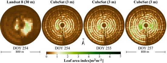
The spatial and temporal advantages afforded by daily CubeSat LAI imagery are further emphasized in a three-day sequence capturing the timing and progression of a harvesting event commenced on DOY 181 and completed on DOY 183 (Figure 8a). In this instance, Landsat LAI is only available on DOY 181, missing critical day-to-day dynamics in vegetation response. Similarly, Figure 8b demonstrates that the exact timing of the harvesting event on DOY 222 can only be inferred from a daily sequence of CubeSat images. While the single Landsat acquisition on DOY 222 captures this specific harvest event, the exact transition day would be impossible to determine based on imagery captured 8–16 days earlier. In addition, the spatial resolution of the Landsat LAI on DOY 222 is generally too coarse for delineating the harvested areas, or progress, with high accuracy. Figure 8c demonstrates the potential of detail-rich CubeSat data for capturing intrafield scale variability in LAI during a green-up phase (DOY 254–257) from an alfalfa field that exhibits significant fine-scale heterogeneity. The closely spaced (i.e., intervals of ~50 m) circular wheel tracks from the rotating center-pivot irrigation system add further complexity to the interpretation of vegetation response and plant development, but these features are effectively resolved by the CubeSat data. In comparison, Landsat LAI represent a mixed signal significantly confounded by bare soil contributions from the wheel tracks. In addition, the temporal insights afforded by 8–16-day Landsat data present a significant limitation during dynamic vegetative periods such as this.
4. Discussion
Constellations of CubeSats in low-earth orbits constitute an unprecedented opportunity to monitor the terrestrial surface with enhanced spatial detail more frequently than ever before. This study demonstrated the capacity of Planet’s constellation of CubeSats, equipped with basic optical imagers (i.e., RGB + NIR), to monitor vegetation dynamics at high spatial (~3 m) and temporal (~daily) resolution. While daily imaging was available during the majority of the six-month study period, original (i.e., not CESTEM corrected) NDVI time series over a multicut alfalfa field indicated significant day-to-day variations not directly attributable to vegetation dynamics or phenology. While atmospheric influences due to dust aerosols were significant, atmospheric correction did not reduce the high-frequency noise. Cross-sensor inconsistencies in radiometric quality, spectral responses, and orbital configuration are the likely contributors to the noise observed in this time-series record. Even though Planet’s constellation of CubeSats undergoes fairly rigorous radiometric calibrations, as outlined in Section 2.1, the residual noise, as demonstrated here, represents a notable limitation for high-fidelity land surface characterization. Additionally, the limited spectral information content contained in broad and partially overlapping bands is inconsistent with the narrower VNIR band configuration typical of conventional multispectral satellite systems such as Landsat and Sentinel-2 [33,61]. While Planet have recently implemented their own 6S-based atmospheric correction protocols, the product was not in wide distribution until October 2017, which is at the end of our study period. Importantly, Planet’s approach does not include adaptations to account for localized aerosol and adjacency effects, which are key factors in our (and many other) study environments. In any case, atmospheric correction of the CubeSat data is not a requirement for running CESTEM that can accept raw digital counts or TOA reflectances as demonstrated in this study.
CESTEM was designed to realize the full potential afforded by CubeSat resources and to allow high-quality, very high-resolution spatiotemporal insights. At its core, CESTEM serves as a radiometric normalization mechanism that has a demonstrated capacity to translate CubeSat observations into L8-consistent imagery, while retaining the radiometric quality of actual L8 observations [33]. In the current study, CESTEM effectively corrected the “raw” multitemporal CubeSat scene data into L8-consistent surface reflectance estimates using an 8–16-day Landsat record as reference data. With this normalized dataset, key phenometrics, such as the start, end, and length of five well-defined and rapidly evolving alfalfa growing seasons, could be accurately retrieved. What is pressingly evident is that Landsat data alone, even with the eight-day frequency available over parts of the study domain (Figure 1), are incapable of detecting the high-frequency vegetation dynamics characteristic of multicut alfalfa. More generally, the time-critical and spatially explicit information needs of precision agricultural management cannot typically be satisfied by conventional satellite resources alone. On the other hand, integrative multisource approaches based on CubeSat imaging hold the potential to overcome traditional spatiotemporal constraints.
Temporal smoothing filters can be highly useful for assessing vegetation phenology and calculating phenological transition dates from satellite time-series data [11]. However, the robustness of the phenology reconstruction can be very sensitive to the choice of smoothing algorithm and parameter calibration [62], and ultimately depends on the availability of a sufficient number of high quality observations during phenological transition events [63]. In this case, common smoothing filters for phenology reconstruction [64] would have limited utility given the real risk of mistaking some of the high-frequency NDVI dynamics (i.e., such as the dips in NDVI between alfalfa growing seasons) as signal contamination. The addition of five-day Sentinel-2 data would certainly increase the capacity of conventional satellite resources for high-resolution land surface characterization, particularly if used synergistically in the manner envisioned by the Harmonized Landsat Sentinel-2 initiative [27]. When combined together, a global median average revisit of 2.9 days can be achieved [25], which constitutes a major advance towards obtaining clear-sky imagery in a timely fashion. Still, the temporal frequency is in many cases suboptimal for monitoring rapid land cover and land use changes in near real time [30], which requires clear-sky image acquisitions immediately before and after the change event. Even disregarding the enhanced spatial resolution, with a daily imaging frequency, the potential of Planet’s constellation of CubeSats for monitoring day-to-day variations in vegetation dynamics and characteristics (after careful corrections for cross-sensor inconsistencies) is clearly demonstrated in this study. Importantly, CESTEM can also be adapted to only exploit satellite data acquired prior to the CubeSat prediction day (see Section 2.4.2), which would enable near real-time predictions needed in the context of precision agriculture.
Unavoidable impacts of cloud contamination on data availability may be partly mitigated by exploiting the expanding capability of the constellation to survey the same location more than once a day. In this manner, the frequency of observations will approximate the revisit capability of the two-satellite (i.e., Terra and Aqua) MODIS configuration, with a truly impressive factor of 80–160 increase in spatial resolution (i.e., 250/500 m to 3.125 m). In addition to disrupting the temporal continuity of the observational CubeSat record, atmospheric contamination may affect the robustness of CESTEM retrievals, as extended timespans between clear-sky L8 overpasses will reduce the number of representative reference samples. Over cloud-prone regions, an effective near real-time phenology reconstruction via CESTEM would probably require a longer multiyear record of searchable L8 scenes together with harmonized Sentinel-2 data continuously updated with new reference scenes as they become available. In this context, the weighting of reference samples drawn from multiple scenes serves to effectively smooth out noise in the time-series reference data. As such, CESTEM also functions as a superior phenological smoothing filter that draws from actual high-frequency (~daily) CubeSat observations without the uncertainties associated with traditional smoothing and gap-filling approximations [65].
In addition to enhanced temporal insights, the spatial detail afforded by the CubeSat data within the framework of CESTEM can be highly advantageous for agricultural management at the precision scale via actionable intrafield information on vegetation dynamics and disturbances. This potential was demonstrated on the basis of CubeSat-derived LAI using CESTEM as the mechanism to enhance Landsat-based LAI both spatially and temporally. The CubeSat resolution (~3 m) was able to resolve intrafield-scale spatial features largely absent in the Landsat retrievals, and daily sequences of CubeSat LAI highlighted rapid and detail-rich crop dynamics completely missed by the 8–16-day Landsat imagery. The adopted RF machine-learning approach was shown to reproduce the L8 reference LAI with high accuracy (i.e., relative MAD ranging from 3.5–6.4%) based on a relatively limited suite of spectral variables derivable from the CESTEM corrected VNIR data. This was despite the fact that a more spectrally enhanced dataset, including critical bands in the shortwave infrared domain, was needed for the Landsat-based LAI retrieval in order to reproduce observed multiday features with sufficient accuracy [41]. Robust CubeSat-based LAI retrievals were facilitated by strong associations between LAI and standard indices in the VNIR [66] in combination with a repeatable redefinition of RF prediction models based on scene-specific reference data. This approach exploits the powerful capacity of data-driven machine-learning techniques to reproduce spatially explicit features in “seen” observations (e.g., reference LAI) while reducing the impact of intrinsic portability and transferability issues [41,67]. As such, CESTEM-LAI takes advantage of high quality and spectrally enhanced sensor data (e.g., Landsat 8) for reference data generation, while reserving the more spectrally limited CubeSat data exclusively for spatiotemporal enhancement purposes.
The downscaling from 30 m to 3.125 m resolution can result in errors due to overfitting and poor generalization [68] and was constrained by employing simpler Cubist-based regression functions at the full resolution scale. In addition to improving computational speed, this approach ensures realistic distributions at the ~3 m scale without impacting magnitudes predicted by the more complex models at the 30 m resolution scale. Although the scene-specific machine-learning approach still represents a limitation when processing large amounts of satellite scenes, continued developments in cloud computing and improvements in data-driven techniques [14] could offer enhanced mapping efficiency and a pathway towards a larger-scale cloud implementation.
A future integration of Sentinel-2 data is likely to add an expanded capacity to other vegetation biophysical properties (i.e., chlorophyll content or carotenoids) which rely on the additional bands in the red-edge for well-constrained retrievals [46,69,70]. In this case, correlative associations between red-edge and combined green and NIR signals, via pigment and vegetation biomass interdependences [71,72], could ensure effective CubeSat-based parameter enhancement on a scene-specific basis [33]. Extendibility to hydrological process variables may also be envisioned, including evapotranspiration (ET), given its strong link to optical remote sensing data and derivable metrics of vegetation density [30]. However, the capacity of CESTEM to effectively resolve spatial variability in water use, considering the complex impacts of irrigation, water availability, and vegetation stress [73], remains to be investigated further. In that context, a comparative analysis against traditional data-fusion algorithms for enhancing observing capacity [16,21], necessitated by the long-standing trade-off between the spatial and temporal resolution of conventional satellites (e.g., Landsat versus MODIS), would be highly relevant. Since CubeSat constellations overcome these traditional spatiotemporal constraints (i.e., by providing Landsat-like data at MODIS frequency), the CESTEM approach offers a unique avenue towards spatiotemporal enhancement with potentially superior retrieval accuracy.
With the key focus being directed towards demonstrating the temporal and spatial advantages of emerging CubeSat resources for vegetation monitoring, a rigorous validation of CESTEM results against independent data was not performed. Elaborate evaluations of temporal LAI dynamics and retrieval robustness should involve continuous records of ground-based LAI automatically observed based on downward-looking digital photos [74,75], upward-looking digital cover photography [76], or indirectly via tower-mounted measurements of spectral vegetation index data [77]. Similarly, evaluations of CESTEM-derived NDVI phenology should include comparisons against continuous NDVI records observed via near-surface remote sensing with digital cameras mounted on towers [78,79,80], as embodied by the PhenoCam network [81]. The integration of ancillary high-frequency and very high spatial resolution (i.e., <5 m) taskable satellite (e.g., WorldView, GeoEye, VeNUS) or UAV resources may be envisioned as an independent mechanism towards a time and scale-relevant verification of spectral and vegetation biophysical features in the CESTEM-derived product suite.
5. Conclusions
Here, we demonstrated the potential of a constellation of CubeSats for providing daily insights into vegetation dynamics at ~3 m resolution. When using the original Planet data, cross-sensor inconsistencies due to variations in orbital configurations, spectral responses, and radiometric quality resulted in a relatively noisy six-month NDVI time series, making phenology reconstruction difficult and susceptible to large uncertainties. The CubeSat Enabled Spatio-Temporal Enhancement Method (CESTEM), based on a multisource (i.e., CubeSat, Landsat 8, MODIS) and multiscale (i.e., 3 m, 30 m, 500 m) machine-learning technique, facilitated radiometric normalization of CubeSat top of atmosphere (TOA) RGB + NIR data into Landsat-8-consistent surface reflectances. The CESTEM-corrected NDVI time series revealed clearly discernable and smoothly evolving growing cycles with a crop-growth period on the order of 30–40 days. These results highlighted the impressive capacity of near-daily CubeSat imaging for resolving high-frequency vegetation dynamics and determining the exact timing of key phenological transitions.
In addition to providing temporally consistent phenology information via NDVI, CESTEM demonstrated its potential for enhancing Landsat-based LAI both spatially and temporally, while maintaining consistency with Landsat-scale LAI. Daily sequences of CubeSat-based LAI highlighted the spatial resolution advantage and provided critical temporal insights into within-field variations in vegetation health and condition, the rate of vegetation green-up, and the timing and progress of harvesting events, features that were largely uncaptured by the 8–16-day Landsat imagery.
While CubeSat constellations are on path to reshape our earth-observing potential, the realization of their full potential will likely require synergistic exploration with conventional satellite systems. By serving as a multipurpose data-fusion scheme for radiometric normalization, time-series smoothing, and spatiotemporal enhancement of biophysical properties, CESTEM provides this needed framework and represents a novel paradigm with application potential across diverse aspects of earth observation. Optimization of mapping efficiency (e.g., via cloud computing) and rigorous evaluation of retrieval robustness and observing capacity over a wide range of ecosystems and environmental conditions constitute key objectives for future research.
Author Contributions
R.H. and M.F.M conceived the project. R.H. developed the algorithm and designed the framework, processed and analyzed the data, and prepared the figure material. R.H. wrote the paper with assistance from M.F.M.
Acknowledgments
We acknowledge Planet’s Ambassadors program and the associated access to their imagery archive, in addition to the outreach efforts and collaborative support of Planet’s Joseph Mascaro. We greatly appreciate the logistical, equipment, and scientific support offered to our team by Jack King, Alan King, and employees of the Tawdeehiya Farm in Al Kharj, Saudi Arabia, without whom this research would not have been possible. RH acknowledges research support by the South Dakota State University. MFM acknowledges the support provided by the King Abdullah University of Science and Technology, who funded aspects of this research.
Conflicts of Interest
The authors declare no conflict of interest. The founding sponsors had no role in the design of the study; in the collection, analyses, or interpretation of data; in the writing of the manuscript, and in the decision to publish the results.
References
- Wood, E.F.; Roundy, J.K.; Troy, T.J.; van Beek, L.P.H.; Bierkens, M.F.P.; Blyth, E.; de Roo, A.; Döll, P.; Ek, M.; Famiglietti, J.; et al. Hyperresolution global land surface modeling: Meeting a grand challenge for monitoring Earth’s terrestrial water. Water Resour. Res. 2011, 47. [Google Scholar] [CrossRef]
- Sheffield, J.; Wood, E.F.; Chaney, N.; Guan, K.; Sadri, S.; Yuan, X.; Olang, L.; Amani, A.; Ali, A.; Demuth, S.; et al. A drought monitoring and forecasting system for Sub-Sahara African water resources and food security. Bull. Am. Meteorol. Soc. 2014, 95, 861–882. [Google Scholar] [CrossRef]
- Roy, D.P.; Wulder, M.A.; Loveland, T.R.; Woodcock, C.E.; Allen, R.G.; Anderson, M.C.; Helder, D.; Irons, J.R.; Johnson, D.M.; Kennedy, R.; et al. Landsat-8: Science and product vision for terrestrial global change research. Remote Sens. Environ. 2014, 145, 154–172. [Google Scholar] [CrossRef]
- Schmidhuber, J.; Tubiello, F.N. Global food security under climate change. Proc. Natl. Acad. Sci. USA 2007, 104, 19703–19708. [Google Scholar] [CrossRef] [PubMed] [Green Version]
- Burke, M.; Lobell, D.B. Satellite-based assessment of yield variation and its determinants in smallholder African systems. Proc. Natl. Acad. Sci. USA 2017, 114, 2189–2194. [Google Scholar] [CrossRef] [PubMed] [Green Version]
- Atzberger, C. Advances in remote sensing of agriculture: Context description, existing operational monitoring systems and major information needs. Remote Sens. 2013, 5, 949–981. [Google Scholar] [CrossRef]
- Becker-Reshef, I.; Justice, C.; Sullivan, M.; Vermote, E.; Tucker, C.; Anyamba, A.; Small, J.; Pak, E.; Masuoka, E.; Schmaltz, J.; et al. Monitoring Global Croplands with Coarse Resolution Earth Observations: The Global Agriculture Monitoring (GLAM) Project. Remote Sens. 2010, 2, 1589–1609. [Google Scholar] [CrossRef] [Green Version]
- Gebbers, R.; Adamchuk, V.I. Precision Agriculture and Food Security. Science 2010, 327, 828–831. [Google Scholar] [CrossRef] [PubMed]
- Moran, M.S.; Inoue, Y.; Barnes, E.M. Opportunities and limitations for image-based remote sensing in precisions crop management. Remote Sens. Environ. 1997, 61, 319–346. [Google Scholar] [CrossRef]
- Reed, B.C.; Brown, J.F.; VanderZee, D.; Loveland, T.R.; Merchant, J.W.; Ohlen, D.O. Measuring phenological variability from satellite imagery. J. Veg. Sci. 1994, 5, 703–714. [Google Scholar] [CrossRef]
- Zhang, X.; Friedl, M.A.; Schaaf, C.B.; Strahler, A.H.; Hodges, J.C.F.; Gao, F.; Reed, B.C.; Huete, A. Monitoring vegetation phenology using MODIS. Remote Sens. Environ. 2003, 84, 471–475. [Google Scholar] [CrossRef]
- Houborg, R.; Fisher, J.B.; Skidmore, A.K. Advances in remote sensing of vegetation function and traits. Int. J. Appl. Earth Obs. Geoinf. 2015, 43, 1–6. [Google Scholar] [CrossRef] [Green Version]
- Belward, A.S.; Skøien, J.O. Who launched what, when and why; trends in global land-cover observation capacity from civilian earth observation satellites. ISPRS J. Photogramm. Remote Sens. 2015, 103, 115–128. [Google Scholar] [CrossRef]
- McCabe, M.F.; Rodell, M.; Alsdorf, D.E.; Miralles, D.G.; Uijlenhoet, R.; Wagner, W.; Lucieer, A.; Houborg, R.; Verhoest, N.E.C.; Franz, T.E.; et al. The future of Earth observation in hydrology. Hydrol. Earth Syst. Sci. 2017, 21, 3879–3914. [Google Scholar] [CrossRef] [Green Version]
- Roy, D.P.; Ju, J.; Lewis, P.; Schaaf, C.; Gao, F.; Hansen, M.; Lindquist, E. Multi-temporal MODIS–Landsat data fusion for relative radiometric normalization, gap filling, and prediction of Landsat data. Remote Sens. Environ. 2008, 112, 3112–3130. [Google Scholar] [CrossRef]
- Gao, F.; Masek, J.; Schwaller, M.; Hall, F. On the blending of the Landsat and MODIS surface reflectance: Predicting daily Landsat surface reflectance. IEEE Trans. Geosci. Remote Sens. 2006, 44, 2207–2218. [Google Scholar]
- Emelyanova, I.V.; McVicar, T.R.; Van Niel, T.G.; Li, L.T.; van Dijk, A.I.J.M. Assessing the accuracy of blending Landsat-MODIS surface reflectances in two landscapes with contrasting spatial and temporal dynamics: A framework for algorithm selection. Remote Sens. Environ. 2013, 133, 193–209. [Google Scholar] [CrossRef]
- Hilker, T.; Wulder, M.A.; Coops, N.C.; Seitz, N.; White, J.C.; Gao, F.; Masek, J.G.; Stenhouse, G. Generation of dense time series synthetic Landsat data through data blending with MODIS using a spatial and temporal adaptive reflectance fusion model. Remote Sens. Environ. 2009, 113, 1988–1999. [Google Scholar] [CrossRef]
- Houborg, R.; McCabe, M.F.; Gao, F. A Spatio-Temporal Enhancement Method for medium resolution LAI (STEM-LAI). Int. J. Appl. Earth Obs. Geoinf. 2016, 47, 15–29. [Google Scholar] [CrossRef] [Green Version]
- Weng, Q.; Fu, P.; Gao, F. Generating daily land surface temperature at Landsat resolution by fusing Landsat and MODIS data. Remote Sens. Environ. 2014, 145, 55–67. [Google Scholar] [CrossRef]
- Cammalleri, C.; Anderson, M.C.; Gao, F.; Hain, C.R.; Kustas, W.P. Mapping daily evapotranspiration at field scales over rainfed and irrigated agricultural areas using remote sensing data fusion. Agric. For. Meteorol. 2014, 186, 1–11. [Google Scholar] [CrossRef]
- Semmens, K.A.; Anderson, M.C.; Kustas, W.P.; Gao, F.; Alfieri, J.G.; McKee, L.; Prueger, J.H.; Hain, C.R.; Cammalleri, C.; Yang, Y.; et al. Monitoring daily evapotranspiration over two California vineyards using Landsat 8 in a multi-sensor data fusion approach. Remote Sens. Environ. 2016, 185, 155–170. [Google Scholar] [CrossRef] [Green Version]
- Houborg, R.; McCabe, M.F. Impacts of dust aerosol and adjacency effects on the accuracy of Landsat 8 and RapidEye surface reflectances. Remote Sens. Environ. 2017, 194, 127–145. [Google Scholar] [CrossRef]
- Drusch, M.; Del Bello, U.; Carlier, S.; Colin, O.; Fernandez, V.; Gascon, F.; Hoersch, B.; Isola, C.; Laberinti, P.; Martimort, P.; et al. Sentinel-2: ESA’s Optical High-Resolution Mission for GMES Operational Services. Remote Sens. Environ. 2012, 120, 25–36. [Google Scholar] [CrossRef]
- Li, J.; Roy, D.P. A global analysis of Sentinel-2A, Sentinel-2B and Landsat-8 data revisit intervals and implications for terrestrial monitoring. Remote Sens. 2017, 9, 902. [Google Scholar] [CrossRef]
- Yan, L.; Roy, D.P.; Zhang, H.; Li, J.; Huang, H. An Automated Approach for Sub-Pixel Registration of Landsat-8 Operational Land Imager (OLI) and Sentinel-2 Multi Spectral Instrument (MSI) Imagery. Remote Sens. 2016, 8, 520. [Google Scholar] [CrossRef]
- Harmonized Landsat Sentinel-2. Available online: https://hls.gsfc.nasa.gov/ (accessed on 14 March 2018).
- Puig-Suari, J.; Turner, C.; Ahlgren, W. Development of the standard CubeSat deployer and a CubeSat class PicoSatellite. In Proceedings of the 2001 IEEE Aerospace Conference Proceedings (Cat. No.01TH8542), Big Sky, MT, USA, 10–17 March 2001; Volume 1, pp. 1/347–1/353. [Google Scholar]
- Selva, D.; Krejci, D. A survey and assessment of the capabilities of Cubesats for Earth observation. Acta Astronaut. 2012, 74, 50–68. [Google Scholar] [CrossRef]
- McCabe, M.F.; Aragon, B.; Houborg, R.; Mascaro, J. CubeSats in Hydrology: Ultrahigh-Resolution Insights Into Vegetation Dynamics and Terrestrial Evaporation. Water Resour. Res. 2017, 53, 10017–10024. [Google Scholar] [CrossRef]
- Planet Team. Planet Application Program Interface. In Space for Life on Earth; Planet Team: San Francisco, CA, USA, 2017; Available online: https://api.planet.com (accessed on 6 June 2018).
- Houborg, R.; McCabe, M.F. High-Resolution NDVI from Planet’s Constellation of Earth Observing Nano-Satellites: A New Data Source for Precision Agriculture. Remote Sens. 2016, 8, 768. [Google Scholar] [CrossRef]
- Houborg, R.; McCabe, M.F. A Cubesat enabled Spatio-Temporal Enhancement Method (CESTEM) utilizing Planet, Landsat and MODIS data. Remote Sens. Environ. 2018, 209, 211–226. [Google Scholar] [CrossRef]
- Madugundu, R.; Al-Gaadi, K.A.; Tola, E.K.; Hassaballa, A.A.; Patil, V.C. Performance of the METRIC model in estimating evapotranspiration fluxes over an irrigated field in Saudi Arabia using Landsat-8 images. Hydrol. Earth Syst. Sci. 2017, 21, 6135–6151. [Google Scholar] [CrossRef] [Green Version]
- Rosas, J.; Houborg, R.; McCabe, M.F. Sensitivity of Landsat 8 surface temperature estimates to atmospheric profile data: A study using MODTRAN in dryland irrigated systems. Remote Sens. 2017, 9, 988. [Google Scholar] [CrossRef]
- Planet Imagery Product Specification. Available online: https://www.planet.com/products/satellite-imagery/files/Planet_Combined_Imagery_Product_Specs_December2017.pdf (accessed on 6 June 2018).
- Nicholas, W.; Greenberg, J.; Jumpasut, A.; Collison, A.; Weichelt, H. Absolute Radiometric Calibration of Planet Dove Satellites, Flocks 2p & 2e; Planet Labs: San Francisco, CA, USA, 2017; pp. 1–13. [Google Scholar]
- USGS Landsat Collections. Available online: https://landsat.usgs.gov/landsat-collections (accessed on 6 June 2018).
- Kotchenova, S.Y.; Vermote, E.F.; Matarrese, R.; Klemm, F.J. Validation of a vector version of the 6S radiative transfer code for atmospheric correction of satellite data. Part I: Path radiance. Appl. Opt. 2006, 45, 6762–74. [Google Scholar] [CrossRef] [PubMed]
- Vermote, E.F.; Tanre, D.; Deuze, J.L.; Herman, M.; Morcrette, J.-J. Second simulation of the satellite signal in the solar spectrum, 6s: An overview. IEEE Trans. Geosci. Remote Sens. 1997, 35, 675–686. [Google Scholar] [CrossRef]
- Houborg, R.; McCabe, M.F. A hybrid training approach for leaf area index estimation via Cubist and random forests machine-learning. ISPRS J. Photogramm. Remote Sens. 2018, 135, 173–188. [Google Scholar] [CrossRef]
- RuleQuest. Available online: http://www.rulequest.com (accessed on 14 March 2018).
- Quinlan, J.R. Learning with continuous classes. In Proceedings of the Fifth International Conference Artificial Intelligence; Springer: Singapore, Singapore, 1992; Volume 92, pp. 343–348. [Google Scholar]
- Quinlan, J.R. Combining instance-based and model-based learning. In Proceedings of the Tenth International Conference on Machine Learning, Amherst, MA, USA, 27–29 June 1993; pp. 236–343. [Google Scholar]
- Quinlan, J.R. Improved use of continuous attributes in C4. 5. J. Artif. Intell. Res. 1996, 4, 77–90. [Google Scholar]
- Houborg, R.; McCabe, M.F. Adapting a regularized canopy reflectance model (REGFLEC) for the retrieval challenges of dryland agricultural systems. Remote Sens. Environ. 2016, 186, 105–120. [Google Scholar] [CrossRef]
- Schaaf, C. MCD43A4 MODIS/Terra+Aqua BRDF/Albedo Nadir BRDF Adjusted RefDaily L3 Global - 500m V006. NASA EOSDIS Land Processes DAAC. Available online: https://doi.org/10.5067/modis/mcd43a4.006 (accessed on 14 March 2018).
- Schaaf, C.B.; Gao, F.; Strahler, A.H.; Lucht, W.; Li, X.; Tsang, T.; Strugnell, N.C.; Zhang, X.; Jin, Y.; Muller, J.-P.; et al. First operational BRDF, albedo nadir reflectance products from MODIS. Remote Sens. Environ. 2002, 83, 135–148. [Google Scholar] [CrossRef] [Green Version]
- MODIS Land Team. Validation Status for: BRDF/Albedo (MCD43). Available online: https://landval.gsfc.nasa.gov/ProductStatus.php?ProductID=MOD43 (accessed on 14 March 2018).
- Python Fmask. Available online: http://pythonfmask.org/en/latest/ (accessed on 14 March 2018).
- Zhu, Z.; Wang, S.; Woodcock, C.E. Improvement and expansion of the Fmask algorithm: Cloud, cloud shadow, and snow detection for Landsats 4–7, 8, and Sentinel 2 images. Remote Sens. Environ. 2015, 159, 269–277. [Google Scholar] [CrossRef]
- Rouse, J.W.; Hass, R.H.; Shell, J.A.; Deering, D. Monitoring vegetation systems in the Great Plains with ERTS-1. In Third Earth Resources Technologhy Satellite Symposium; NASA: Washington, DC, USA, 1973; Volume 351, pp. 309–317. [Google Scholar]
- Huete, A.R. A soil-adjusted vegetation index (SAVI). Remote Sens. Environ. 1988, 25, 295–309. [Google Scholar] [CrossRef]
- Gitelson, A.A.; Merzlyak, M.N. Remote sensing of chlorophyll concentration in higher plant leaves. Adv. Space Res. 1998, 22, 689–692. [Google Scholar] [CrossRef]
- Haboudane, D.; Miller, J.R.; Pattey, E.; Zarco-Tejada, P.J.; Strachan, I.B. Hyperspectral vegetation indices and novel algorithms for predicting green LAI of crop canopies: Modeling and validation in the context of precision agriculture. Remote Sens. Environ. 2004, 90, 337–352. [Google Scholar] [CrossRef]
- Sripada, R.P.; Heiniger, R.W.; White, J.G.; Meijer, A.D. Aerial color infrared photography for determining early in-season nitrogen requirements in corn. Agron. J. 2006, 98, 968–977. [Google Scholar] [CrossRef]
- Breiman, L. Random Forests. Mach. Learn. 2001, 45, 5–32. [Google Scholar] [CrossRef] [Green Version]
- Gupta, V.; Fard, A.; Li, W.; Saltz, M. Package randomForest.ddr. Available online: https://cran.r-project.org/web/packages/randomForest.ddR/randomForest.ddR.pdf (accessed on 14 March 2018).
- Liaw, A.; Wiener, M. Classification and Regression by randomForest. R News 2002, 2, 18–22. [Google Scholar]
- Li, S.; Dragicevic, S.; Castro, F.A.; Sester, M.; Winter, S.; Coltekin, A.; Pettit, C.; Jiang, B.; Haworth, J.; Stein, A.; et al. Geospatial big data handling theory and methods: A review and research challenges. ISPRS J. Photogramm. Remote Sens. 2016, 115, 119–133. [Google Scholar] [CrossRef] [Green Version]
- Goetz, A.F.H.; Vane, G.; Solomon, J.E.; Rock, B.N. Imaging Spectrometry for Earth Remote Sensing. Science 1985, 228, 1147–1153. [Google Scholar] [CrossRef] [PubMed]
- Cai, Z.; Jönsson, P.; Jin, H.; Eklundh, L. Performance of smoothing methods for reconstructing NDVI time-series and estimating vegetation phenology from MODIS data. Remote Sens. 2017, 9, 1271. [Google Scholar] [CrossRef]
- Zhang, X.; Friedl, M.A.; Schaaf, C.B. Global vegetation phenology from Moderate Resolution Imaging Spectroradiometer (MODIS): Evaluation of global patterns and comparison with in situ measurements. J. Geophys. Res. Biogeosci. 2006, 111, 1–14. [Google Scholar] [CrossRef]
- Eklundh, L.; Jönsson, P. TIMESAT: A Software Package for Time-Series Processing and Assessment of Vegetation Dynamics; Springer: Cham, Switzerland, 2015; pp. 141–158. [Google Scholar]
- Kandasamy, S.; Baret, F.; Verger, A.; Neveux, P.; Weiss, M. A comparison of methods for smoothing and gap filling time series of remote sensing observations–application to MODIS LAI products. Biogeosciences 2013, 10, 4055–4071. [Google Scholar]
- Turner, D.P.; Cohen, W.B.; Kennedy, R.E.; Fassnacht, K.S.; Briggs, J.M. Relationships between leaf area index and Landsat TM spectral vegetation indices across three temperate zone sites. Remote Sens. Environ. 1999, 70, 52–68. [Google Scholar] [CrossRef]
- Vuolo, F.; Neugebauer, N.; Bolognesi, S.F.; Atzberger, C.; D’Urso, G. Estimation of leaf area index using DEIMOS-1 data: Application and transferability of a semi-empirical relationship between two agricultural areas. Remote Sens. 2013, 5, 1274–1291. [Google Scholar] [CrossRef]
- Srivastava, P.K.; Han, D.; Ramirez, M.R.; Islam, T. Machine Learning Techniques for Downscaling SMOS Satellite Soil Moisture Using MODIS Land Surface Temperature for Hydrological Application. Water Resour. Manag. 2013, 27, 3127–3144. [Google Scholar] [CrossRef]
- Clevers, J.G.P.W.; Gitelson, A.A. Remote estimation of crop and grass chlorophyll and nitrogen content using red-edge bands on sentinel-2 and-3. Int. J. Appl. Earth Obs. Geoinf. 2013, 23, 344–351. [Google Scholar] [CrossRef]
- Frampton, W.J.; Dash, J.; Watmough, G.; Milton, E.J. Evaluating the capabilities of Sentinel-2 for quantitative estimation of biophysical variables in vegetation. ISPRS J. Photogramm. Remote Sens. 2013, 82, 83–92. [Google Scholar] [CrossRef]
- Gitelson, A.A. Remote estimation of leaf area index and green leaf biomass in maize canopies. Geophys. Res. Lett. 2003, 30, 4–7. [Google Scholar] [CrossRef]
- Nguy-Robertson, A.L.; Gitelson, A.A. Algorithms for estimating green leaf area index in C3 and C4 crops for MODIS, Landsat TM/ETM+, MERIS, Sentinel MSI/OLCI, and Venµs sensors. Remote Sens. Lett. 2015, 6, 360–369. [Google Scholar] [CrossRef]
- Anderson, M.C.; Norman, J.M.; Kustas, W.P.; Houborg, R.; Starks, P.J.; Agam, N. A thermal-based remote sensing technique for routine mapping of land-surface carbon, water and energy fluxes from field to regional scales. Remote Sens. Environ. 2008, 112, 4227–4241. [Google Scholar] [CrossRef]
- Fang, H.; Ye, Y.; Liu, W.; Wei, S.; Ma, L. Continuous estimation of canopy leaf area index (LAI) and clumping index over broadleaf crop fields: An investigation of the PASTIS-57 instrument and smartphone applications. Agric. For. Meteorol. 2018, 253–254, 48–61. [Google Scholar] [CrossRef]
- Baret, F.; de Solan, B.; Lopez-Lozano, R.; Ma, K.; Weiss, M. GAI estimates of row crops from downward looking digital photos taken perpendicular to rows at 57.5° zenith angle: Theoretical considerations based on 3D architecture models and application to wheat crops. Agric. For. Meteorol. 2010, 150, 1393–1401. [Google Scholar] [CrossRef]
- Ryu, Y.; Verfaillie, J.; Macfarlane, C.; Kobayashi, H.; Sonnentag, O.; Vargas, R.; Ma, S.; Baldocchi, D.D. Continuous observation of tree leaf area index at ecosystem scale using upward-pointing digital cameras. Remote Sens. Environ. 2012, 126, 116–125. [Google Scholar] [CrossRef]
- Wilson, T.B.; Meyers, T.P. Determining vegetation indices from solar and photosynthetically active radiation fluxes. Agric. For. Meteorol. 2007, 144, 160–179. [Google Scholar] [CrossRef]
- Richardson, A.; Braswell, B. Near-surface remote sensing of spatial and temporal variation in canopy phenology. Ecol. Appl. 2009, 19, 1417–1428. [Google Scholar] [CrossRef] [PubMed]
- Filippa, G.; Cremonese, E.; Migliavacca, M.; Galvagno, M.; Sonnentag, O.; Humphreys, E.; Hufkens, K.; Ryu, Y.; Verfaillie, J.; Morra di Cella, U.; et al. NDVI derived from near-infrared-enabled digital cameras: Applicability across different plant functional types. Agric. For. Meteorol. 2018, 249, 275–285. [Google Scholar] [CrossRef]
- Liu, Y.; Hill, M.J.; Zhang, X.; Wang, Z.; Richardson, A.D.; Hufkens, K.; Filippa, G.; Baldocchi, D.D.; Ma, S.; Verfaillie, J.; et al. Using data from Landsat, MODIS, VIIRS and PhenoCams to monitor the phenology of California oak/grass savanna and open grassland across spatial scales. Agric. For. Meteorol. 2017, 237–238, 311–325. [Google Scholar] [CrossRef]
- Phenocam. Available online: https://phenocam.sr.unh.edu/webcam/ (accessed on 14 March 2018).
Figure 1.
Domain and geographic location of the studied agricultural farming area. The image is a false color representation of ~3 m resolution CubeSat RGB + NIR imagery. Zones with an 8-day, 8–16-day, and 16-day Landsat revisit frequency are overplotted. The alfalfa study unit (180 × 180 m2) used for extracting time series information is also indicated.

Figure 2.
Overview of CESTEM processing steps for producing Landsat 8 (L8) consistent multispectral and LAI information at the spatial and temporal resolution of the PlanetScope (PS) CubeSat data. Box colors indicate the spatial data resolution (i.e., native or resampled) at each processing step. See Section 2.4 for a detailed description of the methodology and parameter definitions.

Figure 3.
(a) Sensor view angle and local overpass time for clear-sky CubeSat imagery acquired over a six-month period. The insert depicts the frequency distribution of the number of days between consecutive CubeSat acquisitions. (b) Time series of aerosol optical thickness at 550 nm (AOT) derived from MODIS deep blue algorithm retrievals (Section 2.2) and used for the atmospheric correction of Landsat and PlanetScope data.

Figure 4.
(a) Six-month time series of Landsat 8 (L8) and PlanetScope (PS) NDVI calculated from atmospherically corrected (6SV) and top of atmosphere (TOA) reflectances. The data represent an alfalfa plot unit measuring 180 × 180 m2 (Figure 1). (b) CESTEM-corrected time series of PS NDVI based on 16-day L8 reference data (i.e., dependent scenes). The hollow L8 squares (i.e., independent scenes) were not used in CESTEM. The downscaled MODIS data (MOD) were used after bias correction (MOD_L8) (Section 2.4.2) to determine the relative change in surface reflectance over given CubeSat–Landsat acquisition timespans. (c) As in (b), except that reference data were drawn from the full eight-day L8 record.

Figure 5.
(a) Maps of 30 m resolution LAI based on Landsat 8 (L8) (top) and CubeSat (bottom) data acquired on day of year (DOY) 293. CubeSat LAI was derived via random forest machine-learning using L8 LAI as reference (see Section 2.4.4). (b) Density scatter plot intercomparing CubeSat and L8-based LAI on DOY 293. Statistical performance metrics are indicated on the plot and include the coefficient of determination (R2), the mean absolute difference (MAD), and the relative mean bias difference (rMBD). (c) Box-and-whisker plot that displays the minimum, lower quartile, median, upper quartile, and maximum of the MADs between CubeSat and L8 as a function of LAI. See Table 1 for the definitions of MAD and rMBD.

Figure 6.
CESTEM-based time series of PlanetScope (PS) LAI for the alfalfa study-unit (Figure 1) using eight-day Landsat 8 (L8) reference data (i.e., dependent scenes). Retrievals from the four L8 scenes not included in CESTEM (i.e., independent scenes) are also shown. The dashed line depicts the initial LAI series used to quantify the change in LAI over given CubeSat–Landsat acquisition timespans as part of the reference sampling scheme (Section 2.4.4). The shaded area indicates the vegetative period used for illustrative purposes in Figure 7.

Figure 7.
Daily sequence of 3 m resolution PlanetScope (PS) LAI bounded by 30 m resolution Landsat 8 (L8) retrievals on DOY 206 and 213. The imagery captures a vegetative phase in the alfalfa field as indicated by the shaded area in Figure 6.
Figure 7.
Daily sequence of 3 m resolution PlanetScope (PS) LAI bounded by 30 m resolution Landsat 8 (L8) retrievals on DOY 206 and 213. The imagery captures a vegetative phase in the alfalfa field as indicated by the shaded area in Figure 6.

Figure 8.
Events of rapid (i.e., from day to day) change in LAI over selected pivots across the study domain. (a) Timing of a harvesting event captured by daily PlanetScope (PS) LAI (DOY 180–183) whereas L8 LAI is only available on DOY 181. (b) Timing of intrafield transitions from high to low LAI captured by daily PS LAI (DOY 220–222) whereas L8 LAI is only available on DOY 222. (c) Rapid green-up development tracked by PS LAI (DOY 254–257) whereas L8 LAI is only available on DOY 254.


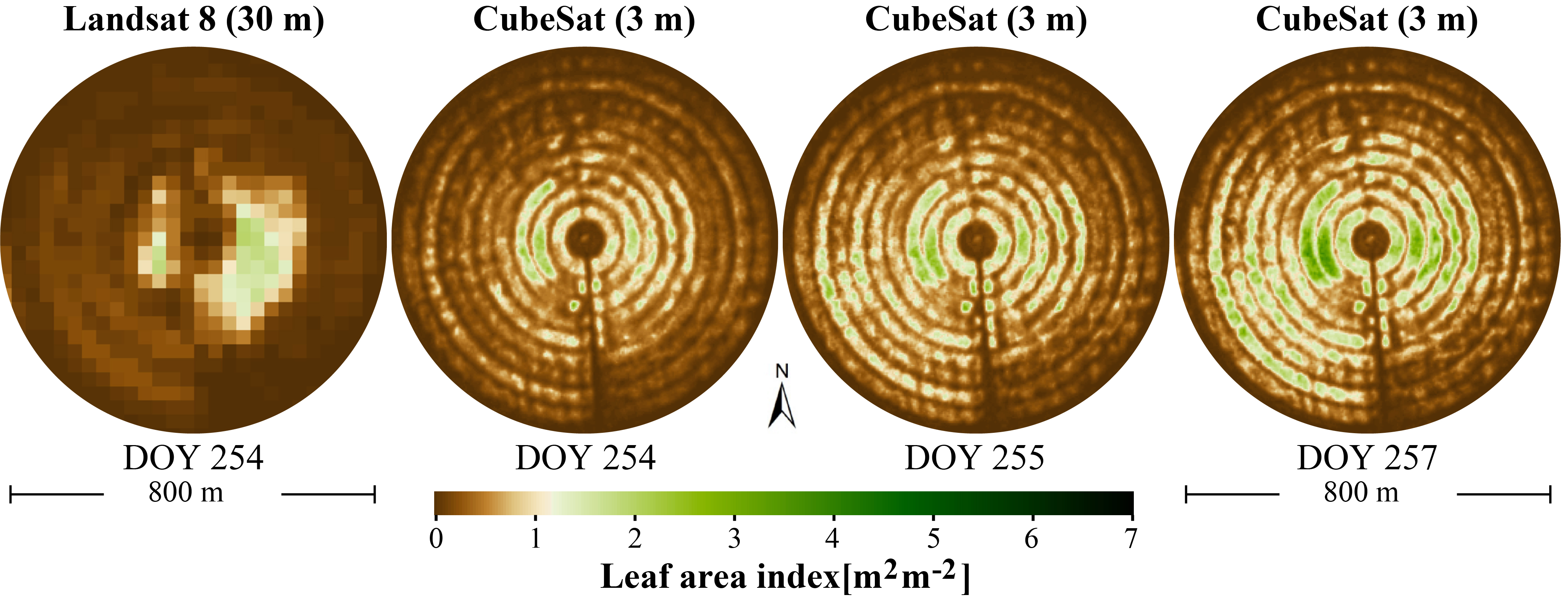
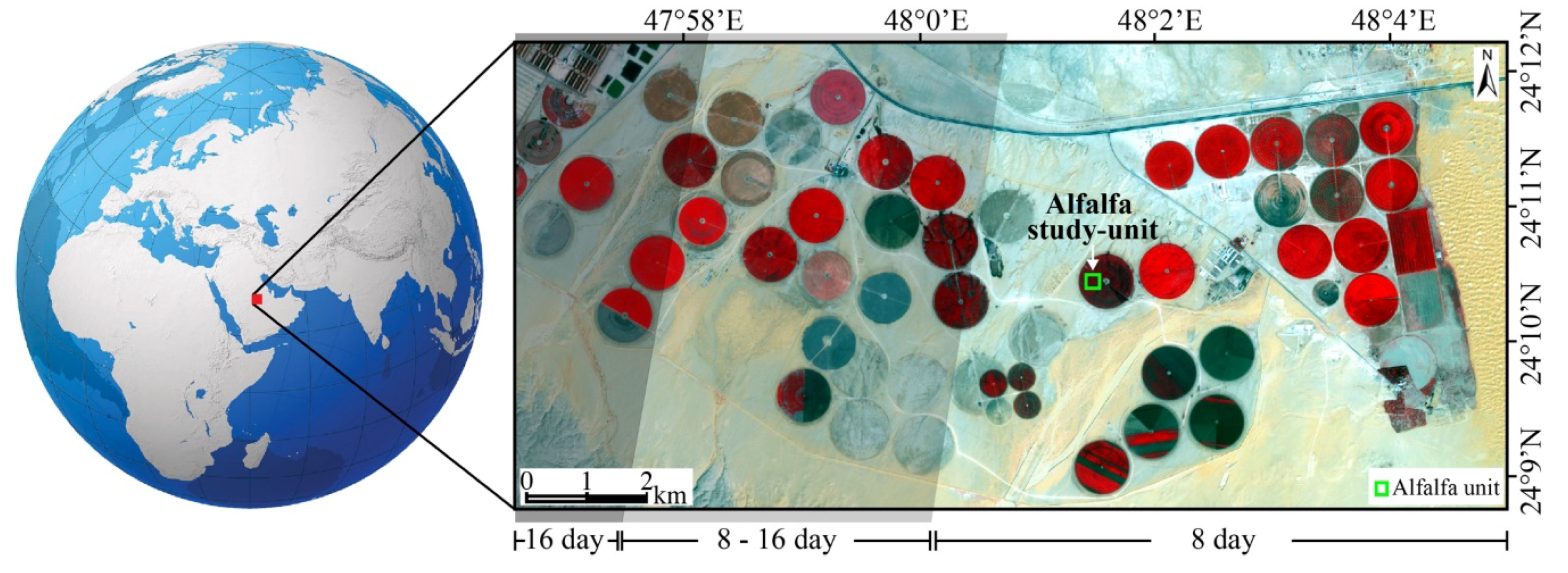
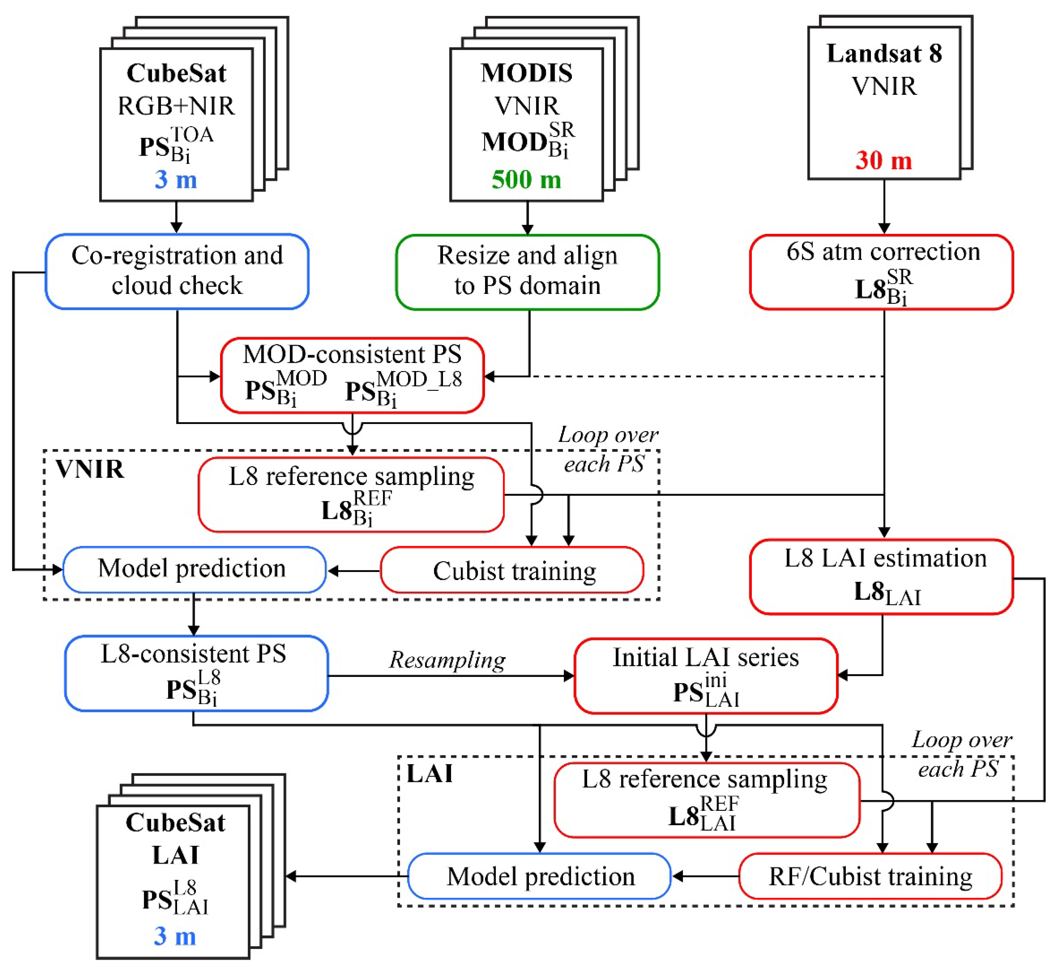
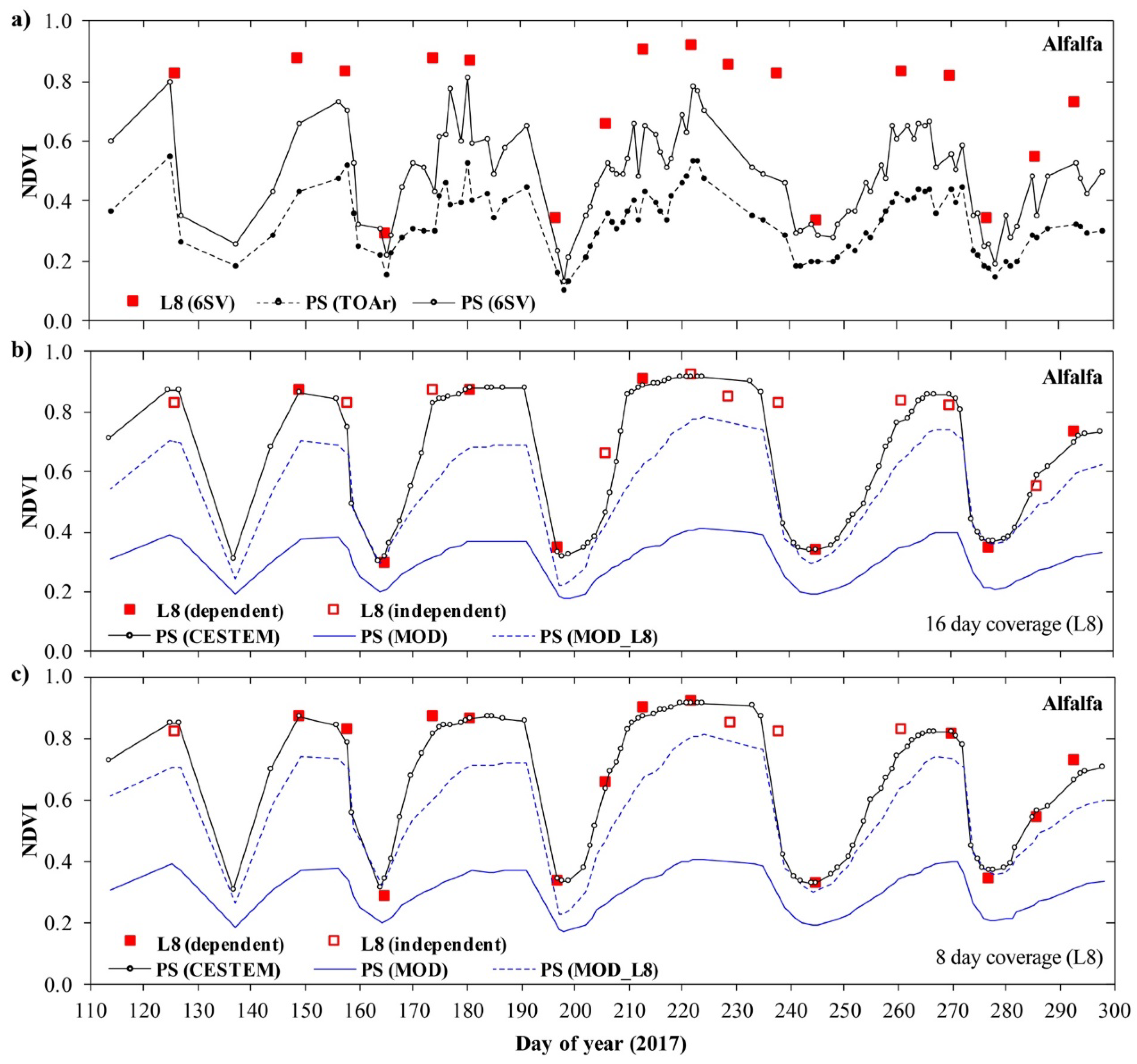
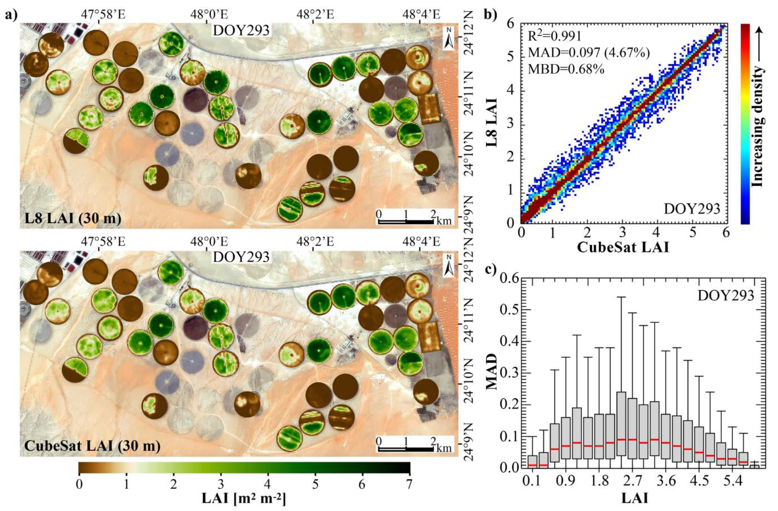
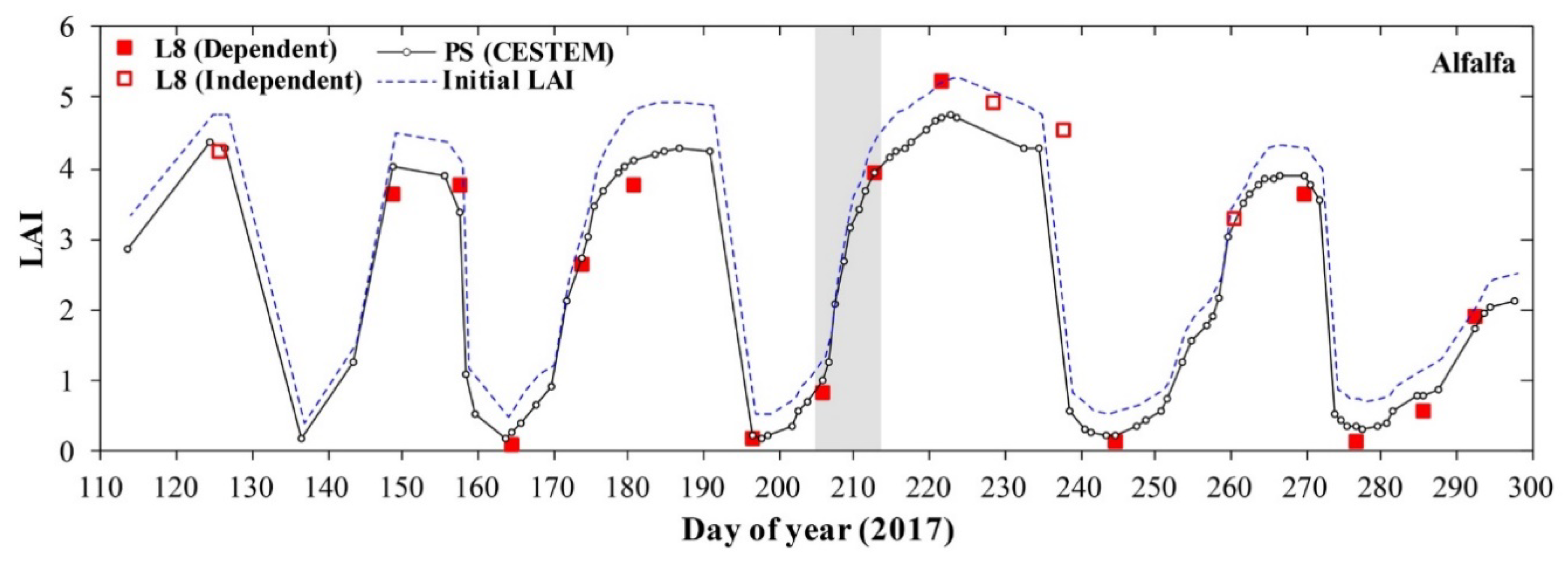
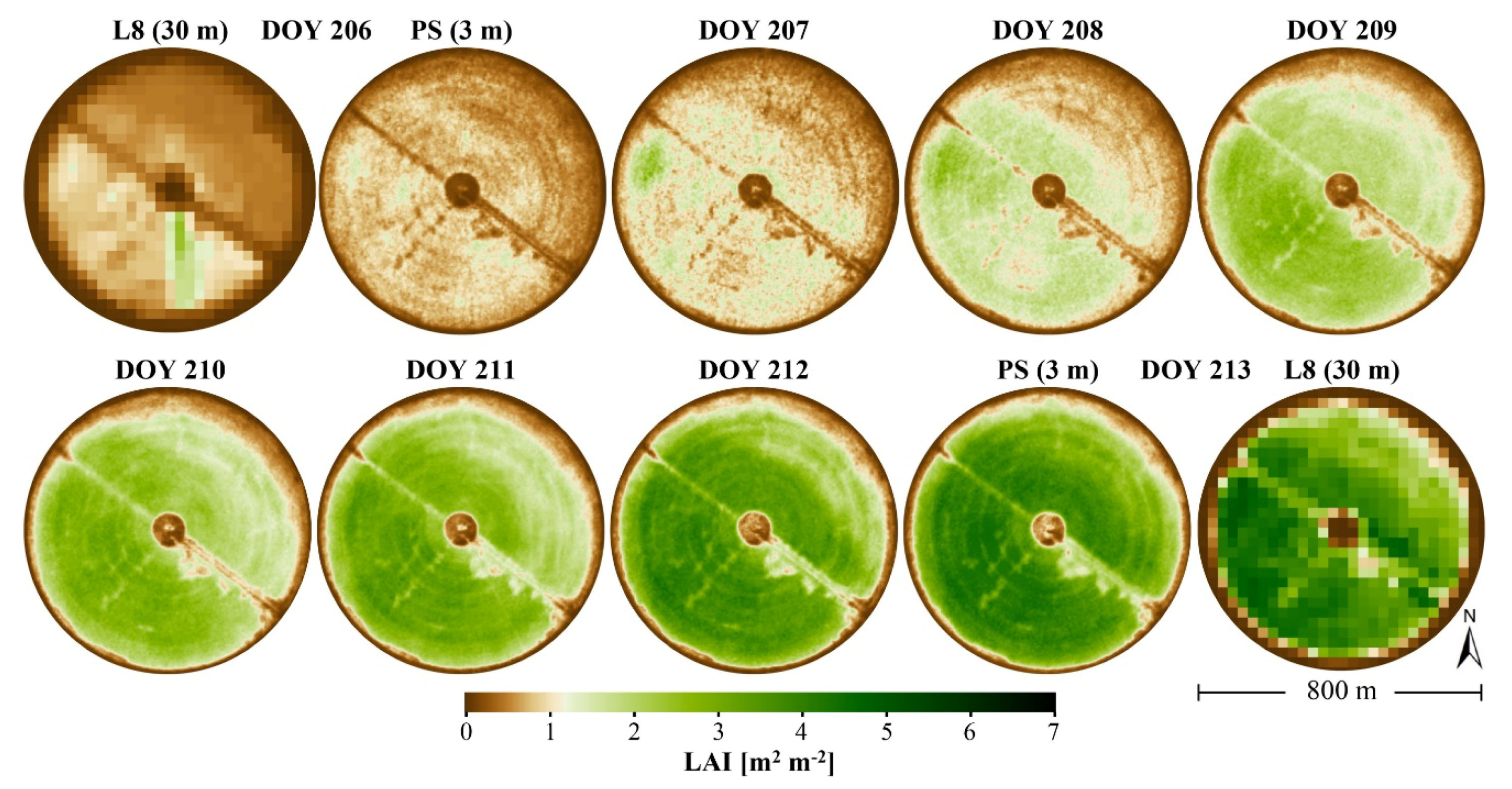
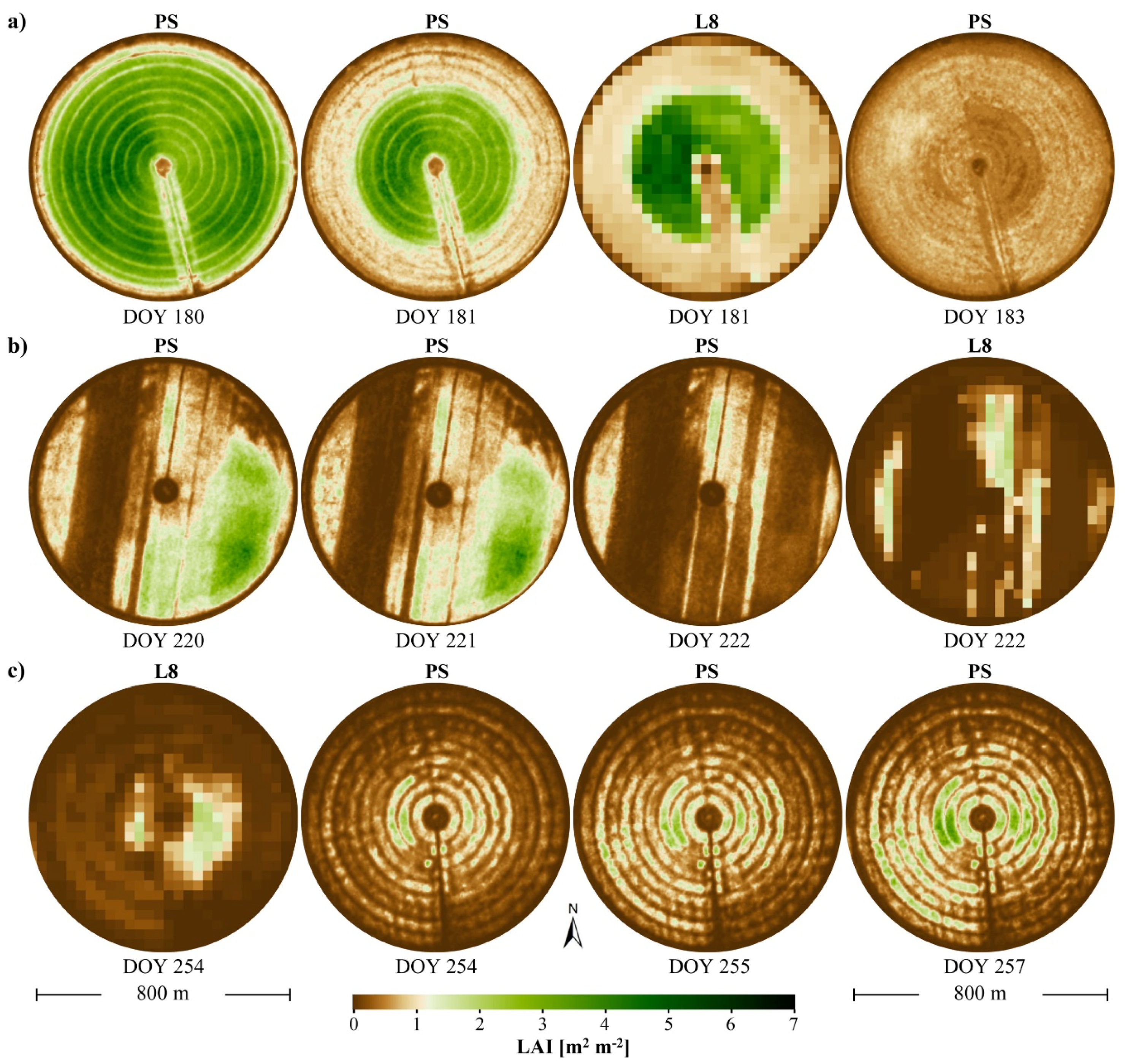
Table 1.
Statistical metrics of the agreement between Landsat 8 and CubeSat-based LAI during day-coincident acquisitions. Evaluations were performed at the 30 m scale (excluding desert pixels) and include the coefficient of determination (R2), the mean absolute difference (MAD), the relative MAD (rMAD), and the relative mean bias difference (rMBD). , , .
| DOY | 149 | 158 | 165 | 174 | 181 | 197 | 206 | 213 | 222 | 245 | 270 | 277 | 286 | 293 |
|---|---|---|---|---|---|---|---|---|---|---|---|---|---|---|
| R2 | 0.989 | 0.986 | 0.993 | 0.995 | 0.992 | 0.989 | 0.995 | 0.989 | 0.984 | 0.996 | 0.993 | 0.994 | 0.994 | 0.991 |
| MAD | 0.118 | 0.098 | 0.057 | 0.086 | 0.066 | 0.082 | 0.039 | 0.081 | 0.092 | 0.064 | 0.074 | 0.071 | 0.072 | 0.097 |
| rMAD [%] | 4.68 | 4.69 | 3.48 | 3.86 | 4.35 | 5.81 | 4.88 | 6.30 | 6.40 | 4.07 | 3.92 | 4.39 | 3.90 | 4.67 |
| rMBD [%] | 0.46 | −0.93 | 0.13 | 0.22 | 0.53 | 1.02 | 0.82 | 1.57 | −1.20 | 0.52 | 0.12 | 0.57 | 0.31 | 0.68 |
© 2018 by the authors. Licensee MDPI, Basel, Switzerland. This article is an open access article distributed under the terms and conditions of the Creative Commons Attribution (CC BY) license (http://creativecommons.org/licenses/by/4.0/).
Share and Cite
MDPI and ACS Style
Houborg, R.; McCabe, M.F. Daily Retrieval of NDVI and LAI at 3 m Resolution via the Fusion of CubeSat, Landsat, and MODIS Data. Remote Sens. 2018, 10, 890. https://doi.org/10.3390/rs10060890
AMA Style
Houborg R, McCabe MF. Daily Retrieval of NDVI and LAI at 3 m Resolution via the Fusion of CubeSat, Landsat, and MODIS Data. Remote Sensing. 2018; 10(6):890. https://doi.org/10.3390/rs10060890
Chicago/Turabian StyleHouborg, Rasmus, and Matthew F. McCabe. 2018. "Daily Retrieval of NDVI and LAI at 3 m Resolution via the Fusion of CubeSat, Landsat, and MODIS Data" Remote Sensing 10, no. 6: 890. https://doi.org/10.3390/rs10060890
Note that from the first issue of 2016, this journal uses article numbers instead of page numbers. See further details here.