Spatio-Temporal Variability of the Habitat Suitability Index for Chub Mackerel (Scomber Japonicus) in the East/Japan Sea and the South Sea of South Korea

Abstract

The climate-induced decrease in fish catches in South Korea has been a big concern over the last decades. The increase in sea surface temperature (SST) due to climate change has led to not only a decline in fishery landings but also a shift in the fishing grounds of several fish species. The habitat suitability index (HSI), a reliable indicator of the capacity of a habitant to support selected species, has been widely used to detect and forecast fishing ground formation. In this study, the catch data of the chub mackerel and satellite-derived environmental factors were used to calculate the HSI for the chub mackerel in the South Sea, South Korea. More than 80% of the total catch was found in areas with an SST of 14.72–25.72 °C, chlorophyll-a of 0.30–0.92 mg m⁻³, and primary production of 523.7–806.46 mg C m⁻² d⁻¹. Based on these results, the estimated climatological monthly HSI from 2002 to 2016 clearly showed that the wintering ground of the chub mackerel generally formed in the South Sea of South Korea, coinciding with the catch distribution during the same period. This outcome implies that our estimated HSI can yield a reliable prediction of the fishing ground for the chub mackerel in the East/Japan Sea and South Sea of South Korea.

1. Introduction

The chub mackerel (Scomber japonicus) is a commonly found pelagic species in global oceans, especially in temperate regions [1,2]. Similarly, this fish species is splendidly available in South Korean seas and is one of the most important commercial fishes there [3]. The commercial catch of the chub mackerel is mainly performed by large purse seine fisheries, and the South Sea of South Korea (hereafter the South Sea) accounts for more than 80% of the total mackerel production in Korean waters [4].

The chub mackerel is a migratory fish species that usually migrates northward to the East/Japan Sea for feeding during warm seasons and moves back to the South Sea for wintering and spawning [5,6,7].

In recent years, the annual catch of the chub mackerel from the South Korean waters has decreased to approximately 180 × 10³ metric tons (M/T) [8]. It is certain that there could be many reasons, such as climate change [9,10] and overfishing [11,12], for the reduction in the fishery landings. However, a proper assessment regarding the causes for fish catch reduction, as well as its connection with climate change or overfishing, are still understudied. Moreover, there are only a few studies currently available on the chub mackerel’s favored environmental conditions in the seas around South Korea. Therefore, it is highly necessary to examine the recent reductions in catches and influence of environmental changes on fish communities. In particular, the time series investigations on chub mackerel sustainability and the major environmental parameters affecting their habitat formation are highly recommended.

On the other hand, several studies from various oceanic regions have reported that the marine fish population dynamics and spatial distribution are influenced by several environmental variables, such as temperature, chlorophyll-a (Chl-a) concentration, sea surface salinity, and sea surface height anomaly [13,14,15,16]. Temperature and salinity are considered key parameters in terms of physical aspects, and Chl-a is a representative of biomass and productivity indirectly [13]. In general, sea surface height anomalies are indicators of eddies, fronts or upwelling areas [13].

The habitat suitability index (HSI) has frequently been used to investigate past and current status and to predict future changes in marine fish population dynamics [13,15,17,18,19]. HSI analysis has been a useful database to establish a fishery resource management strategy in recent decades [17,20,21]. The dependency of species abundance on environmental parameters is the basic concept of the HSI model. Typically, there are a few environmental factors dominating the habitat requirements for a species. Thus, a general form of the HSI model is composed of a number of suitability indices based on the relationship of fish abundance with different environmental variables. The composite index is a non-dimensional value ranging from 0 to 1. Since the population dynamics of marine fishes are very complex, and it is necessary to keep the HSI model simple, it is constrained by only a few key factors, such as sea surface temperature (SST), Chl-a, and salinity [13]; hence, selecting the main parameters is a significant process in the HSI model. Therefore, it is relevant to investigate the most relevant environmental parameters which can potentially influence marine fish species and the optimal conditions for each parameter to find the main causes and proper management for recent fishery declines.

Giving preference to the sustainability of chub mackerel fish communities under changing environmental conditions due to climate change, the objectives of our present study are (1) to investigate the favored environmental conditions of the chub mackerel using the satellite dataset, (2) to develop a simple model for the HSI for the chub mackerel around the Korean Peninsula, and (3) to investigate seasonal and spatial variations of the HSI in the South Sea and the East/Japan Sea.

2. Materials and Methods

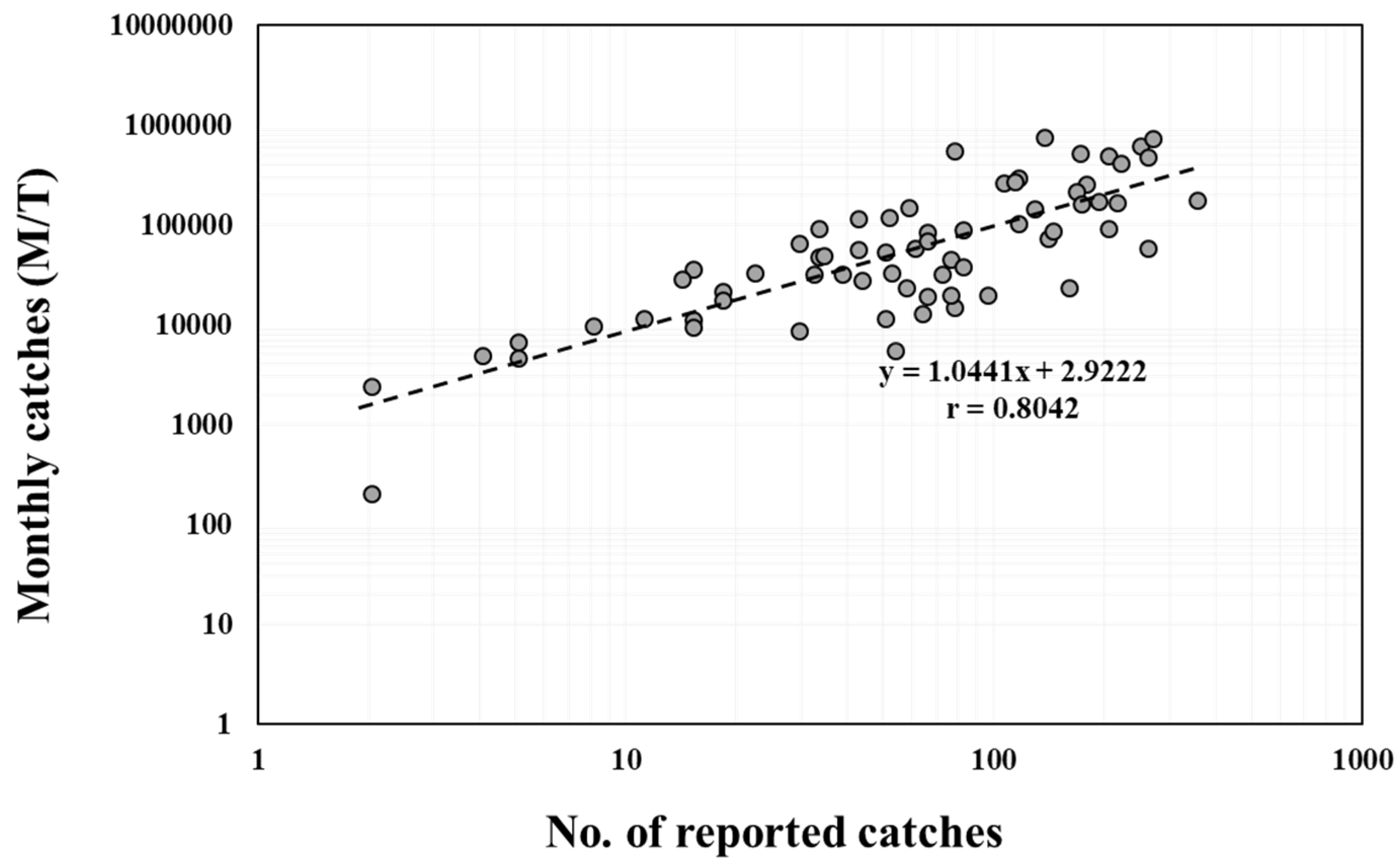
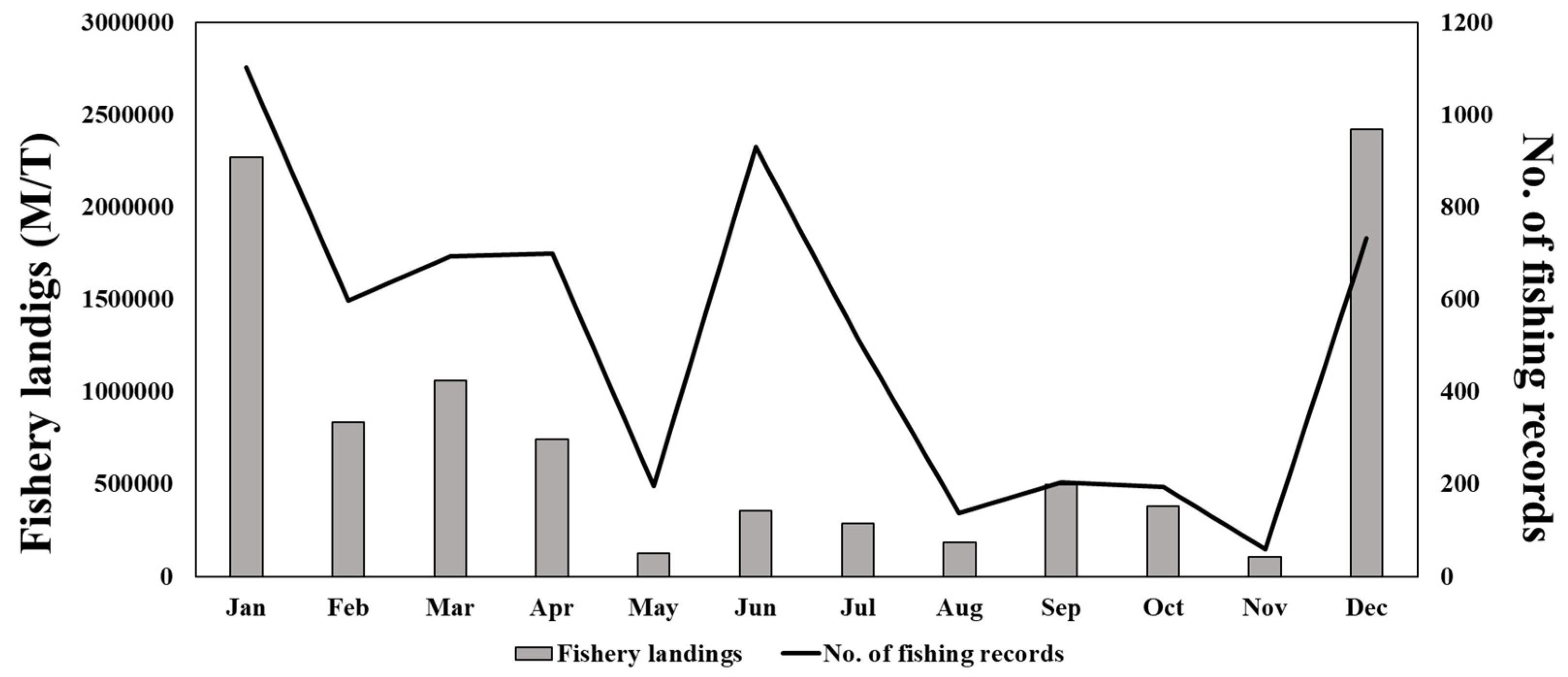
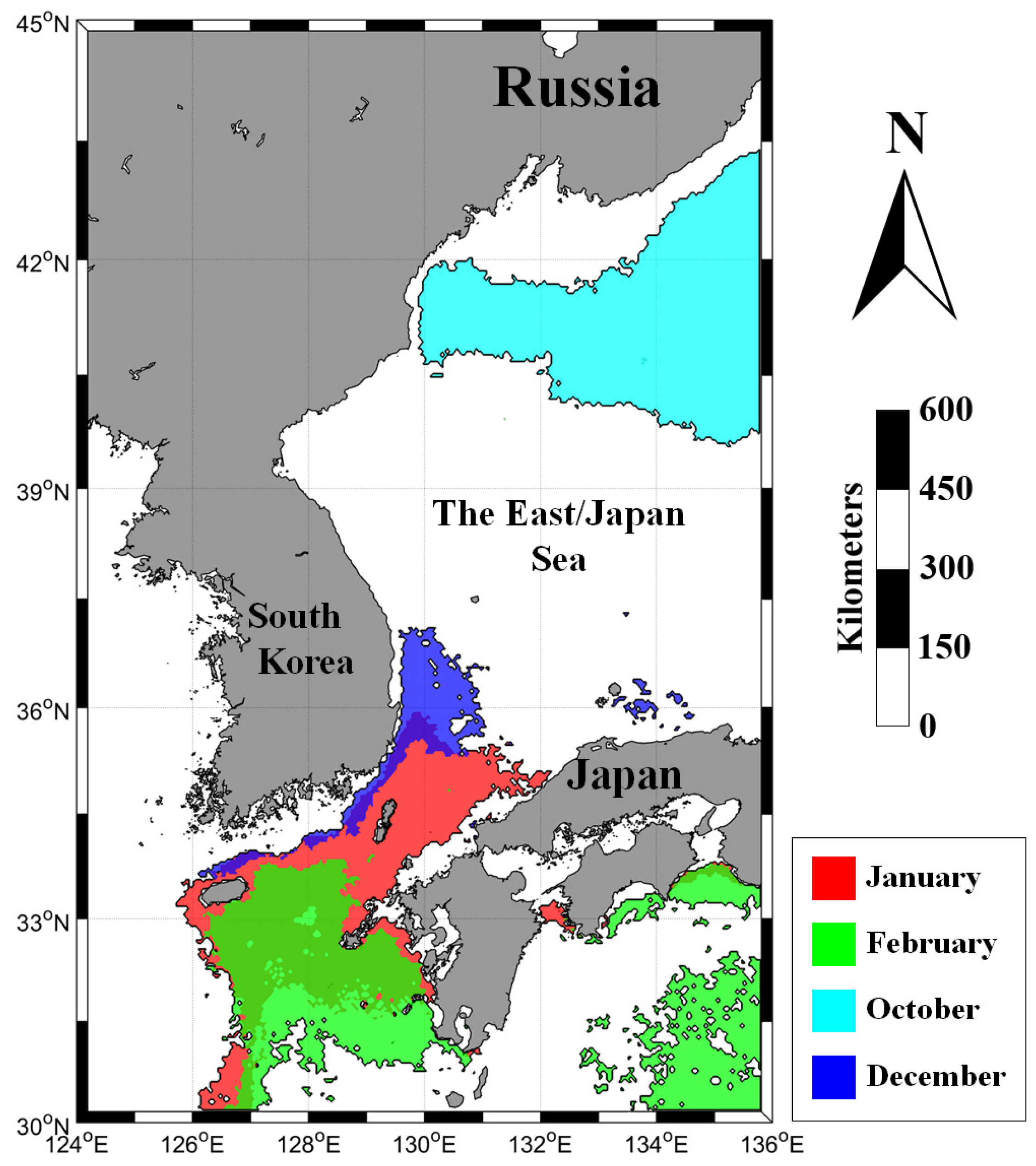
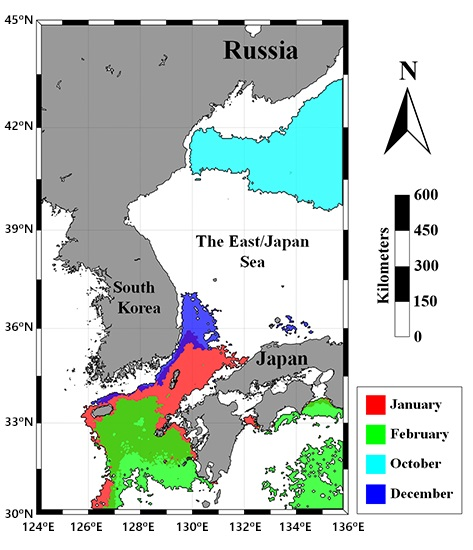
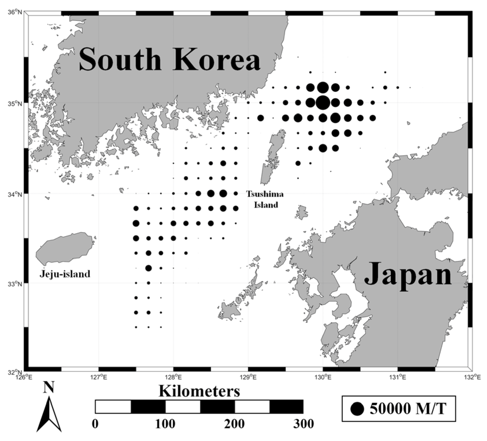
2.1. Fishery Data

The commercial catch data for chub mackerel in the South Sea from 2010 to 2016 were obtained from the Large Purse Seine Fishery Cooperatives of South Korea. The total number of reported catches was 6057, and these data include fishing locations and dates, as well as the amount of catch (M/T) (Figure 1). The fishing locations were collected at a spatial resolution of 0.17 degrees × 0.17 degrees (latitude × longitude).

2.2. Satellite Dataset

The satellite ocean color data from the Moderate Resolution Imaging Spectroradiometer (MODIS) on board the satellite Aqua platform provided by Ocean Biology Processing Group at NASA Goddard Space Flight Center (https://oceandata.sci.gsfc.nasa.gov/) were used for this study. MODIS Level-3 8-day composite data were obtained from July 2002 to December 2016 at 4-km of spatial resolution covering the South Sea and the East/Japan Sea.

The estimation of primary production from satellite ocean color data was performed with a regional algorithm based on the Vertically Generalized Productivity Model (VGPM) [22], described as:

$${\mathrm{PP}}_{\mathrm{eu}}=0.66125\times {\mathrm{P}}_{\mathrm{opt}}^B\times \left[{\mathrm{E}}_0{/\mathrm{E}}_0+4.1\right]{\times \mathrm{Z}}_{\mathrm{eu}}\times \mathrm{Chl}-a\times \mathrm{DL}$$

(1)

where PP_eu is the daily primary production integrated from surface to euphotic depth (mg C m⁻² d⁻¹), P^B_opt is the optimal carbon fixation rate (mg C (mg Chl)⁻¹ h⁻¹), E₀ is the amount of incident photosynthetically available radiation (PAR) during the day (E m⁻² d⁻¹), Z_eu is the euphotic depth (m), Chl-a is the concentration of chlorophyll-a (mg Chl m⁻²), and DL denotes photoperiod (h).

The P^B_opt is derived from the multiple regression equation with SST and Chl-a [23] as follows:

$${\mathrm{P}}_{\mathrm{opt}}^B=\frac{0.071\times \mathrm{SST}-3.2\times {10}^{-3}{\times \mathrm{SST}}^2+3.0\times {10}^{-5}\times {\mathrm{SST}}^3}{\mathrm{Chl}-a}+\left[1.0+0.17\times \mathrm{SST}-2.5\times {10}^{-3}\times {\mathrm{SST}}^2-8.0\times {10}^{-5}\times {\mathrm{SST}}^3\right]$$

(2)

2.3. Habitat Suitability Index Model

In previous studies, HSI models were derived from several environmental variables for a single species [13,15,24]. To judge habitat suitability, a suitability index (SI) is required for the environmental factors. Further, the suitability indices are combined into univariate variables. In this study, SST, Chl-a, and primary production (PP) were the selected environmental parameters to calculate HSI. It is well known that primary production is the major component of biological productivity, and hence, its role in habitats of marine fishes is significant.

The SIs for three parameters were calculated based on Chen et al. [13]. Each SI was estimated as a value between 0 and 1. The SIs were estimated by using the equation given below:

SI = exp(A × (X + B)²)

(3)

where, A and B are constants, and X is the values for the environmental parameters chosen.

It is possible to use several types of models, such as the Continued Product Model (CPM), Minimum Model (MINM), Arithmetic Mean Model (AMM), or Geometric Mean Model (GMM), when combining the SIs for the three variables [13,25,26,27,28,29]. However, several previous studies already reported that the AMM is the most appropriate model for the HSI of the chub mackerel [13,15,24]. Thus, the AMM was preferred for the present study and is described as below:

HSI = SI₁ × SI₂ × SI₃

(4)

To derive the HSI model, the number of fishing records rather than total catches were used; because fishing efforts were not true representatives for the amounts of the catches and population abundance. For example, there can be some cases where the amounts of the catches could be low although the environmental conditions of fishing favorable for the target species. On the other hand, fishing frequency data is considered to be more useful for the model approach due to the robustness and are less interfered by external effects relative to abundance data. The fishing records were calculated only when the fishing trip was completed successfully, but not for failed fishing. In addition to this, the relationship between the number of fishing records and the amount of catches in all different months was highly correlated (r = 0.8042, p < 0.001; Figure 2), and hence, the data on fishing records can be considered as being well representative of the amount of catch. For these reasons, the HSI algorithm used in this study was applied with the number of fishing records instead of the amount of catches.

3. Results

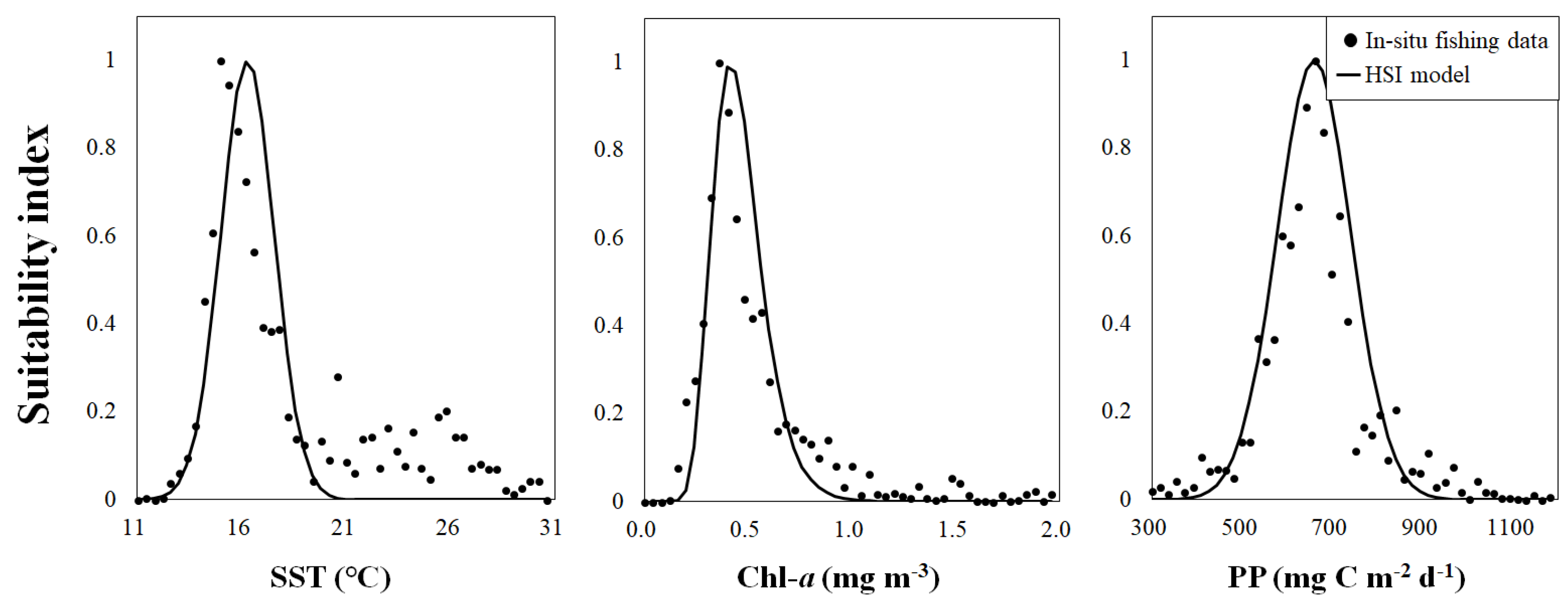
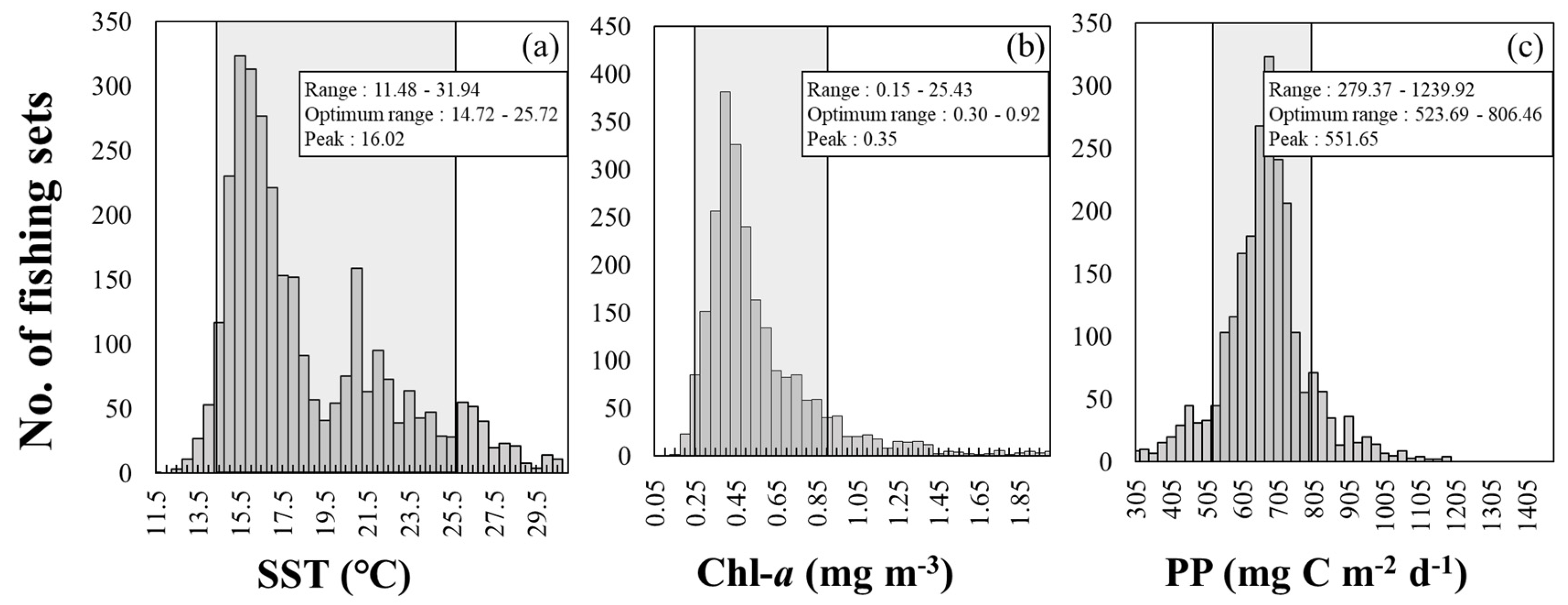
3.1. Preferred Environmental Conditions of the Chub Mackerel

To investigate the environmental conditions while fishing occurred, mean values in 3 × 3 pixels of each environmental parameter on every catch point from the satellite dataset were extracted. The number of catch data matched with the satellite dataset was 2309 (

Table 1. The number of commercial catch data matched with 8-day composited MODIS-Aqua datasets.

Year	Reported Catches	No. of Matchable Catches
2010	991	457
2012	789	336
2013	609	246
2014	809	277
2015	1715	586
2016	1144	407
Total	6057	2309

). Satellite data for many regions were unavailable due to cloudiness, and thus only approximately 38% of the catch data was matched with the satellite data. Although most of the catch data could not be used to derive an empirical relationship between the environmental factors and the chub mackerel catches, the remaining number of the catch data was enough to find the preferred habitat conditions for the chub mackerel in this study.

Monthly distributions of the number of fishing records and the amount of fishery landings showed a high seasonal dependency. The records suggest that more than half of the catches occurred from December to January (Figure 3).

The chub mackerel communities around South Korea were distributed under a wide range of environmental conditions. Our match-up results showed that these fish communities were distributed under SST conditions ranging from 11.48 to 31.94 °C, Chl-a from 0.15 to 25.43 mg m⁻³, and PP from 279.37 to 1239.92 mg C m⁻² d⁻¹ (Figure 4). Based on Kaschner et al. [30], the optimum ranges of the three parameters are defined as the 10th percentile and the 90th percentile of each parameter. The optimum ranges were defined as 14.72–25.72 °C, 0.30–0.92 mg m⁻³, and 523.69–806.46 mg C m⁻² d⁻¹ for SST, Chl-a, and PP, respectively. In the optimum conditions of SST, Chl-a and PP, the accounted for amounts of total catches were 81%, 86% and 82%, respectively.

3.2. Habitat Suitability Index Model Derivation

To derive the HSI values for the chub mackerel, three empirical models were used (

Table 2. Suitability index (SI) models derived from three environmental parameters (SST, Chl-a, and PP).

Variables	SI Models	RMSE	R2
SST	exp (−0.3034(XSST − 16.3)2)	0.1440	0.6480
Chl-a	exp(−6.963(ln(XChl) + 0.8782)2)	0.0478	0.9325
PP	exp(−0.00007347(XPP − 659.3)2)	0.1211	0.8253

). The SI models for the environmental parameters were adapted from Chen et al. [13]. The constants of the models were obtained from the least squares fitting to derive optimized models for the study area (Figure 5). In the case of Chl-a, a natural logarithmic form to fit to the asymmetric distribution of the Chl-a concentration was used. The logarithmic form was not applied for SST, though, since SST can also have a negative value in cold environments.

The RMSE of the SI models for SST, Chl-a, and PP were 0.1440, 0.0478, and 0.1211, respectively. The coefficients of determination (R²) for the SI models were 0.65, 0.93, and 0.83 for SST, Chl-a, and PP, respectively.

The climatological monthly distribution (July 2002–December 2016) of the HSI by the AMM model showed that a high HSI was observed in the southern coastal sea of South Korea from winter to early spring and then appeared in the East/Japan Sea from late spring to fall (Figure 6).

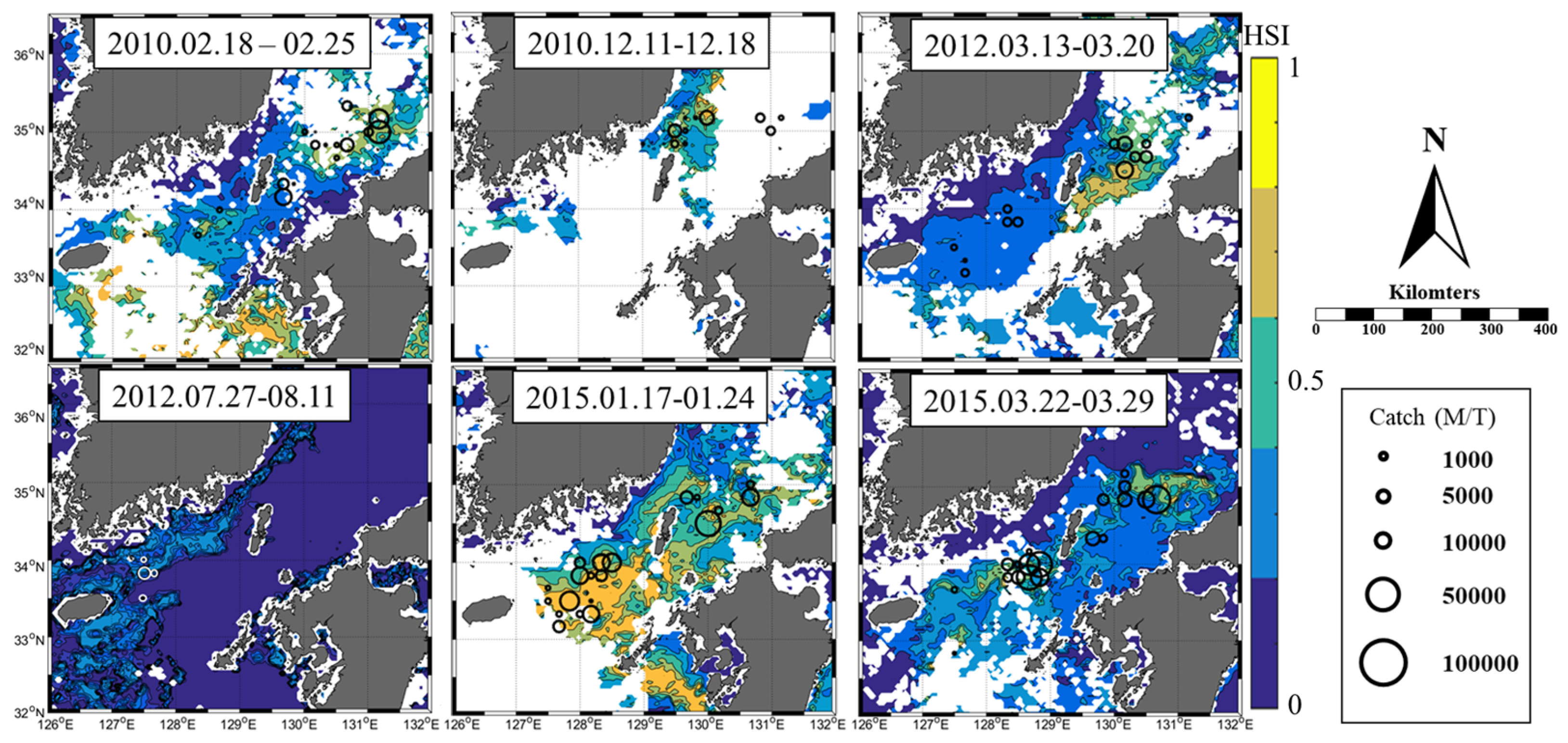
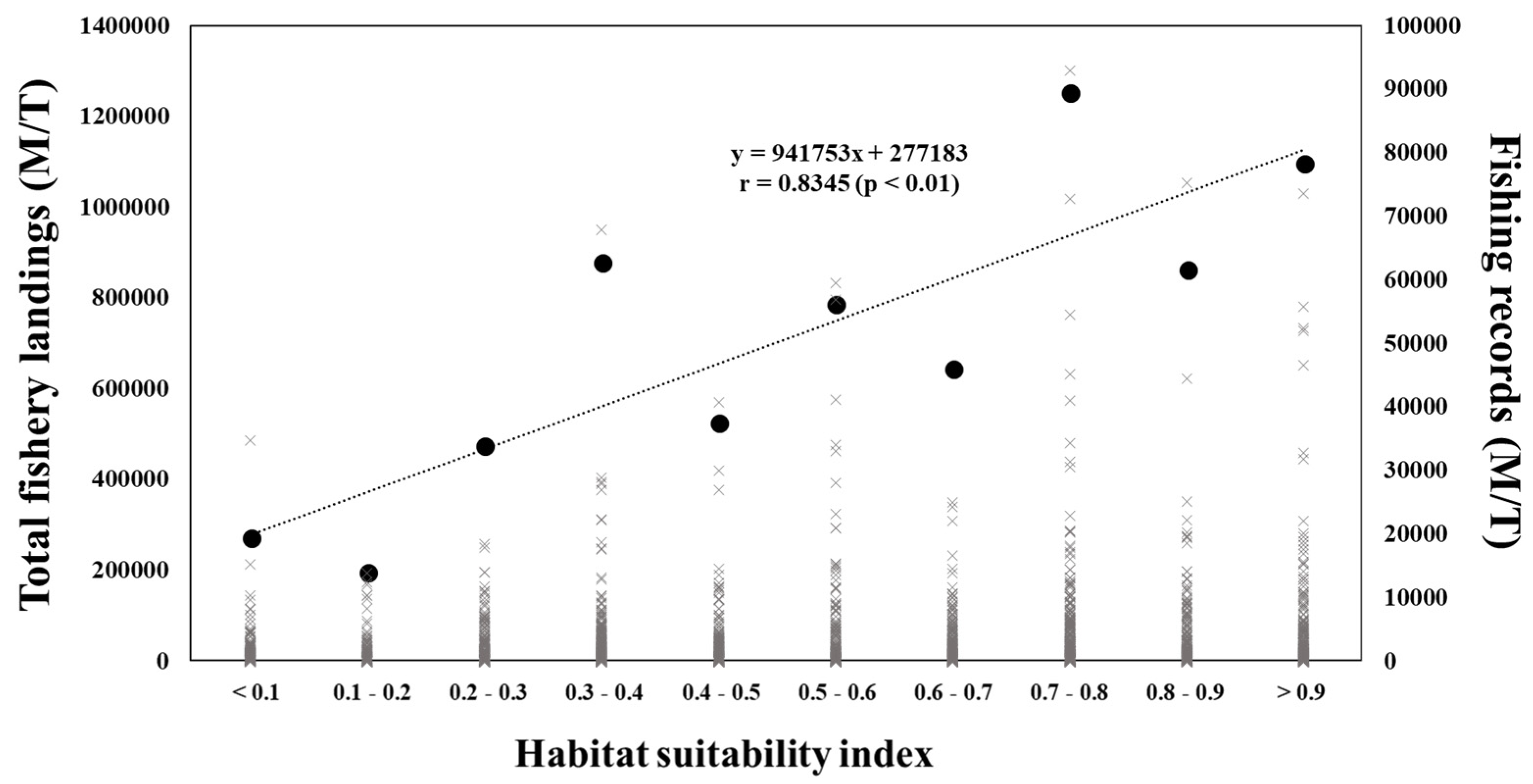
3.3. Habitat Suitability Index Model Evaluation

To validate our HSI model, the HSI values from our model were compared with fishery catches. The HSIs were divided into 10 classes with an equal interval of 0.1. Then, the landed fisheries from the region with the HSI values corresponding to each class were summed. A strong positive linear relationship (r = 0.83) was observed between the HSI and the fishery landings (Figure 7). In addition to that, spatial distributions between the HSIs and the fish catches for the chub mackerel were observed to have a significant correlation throughout the study period from 2010 to 2016 (Figure 8).

4. Discussion

4.1. Environmental Factors Affecting the Chub Mackerel

In general, spatial and temporal distributions of marine fish are largely influenced by SST and salinity [31,32,33]. In many previous studies, optimal conditions for the chub mackerel have been reported for SST, salinity, and Chl-a concentration [13,15,30]. However, salinity was not considered in this study, since its variation in the East/Japan Sea and the South Sea mostly fell within the reported optimal ranges (from 31.90 to 35.16) [20] for the chub mackerel. Instead, we tried to examine the optimal conditions for the chub mackerel with other environmental variables.

Although the chub mackerel is not a direct predator of phytoplankton, intermediate trophic levels in the food web are strongly influenced by phytoplankton distribution [34]. Indeed, Lee et al. [35] reported that the spatial distribution of the common minke whale (Balaenoptera acutorostrata) is highly associated with the Chl-a distribution in the East/Japan Sea [35], even though there is not any direct linkage between the minke whale and phytoplankton in the food web. Generally, zooplankton play a major role in the food web as grazers and are closely related to the distribution of phytoplankton [34]. Zooplankton communities are not only a main prey for the juvenile chub mackerel, but also for the small pelagic fishes which are the main food for the adult chub mackerel. Such indirect relationships between phytoplankton communities and the chub mackerel species allow us to estimate relative abundance of the chub mackerel under various environmental conditions, which are crucial for primary producers too. Thus, phytoplankton-related parameters, such as Chl-a concentration and PP, can be significant tracers for the spatial and temporal distribution of the chub mackerel. Although PP is related with Chl-a, they do not always show a consistent positive relationship, because PP is also strongly dependent on many other parameters, such as photosynthetically available radiation (PAR), diffuse attenuation coefficient (K_d), day length, etc. As shown in Joo et al. [36], spring phytoplankton bloom (i.e., maximum Chl-a) in the East/Japan Sea usually appears during April; however, the maximum PP is obtained during May and June [36]. In addition to this, the lowest Chl-a usually appears during the summer months, whereas PP becomes the lowest during the winter months, when light is limited.

The modified VGPM algorithm used in this study represented the primary production in the entire euphotic depth, while Chl-a data were acquired in near surface waters. Because the chub mackerel’s habitat depth is not near-surface, the consideration of PP could improve the algorithm’s performance. In this study, a significant relationship between the HSIs, including PP parameters and fishery landings, was observed (Figure 7).

On the other hand, fitting the results of suitability index models showed an inaccuracy in areas with environmental ranges beyond optimal conditions. There are gaps between the SI models and the in situ dataset, especially in the SI model for the SST (Figure 5). This suggests that the HSI can be underestimated in low HSI regions. However, no sign of an underestimated HSI was found in this study.

The optimal environmental conditions for the chub mackerel in this study showed similar results with Species Environmental Envelope (HSPEN) in AquaMaps global distribution model [30]. The species’ preferred conditions for the chub mackerel in AquaMaps are 12.74–27.88 °C and 214–1800 mg C m⁻² d⁻¹ for temperature and PP, respectively [30], which correspond well with the results from our study. The optimal environmental conditions for the Atlantic chub mackerel (Scomber colias) and blue mackerel (Scomber australasicus) also showed similar ranges to the results from this study. However, the optimal conditions for the chub mackerel reported by Chen et al. [13] were substantially different (28–29.4 °C and 0.15–0.50 mg m⁻³ for SST and Chl-a, respectively) from our results (14.72–25.72 °C and 0.30–0.92 mg m³). This inconsistency in the range could be due to the differences in the seasonal distribution of catches due to different target areas. The chub mackerel in the East China Sea is subjected to a large scale commercial exploitation from July to September. However, the results from the present study indicate that the chub mackerel in the South Sea are mainly exploited from December to January [13]. This implies that the favored environmental conditions for the chub mackerel could be seasonally different, and thus the monitoring or the management strategy for the population should be established on a seasonal basis.

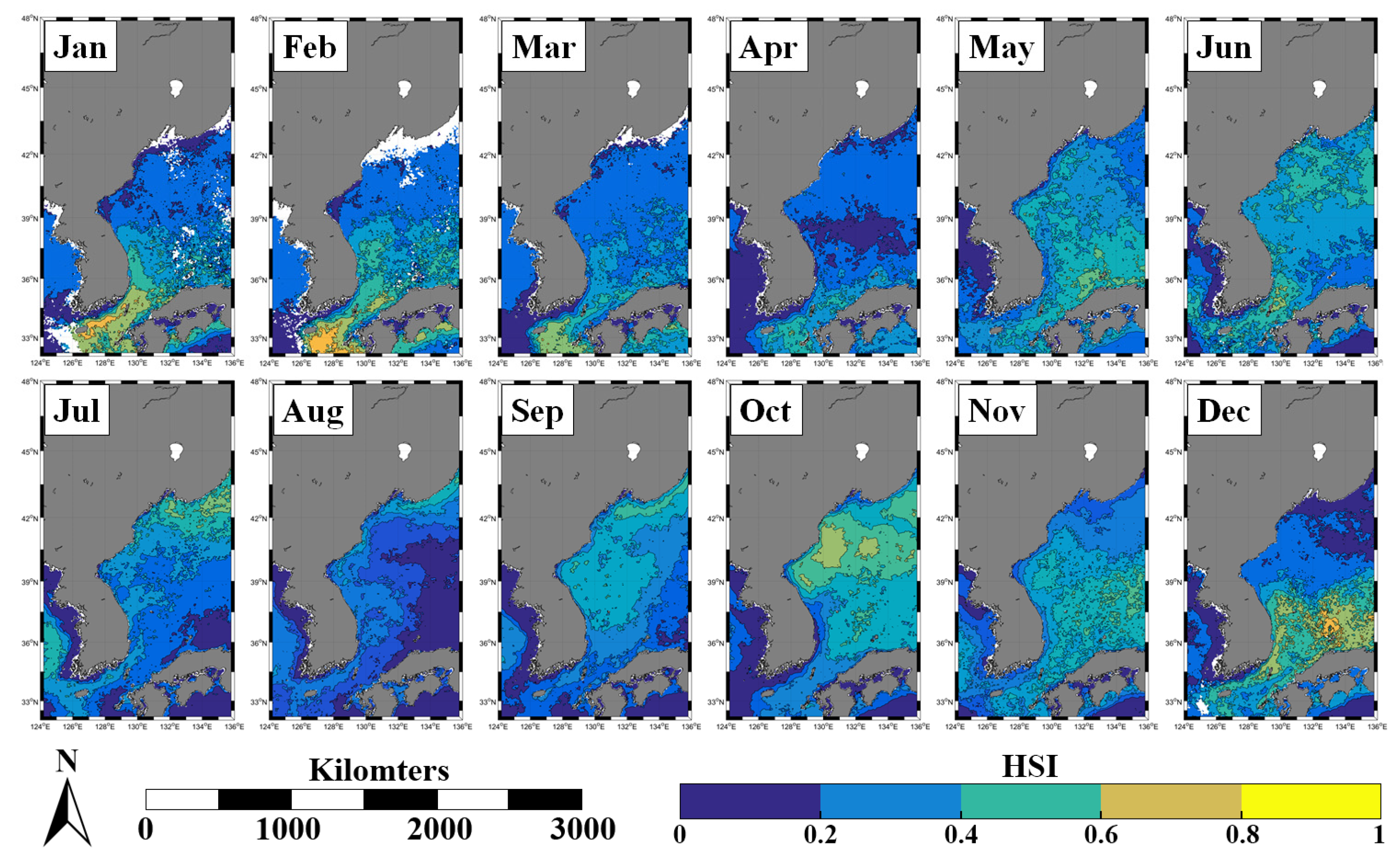
4.2. Seasonal Distribution of the HSI

The climatological monthly analysis from 2002 to 2016 showed seasonal variations in the distribution of the HSIs for the chub mackerel (Figure 6). During the middle of winter, a high HSI region was formed in the South Sea. Then, during late spring, the HSI in the South Sea was observed to be declined, and further, the high HSI region showed a northward movement to the East/Japan Sea. After the fall season, the high HSI area started to move back to the south. Indeed, the South Sea is well known as the wintering and spawning ground of the chub mackerel inhabiting the waters around the Korean Peninsula [6,7]. The spawning of the chub mackerel occurs mainly during spring [37]. After the spawning season, the chub mackerel migrate to the East/Japan Sea, which is known to be their feeding ground, and their feeding activity generally continues until November. Then, they return back to the wintering ground in the South Sea [5]. Consequently, the general migration pattern of the chub mackerel in Korean waters was well reflected in the HSI results from the present study. Therefore, the preferred environmental conditions for the chub mackerel could be predicted well with the HSI model in this study.

4.3. Hotspot Analysis of the HSI

For the investigation of the HSI hotspots for the chub mackerel, the proportion of landed fisheries for each HSI range was estimated. The results suggested that more than half of the catches occurred in areas when the HSIs ranged to 0.6 or more. Thus, the assumption was made that hotspots for the chub mackerel occur in regions with HSI > 0.6. The definition of a hotspot in this study means that the environmental conditions in the region are suitable to chub mackerel’s preferences, and thus chub mackerel communities are more likely to be found around these spots. Based on this assumption, the hotspots from the climatological distribution of the HSI were analyzed.

The results of our hotspot analysis showed three hotspots of the HSI in the East/Japan Sea and the South Sea (Figure 9). One hotspot is observed in the South Sea during the winter season. Because of good environmental conditions, the spawning and wintering ground for the chub mackerel is generally formed in the South Sea [6,7], which is consistent with our high HSI during the winter in that area (Figure 9). The South Sea is an important region for the chub mackerel where the population of this species coming from the North Pacific Ocean usually divides into two subpopulations, the Tsushima Current population in the East/Japan Sea and the Yellow Sea population [14]. Another hotspot is located near Okinoshima, Japan, and is mostly observed in December (Figure 9). This hotspot region is also known as a spawning and wintering ground for the chub mackerel [3,14]. Based on these results, the population of the chub mackerel in the East/Japan Sea can be divided into at least two subpopulations. Indeed, many fishing activities are carried out in the East/Japan Sea hotspot in December, according to the logbooks of the Japan Sea purse seine fisheries [38], although the South Sea hotspot is also a major fishing ground for the chub mackerel.

In October, a large hotspot is found in the northern part of the East/Japan Sea. While the chub mackerel migrates northward of the East/Japan Sea, they usually branch off to several pathways [39]. Once they reach the northernmost part of their migration route during autumn, they start to move southward. It is possible for them to take several pathways while they migrate southward; however, the point where all the paths intersect is usually located near the Peter the Great Bay, Russia [38]. These various migration routes for the chub mackerel are well reflected in the wide hotspot that appeared in the north of the East/Japan Sea in October (Figure 9).

5. Summary and Conclusions

In this study, the HSI of the chub mackerel (Scomber japonicus) was derived by using commercial catch data and MODIS-Aqua satellite datasets between 2010 and 2016. Three environmental parameters (SST, Chl-a, and PP) were selected as key variables in the habitat formation of the chub mackerel in the South Sea of South Korea. The optimum ranges were 14.72–25.72 °C, 0.30–0.92 mg m⁻³, and 523.69–806.46 mg C m⁻² d⁻¹ for SST, Chl-a, and PP, respectively (Figure 4). More than 80% of the total catch obtained from the region within the optimum ranges. In the derivation of the HSI model, the AMM was used to combine the three SIs (SST, Chl-a, and PP) since many previous studies reported that the AMM is the most appropriate model for marine fish species.

Based on the results from the HSI model, a strong positive relationship (r = 0.83) between the HSI and the fishery landings (Figure 7) and a good match for the spatial distributions of the chub mackerel were found (Figure 8). The seasonal northward and southward movements of a high HSI region were observed in climatological monthly distribution of the HSI (Figure 6). The high HSI area observed in the South Sea during winter time was observed to move northward during late spring. After the fall season, the high HSI area was observed to be moving back towards the southern part of Korean waters. In addition to this, the hotspot analysis revealed that there were three major hotspots in the South Sea and the East/Japan Sea during from 2002 to 2016 (Figure 9). The hotspots observed in the South Sea and the southern East/Japan Sea were consistent with the reported wintering and spawning grounds for the chub mackerel. The hotspot observed in the northern East/Japan Sea during October could be related to various migration routes for the chub mackerel. Consequently, the seasonal and spatial variations of the HSI were in agreement with the migration patterns of the chub mackerel reported previously in the South Sea and East/Japan Sea. The HSI model derived from the present study is capable of giving sufficient information to predict fishing grounds of the chub mackerel around South Korea.

References

1. Collette, B.B.; Nauen, C.E. FAO Species Catalogue. Volume 2. Scombrids of the World. An Annotated and Illustrated Catalogue of Tunas, Mackerels, Bonitos and Related Species Known to Date; FAO: Rome, Italy, 1983. [Google Scholar]
2. Kiparissis, S.; Tserpes, G.; Tsimenidis, N. Aspects on the Demography of Chub Mackerel (Scomber japonicus Houttuyn, 1782) in the Hellenic Seas. Belg. J. Zool. 2000, 130, 3–7. [Google Scholar]
3. Hwang, S.; Kim, J.; Lee, T. Age, Growth, and Maturity of Chub Mackerel off Korea. N. Am. J. Fish. Manag. 2008, 28, 1414–1425. [Google Scholar] [CrossRef]
4. Korea, S.; Korean Statistical Information Service (KOSIS). Fishery Production Survey; Korean Statistical Information Service (KOSIS): Daejeon, Korea, 2017. [Google Scholar]
5. Choi, Y.; Zhang, C.; Lee, J.; Kim, J.; Cha, H. Stock Assessment and Management Implications of Chub Mackerel, Scomber japonicus in Korean Waters; Pukyong National University: Busan, Korea, 2003; pp. 10–13. [Google Scholar]
6. Chyung, M. The Fishes of Korea; Il Ji Sa: Seoul, Korea, 1977. [Google Scholar]
7. Yoon, S.; Kim, D.; Baeck, G.; Kim, J. Feeding Habits of Chub Mackerel (Scomber japonicus) in the South Sea of Korea. Korean J. Fish. Aquat. Sci. 2008, 41, 26–31. [Google Scholar] [CrossRef]
8. NFRDI (National Fisheries Research and Development Institute). Ecology and Fishing Grounds for Some Major Fish in Korean Waters; National Fisheries Research and Development Institute: Busan, Korea, 2005.
9. Parmesan, C.; Yohe, G. A Globally Coherent Fingerprint of Climate Change Impacts across Natural Systems. Nature 2003, 421, 37–42. [Google Scholar] [CrossRef] [PubMed]
10. Perry, A.L.; Low, P.J.; Ellis, J.R.; Reynolds, J.D. Climate Change and Distribution Shifts in Marine Fishes. Science 2005, 308, 1912–1915. [Google Scholar] [CrossRef] [PubMed] [Green Version]
11. Daskalov, G.M.; Grishin, A.N.; Rodionov, S.; Mihneva, V. Trophic Cascades Triggered by Overfishing Reveal Possible Mechanisms of Ecosystem Regime Shifts. Proc. Natl. Acad. Sci. USA 2007, 104, 10518–10523. [Google Scholar] [CrossRef] [PubMed]
12. Jones, D.D.; Walters, C.J. Catastrophe Theory and Fisheries Regulation. J. Fish. Board Can. 1976, 33, 2829–2833. [Google Scholar] [CrossRef]
13. Chen, X.; Li, G.; Feng, B.; Tian, S. Habitat Suitability Index of Chub Mackerel (Scomber japonicus) from July to September in the East China Sea. J. Oceanogr. 2009, 65, 93–102. [Google Scholar] [CrossRef]
14. Hiyama, Y.; Yoda, M.; Ohshimo, S. Stock Size Fluctuations in Chub Mackerel (Scomber japonicus) in the East China Sea and the Japan/East Sea. Fish. Oceanogr. 2002, 11, 347–353. [Google Scholar] [CrossRef]
15. Li, G.; Chen, X.; Lei, L.; Guan, W. Distribution of Hotspots of Chub Mackerel Based on Remote-Sensing Data in Coastal Waters of China. Int. J. Remote Sens. 2014, 35, 4399–4421. [Google Scholar] [CrossRef]
16. Zheng, B.; Chen, X.; Li, G. Relationship between the Resource and Fishing Ground of Mackerel and Environmental Factors Based on GAM and GLM Models in the East China Sea and Yellow Sea. J. Fish. China 2008, 3, 007. [Google Scholar]
17. Brooks, R.P. Improving Habitat Suitability Index Models. Wildl. Soc. Bull. (1973–2006) 1997, 25, 163–167. [Google Scholar]
18. Galparsoro, I.; Borja, Á.; Bald, J.; Liria, P.; Chust, G. Predicting Suitable Habitat for the European Lobster (Homarus gammarus), on the Basque Continental Shelf (Bay of Biscay), using Ecological-Niche Factor Analysis. Ecol. Model. 2009, 220, 556–567. [Google Scholar] [CrossRef]
19. Morris, L.; Ball, D. Habitat Suitability Modelling of Economically Important Fish Species with Commercial Fisheries Data. ICES J. Mar. Sci. 2006, 63, 1590–1603. [Google Scholar] [CrossRef]
20. Rubec, P.J.; Bexley, J.C.; Norris, H.; Coyne, M.S.; Monaco, M.E.; Smith, S.G.; Ault, J.S. Suitability Modeling to Delineate Habitat Essential. In American Fisheries Society Symposium 22; American Fisheries Society: Bethesda, MD, USA, 1999; pp. 108–133. [Google Scholar]
21. Vinagre, C.; Fonseca, V.; Cabral, H.; Costa, M.J. Habitat Suitability Index Models for the Juvenile Soles, Solea solea and Solea senegalensis, in the Tagus Estuary: Defining Variables for Species Management. Fish. Res. 2006, 82, 140–149. [Google Scholar] [CrossRef]
22. Behrenfeld, M.J.; Falkowski, P.G. Photosynthetic Rates Derived from satellite-based Chlorophyll Concentration. Limnol. Oceanogr. 1997, 42, 1–20. [Google Scholar] [CrossRef]
23. Yamada, K.; Ishizaka, J.; Nagata, H. Spatial and Temporal Variability of Satellite Primary Production in the Japan Sea from 1998 to 2002. J. Oceanogr. 2005, 61, 857–869. [Google Scholar] [CrossRef]
24. Yen, K.; Lu, H.; Chang, Y.; Lee, M. Using Remote-Sensing Data to Detect Habitat Suitability for Yellowfin Tuna in the Western and Central Pacific Ocean. Int. J. Remote Sens. 2012, 33, 7507–7522. [Google Scholar] [CrossRef]
25. Chen, X.; Feng, B.; Xu, L. A Comparative Study on Habitat Suitability Index of Bigeye Tuna, Thunnus obesus in the Indian Ocean. J. Fish. Sci. China 2008, 15, 269–278. [Google Scholar]
26. Grebenkov, A.; Lukashevich, A.; Linkov, I.; Kapustka, L.A. A habitat suitability evaluation technique and its application to environmental risk assessment. In Ecotoxicology, Ecological Risk Assessment and Multiple Stressors; Springer: Berlin/Heidelberg, Germany, 2006; pp. 191–201. [Google Scholar]
27. Hess, G.R.; Bay, J.M. A Regional Assessment of Windbreak Habitat Suitability. Environ. Monit. Assess. 2000, 61, 239–256. [Google Scholar] [CrossRef]
28. Lauver, C.L.; Busby, W.H.; Whistler, J.L. Testing a GIS Model of Habitat Suitability for a Declining Grassland Bird. Environ. Manag. 2002, 30, 88–97. [Google Scholar] [CrossRef] [PubMed]
29. Van der Lee, G.E.M.; Van der Molen, D.T.; Van den Boogaard, H.F.P.; Van der Klis, H. Uncertainty Analysis of a Spatial Habitat Suitability Model and Implications for Ecological Management of Water Bodies. Landsc. Ecol. 2006, 21, 1019–1032. [Google Scholar] [CrossRef]
30. Kaschner, K.; Kesner-Reyes, K.; Garilao, C.; Rius-Barile, J.; Rees, T.; Froese, R. AquaMaps: Predicted Range Maps for Aquatic Species. World Wide Web Electronic Publication Version 08/2016. Available online: www.aquamaps.org (accessed on 3 April 2018).
31. Castillo, J.; Barbieri, M.; Gonzalez, A. Relationships between Sea Surface Temperature, Salinity, and Pelagic Fish Distribution off Northern Chile. ICES J. Mar. Sci. 1996, 53, 139–146. [Google Scholar] [CrossRef]
32. Jaureguizar, A.J.; Menni, R.; Guerrero, R.; Lasta, C. Environmental Factors Structuring Fish Communities of the Rıo de la Plata Estuary. Fish. Res. 2004, 66, 195–211. [Google Scholar] [CrossRef]
33. Sutcliffe, W., Jr.; Drinkwater, K.; Muir, B. Correlations of Fish Catch and Environmental Factors in the Gulf of Maine. J. Fish. Board Can. 1977, 34, 19–30. [Google Scholar] [CrossRef]
34. Smith, R.; Dustan, P.; Au, D.; Baker, K.; Dunlap, E. Distribution of Cetaceans and Sea-Surface Chlorophyll Concentrations in the California Current. Mar. Biol. 1986, 91, 385–402. [Google Scholar] [CrossRef]
35. Lee, D.; An, Y.R.; Park, K.J.; Kim, H.W.; Lee, D.; Joo, H.T.; Oh, Y.G.; Kim, S.M.; Kang, C.K.; Lee, S.H. Spatial Distribution of Common Minke Whale (Balaenoptera acutorostrata) as an Indication of a Biological Hotspot in the East Sea. Deep Sea Res. Part II 2017, 143, 91–99. [Google Scholar] [CrossRef]
36. Joo, H.T.; Son, S.; Park, J.W.; Kang, J.J.; Jeong, J.Y.; Lee, C.I.; Kang, C.K.; Lee, S.H. Long-Term Pattern of Primary Productivity in the East/Japan Sea Based on Ocean Color Data Derived from MODIS-Aqua. Remote Sens. 2016, 8, 25. [Google Scholar] [CrossRef]
37. Cha, H.; Choi, Y.; Park, J.; Kim, J.; Sohn, M. Maturation and Spawning of the Chub Mackerel, Scomber japonicus Houttuyn in Korean Waters. J. Korean Soc. Fish. Res. 2002, 5, 24–33. [Google Scholar]
38. Yasuda, T.; Yukami, R.; Ohshimo, S. Fishing Ground Hotspots Reveal Long-Term Variation in Chub Mackerel Scomber japonicus Habitat in the East China Sea. Mar. Ecol. Prog. Ser. 2014, 501, 239–250. [Google Scholar] [CrossRef]
39. Nishimura, S. The Zoogeographical Aspects of the Japan Sea—Part II. Publ. Seto Mar. Biol. Lab. 1965, 13, 81–101. [Google Scholar] [CrossRef] [Green Version]
Figure 1. Summarized commercial catch data for the chub mackerel from 2010 to 2016.
Remotesensing 10 00938 g001
Figure 2. Correlation between logarithmic monthly catches and amount of reported catches (n = 67).
Remotesensing 10 00938 g002
Figure 3. Monthly distribution of total fishery landings (M/T) and the number of fishing records.
Remotesensing 10 00938 g003
Figure 4. Frequency distributions of (a) Sea surface temperature (SST; °C), (b) Chlorophyll-a (Chl-a; mg m−3), and (c) Primary production (PP; mg C m−2 d−1) on the fishing locations for the chub mackerel. Gray squares represent the optimum ranges for each parameter.
Remotesensing 10 00938 g004
Figure 5. Least squares fitting results of (a) SST (°C), (b) Chl-a (mg m−3), and (c) PP (mg C m−2 d−1) with the number of fishing sets (solid line: habitat suitability index (HSI) model, black dot: in situ fishing data).
Remotesensing 10 00938 g005
Figure 6. Climatological monthly distribution of the HSI around South Korea from 2002 to 2016.
Remotesensing 10 00938 g006
Figure 7. Distribution of fishing records in each range of HSI (gray cross) and the total fishery landings (black dot). Total fishery landings are summed catches in each range of the HSI value. Black line represents the correlation between total fishery landings and HSIs.
Remotesensing 10 00938 g007
Figure 8. Spatial distribution of the 8-day composited HSI and the chub mackerel catches at corresponding periods in the South Sea.
Remotesensing 10 00938 g008
Figure 9. The HSI hotspots for the chub mackerel observed in the South Sea and the East/Japan Sea.
Remotesensing 10 00938 g009