Land Cover Segmentation of Airborne LiDAR Data Using Stochastic Atrous Network


1
Faculty of Science and Technology, Norwegian University of Life Sciences, 1432 Ås, Norway
2
Division of Survey and Statistics, Norwegian Institute of Bioeconomy Research, 1431 Ås, Norway
*
Author to whom correspondence should be addressed.
Remote Sens. 2018, 10(6), 973; https://doi.org/10.3390/rs10060973
Submission received: 30 April 2018
/
Revised: 15 June 2018
/
Accepted: 17 June 2018
/
Published: 19 June 2018
(This article belongs to the Special Issue Deep Learning for Remote Sensing)
Abstract
:Inspired by the success of deep learning techniques in dense-label prediction and the increasing availability of high precision airborne light detection and ranging (LiDAR) data, we present a research process that compares a collection of well-proven semantic segmentation architectures based on the deep learning approach. Our investigation concludes with the proposition of some novel deep learning architectures for generating detailed land resource maps by employing a semantic segmentation approach. The contribution of our work is threefold. (1) First, we implement the multiclass version of the intersection-over-union (IoU) loss function that contributes to handling highly imbalanced datasets and preventing overfitting. (2) Thereafter, we propose a novel deep learning architecture integrating the deep atrous network architecture with the stochastic depth approach for speeding up the learning process, and impose a regularization effect. (3) Finally, we introduce an early fusion deep layer that combines image-based and LiDAR-derived features. In a benchmark study carried out using the Follo 2014 LiDAR data and the NIBIO AR5 land resources dataset, we compare our proposals to other deep learning architectures. A quantitative comparison shows that our best proposal provides more than 5% relative improvement in terms of mean intersection-over-union over the atrous network, providing a basis for a more frequent and improved use of LiDAR data for automatic land cover segmentation.
1. Introduction
The advancement of airborne LiDAR (light detection and ranging) technologies over the past decades have contributed significantly to the increased availability of high precision point cloud data. Thanks to the government project “Nasjonal detaljert høydemodell” [1], LiDAR data are already available for many parts of Norway through the “høydedata” website [2]. The aim of the project is to provide national coverage of high-resolution elevation data by 2019.
Easy access to high-precision LiDAR data in Norway opens an opportunity to identify and extract valuable information for many different purposes. Airborne LiDAR data have become the basis for generating a high accuracy digital terrain model, hazard assessment and susceptibility mapping, and the monitoring of surface displacements [3]. In terms of land cover classification, LiDAR data have been used to automatically generate maps for forest fire management [4] and land/water classification [5]. However, due to the complexity of the data and the difficulty of generating features of interest, most of the current techniques suffer from scaling problems when transferred to larger datasets [6].
We have investigated deep learning techniques to create a classifier for the AR5 land resource dataset [7] from Norwegian Institute of Bioeconomy Research (NIBIO). AR5 is the national high-resolution, combined land cover and land capability dataset for Norway. Challenges with this dataset include: (a) AR5, as “ground truth” data, is an imperfect match with our LiDAR data due to the difference in resolution/level of detail; (b) the different generalization approaches and data sources that have been used to generate the AR5 classes; (c) differences in the acquisition times of AR5 and the LiDAR data; (d) point cloud data are represented as points in a specified location, which requires a fine-grain preprocessing technique to make them usable in a semantic segmentation pipeline.
One of the most common techniques for doing land cover segmentation is by engineering handcrafted features from the LiDAR data to train a machine learning algorithm for automatic detection. Guo et al. investigates 26 manually derived features from LiDAR data for the purpose of automatic classification [8], while MacFaden et al. utilizes normalized difference vegetation index (NDVI), normalized digital surface model (nDSM), and high-resolution multispectral images to do high-resolution tree canopy mapping for the same purpose [9]. Yan et al. [10] reviews a number of research projects that utilize LiDAR data for automated extraction, using three LiDAR-derived features for generating urban land cover maps [11] to several full waveform-derived features for the classification of dense urban scenes [12].
The manual engineering of features as inputs to a machine learning classifier has become common practice for generating land segmentation maps [8,9,10,11,12]. However, such approaches limit the ability to provide a richer representation of the data [13]. The chosen features may not be sufficient to characterize the uniqueness of a certain class or object [14], and the quality of the resulting classifier depends heavily on the feature engineering output. As each particular segmentation problem is more or less unique [15], different feature engineering approaches are often needed for different problems.
Deep learning methodologies contribute to simplifying the feature engineering process, and by using a deep multi-layer convolutional neural network (CNN) [16], the features are learned from the data during the training process. Consequently, a successfully trained CNN model can be considered as a feature extractor that both combines features in different spatial locations and takes into account the aspects of spatial autocorrelation between features.
From the era of AlexNet [17] in 2012 to the more complex deep learning architectures such as GoogleNet [18] and ResNet [19] in 2014 and 2015, respectively, deep learning has become one of the most successful machine learning techniques for approaching problems related to computer vision, including image classification, object detection, and more advanced challenges such as semantic segmentation and instance-aware segmentation. In the remote sensing community, deep learning has also been used successfully for land cover classification [20], road detection [21], and scene understanding [22].
The purpose of the present paper is to investigate and compare a collection of well-proven semantic segmentation architectures based on the deep learning approach. Based on the experiences obtained from this investigation, we propose a novel deep learning architecture for the particular land cover segmentation problem of interest. The proposed architecture involves a CNN fusion layer for merging the image-based features with height above ground information and intensity values. The output of the fusion layer provides the basis for training an atrous deep network [23] using the stochastic depth approach [24] combined with a rescaling of the derived feature map using skip connections and the learnable upsampling approach, which is similar to the technique in fully convolutional networks [25]. The final layer of our architecture includes a softmax activation function combined with an intersection-over-union (IoU) loss function [26] that both speed up the convergence process and improve the accuracy of the resulting classifier. We are able to demonstrate that the classifier resulting from our proposed architecture gains more than 5% accuracy improvement (validated) over the atrous network (DeeplabV2) [23].
In the next section, we review some of the most popular deep learning techniques for semantic segmentation. In the subsequent sections, we describe the characteristics and properties of our datasets, and the challenges that come with them. Thereafter, we report the results of our research process, where we explore some of the most well-proven deep learning architectures for semantic segmentation. Based on our findings, we propose a novel deep learning architecture. Finally, we summarize and discuss the classification results obtained by the various architectures. Based on the conclusions drawn from our findings, we indicate future work, including possible improvements of our novel deep learning architecture and benchmarking with more traditional land cover segmentation methods. The trained model and reproducible code are available at https://github.com/hasanari/SA-net.
2. Semantic Segmentation
Semantic segmentation is essentially a dense pixel classification task, where each individual pixel on a raster grid is classified according to a predefined classification schema. Here, we will review some of the proposed and well-proven techniques in the area of computer vision for semantic segmentation since the start of the era of deep learning.
One of the most prominent architectures in this area is fully convolutional networks (FCN) [25]. This architecture gave a 20% relative improvement in classification performance on the PASCAL VOC 2012 dataset [27]. FCN has been used for many semantic segmentation tasks, ranging from medical image analysis [28] to multispectral remote sensing [29]. Motivated by the success of the FCN architecture, several alternative architectures and modifications have been proposed and demonstrated to be appropriate for these types of applications. In particular, we mention the segmentation networks (SegNet) [30], the deconvolutional networks (DeconvNet) [31], the pyramid scene parsing network (PSPNet) [32], and the atrous networks [23].
2.1. Characteristics of the Different Architectures
The FCN architecture offers a learning pipeline with the possibility of embedding pre-trained classification networks such as AlexNet [17] and VGGnet [33] for solving the pixel segmentation problem. More specifically, the existing deep learning architectures used to address the image classification problem can be reused with their pre-trained model, and their last fully connected layers can be retrained to obtain the complete dense pixel classifier. In addition, the FCN also includes the possibility of using the so-called skip connection method in order to deal more effectively with the coarseness of the predicted pixels.
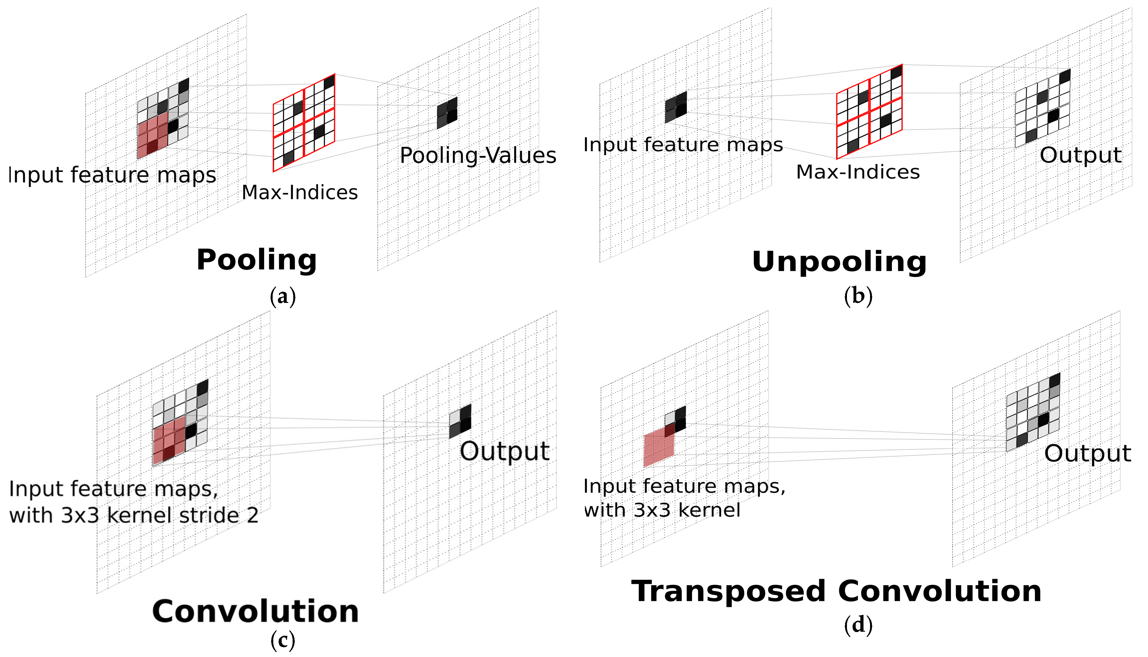
Unlike the FCN, SegNet includes the unpooling operation [30], i.e., an upsampling technique to obtain an appropriate segmentation map in a resolution identical to the corresponding original image. Instead of directly generating pixel-wise predictions from the smallest feature maps, SegNet applies the unpooling method as a step encoder in order to regenerate larger feature maps from the resulting max indices obtained from a max pooling operation in the corresponding unpooling layer, see Figure 1a,b. Following this approach, the feature indices that have the maximum value will be preserved as dominant in the upsampling procedure, often resulting in improved classification performance. In addition to the unpooling technique, deconvolutional networks or deconvnet [31] propose a “transposed” convolution operation referred to as “deconvolution”, see Figure 1d.
Another architecture of interest to our problem is the pyramid scene parsing network (PSPNet) [32]. These architectures include a pyramid pooling module that instead of using a fixed kernel size, uses kernels of different sizes to generate pyramidal convolutional layers generating multi-size feature maps. The purpose of this approach is to help improve the classification performance by more effectively incorporating a broader spatial context for the different feature map resolutions.
For our field of application, we finally consider atrous convolution architecture [23] to be of particular interest. An important advantage of this architecture is the moderate amount of pooling layers, which prevents the extensive use of rescaling procedures. Using this approach, we can avoid extensive upsampling [34].
2.2. The Atrous Convolution Architecture
In the present study, we implemented an atrous convolution architecture that resembles the deep residual network (ResNet) [19]. The main idea of the ResNet is to pass the input feature maps of a learning block, as a form of identity reference, to the final output of its block. It is hypothesized that it is easier to optimize feature maps with residual references than unreferenced ones. According to the original ideas of the ResNet, the residual learning of a particular layer is defined as:
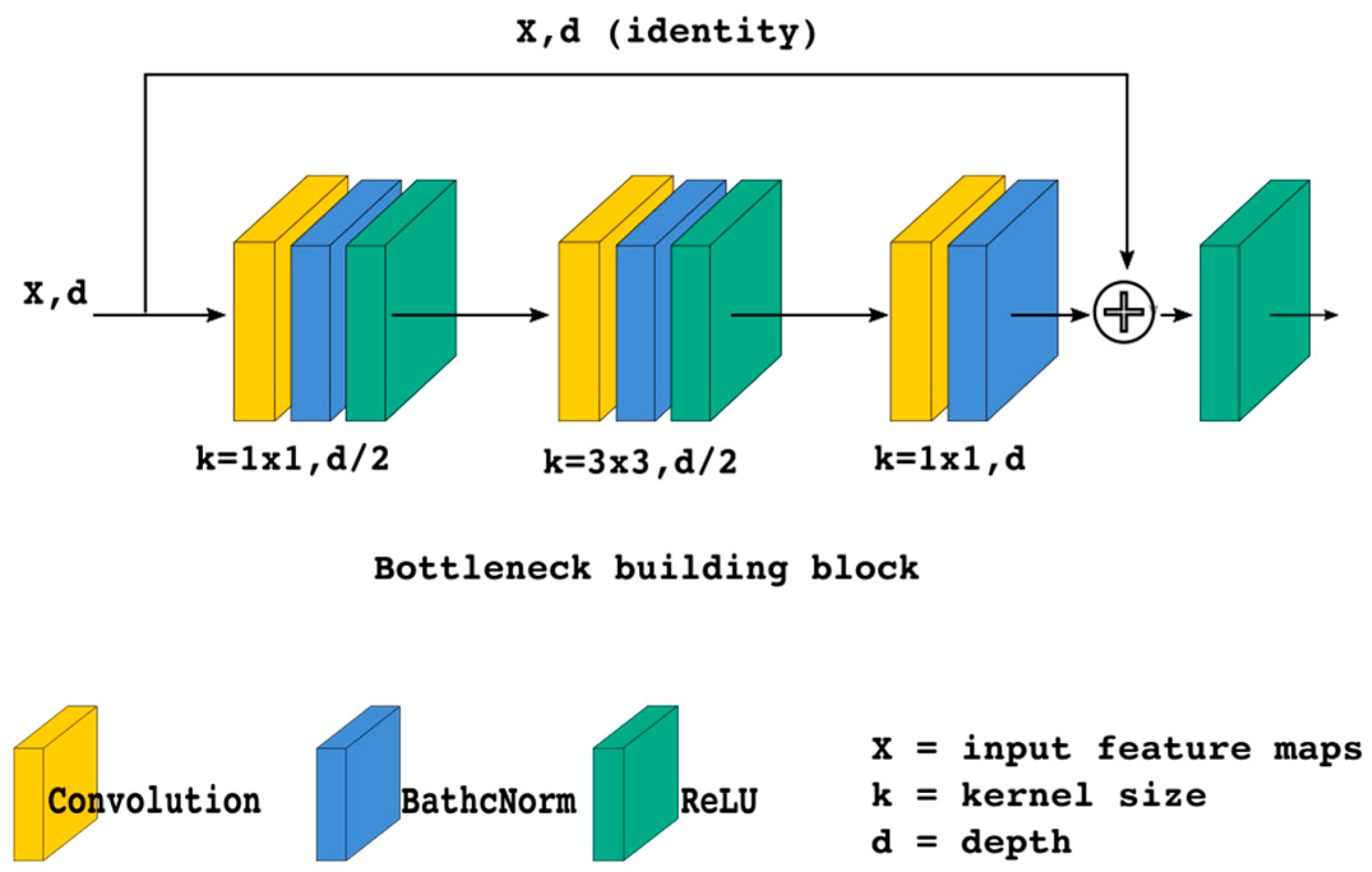
where x and y denote the representation of the input and output features of the layer, respectively. x also denotes an identity mapping from the previous block, while the function denotes the process of convolving Wi through x, including the use of rectified linear unit (ReLU) activation functions [35]. We used a residual learning called “bottleneck” building block in our research, as shown in Figure 2.
The particular variant of ResNet that we utilize here is called ResNet 101. This architecture consists of 101 residual layers with four main blocks. In the remaining parts of this paper, we will refer to each such block as a MainBlock. Each MainBlock has three, 4, 23, and three inner blocks, respectively. MainBlock 1 and 2 use 64 and 512 depth kernels, while MainBlock 3 and 4 use 1024 and 2048 depth kernels, respectively. In the atrous network, MainBlock 1 and 2 consist of several bottleneck building block using convolution kernels, while MainBlock 3 and 4 use the building blocks with atrous kernels.
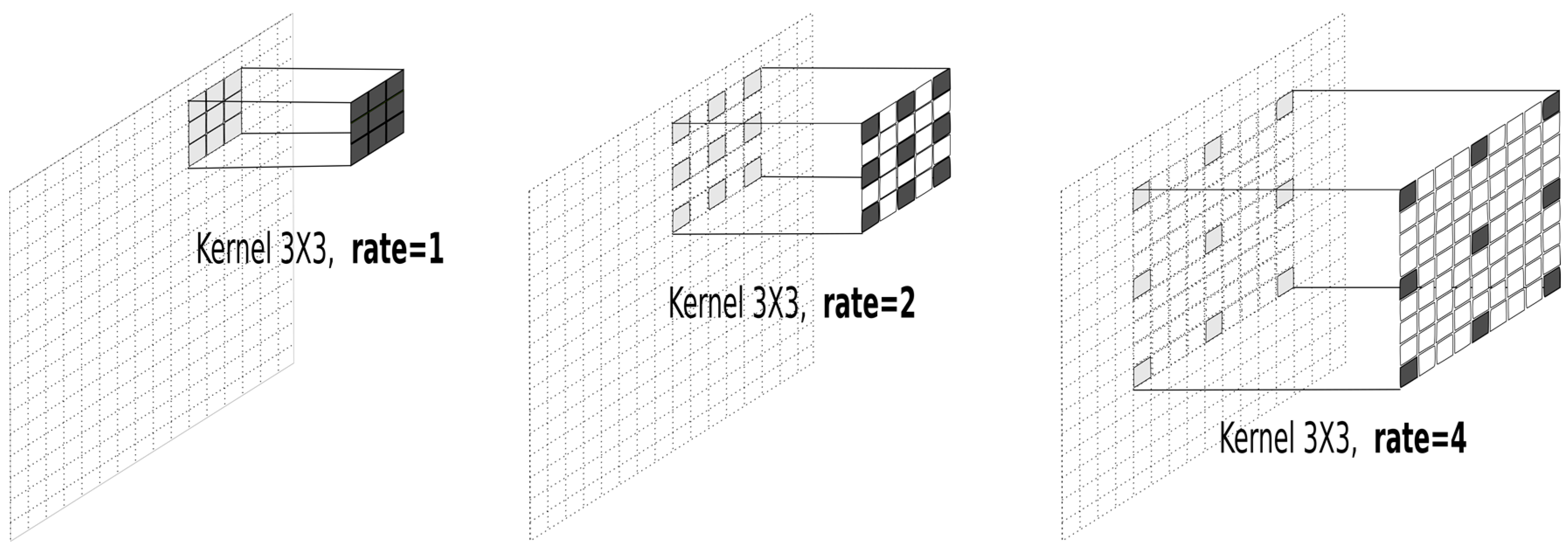
Unlike normal convolutional layers, atrous convolutions convolve through the feature spaces using a sparse kernel including gaps that are referred to as the rate, as shown in Figure 3. An atrous kernel with rate one is identical to an ordinary convolution kernel. The idea of kernels with gaps is to obtain convolutions of various aggregated regions without changing the spatial resolution of the output layer. This property enables an atrous layer to combine features that are close, but are not directly spatially connected, while maintaining the spatial resolution and avoiding the use of larger kernels. This approach allows the analysis to benefit from the presence of spatial autocorrelation in the data.
2.3. Evaluation Metrics
Various evaluation metrics can be used to determine the effectiveness of a machine learning model for predicting the unseen data. One of the most common metrics used for pixel classification problems is the pixel accuracy (PA). The PA has been frequently used in many classification tasks [25,27,36]. However, in the segmentation problem, the accuracies are commonly measured using mean pixel accuracies (MPA), mean intersection-over-union (MIoU), and the F-Measure (F1 Score). It should be noted that for segmentation problems where the total area of the classes is very different (imbalanced), the PA measure is less informative. This is because assigning all of the pixels to the largest class may result in a large PA value, even without training a model.
With k + 1 being the total number of classes (including the background class) and pij denoting the number of pixels from class i assigned to class j, the accuracy measures PA, MPA, and MIoU are defined [37] as follows:
The definition of MIoU (Equation (4)) shows that this metric considers both the valid prediction (pii) and a penalization with respect to the false negatives (pij) and false positives (pji). Training an architecture based on the MIoU contributes to making the resulting model both robust in terms of good predictions and more sensitive against the bad ones.
In addition to the MIoU, we also use the F-Measure to better evaluate the boundary region of the predicted pixels [30]. We use the mean of the F-Measure per class to evaluate the performance of the classifiers. This metric considers both the precision (p) and recall (r) of the prediction results. With TP denoting the true positives, FP denoting the false positives, and FN denoting the false negatives, the F-Measure (F1 Score) is defined as:
For the sake of simplicity, we will refer to the pixel accuracy measure as PA, the mean pixel accuracy as MPA, the mean intersection-over-union as MIoU, and the F-Measure as F1 throughout this paper.
3. Data Sources
In this section, we describe the datasets and preprocessing techniques used in our experiments prior to the deep learning training process.
3.1. Study Area and Datasets
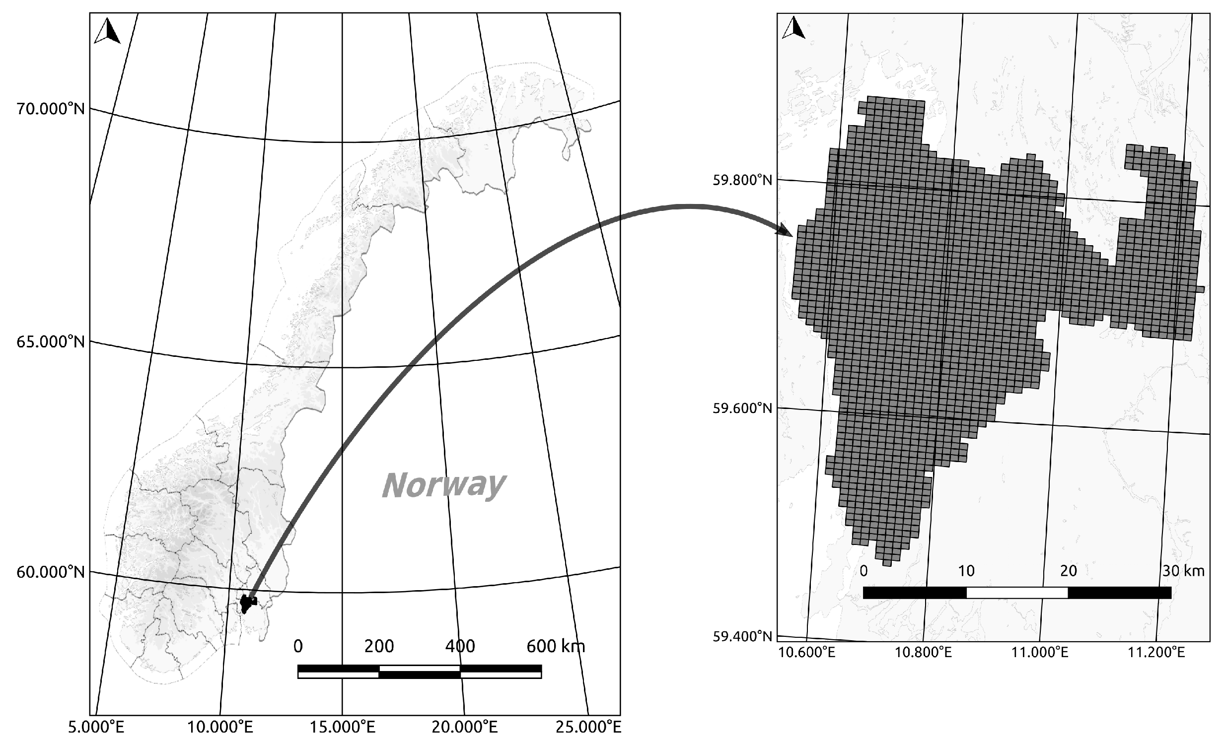
Our study area covers the Follo region, which is a part of the county of Akershus, Norway, as shown in Figure 4. Follo is located in Southern Norway, covers 819 km2, and has a relatively long coastline. It consists of moderately hilly terrain dominated by forest, with large patches of agricultural areas and smaller areas of settlement. There are also some lakes in the area.
The datasets that we have used for our research are gridded (1 m × 1 m) LiDAR point cloud data as input data, and the AR5 land resource map from NIBIO as label/ground truth data. The LiDAR data used for this research were taken from the Follo 2014 project with project number BNO14004. The project was operated by Blom Geomatics AS with a specification of 5 points/m2 covering 850 km2 using a Riegl LMS Q-780. The scan was done from 1030 m aboveground with a pulse repetition frequency of 266,000 Hz and a scan frequency of 93 Hz [38]. The LiDAR data used for this project have both LiDAR-derived features (height, intensity, number of return, and more) and image-based (red–green–blue, or RGB) features. The total number of points is approximately eight billion, which is divided into 1877 tiles that are stored in LAZ (LAS compressed files) format. Most of the tiles have a size of 600 m × 800 m (600 × 800 pixels), and each tile consists of more than 2.4 million points.
The ground truth data that we have used for this project are the NIBIO AR5 land resource dataset [7]. The dataset covers Follo and consists of four types of classification, namely land type category (arealtype, a mixture of land use and land cover classification), forest productivity (skogbonitet), tree type (treslag), and ground conditions (grunnforhold). In this project, we utilize only the land type classification, which originally covers 11 classes. Due to the non-existence or very small coverage of some of the land type classes in the Follo area, we have simplified the classification task to the modeling and prediction of the following eight classes: settlement, road/transportation, cultivation/grass, forest, swamp, lake–river, ocean, and other land types. The other land type class is a combination of undefined objects, open interpretations, and other classes with limited representation in the area (below 0.5%).
The AR5 dataset was first established in the 1960s, and has been updated continuously since 1988 for the purpose of agriculture and forest management in Norway. The precision for the agricultural classes is recorded down to 500 m2. Other areas such as forest, swamp, and open areas smaller than 2000 m2 are not registered, but include surrounding or neighboring classes. In addition, classes such as road and settlement have their origin in auxiliary datasets that have been merged into the AR5 dataset, thus resulting in a varying level of details (LoD) and accuracy for the included classes. These conditions represent considerable challenges when using the AR5 dataset as ground truth for classifying areal types based on the high-precision LiDAR dataset, since perfect classification results based on the image data are impossible to achieve.
3.2. Challenges with the AR5 Dataset
One of the most pronounced challenges with respect to learning the AR5 classes using LiDAR data is the difference in resolution. The laser data has a submeter LoD, while the AR5 dataset has a maximum resolution of 500 m2. The difference in the original resolutions clearly contributes to making the regridded ground truth class labeling data inaccurate at the 1 m2 resolution of the gridded LiDAR dataset. In addition, differences pertaining to acquisition times (last time of update) also contribute to inaccuracies in the class labeling.
There is also a notable difference between the AR5 classes with respect to their internal homogeneity. E.g., a “forest” can be composed of different tree species producing heterogeneous structures in terms of their LiDAR footprints. Parts of the forest may consist of old stands, while other stands are recent clear-cuts. In between these extremes, every age group is represented within the “forest” class.
Therefore, the accuracy with respect to the prediction of the ground truth data is correspondingly limited by these shortcomings. For example, some settlement classes are actually combinations of roads, trees, and buildings. This makes it more challenging to train a classifier to successfully distinguish between these classes.
Another practical challenge is the imbalance in the relative frequencies of the different class labels. More than 50% of the Follo area has class labels marked as Forest, and about 20% of the area has class labels marked as cultivation. The remaining areas are unevenly distributed over the other six classes. This imbalance calls for the training process to focus more intensively toward modeling the underrepresented classes.
3.3. Preprocessing Procedures
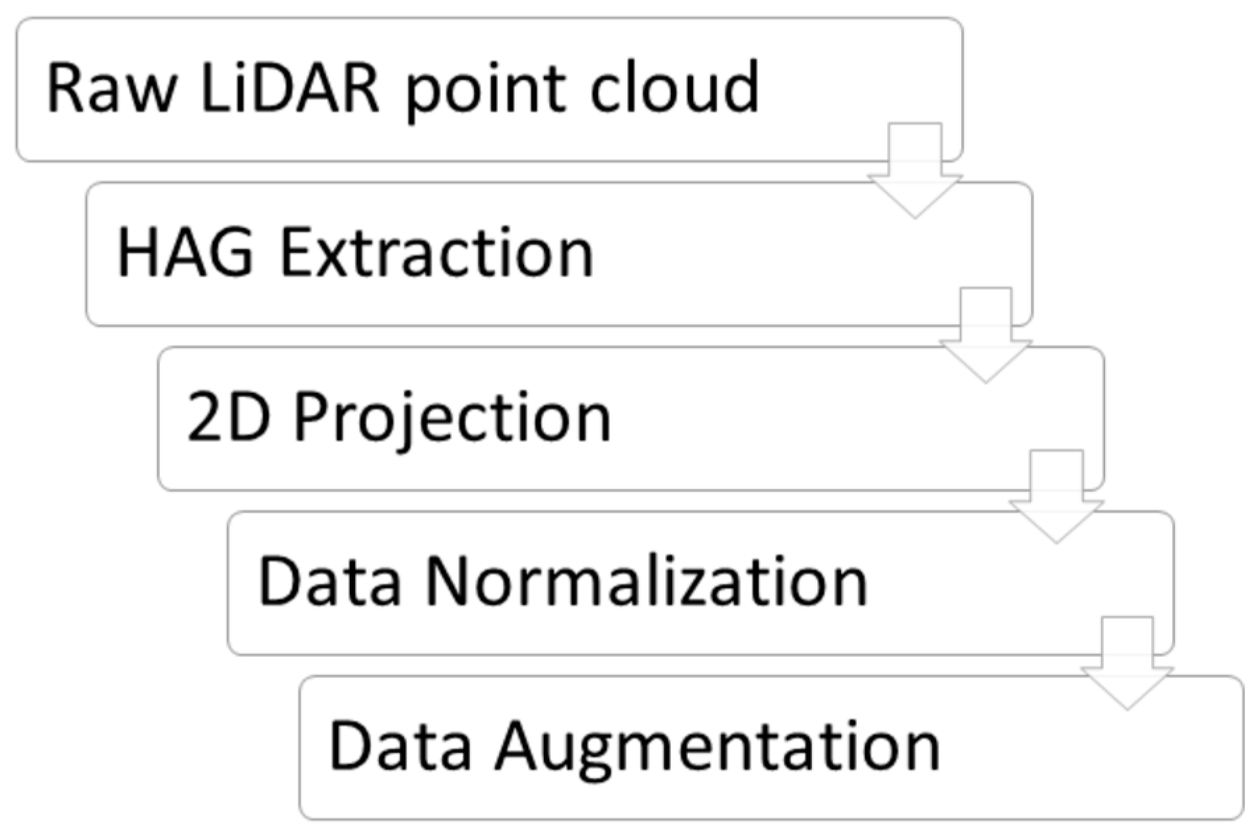
The pipeline of data preprocessing for the current investigation can be described as follows: (1) extracting of height above ground (HAG) for the LiDAR point cloud, (2) aggregating the HAG values into a two-dimensional (2D) grid, and (3) normalizing the feature values in the new representation. The summary of the preprocessing pipeline can be shown in Figure 5.
Firstly, the HAG values were extracted using a HAG filter in the point data abstraction library (PDAL) toolkit [39]. The purpose of this process was to obtain a height representation that reflects the variation in the vegetation cover and the built environment.
Secondly, in the gridding step, the LiDAR data were aggregated to a 1 m × 1 m resolution grid based on their spatial location. The AR5 dataset was therefore regridded into the same 1 m × 1 m resolution as the LiDAR data, and each cell was given a (RGB) color roughly according to the style used for the NIBIO AR5 web map service (WMS) [40]. This process was the most time-consuming step, because billions of LiDAR points required individual processing before the grid cell aggregation. The processing was completed by an extensive multi-threaded application of the LibLAS library for python.
The grid size of 1 m was chosen to be consistent with the unit size of the coordinate system that covers the laser data. Consequently, an individual point was assigned to a grid cell by truncation of its coordinate values. Aggregated values for each grid cell were from the assigned points. The most frequent value in each of the RGB channels were taken as the RGB channel values of the grid cell, while for HAG and intensity, mean values were used. Using the mean value for a high-resolution grid with (on average) five points yields small corresponding standard deviations, in particular within areas that are roughly homogenous. The complete aggregation process results in a dataset containing gridded LiDAR with RGB, HAG, and intensity as features. It should be noted that we have padded the empty grid cells with zeros, similar to zero padding in CNN [19]. This requires less computation than using an interpolation algorithm, and arguably, for a deep learning architecture, it has a similar effect on a high-density point cloud (5 points/m2) [17].
Lastly, after completing the gridding process, we performed zero mean and unit variance normalization. The values of each channel were obtained by subtracting the channel mean and dividing by the channel standard deviation. Finally, we split the normalized tiles into sets of training (70%), validation (10%), and test data (20%), respectively.
For the training data, we performed a patching process with a sliding window for each tile. We used a patch size of 224 × 224 pixels and a 168-pixel (3/4) step size. For all of the boundary patches that were smaller than the patch size, we shifted the origin of the boundary patches back and/or up so that the patches all have the size of 224 × 224 pixels. The reason for choosing a patch size of 224 × 224 is that this is the most commonly applied crop size for both the VGGnet and the ResNet architecture [19]. This choice simplifies the benchmarking process, because the other deep learning architectures that we have explored in our study were designed for the 224 × 224 patch size.
The resulting preprocessed dataset is a set of overlapping patches, where the pairwise overlap of horizontally and vertically neighboring patches is 1/4 (25%). The overlap contributes to reducing the impact of disturbing boundary effects in the resulting classifiers.
The successful training of a deep learning architecture requires access to a large number of training samples. Therefore, the final part of the preprocessing procedure is the data augmentation step. With image data, the data augmentation process is completed by generating additional data through flipping and rotating the original images. For each of the patches described above, we did a 90° clockwise rotation and up–down and left–right flipping. This process increases the dataset by 300%, and at the end of the preprocessing pipeline, we obtained a total of 57,036 patches that were available for the training process.
It should be noted that for the validation and test data, we omitted the sliding window and data augmentation parts. Most of the architectures can process images of any size; therefore, the validation and test accuracies were calculated by using the original LiDAR gridding (600 × 800 pixels) to simplify the inference process. We used the validation data for selecting the “best model” for each architecture, and the test data to calculate the final accuracies of the selected models.
The implementations for all of our experiments were based on the TensorFlow library [41] for deep learning developed by Google. The deep learning architectures were trained for at least 50 epochs with an ongoing updating of the classification accuracies on a desktop computer using 11GB GeForce GTX 1080 Ti graphics cards. The full setup for our training process of the various architectures took several weeks. However, the final and best model was trained to the reported performance in only two days.
4. The Research Process (Modeling Workflow)
The workflow of our research process was as follows. First, we carried out a number of experiments by training several well-known deep learning architectures for semantic segmentation with our data. The purpose of these experiments was to identify the baseline level of classification performance, and generate the required experiences to propose some of the potentially useful alternative architectures for later benchmarking. It should be noted that the initial experiments only included image-based (RGB) features, since architectures designed for using LiDAR data are hardly available.
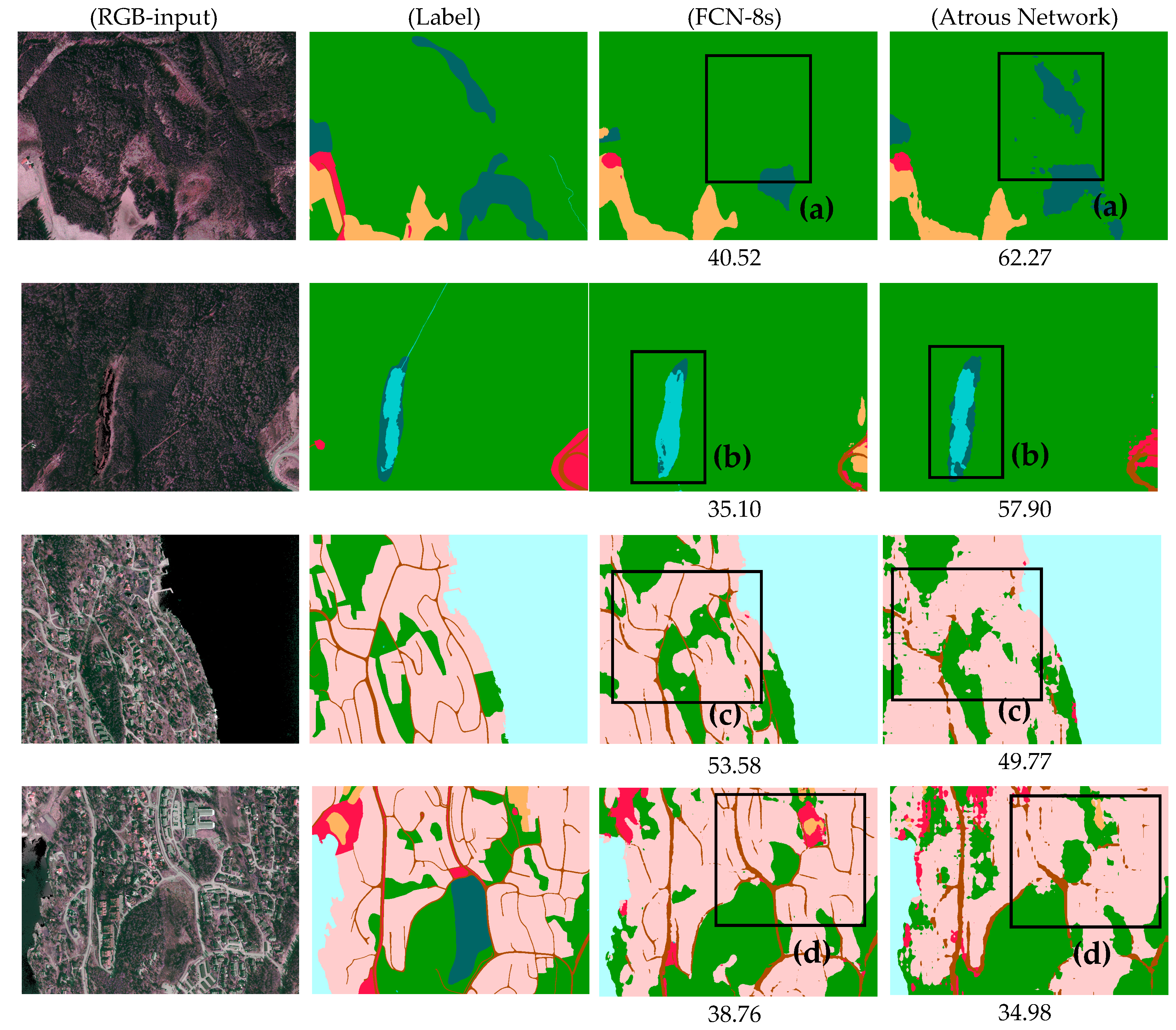
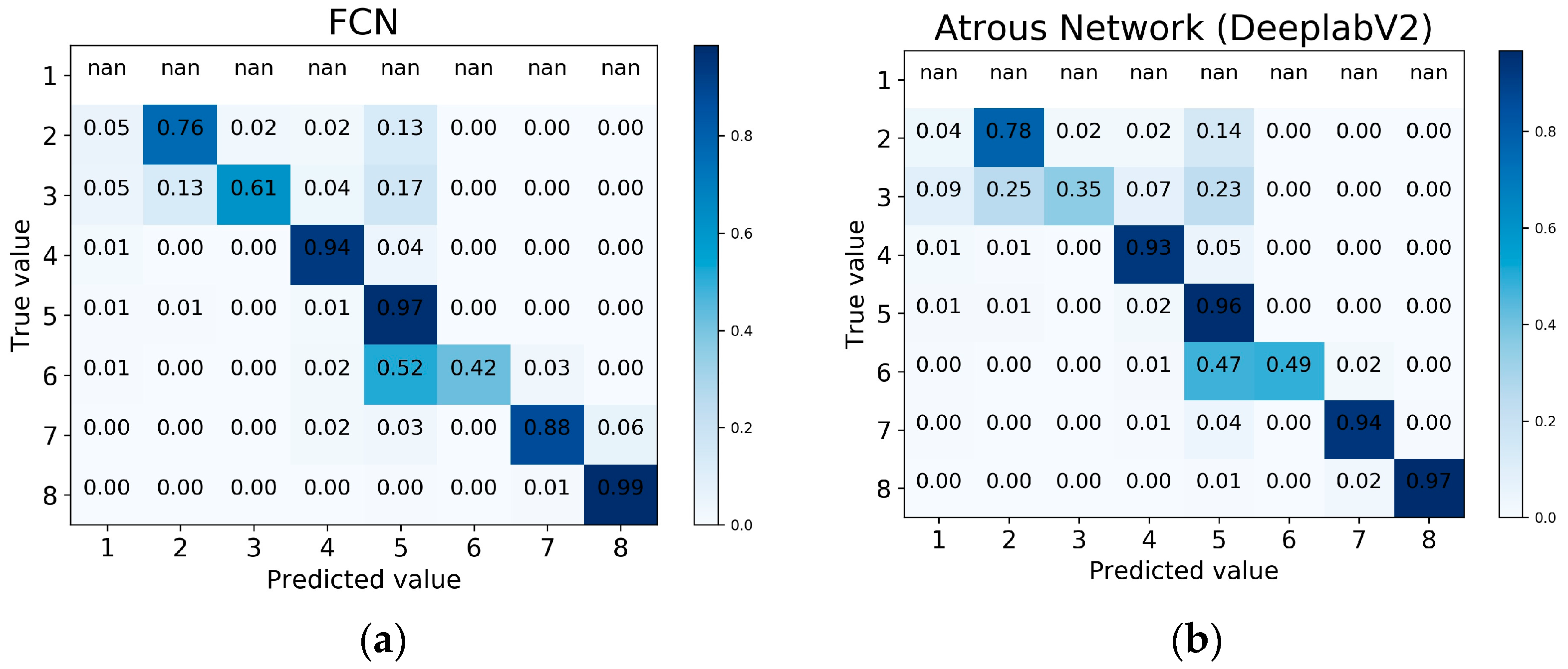
Based on the experimental results, we did an elementary qualitative analysis by inspecting the predicted output masks (Figure 6) and associated confusion matrices (Figure 7). Among our notable findings were that the classifier obtained by training an atrous network generalized considerably better than the classifier obtained by the FCN-8s architecture. In Figure 6a, the FCN-8s erroneously predicted most of the area to be green. In Figure 6b, we see that the FCN-8s generalizes too heavily for the highlighted area. We argue that this is most likely due to the effect of the small receptive field in the FCN kernel. The atrous network, on the other hand, was quite successful in predicting the most common classes, but it failed more frequently in predicting the less common ones.
We also noted that the atrous network upsampling, which utilizes a nearest neighbor technique, failed to generate a valid prediction mask. Figure 6c,d shows the insufficiency of this upsampling technique in recovering the thin and linear class of roads. We suspect that this insufficiency is closely related to the upscaling technique being part of the atrous network’s architecture.
With the ambition of preserving the advantages of the above architectures, and compensating for their limitations, we were lead to propose an alternative architecture for our classification problem. The proposed alternative architecture included atrous convolution kernels for improved generalization and the FCN-based upsampling approach to strive for predictions that are less coarse. In addition, we incorporated the softmax with IoU loss function, which is known to be effective in other architectures. We also included LiDAR-derived features such as HAG and intensity together with an effective merging technique to include the additional features, aiming at improving the classification performance of our alternative deep learning proposals.
4.1. Baseline Experiments
An initial investigation based on modeling exclusively with RGB features is required to establish the benchmark classification performances associated with various existing deep learning architectures for our problem. We started out this investigation by exploring four different architectures, i.e., the DeconvNet, the SegNet, the FCN-8s, and the atrous network from DeepLab.
The first architecture that we explored was the DeconvNet, where we used Fabian’s implementation [42] with five full convolutional blocks followed by five deconvolutional blocks. The architecture was trained using a mini batch gradient descent strategy by including 15 images per iteration. The training process was based on the Adam optimizer [43] with an initial learning rate of 1 × e−4. By training from scratch (no utilization of a pre-trained model for this architecture), two weeks of training was insufficient for obtaining a satisfactory classification model. We therefore decided to abort the training process at that stage, and not pursue the training of this architecture any further.
The second architecture that we explored was the SegNet, where we used the Aerial Images implementation from Ørstavik [44] (called AirNet). We implemented the AirNet using five encoders and five decoders in a SegNet architecture with training based on the AdaGrad [45], including a dropout technique acting as regularization [46] to prevent against overfitting. The dropout works by ignoring a certain percentage of its neurons randomly in each epoch of the training process.
The initial learning rate for AirNet was set to 1 × e−4, and the architecture was trained from scratch for 90 epochs (with an additional 40 epochs due to not utilizing a pre-trained model). The resulting model obtained an accuracy of 59.12% in terms of MIoU and 92.11% in terms of PA. It should be noted that the test accuracies for AirNet were calculated using test data with a sliding window of 224 × 224 and no augmentation. This is due to the limitation of the unpooling module of this architecture to address dimensions of 600 × 800, which were the dimensions on the original test data.
The third architecture that we explored was the FCN-8s architecture. We used the FCN-8s implementation from Shekkizhar [47]. Shekkizhar’s FCN-8s was built based on VGGnet architecture. We trained the model by using the Adam optimizer and fine-tuned it by using VGGnet weights obtained from MatConvNet [48]. Similar to the SegNet, the FCN-8s was also trained with regularization by using the dropout technique. The initial learning rate was set to 1 × e−4, and the architecture was trained for 50 epochs. Interestingly, by using the straightforward upsampling technique of FCN-8s, a MIoU equal to 64.97% was obtained for the test data.
The last architecture that we explored was the deeplabV2 [23], which utilized an atrous convolution layer on top of a ResNet architecture; we called it the atrous network. For training this architecture, we utilized the DeepLab–ResNet architecture rebuilt in TensorFlow, as seen in Vladimir’s implementation [49]. The atrous network implementation was trained with an initial learning rate of 2.5 × e−4 and a weight decay of 0.0005. The training process was optimized using a momentum update [50] with a momentum value of 0.9 and batch normalization [51] to reduce the internal covariate shift due to the parameters update during back propagation. The nearest neighbor technique was used to upsample the final feature maps back into the original input size, before calculating the accuracies.
Two approaches were used to calculate the test set prediction accuracies for the atrous network architecture. The first one included the post-processing conditional random field (CRF) [52], and the second one did not. It should be noted that by skipping the CRF post-processing, we obtained the better classifier, as seen in Table 1.
4.2. The FCN-Based Architectures Including IoU Loss
The results obtained by using the atrous network revealed to us some weaknesses due to the application of a non-learnable upsampling technique, as seen in Figure 6. We therefore decided to integrate the FCN upsampling technique with the atrous network’s architecture in order to try to overcome these problems.
In order to integrate the ResNet–FCN [53] and the atrous kernel, we modified the third and fourth MainBlock of the ResNet-FCN with atrous kernels with rates of two and four, respectively. The output of the last three MainBlocks were upsampled using transposed convolution to get the same size of the output as for the first MainBlock, and all of the MainBlock outputs were combined by using the addition operator. Note that before combining, the first MainBlock was updated with an additional convolution layer using a 1 × 1 kernel with a depth of eight and a stride of one. Finally, the original image size was recovered using a transposed convolution, as shown in Figure 8.
The main idea summarized in the resulting architecture reflects the desire to obtain a model that is capable of looking widely for the appropriate feature maps by using the atrous kernels. Simultaneously, the ability of learning the upsampled feature maps is maintained by using transposed convolutions. We will refer to this architecture as the Atrous-FCN.
We explored the possibilities of training with both the softmax with cross-entropy loss function [54], and the softmax with IoU loss function [26]. The results were compared in a quantitative analysis. The reason for exploring the IoU type of loss function is to try to make the network more robust against bad predictions, as the IoU metric penalizes against both false positives and false negatives. With TP denoting the true positives, FP denoting the false positives, and FN denoting the false negatives, the original IoU is defined as:
By using a loss function closely related to the MIoU metric, we experienced that the training was effective not only for speeding up the training process, but also for improving the classification performance.
The IoU (Equation (8)) is by definition a non-differential function that cannot be used directly with the back-propagation algorithm. Fortunately, Rahman et al. has proposed an approximation of the IoU by a differentiable function that replaces the counting operations with multiplications and additions [26]. For a binary classification problem, they proposed a formulation of the IoU by considering the ratio between intersection I(X) and union U(X), where I(X), U(X), and the IoU loss () were defined as:
Here, V is the set of all of the pixels in the image, X is the pixel probabilities obtained by a sigmoid function, and are the ground-truth values. Y = 0 represents the background pixel label, and Y = 1 represents the object pixel label in this notation.
The implementation of the IoU loss in our application had to be done slightly differently, because our classification problem was non-binary. In our solution, we used a softmax approach to obtain the pixel probabilities for each class. Subsequently, we used the one-hot encoding to enable the binary classifiers to handle the multiclass ground-truth data. The (Equation (11)) was used to calculate the losses for each class, as well as a summation of all of the losses, which was used to reflect the final loss of the network. Note that the weight-regularization loss approach [55] was not included in our implementation.
For a final comparison, the ResNet-FCN with cross-entropy loss, the ResNet-FCN with IoU loss, and the Atrous-FCN with IoU loss were all fine-tuned using the pre-trained model from DeepLab-ResNet [49]. Each network was trained for 50 epochs using a momentum update with the same initial learning rate of 0.01. The test results are shown in Table 2.
The results in Table 2 demonstrate the effectiveness of the IoU loss function. By only changing the loss function on a ResNet-FCN, the test accuracies improved with 3.19% on MPA and 2.67% on MIoU. In addition, the test result also confirmed the advantage of integrating the ResNet-FCN with atrous kernel. The Atrous-FCN reached the MIoU of 66.52%, which was a 3.71% improvement from the original atrous network (Table 1).
It should be noted that implementing atrous kernels on top of ResNet-FCN requires substantially more memory, which slows down the training process. This is because the atrous kernels maintain the larger feature maps of the deeper layers (output stride of eight). Therefore, convoluting through the larger feature maps and deeper architectures requires a significant amount of memory for holding the larger number of parameters. When using an 11GB GeForce GTX 1080 Ti, the Atrous-FCN required 43 min to process a single training epoch.
4.3. The Stochastic Depth Extension
In order to speed up the Atrous-FCN, we therefore decided to integrate it with the stochastic depth paradigm. The resulting architecture is referred to as the Stochastic Atrous Network (SA-Net).
The stochastic depth paradigm comes with the idea of wanting much shorter training times. It is implemented by randomly skipping some layers in each epoch of the learning process [24]. Inclusion of the stochastic depth approach has been demonstrated both to speed up the learning process and cause an advantageous regularization effect for the training process.
In the original publication [24], stochastic depth in a residual building block of a ResNet is defined as:
where bl denotes a Bernoulli random variable with values 0 or 1, and represents the active (bl = 1) or inactive (bl = 0) of the lth residual learning block, while the rest is a residual block with the ReLU activation function, which has been explained in Equation 1. bl is controlled by another set of hyperparameters called survival probabilities and marked as pl. This value decides the randomness degree of bl. Stochastic depth networks commonly implement the linear decay of the value of its survival probabilities (pl): the deeper the layer, the smaller its probability for survival.
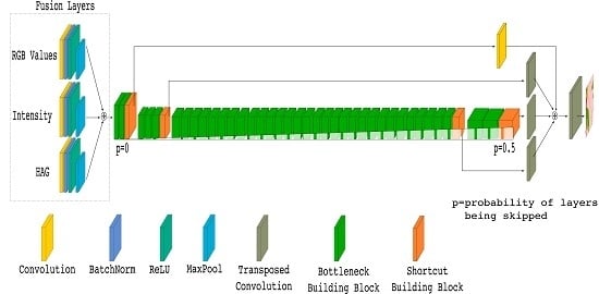
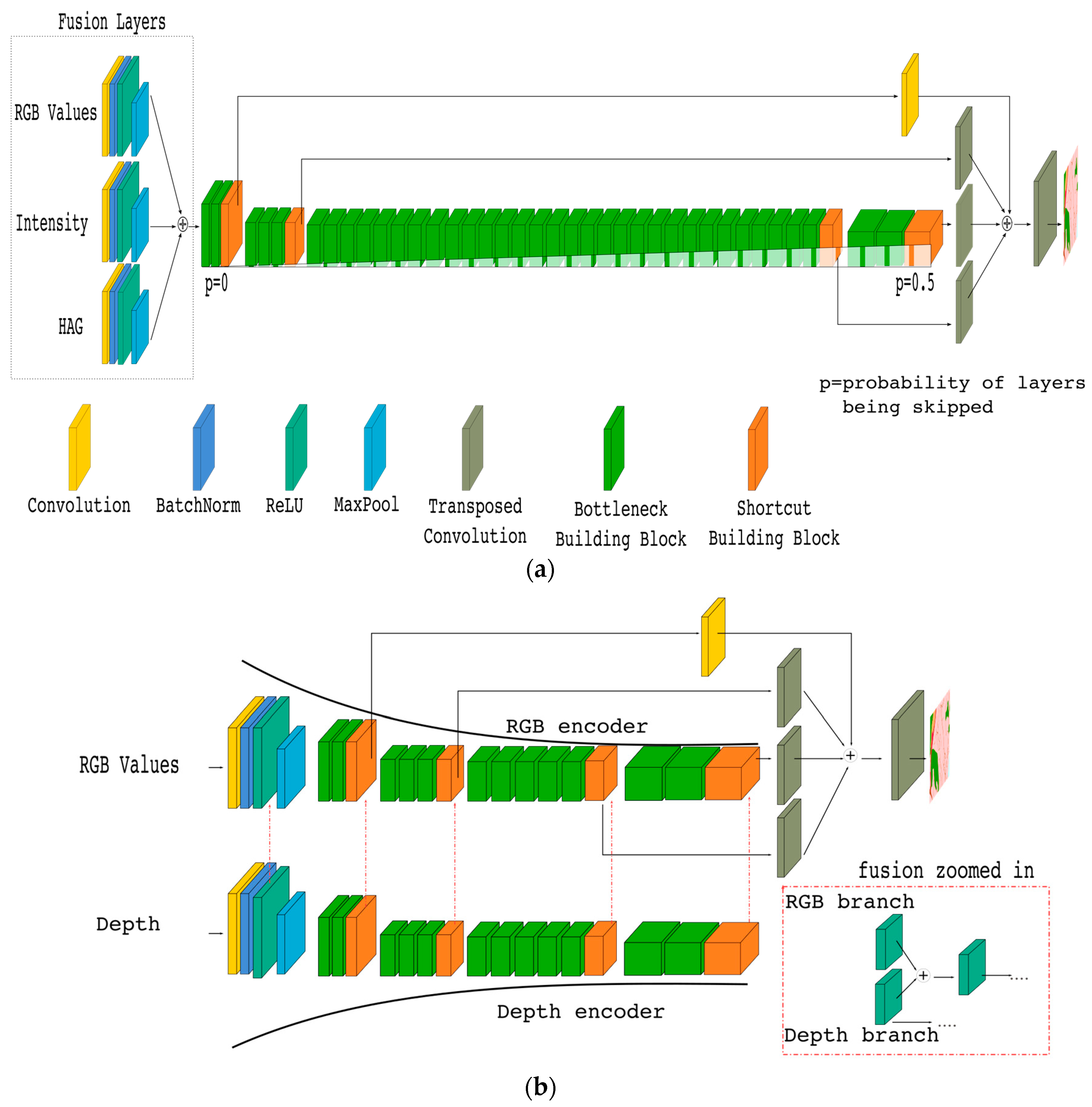
The integration of the stochastic depth approach with our atrous-FCN architecture is a straightforward procedure, because it is already developed for use with a ResNet architecture. The final structure of the suggested SA-Net architecture is shown in Figure 9a (at the present stage, ignore the fusion layers, except for the RGB input).
We attached the stochastic depth mechanism to all of the bottleneck building blocks on Atrous-FCN by using an 0.5 linear decay. This means that the probability of a block being skipped is increased linearly up to 50% at the end of the final building block. Our training and test results show that by including the stochastic paradigm, the training time was reduced by 30%, while the test set MIoU values increased slightly to 66.67%, as seen in Table 2.
4.4. The Final Extension Including More Features by Data Fusion
The purpose of data fusion in deep learning is to improve the resulting classifiers by merging more types of data (such as intensity and HAG from the LiDAR measurements) with the traditional RGB image data to get an even better representation of the problem domain. However, such merging is not always successful, and we have experienced that extending a deep learning architecture to incorporate non-RGB channels does not always lead to improved classification performance (the introduction of noisy data can sometimes corrupt the training process and damage the final classification performance).
An extension of the proposed SA-Net approach to include data fusion provides the final architecture of our investigation. The required extension from SA-Net is quite straightforward, as shown in Figure 9a. We refer to this architecture as the EarlyFusion SA-Net. The idea of data fusion in deep learning relates to the FuseNet architecture [56].
The original FuseNet architecture was built with the 16-layer VGGnet [33] using an encoder–decoder, SegNet-style architecture. The FuseNet uses two branches of encoders: one RGB encoder and one depth encoder. The output of each of the Convolution + Batch Normalization + ReLU (CBR) layers of the depth encoder is combined with the output of the corresponding CBR layers of the RGB-encoder using addition. The convolution block in a CBR consists of 64 convolution layers with 7 × 7 kernels and a stride of two, followed by Batch Normalization [51] and the ReLU activation function.
Our implementation of the FuseNet is based on our SA-Net architecture (Figure 9b), where we include two branches of encoders, which were both created by using the stochastic atrous approach with different kernels. In the fusion process, we combine the output from each MainBlock of the depth-encoder branch with the RGB MainBlock output using the same fusion technique as in the original FuseNet. The decoder part was built using the FCN upsampling approach with transposed convolutions and skip connections.
The models obtained by training our implementation of the FuseNet style architecture turned out to perform below our expectations. With a big network and huge memory footprint, the best test set accuracy that we achieved was only 65.49% for MIoU and 93.38% for PA. One of the main challenges seemed to be that the separated branches of depth and RGB encoders consumed most of the graphics processing unit (GPU) memory. Due to this, the GPU was only capable of training 50 layers, compared with the 101 layers in the SA-Net architecture.
The experiences from the FuseNet style approach actually helped us in specifying the EarlyFusion SA-Net architecture (Figure 9a). Instead of creating separated encoders for different types of input data, we realized that using only one encoder might be advantageous. The solution was to assemble three CBR blocks for individually processing the RGB, Intensity, and HAG data. Each CBR block was equipped with its own kernel, and the outputs from the blocks were combined by addition into the fusion layers. Before taking the combinations, pooling layers using 3 × 3 kernels with a stride of two were included at the end of each CBR block (to reduce the feature maps to have an output stride of four). The resulting fused inputs where then integrated with the SA-Net architecture, as shown in Figure 9a. Based on this approach, we managed to reduce the number of required blocks in the encoders, allowing the incorporation of additional types of input data.
Our EarlyFusion SA-Net approach was trained using a combination of RGB, Intensity, and HAG features (all normalized by using zero mean and unit variance). All of the networks were trained with the IoU loss function and an incorporation of momentum update for optimization [50] with an initial learning rate of 0.001.
The models were fine-tuned with a modified pre-trained model inspired by the pre-trained FuseNet model described in C. Hazirbas et al.’s work [56]. The non-RGB kernels were initialized by using the mean value of the pre-trained RGB kernel (the values for the channels in the RGB kernel were summarized and divided by three, as the RGB has three input channels). This initialization strategy was applied for both the HAG and the Intensity convolution kernel. Each model was trained for 50 epochs, and the results are shown in Table 3.
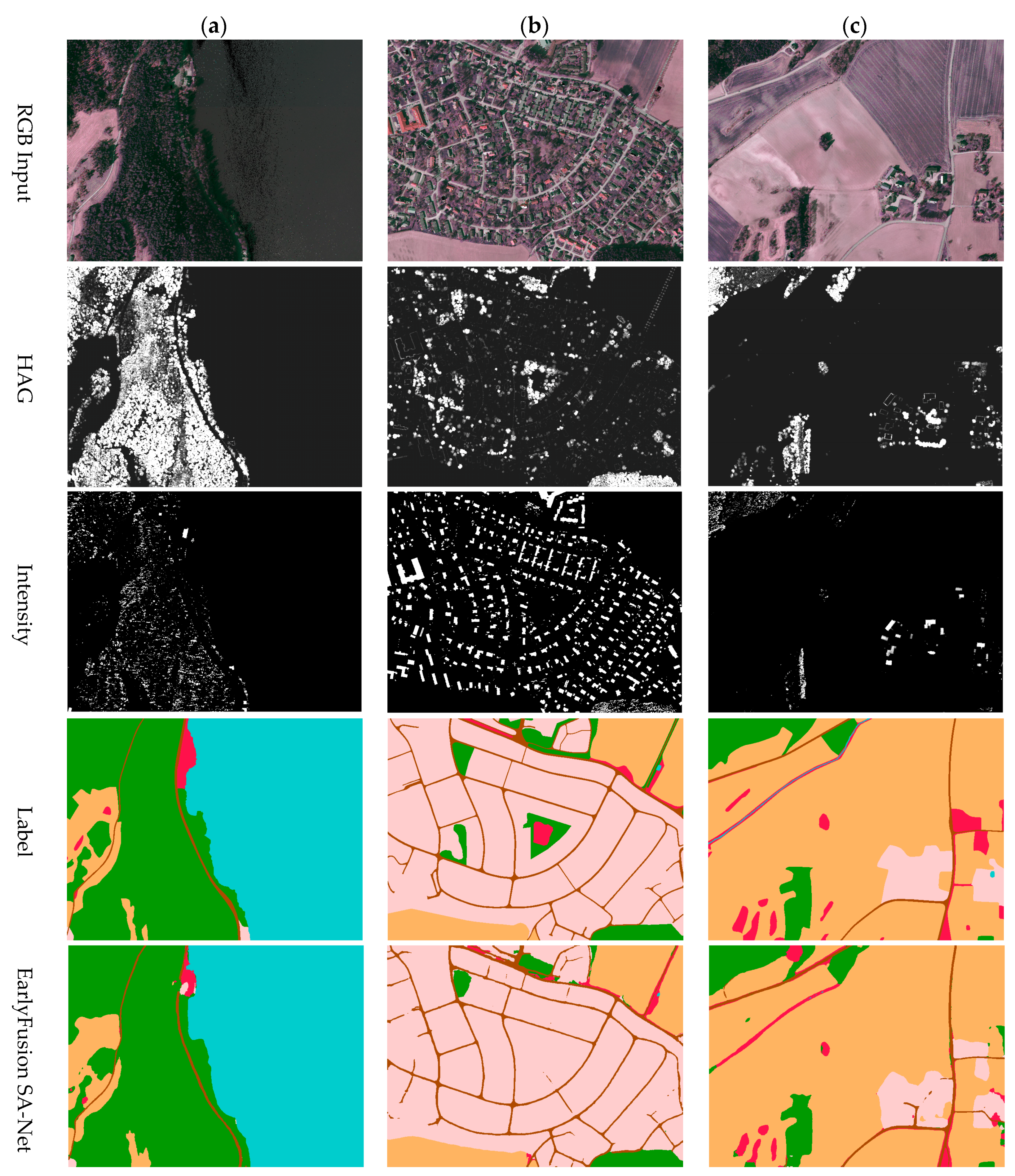
Using the same types of input (RGB and HAG), our EarlyFusion approach and the Fusenet style architecture obtained MIoU values of 67.40% and 65.49%, respectively. Incorporating intensity, our model achieved the highest MIoU values of 68.51%, which is a 5.7% relative improvement from the original atrous network (Table 1). The qualitative results of our EarlyFusion SA-Net is shown in Figure 10.
5. Discussion
5.1. Interesting Insights
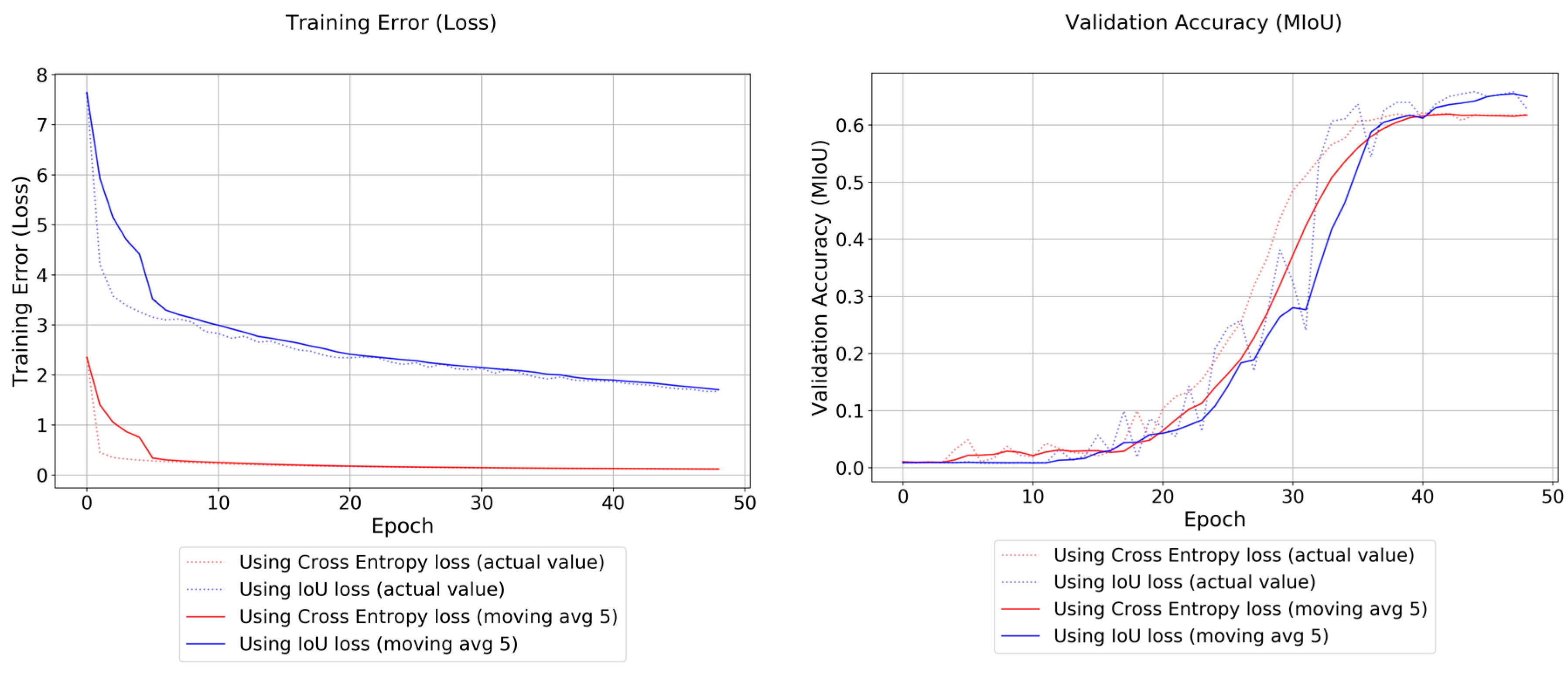
We consider the most interesting finding of the present research project to be the significant contribution of the IoU loss function in increasing accuracies. By changing the loss function from cross-entropy loss to IoU loss, the test accuracies increased by more than 3%. It should be noted that the training error (loss values) of the IoU loss decreased steeper than for cross-entropy, as seen in Figure 11. We assume that this is not just due to the different scaling of loss values, but also due to a reflection of a better error representation.
Looking through the behavior of the IoU loss in Figure 11, the accuracy of the ResNet-FCN could most likely be improved by additional training time. With 50 epochs of training time, the loss values were still decreasing steadily, and the accuracies were increasing steeply even in the last training iterations. It should be noted that we stopped at 50 epochs to make the training iterations comparable with the number of training epochs executed for the other methods.
Another interesting finding was concerned with the stochastic depth paradigm. In our experience, the SA-Net with the stochastic depth approach protects against overfitting considerably better than the Atrous-FCN. Figure 12 shows the seemingly superiority of the Atrous FCN training accuracy (MIoU) over SA-Net, which is due to considerable overfitting. This was confirmed by the validation accuracies. The highest peak on the training accuracies (MIoU) for Atrous-FCN and SA-Net were 77.25% and 73.16%, respectively, and the validation accuracies for MIoU were 66.52% and 66.67%, respectively.
SA-Net’s ability to resist overfitting opens an opportunity in simplifying the training process. For limited training data, one can rely on the stochastic depth strategy to prevent overfitting and train the model with all of the data, including the validation data. With additional regularizations, such as weight regularization and dropout, this approach could contribute to even better predictions in terms of test set accuracies.
Another of our findings was related to the use of HAG and Intensity features to improve the prediction accuracies. The test set results in Table 3 shows a negative effect from combining RGB with Intensity only, reducing the test set MIoU values from 66.67% to 62.39%. LiDAR intensity is mainly determined by the reflectance characteristic of the reflector object, which shows the strength of the reflection of light [57]. This is similar to the optical sensors that produce RGB image data. This similarity amplifies the information contained in the RGB data, and also amplifies the noise in the data, resulting in a poor classifier.
In contrast, combining HAG with RGB improved the classification accuracies. HAG contains elevation information. This type of information is not captured in the image data, and our Earlyfusion architecture successfully manages to combine this into an improved classifier.
LiDAR data contain not only HAG and intensity features, but also Z-values, number of returns, flight angle, flight direction, and point classification. It is also possible to generate simple handcrafted features such as sparsity, planarity, linearity, and many more [13]. Incorporating those features with our fusion approach could potentially improve the performance of a resulting classifier.
5.2. Ground Truth Refinement
The different resolution/LoD of the LiDAR and the NIBIO AR5 data makes it difficult to obtain a good quantitative performance for the final model. Actually, we cannot expect (or aim for) a complete match between the classification and the ground truth. A certain mismatch will always be present due to both temporal and geometrical differences between the input data and the data used as ground truth.
The qualitative assessments of the results from our best model show that the prediction map in many locations actually may be more correct than the ground truth map, because the prediction identifies areas where the land cover or land use has changed after the last incremental maintenance of the land resource map. This could make the proposed model a potentially powerful tool for a guided incremental update of the AR5 ground truth dataset, making it possible to produce higher-resolution agricultural maps.
Inspecting the final predictions in Figure 10 and using local knowledge, it is actually fair to claim that our prediction results are better than the labeled data. The image data in Figure 10b,c show that our classifier can correctly predict some roads and forest patches that have been ignored in the label data. Figure 10a also shows that the classifier can predict the existence of small settlement and cultivation classes, even if they have been removed from the label data as a result of the cartographic generalization process.
Our model can be used during the incremental update of AR5 by taking advantage of the probability prediction maps. The probability prediction maps are the output from the final softmax layer of the architecture. They show the confidence in the classification. A reasonable hypothesis is that locations classified differently by our model and the label data are likely to represent real changes, in particular if the probability of the prediction is high. This hypothesis has to be subject to another study. If it is correct, then our method can be used to streamline the maintenance of the AR5 dataset by efficiently directing the attention of the cartographers toward the areas where changes are most likely to be found.
Taking this use of the model one step further, human inspection or a trained regression classifier could be used to refine the thresholds and provide better trained weights. This approach could simplify the refinement process and increase the potential for full automation of the maintenance of the land resource map.
6. Conclusions
In this paper, several novel architectures for predicting land cover segmentation using airborne LiDAR data is presented. The main contribution of our research is the development of a scalable technique for doing dense-pixel prediction that incorporates image-based features and LiDAR-derived features, to update a generalized land resource map in Norway. With the aim to understand the behavior of ground-truth data constructed from different sources and with varying resolution of the label classes, we managed to develop a deep learning architecture (the EarlyFusion SA-Net) that is not only capable of predicting generalized classes, but also identifying the less common ones. In the preprocessing procedures of our work, we projected the three-dimensional (3D) laser data to a two-dimensional (2D) representation, and used RGB, HAG, and Intensity as the features of interest. As for the classifier, SA-Net was introduced, which is a deep learning architecture using atrous kernels on a ResNet-FCN architecture using the stochastic depth technique. The atrous kernel is robust for feature generalization based on spatial autocorrelation, the ResNet-FCN provides a simple yet powerful learnable upsampling technique, and the stochastic depth with its layer regularization is not only helpful for speeding up the training process, it is also capable of improving the prediction performance. The IoU loss was also implemented, and was shown to increase the accuracies for our particular dataset. In addition, an Earlyfusion layer proved helpful for combining image-based features and LiDAR-derived features.
Experiments were carried out on the Follo 2014 LiDAR dataset with the NIBIO AR5 as ground-truth data. Comparisons were made with other deep learning-based architectures for segmentation, namely DeconvNet, SegNet, FCN-8s, and the atrous network (DeeplabV2). Experimental results show that our proposed architectures were better than the other architectures. Accuracy, when calculated using MPA and MIoU, increased by more than 5%.
With the increasing availability of LiDAR data and the advancement of LiDAR technology, more and more high-quality LiDAR data can be accessed with ease. That and the maturing of deep learning technology can significantly simplify the automatic generation of high-resolution land cover, land-use, and land-change maps. Our research provides a scalable and robust way of transforming LiDAR data to a more meaningful map of information. Further improvement may be achieved by additional training with a deeper atrous layer, by implementing stochastic depth and fusion, or a combination of both. Improvements could also be achieved by adding more features of interest from the LiDAR data and by skipping the validation and increasing the use of stochastic procedures with additional regularization.
Author Contributions
H.A.A. wrote the paper, processed the data, performed the experiments, and proposed the architectures. G.H.S. provided the AR5 dataset, contributed to the discussion, and revised the paper. H.T. supervised the study and revised the paper. U.G.I. oversaw the research, provided the statistical analysis, and revised the paper.
Acknowledgments
We would like to thank J. Wu for providing the code for the ResNet-FCN. We also would like to thank all the Github authors, whose code we used for experiments. Norwegian Mapping Authority and NIBIO are acknowledged for providing the LiDAR data and the AR5 dataset, respectively. We gratefully acknowledge all the anonymous reviewers as well as their constructive notes and reviews, through which the manuscript was enriched and improved.
Conflicts of Interest
The authors declare no conflict of interest.
References
- Norwegian Mapping Authority. Nasjonal Detaljert Høydemodell. Available online: https://www.kartverket.no/Prosjekter/Nasjonal-detaljert-hoydemodell/ (accessed on 4 February 2018).
- Norwegian Mapping Authority. Høydedata. Available online: https://hoydedata.no/LaserInnsyn/ (accessed on 5 February 2018).
- Jaboyedoff, M.; Oppikofer, T.; Abellán, A.; Derron, M.-H.; Loye, A.; Metzger, R.; Pedrazzini, A. Use of lidar in landslide investigations: A review. Nat. Hazards 2012, 61, 5–28. [Google Scholar] [CrossRef]
- Koetz, B.; Morsdorf, F.; Van der Linden, S.; Curt, T.; Allgöwer, B. Multi-source land cover classification for forest fire management based on imaging spectrometry and lidar data. For. Ecol. Manag. 2008, 256, 263–271. [Google Scholar] [CrossRef]
- Morsy, S.; Shaker, A.; El-Rabbany, A.; LaRocque, P.E. Airborne multispectral lidar data for land-cover classification and land/water mapping using different spectral indexes. ISPRS Ann. Photogramm. Remote Sens. Spat. Inf. Sci. 2016, 3. [Google Scholar] [CrossRef]
- L’heureux, A.; Grolinger, K.; Elyamany, H.F.; Capretz, M.A. Machine learning with big data: Challenges and approaches. IEEE Access 2017, 5, 7776–7797. [Google Scholar] [CrossRef]
- Bjørdal, I.; Bjørkelo, K. Ar5 Klassifikasjonssystem—Klassifikasjon av Arealressurser; Norsk Institutt for Skog og Landskap: Ås, Norway, 2014. [Google Scholar]
- Guo, B.; Huang, X.; Zhang, F.; Sohn, G. Classification of airborne laser scanning data using jointboost. ISPRS J. Photogramm. Remote Sens. 2015, 100, 71–83. [Google Scholar] [CrossRef]
- MacFaden, S.W.; O’Neil-Dunne, J.P.; Royar, A.R.; Lu, J.W.; Rundle, A.G. High-resolution tree canopy mapping for new york city using lidar and object-based image analysis. J. Appl. Remote Sens. 2012, 6, 063567. [Google Scholar] [CrossRef]
- Yan, W.Y.; Shaker, A.; El-Ashmawy, N. Urban land cover classification using airborne lidar data: A review. Remote Sens. Environ. 2015, 158, 295–310. [Google Scholar] [CrossRef]
- Zhou, W. An object-based approach for urban land cover classification: Integrating lidar height and intensity data. IEEE Geosci. Remote Sens. Lett. 2013, 10, 928–931. [Google Scholar] [CrossRef]
- Guo, L.; Chehata, N.; Mallet, C.; Boukir, S. Relevance of airborne lidar and multispectral image data for urban scene classification using random forests. ISPRS J. Photogramm. Remote Sens. 2011, 66, 56–66. [Google Scholar] [CrossRef]
- Grilli, E.; Menna, F.; Remondino, F. A review of point clouds segmentation and classification algorithms. Int. Arch. Photogramm. Remote Sens. Spatial Inf. Sci. 2017, 42, W3. [Google Scholar] [CrossRef]
- Poux, F.; Hallot, P.; Neuville, R.; Billen, R. Smart point cloud: Definition and remaining challenges. ISPRS Ann. Photogramm. Remote Sens. Spat. Inf. Sci. 2016, 4, 119. [Google Scholar] [CrossRef]
- Barnea, S.; Filin, S. Segmentation of terrestrial laser scanning data using geometry and image information. ISPRS J. Photogramm. Remote Sens. 2013, 76, 33–48. [Google Scholar] [CrossRef]
- Garcia-Gasulla, D.; Parés, F.; Vilalta, A.; Moreno, J.; Ayguadé, E.; Labarta, J.; Cortés, U.; Suzumura, T. On the behavior of convolutional nets for feature extraction. arXiv, 2017; arXiv:1703.01127. [Google Scholar]
- Krizhevsky, A.; Sutskever, I.; Hinton, G.E. Imagenet Classification with Deep Convolutional Neural Networks. In Proceedings of the Advances in Neural Information Processing Systems, Lake Tahoe, NV, USA, 3–8 December 2012; pp. 1097–1105. [Google Scholar]
- Szegedy, C.; Liu, W.; Jia, Y.; Sermanet, P.; Reed, S.; Anguelov, D.; Erhan, D.; Vanhoucke, V.; Rabinovich, A. Going deeper with convolutions. In Proceedings of the IEEE Conference on Computer Vision and Pattern Recognition, Boston, MA, USA, 7–12 June 2015; pp. 1–9. [Google Scholar]
- He, K.; Zhang, X.; Ren, S.; Sun, J. Deep residual learning for image recognition. In Proceedings of the IEEE Conference on Computer Vision and Pattern Recognition, Las Vegas Valley, NV, USA, 26 June–1 July 2016; pp. 770–778. [Google Scholar]
- Castelluccio, M.; Poggi, G.; Sansone, C.; Verdoliva, L. Land use classification in remote sensing images by convolutional neural networks. arXiv, 2015; arXiv:1508.00092. [Google Scholar]
- Caltagirone, L.; Scheidegger, S.; Svensson, L.; Wahde, M. Fast lidar-based road detection using convolutional neural networks. arXiv, 2017; arXiv:1703.03613. [Google Scholar]
- Brust, C.-A.; Sickert, S.; Simon, M.; Rodner, E.; Denzler, J. Convolutional patch networks with spatial prior for road detection and urban scene understanding. arXiv, 2015; arXiv:1502.06344. [Google Scholar]
- Chen, L.-C.; Papandreou, G.; Kokkinos, I.; Murphy, K.; Yuille, A.L. Deeplab: Semantic image segmentation with deep convolutional nets, atrous convolution, and fully connected crfs. arXiv, 2016; arXiv:1606.00915. [Google Scholar]
- Huang, G.; Sun, Y.; Liu, Z.; Sedra, D.; Weinberger, K.Q. Deep networks with stochastic depth. In European Conference on Computer Vision; Springer: Berlin/Heidelberg, Germany, 2016; pp. 646–661. [Google Scholar]
- Long, J.; Shelhamer, E.; Darrell, T. Fully convolutional networks for semantic segmentation. In Proceedings of the IEEE Conference on Computer Vision and Pattern Recognition, Boston, MA, USA, 7–12 June 2015; pp. 3431–3440. [Google Scholar]
- Rahman, M.A.; Wang, Y. Optimizing intersection-over-union in deep neural networks for image segmentation. In International Symposium on Visual Computing; Springer: Berlin/Heidelberg, Germany, 2016; pp. 234–244. [Google Scholar]
- Everingham, M.; Eslami, S.A.; Van Gool, L.; Williams, C.K.; Winn, J.; Zisserman, A. The pascal visual object classes challenge: A retrospective. Int. J. Comput. Vis. 2015, 111, 98–136. [Google Scholar] [CrossRef]
- Tran, P.V. A fully convolutional neural network for cardiac segmentation in short-axis mri. arXiv, 2016; arXiv:1604.00494. [Google Scholar]
- Maggiori, E.; Tarabalka, Y.; Charpiat, G.; Alliez, P. Convolutional neural networks for large-scale remote-sensing image classification. IEEE Trans. Geosci. Remote Sens. 2017, 55, 645–657. [Google Scholar] [CrossRef]
- Badrinarayanan, V.; Kendall, A.; Cipolla, R. Segnet: A deep convolutional encoder-decoder architecture for image segmentation. arXiv, 2015; arXiv:1511.00561. [Google Scholar]
- Noh, H.; Hong, S.; Han, B. Learning deconvolution network for semantic segmentation. In Proceedings of the IEEE International Conference on Computer Vision, Santiago, Chile, 7–13 December 2015; pp. 1520–1528. [Google Scholar]
- Zhao, H.; Shi, J.; Qi, X.; Wang, X.; Jia, J. Pyramid scene parsing network. arXiv, 2016; arXiv:1612.01105. [Google Scholar]
- Simonyan, K.; Zisserman, A. Very deep convolutional networks for large-scale image recognition. arXiv, 2014; arXiv:1409.1556. [Google Scholar]
- Wojna, Z.; Ferrari, V.; Guadarrama, S.; Silberman, N.; Chen, L.-C.; Fathi, A.; Uijlings, J. The devil is in the decoder. arXiv, 2017; arXiv:1707.05847. [Google Scholar]
- Nair, V.; Hinton, G.E. Rectified linear units improve restricted boltzmann machines. In Proceedings of the 27th International Conference on Machine Learning (ICML-10), Haifa, Israel, 21–24 June 2010; pp. 807–814. [Google Scholar]
- Russakovsky, O.; Deng, J.; Su, H.; Krause, J.; Satheesh, S.; Ma, S.; Huang, Z.; Karpathy, A.; Khosla, A.; Bernstein, M. Imagenet large scale visual recognition challenge. Int. J. Comput. Vis. 2015, 115, 211–252. [Google Scholar] [CrossRef]
- Garcia-Garcia, A.; Orts-Escolano, S.; Oprea, S.; Villena-Martinez, V.; Garcia-Rodriguez, J. A review on deep learning techniques applied to semantic segmentation. arXiv, 2017; arXiv:1704.06857. [Google Scholar]
- Blom Geomatics AS. Lidar-Rapport—Follo 2014. Available online: https://hoydedata.no/LaserInnsyn/ProsjektRapport?filePath=%5C%5Cstatkart.no%5Choydedata_orig%5Cvol1%5C119%5Cmetadata%5CFollo%202014_Prosjektrapport.pdf (accessed on 18 June 2018).
- Andrew, B.; Brad, C.; Howard, B.; Michael, G. Pdal: Point Cloud Data Abstraction Library. Release 1.6.0 ed. 2017. Available online: https://2017.foss4g.org/post_conference/PDAL.pdf (accessed on 18 June 2018).
- NIBIO. Nibio ar5 Wms Service. Available online: https://www.nibio.no/tema/jord/arealressurser/arealressurskart-ar5 (accessed on 22 May 2018).
- Abadi, M.; Agarwal, A.; Barham, P.; Brevdo, E.; Chen, Z.; Citro, C.; Corrado, G.S.; Davis, A.; Dean, J.; Devin, M. Tensorflow: Large-scale machine learning on heterogeneous distributed systems. arXiv, 2016; arXiv:1603.04467. [Google Scholar]
- Bormann, F. Tensorflow Implementation of “Learning Deconvolution Network for Semantic Segmentation”. Available online: https://github.com/fabianbormann/Tensorflow-DeconvNet-Segmentation (accessed on 24 January 2018).
- Kingma, D.; Ba, J. Adam: A method for stochastic optimization. arXiv, 2014; arXiv:1412.6980. [Google Scholar]
- Ørstavik, M. Segnet-Like Network Implemented in Tensorflow to Use for Segmenting Aerial Images. Available online: https://github.com/mathildor/TF-SegNet (accessed on 24 January 2018).
- Duchi, J.; Hazan, E.; Singer, Y. Adaptive subgradient methods for online learning and stochastic optimization. J. Mach. Learn. Res. 2011, 12, 2121–2159. [Google Scholar]
- Srivastava, N.; Hinton, G.E.; Krizhevsky, A.; Sutskever, I.; Salakhutdinov, R. Dropout: A simple way to prevent neural networks from overfitting. J. Mach. Learn. Res. 2014, 15, 1929–1958. [Google Scholar]
- Shekkizhar, S. Tensorflow Implementation of Fully Convolutional Networks for Semantic Segmentation. Available online: https://github.com/shekkizh/FCN.tensorflow (accessed on 7 December 2017).
- Vedaldi, A.; Lenc, K. Matconvnet: Convolutional neural networks for matlab. In Proceedings of the 23rd ACM International Conference on Multimedia; ACM: New York, NY, USA, 2015; pp. 689–692. [Google Scholar]
- Vladimir. Deeplab-resnet Rebuilt in Tensorflow. Available online: https://github.com/DrSleep/tensorflow-deeplab-resnet (accessed on 7 December 2017).
- Sutskever, I.; Martens, J.; Dahl, G.; Hinton, G. On the importance of initialization and momentum in deep learning. In Proceedings of the International Conference on Machine Learning, Atlanta, GA, USA, 16–21 June 2013; pp. 1139–1147. [Google Scholar]
- Ioffe, S.; Szegedy, C. Batch normalization: Accelerating deep network training by reducing internal covariate shift. In Proceedings of the International Conference on Machine Learning, Lille, France, 6–11 July 2015; pp. 448–456. [Google Scholar]
- Krähenbühl, P.; Koltun, V. Efficient inference in fully connected crfs with gaussian edge potentials. In Proceedings of the Advances in Neural Information Processing Systems, Granada, Spain, 17–12 December 2011; pp. 109–117. [Google Scholar]
- Wu, J. Resnet + Fcn (Tensorflow Version) for Semantic Segmentation. Available online: https://github.com/wkcn/resnet-fcn.tensorflow (accessed on 24 January 2018).
- Dunne, R.A.; Campbell, N.A. On the pairing of the softmax activation and cross-entropy penalty functions and the derivation of the softmax activation function. In Proceedings of the 8th Aust. Conf. on the Neural Networks, Melbourne, Melbourne, Australia, 30 June–3 July 1997; p. 185. [Google Scholar]
- Ng, A.Y. Feature selection, l 1 vs. L 2 regularization, and rotational invariance. In Proceedings of the Twenty-First International Conference on Machine Learning; ACM: New York, NY, USA, 2004; p. 78. [Google Scholar]
- Hazirbas, C.; Ma, L.; Domokos, C.; Cremers, D. Fusenet: Incorporating depth into semantic segmentation via fusion-based cnn architecture. In Asian Conference on Computer Vision; Springer: Berlin/Heidelberg, Germany, 2016; pp. 213–228. [Google Scholar]
- Song, J.-H.; Han, S.-H.; Yu, K.; Kim, Y.-I. Assessing the possibility of land-cover classification using lidar intensity data. Int. Arch. Photogramm. Remote Sens. Spat. Inf. Sci. 2002, 34, 259–262. [Google Scholar]
Figure 1.
Illustration of (a) pooling, (b) unpooling, (c) convolution, and (d) transposed convolution operation. Each operation uses a 3 × 3 kernel with a stride/step of two, and for any overlapping cell, a summation of the overlapping values of the cells are performed.
Figure 1.
Illustration of (a) pooling, (b) unpooling, (c) convolution, and (d) transposed convolution operation. Each operation uses a 3 × 3 kernel with a stride/step of two, and for any overlapping cell, a summation of the overlapping values of the cells are performed.

Figure 2.
Bottleneck building block in deep residual network (ResNet) architecture.

Figure 3.
Atrous kernel with rates one, two, and four. The atrous kernel with rate one is identical to a normal convolution kernel.
Figure 3.
Atrous kernel with rates one, two, and four. The atrous kernel with rate one is identical to a normal convolution kernel.

Figure 4.
The study area (Follo) with 1877 tiles covering an area of 819 km2.

Figure 5.
The preprocessing pipeline that was used for our research. It should be noted that the data augmentation was only applied to the training dataset.
Figure 5.
The preprocessing pipeline that was used for our research. It should be noted that the data augmentation was only applied to the training dataset.

Figure 6.
Qualitative segmentation results from FCN-8s and atrous network. The mean pixel accuracy (MPA) value is included at the bottom of each prediction map. Classes and colors: other land types (red), settlement (pink), road/transportation (chocolate), cultivation/grass (orange), forest (green), swamp (dark blue), lake–river (eggshell blue), and ocean (light cyan). (a) and (b) show the ability of the atrous network to predict the most common classes better than the FCN-8s. (c) and (d) show the shortcoming of the upsampling technique in the atrous network compared to the one in the FCN-8s.

Figure 7.
Comparison of the confusion matrix between (a) FCN-8s and (b) atrous network. The class names are (1) other land types, (2) settlement, (3) road/transportation, (4) cultivation/grass, (5) forest, (6) swamp, (7) lake–river, and (8) ocean. The colored bar represents the value of each cell: the higher the value, the darker the cell color.

Figure 8.
Illustration of the atrous–FCN architecture.

Figure 9.
Data fusion technique based on the Stochastic Atrous Network (SA-Net) architecture. (a) Our proposed EarlyFusion architecture, which merges red–green–blue (RGB), intensity and height above ground (HAG) in the early convolution layers. (b) The FuseNet style architecture, which encodes RGB values and depth (HAG) using two branches of encoders, as inspired by C. Hazirbas et al.’s work [56].

Figure 10.
Final prediction results from our EarlyFusion SA-Net with RGB, HAG, and Intensity. The color legend is presented in the caption of Figure 6. The figures cover and visualize different types of areas, such as (a) forest and ocean, (b) settlement and road, and (c) cultivation and open land.
Figure 10.
Final prediction results from our EarlyFusion SA-Net with RGB, HAG, and Intensity. The color legend is presented in the caption of Figure 6. The figures cover and visualize different types of areas, such as (a) forest and ocean, (b) settlement and road, and (c) cultivation and open land.

Figure 11.
Training errors and validation accuracies from the utilization of the cross-entropy and IoU loss functions on the deep residual network (ResNet)-FCN architecture. The training errors were calculated as the mean loss for all of the iterations in every epoch of a training process, while the validation accuracies were calculated at the beginning of each epoch using the validation data.

Figure 12.
Training and validation accuracies for the Atrous-FCN and SA-Net.


Table 1.
The test result using image-only features. CRF: conditional random field; FCN: fully convolutional networks; MIoU: mean intersection-over-union; MPA: mean pixel accuracies; PA: pixel accuracy; SegNet: segmentation networks.
Table 1.
The test result using image-only features. CRF: conditional random field; FCN: fully convolutional networks; MIoU: mean intersection-over-union; MPA: mean pixel accuracies; PA: pixel accuracy; SegNet: segmentation networks.
| PA | MPA | MIoU | F1 | |
|---|---|---|---|---|
| FCN-8s | 93.36 | 69.62 | 64.97 | 73.05 |
| SegNet | 92.11 | 63.79 | 59.12 | 67.13 |
| Atrous Network (DeeplabV2) | 92.28 | 67.60 | 62.81 | 70.79 |
| Atrous Network + CRF | 90.97 | 61.12 | 56.70 | 63.50 |
Table 2.
The test result using FCN-based architectures.
| PA | MPA | MIoU | F1 | |
|---|---|---|---|---|
| ResNet-FCN 1 | 92.94 | 68.25 | 63.34 | 71.42 |
| ResNet-FCN 2 | 93.07 | 71.44 | 66.01 | 74.12 |
| Atrous-FCN 2 | 92.52 | 72.18 | 66.52 | 74.39 |
| SA-Net 2 | 93.25 | 73.07 | 66.67 | 74.40 |
1 Trained using cross-entropy loss function. 2 Trained using IoU loss function.
Table 3.
The test results for the data fusion approach using SA-Net-based architectures. F1: F-Measure.
Table 3.
The test results for the data fusion approach using SA-Net-based architectures. F1: F-Measure.
| Features | Metrics | ||||||
|---|---|---|---|---|---|---|---|
| RGB | HAG | Intensity | PA | MPA | MIoU | F1 | |
| FuseNet style architecture 1 | v | v | 93.38 | 72.08 | 65.49 | 73.53 | |
| Earlyfusion SA-Net | v | v | 94.02 | 72.52 | 67.40 | 75.02 | |
| Earlyfusion SA-Net | v | v | 91.80 | 69.80 | 63.78 | 72.09 | |
| Earlyfusion SA-Net | v | v | 91.38 | 67.59 | 62.39 | 71.31 | |
| Earlyfusion SA-Net | v | v | v | 93.96 | 73.00 | 68.51 | 75.81 |
1 Based on SA-Net with ResNet 50.
© 2018 by the authors. Licensee MDPI, Basel, Switzerland. This article is an open access article distributed under the terms and conditions of the Creative Commons Attribution (CC BY) license (http://creativecommons.org/licenses/by/4.0/).
Share and Cite
MDPI and ACS Style
Arief, H.A.; Strand, G.-H.; Tveite, H.; Indahl, U.G. Land Cover Segmentation of Airborne LiDAR Data Using Stochastic Atrous Network. Remote Sens. 2018, 10, 973. https://doi.org/10.3390/rs10060973
AMA Style
Arief HA, Strand G-H, Tveite H, Indahl UG. Land Cover Segmentation of Airborne LiDAR Data Using Stochastic Atrous Network. Remote Sensing. 2018; 10(6):973. https://doi.org/10.3390/rs10060973
Chicago/Turabian StyleArief, Hasan Asy’ari, Geir-Harald Strand, Håvard Tveite, and Ulf Geir Indahl. 2018. "Land Cover Segmentation of Airborne LiDAR Data Using Stochastic Atrous Network" Remote Sensing 10, no. 6: 973. https://doi.org/10.3390/rs10060973
Note that from the first issue of 2016, this journal uses article numbers instead of page numbers. See further details here.