Article

An Appraisal of the Potential of Landsat 8 in Estimating Chlorophyll-a, Ammonium Concentrations and Other Water Quality Indicators

by
Vassiliki Markogianni
1,*,
Dionissios Kalivas
2,
George P. Petropoulos
3,4 and
Elias Dimitriou
1
1
Institute of Marine Biological Resources and Inland Waters, Hellenic Centre for Marine Research, 46.7 km of Athens-Sounio Avenue, Attica 19013, Greece
2
Department of Natural Resources Management and Agricultural Engineering, Agricultural University of Athens, 75 Iera Odos, Athens 11855, Greece
3
Department of Soil & Water Resources, Institute of Industrial & Forage Crops, Hellenic Agricultural Organization “Demeter” (former Directorate General of Agricultural Research—NAGREF), 1 Theofrastou St., Larisa 41335, Greece
4
Department of Mineral Resources Engineering, Technical University of Crete, Crete 73100, Greece
*
Author to whom correspondence should be addressed.
Remote Sens. 2018, 10(7), 1018; https://doi.org/10.3390/rs10071018
Submission received: 24 May 2018 / Revised: 12 June 2018 / Accepted: 22 June 2018 / Published: 26 June 2018
(This article belongs to the Special Issue Satellite Remote Sensing for Water Resources in a Changing Climate)

Abstract

:
In-situ monitoring of lake water quality in synergy with satellite remote sensing represents the latest scientific trend in many water quality monitoring programs worldwide. This study investigated the suitability of the Operational Land Imager (OLI) instrument onboard the Landsat 8 satellite platform in accurately estimating key water quality parameters such as chlorophyll-a and nutrient concentrations. As a case study the largest freshwater body of Greece (Trichonis Lake) was used. Two Landsat 8 images covering the study site were acquired on 30 October 2013 and 30 August 2014 respectively. Near concurrent in-situ observations from two water sampling campaigns were also acquired from 22 stations across the lake under study. In-situ measurements (nutrients and chlorophyll-a concentrations) were statistically correlated with various spectral band combinations derived from the Landsat imagery of year 2014. Subsequently, the most statistically promising predictive models were applied to the satellite image of 2013 and validation was conducted using in-situ data of 2013 as reference. Results showed a relatively variable statistical relationship between the in-situ and reflectances (R logchl-a: 0.58, R NH4+: 0.26, R chl-a: 0.44). Correlation coefficient (R) values reported of up to 0.7 for ammonium concentrations and also up to 0.5 and up to 0.4 for chl-a concentration and chl-a concentrations respectively. These results represent a higher accuracy of Landsat 8 in comparison to its predecessors in the Landsat satellites series, as evidenced in the literature. Our findings suggest that Landsat 8 has a promising capability in estimating water quality components in an oligotrophic freshwater body characterized by a complete absence of any quantitative, temporal and spatial variance, as is the case of Trichonis lake. Yet, even with the presence of a lot of ground information as was the case in our study, a quantitatively accurate estimation of water quality constituents in coastal/inland waters remains a great challenge. The launch of sophisticated spaceborne sensing systems, such as that of Landsat 8, can assist in improving our ability to estimate freshwater lake properties from space.

Graphical Abstract

1. Introduction

Lake water is an essential renewable resource for mankind and the environment; it plays a key role in the European and the global economy since it is exploited for civil (e.g., drinking water supply, irrigation), industrial (e.g., processing and cooling, energy production, fishery) and recreational purposes. Lakes constitute an environment for ecosystems, tourism, bathing, intake of drinking water, and aquaculture. These activities critically depend on a sufficient amount of freshwater. Whereas scarcity of freshwater resources already constrains development and societal well-being in many countries [1], the expected growth of global population over the coming decades, together with growing economic prosperity, is expected to increase water demand, aggravating those problems [2,3,4,5]. Moreover, due to the increasing demand for fresh water and the effect of climate change (global warming) and the anthropogenic pressure on natural resources, the water quality of lakes worldwide is in danger [6].
The term “lake management” refers to management designed to maintain an ongoing viability of lake ecosystems that provide the basis for aquatic and non-aquatic life. In order to achieve such goals, it is important to know the present ecological conditions of lakes and their biological, chemical and physical characteristics. With the use of remote sensing technology, which is often combined with Geographical Information systems (GIS), water systems data can be analyzed and alternative management scenarios can be presented. Such an outcome offers important assistance to decision makers and governmental institutions in effectively monitoring lake conditions, implementing recovery strategies, and addressing any other water issues [7]. Evidently, the most common approach for lake water quality monitoring is the in-situ data collection and laboratory analysis. Yet, this can be very expensive [6] and time consuming when large areas have to be monitored frequently during the same season. Nowadays in-situ monitoring of lake water quality in synergy with satellite remote sensing represents the latest scientific trend in many water quality monitoring programs worldwide. Indeed, the use of remote sensing, often in combination with in-situ and numerical modeling, has been demonstrated as being a strategic tool for assessing and monitoring lake waters quality. This is because it allows frequent surveys over large areas providing data in a cost-effective way for a variety of studies which need multi-scale temporal analysis [1] in [6]. this combination has been of high importance since the promotion of the European Commission Water Framework Directive (EC, 2000), with Member States establishing lake water quality assessment schemes, and setting Chl-a reference conditions for European lakes [8] in [9].
Some major factors affecting lake water quality are phytoplankton and organic and inorganic nutrients. The phytoplankton, indicative of chlorophyll-a, can be directly quantified using EO techniques (optically active water constituent) indicating the trophic level, the existence of toxic algal blooms and the phytoplankton biomass [10,11].
In the literature, there are several examples demonstrating the use of Landsat imagery for estimating and/or monitoring lake water, such as water transparency [12,13,14], phytoplankton concentration [15,16,17,18,19,20,21], SPM (Total Suspended Matter) [22], CDOM (Colored Dissolved Organic Matter) [16], blooms of cyanobacteria [20] and macrophyte [23] in [6]. Yet, admittedly, monitoring and modeling of nutrient data remains a challenging task [24]. This is mainly because very few studies so far have attempted to manage it and in certain cases regression analysis resulted in weak correlations or weaker than those yielded from in-water components with optical properties [25,26,27] in [24].
Findings from numerous published studies have indicated that biological and chemical water quality parameters such as chlorophyll-a have distinctive spectral characteristics and can be measured using spectral indices. But these indices appear to be less reliable in diverse water bodies including lakes, ponds, rivers and streams in coastal regions [28]. A variety of spectral indices derived from remote sensing data based on empirical or semi-empirical relationships have been developed for transforming spectral data into water quality parameters. These indices may involve three [21,29,30,31,32,33] and four spectral bands [34]. However, the majority of spectral indices are based on the reflectance ratios of two spectral bands (near infrared and red) for operational purposes. A band ratio between the near infrared (NIR, ~0.7 µm) and red (~0.6 µm) has frequently been used to estimate chlorophyll-a in waters due to a positive reflectivity of chlorophyll-a in the NIR and an inverse behavior in the red [35,36] while near infrared (NIR) and red bands are involved in most indices [28,37] . Monitoring of water quality components in coastal and inland waters (case-2 waters) is a complicated and challenging task since inflows from streams introduce different organic/inorganic sediments, which modify the physical and biological processes in coastal waters and lakes [38].
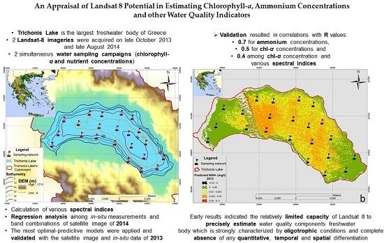
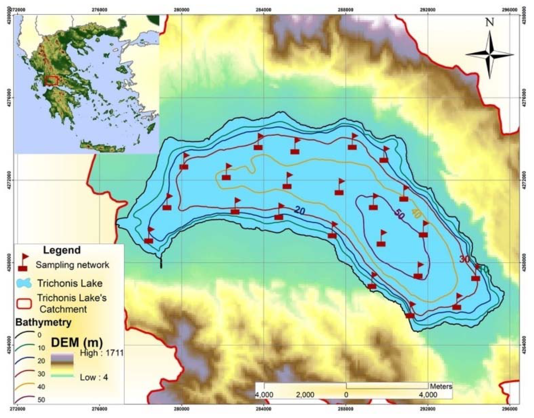
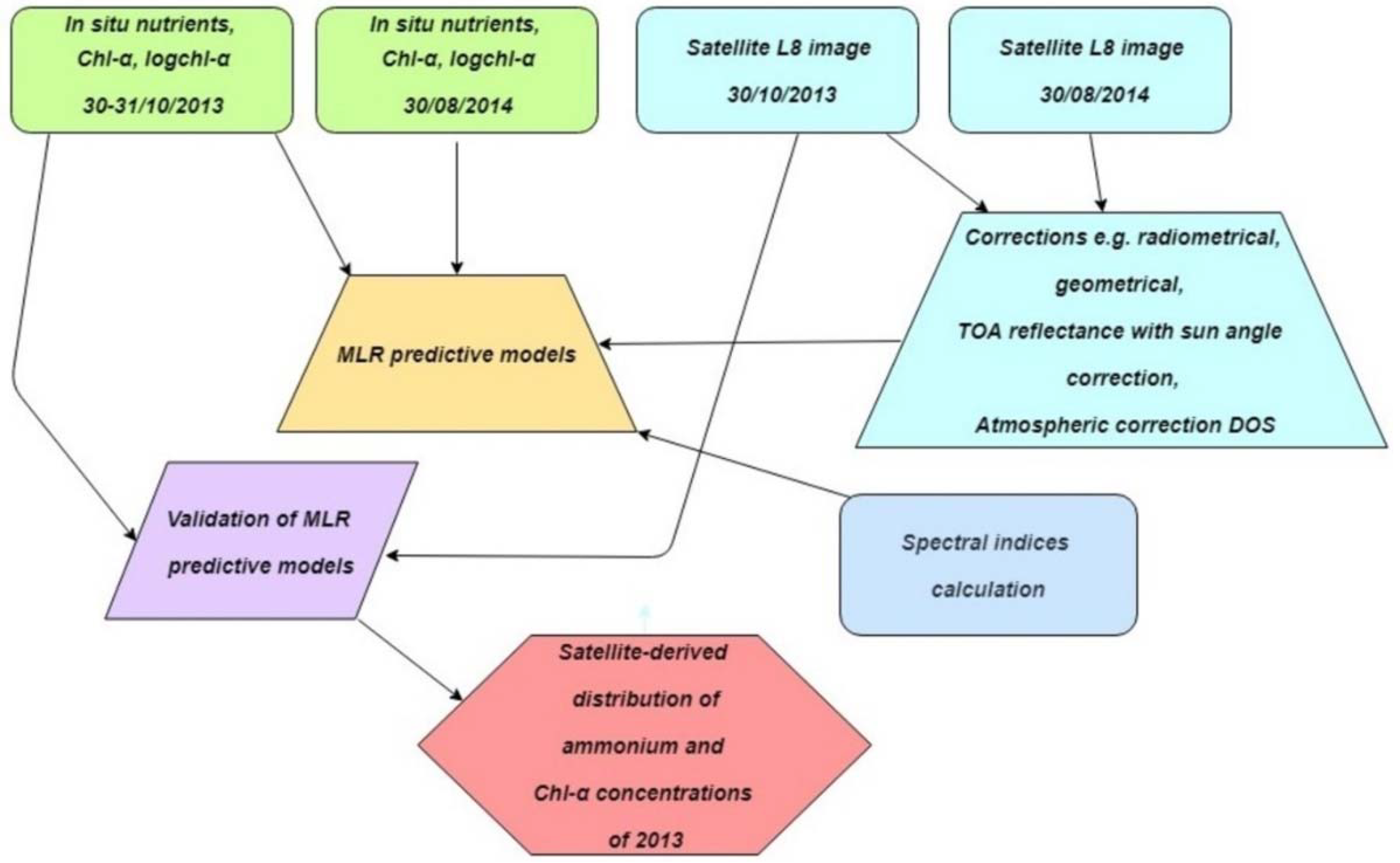
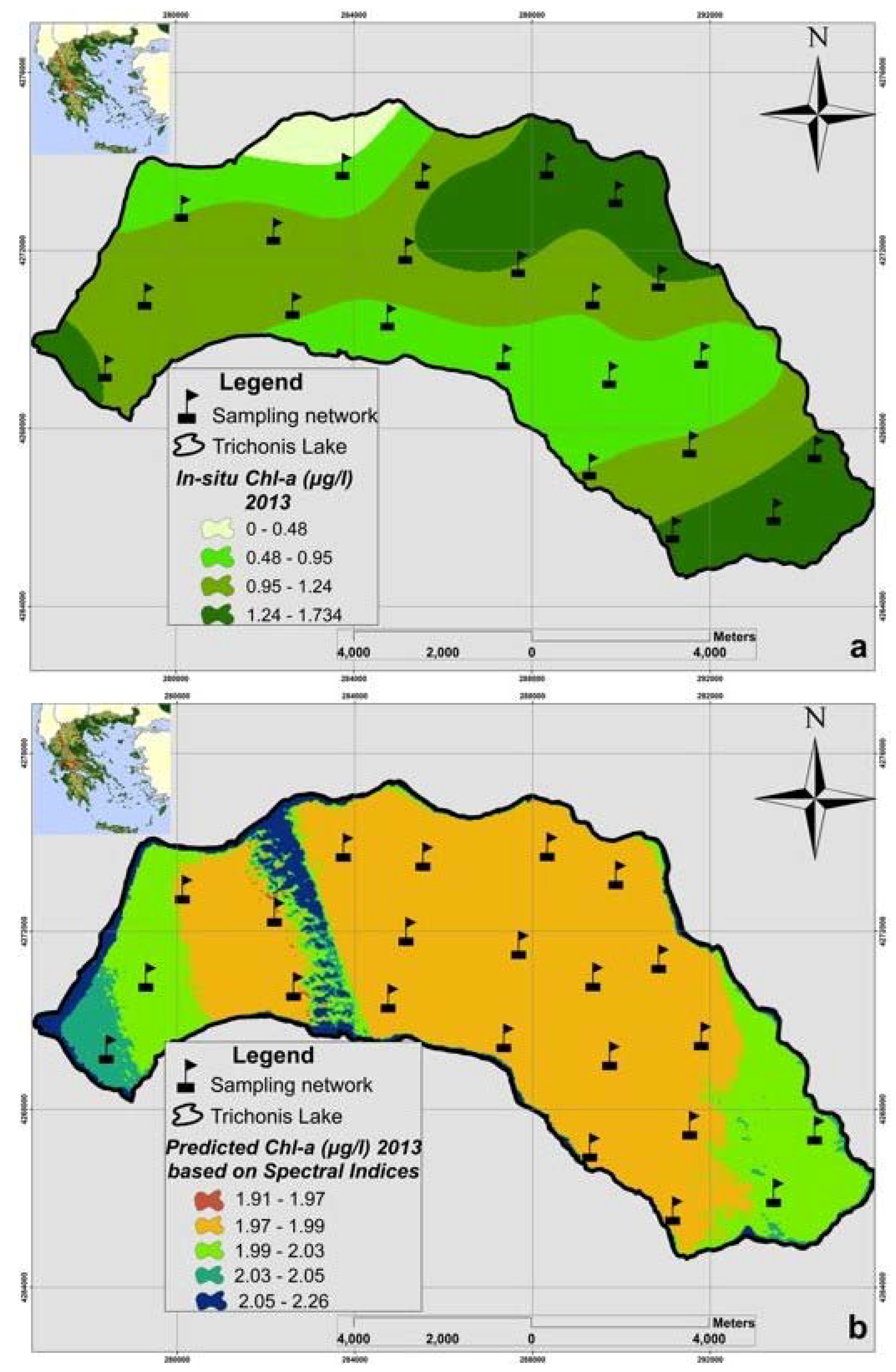
This study focuses on estimating lake water quality indicators such as Chlorophyll-a and the concentrations of nutrients through regression analysis among Landsat 8 surface reflectance and respective simultaneous in-situ data of the Trichonis lake for 2 dates. Acquisition dates of satellite and in-situ data were almost simultaneous, circumstances that favor the quality and accuracy of the processing results. To our knowledge, this is one of the few published studies concerned with the water quality monitoring of an oligotrophic freshwater body and on the monitoring of nutrients ‘concentrations, which are deprived of optical properties, a fact that makes elaboration through optical remote sensing a very challenging task. The main goal after the establishment of relations among the nutrients, chlorophyll-a concentrations and Landsat 8 observations using multiple linear regression, is the investigation of sensor’s effectiveness to accurately assess the water quality of Trichonida lake, the deepest and largest oligotrophic Lake of Greece.

2. Materials and Methods

2.1. Study Area

Trichonis Lake, the largest and deepest lake in Greece, is situated in the Aitoloakarnania Region of Western Greece. The lake’s surface area is 97 km2, its length 21 km, its greatest width 6.5 km and its potential water volume approximately 2.8 × 10⁹ m3 (Figure 1). Trichonis Lake shows significant annual and monthly water level fluctuations (~1 m and 0.5 m respectively). This is due to the variability in the climatic conditions as well as the implemented management practices [39]. The maximum depth is about 57 m while its trophic status is oligotrophic, exhibiting thermal stratification and orthograde distribution of dissolved oxygen [40] in [41]. High groundwater inflows have been detected during dry periods [42]. The regional climate is characterized as semi-arid to arid Mediterranean with an average annual rainfall of 936 mm and an average annual temperature of 17 °C which fluctuates by 19 °C annually [43]. The Trichonis Lake’s catchment consists of 399 km2 of semi-mountainous area. Its geology comprises mainly of calcareous formations with high permeability in the north and east parts while low permeability flysch formations are encountered in the south and west sections of the basin. Moreover, alluvial deposits and pleistocenic sediments lie around the lake [39].

2.2. Water Sampling, Chemical Analyses and EPA Quality Classification System

Water samples were collected from 22 stations across Trichonis Lake (Figure 1) on 30 October 2013 (15:00–18:00—9 stations), 31 October 2013 (12:00–16:00—rest stations) and 30 August 2014 (10:00–15:00—all stations). Following collection, the samples for nutrient analysis were preserved by the addition of HgCl2 and on return to the HCMR laboratories were filtered through 0.45 μm cellulose acetate filters that had been precleaned with 10% hydrochloric acid (pH = 2) followed by rinsing with Milli-Q water.
Water samples for chlorophyll-a were collected with NIO samplers and a specific quantity of water (usually 1 L) was filtered through Whatman GF/F filters immediately after collection. These filters were maintained in a dry and dark environment at −15 °C and then transferred to HCMR laboratories for further analysis [44].
Concentrations of nutrients (NO3, NO2, NH4+, PO43− and SiO44−) were determined in the soluble fraction using an ion analyzer Metrohm, the automatic analyzer Radiometer and the photometer Merck Nova 400. The chlorophyll-a concentrations were determined with a TURNER 00-AU-10U fluorometer according to the method of [45], modified by [46] in [44].
The EPA classification system was used for the water quality classification of Trichonis lake [47]. According to this scheme, total phosphorus concentration, water transparency and trophic index (Trophic State Index—TSI) determine the classification of lakes into six quality classes (Table 1). Trophic index TSI is calculated for each quality parameter as follows [48]:
TSI (SD) = 60 − 14.41 × ln(SD)
TSI (Chl-a) = 9.81 × ln(Chl-a) + 30.6
TSI (TP) = 14.42 × ln(TP) + 4.15
where SD is the Secchi disk (m) and Chl-a and TP (μg/L) are the concentrations of chlorophyll-a and total phosphorus, respectively.

2.3. Satellite Data Acqusition & Pre-Processing

A summary of the methodology adopted in this study is presented in Figure 2. Two Landsat 8 OLI images of Lake Trichonis (Path 184, Row 33) of 30 October 2013 (17:22:09Z) and 30 August 2014 (14:50:07Z) were acquired from the USGS (United States Geological Survey) Data Centre (http://glovis.usgs.gov/). More information about Landsat 8 OLI can be found in Table 2 or the USGS web site (https://landsat.usgs.gov).
ENVI (EXELIS Visual Information Solutions, Version 5.3) and ArcGIS (ESRI’s v. 10.1) software tools were used to process the acquired data. Both images were radiometrical and geometrically corrected (using GCPs) and a geometric accuracy of less than one half pixel (<15 m) was obtained. A top-of-atmosphere reflectance with sun angle correction was obtained in order to facilitate the comparison between multiple time periods. Equations (available at https://landsat.usgs.gov/using-usgs-landsat-8-product) were used to rescale the data based on sensor specific information and remove the effects of differences in illumination geometry. Additional information such as Earth-sun distance, solar zenith angle and exoatmospheric irradiance (all provided in the metadata file of each satellite image) are required. To compare the satellite-derived spectral properties of water and the in-situ measurements, the EO data were corrected for atmospheric effects (Humboldt University, on-line courses 2015) using the dark object subtraction (DOS) technique [20,49,50]. The basic principle of this method is that within the image there are some pixels that are completely shadowed and their radiances that are received at the satellite originate entirely from atmospheric scattering (path radiance). This radiance value is then being subtracted from each pixel value in the image. The largest sources of errors for water constituents’ retrieval are usually attributed to the bio-optical model that relates water leaving radiance (or reflectance) to the constituents’ concentrations and to treatment of aerosol reflectance in the atmospheric correction procedure [51].
Subsequently, several spectral (vegetation and water) indices were calculated (see Table 3 below) in order to assess chlorophyll-a concentrations.

2.4. Developing Relationships between Landsat 8 and Water Quality Data

There are several band combinations and transformations that have been proposed in the relevant literature in order to establish relationships between the Landsat 8 OLI reflectance data (independent) and chl-a, log(Chl-a), spectral indices and nutrient values (dependant). The possible consistent relationships between the water quality parameters and the satellite surface reflectance values of Landsat 8 image of 2013 and 2014 were examined via a multiple linear regression technique. In particular, the predictor importance chart (IBM SPSS software Statistics v. 23.0, Armonk, NY, USA) indicated the highest important predictors. Then those variables/predictors were further elaborated via numerous stepwise and backward linear regressions by being added and removed while examining for statistical performance and residuals. Further criteria such as multicollinearity, tolerance factor, variance inflation factor (VIF) and condition indices (CI) were applied and checked to a subset of optimal models in order to further compare them and select the most straightforward models instead of complicated ones with higher accuracy (higher R).
In addition to the above, several vegetation and water indices (Table 3) were calculated and added to the analysis (Figure 2). The usefulness of water indices has been demonstrated in different studies for drought monitoring and early warning assessment [59,60,61,62]. However, the vegetation indices and reflectance values (individuals bands and band ratios) application are highly encouraged for the estimation of water quality parameters (i.e., chlorophyll-a, transparency) in lakes [63,64,65,66] in [62]. As a last step of the analysis, the most accurate regression models (developed by satellite and in-situ data of August 2014) were selected on the basis of the established statistical criteria described earlier on, while then they were validated based on the satellite and in-situ data of 2013.

3. Results

3.1. Statistical Summary of Trichonis Lake’s In-Situ Measurements and EPA Water Quality Classification

In-situ concentrations of nitrate, nitrite, phosphate and total nitrogen were measured in 2014 as lower than each respective detection limit of the photometer Merck Nova 400, hence those data were not statistically elaborated. Data distributions for the rest parameters were skewed with mostly low values and without extremely high values or outliers (Table 4). Chlorophyll-a concentrations ranged from 0.5 to 1.4 μg/L with mean value 1.07 μg/L during the sampling campaign of 2013 and between 0.2 and 0.9 μg/L with average value 0.39 μg/L in 2014. Mean values of total phosphorus indicate the presence of similar conditions into the lake since those values for both years are equal to 0.04 and 0.02 mg/L for 2013 and 2014, respectively (Figure 3 and Figure 4b).
Ammonium concentrations demonstrated even more resembling values, which ranged from 0.02 to 0.06 mg/L in 2013 and from 0.01 to 0.09 mg/L in 2014, with identical mean value equal to 0.03 mg/L. In general, concentrations of chlorophyll-a and total phosphorus were measured slightly higher in 2013 than the values of 2014 compared to ammonium concentrations (Figure 3 and Figure 4a,b). Those values though are slightly increased, thus no water quality deterioration is indicated in 2013. Taking into account the values of coefficient of variation (CV %), it is observed that for all the three studied parameters the CV % is greater in 2014 than in 2013, whereas CV % of TP and NH4+ in 2014 are measured almost as double compared to Chl-a concentrations.
Regarding the EPA classification system, chlorophyll-a and phosphorus concentrations were utilized in order to classify the water quality of Trichonis Lake. This preliminary classification contributed to better understanding of the prevailing conditions during the sampling periods and assured that the trophic status is indeed oligotrophic. Thus, after having assessed the Carlson Trophic Index for Chl-a and TP, average values of Carlson Trophic State Index (average TSI) were used in order to classify the trophic status of Trichonis Lake (Table 5).

3.2. MLR Analysis and Predictive Models

Analysis concerning the in-situ data of 2013 and L8 band combinations of the respective date returned statistical results though were not significant. Taking into account the correlations accompanied by the greatest values of correlation coefficient, correlation analysis was subsequently attempted between the in-situ data of 2013 and mean remote sensed values. Those values were retrieved from 90 m buffer zones that were created around each sampling station and were transformed into surface reflectance. The retrieval of a mean reflectance value around each in situ sampling site was considered more appropriate in order to reduce sensor and algorithm noise [67]. Those results were equally statistically not significant. Subsequently, the in-situ data of 2014 were correlated with band combinations of satellite image of 2014. This correlation analysis, after having tested more than 45 band combinations, yielded more statistically acceptable results compared to data of 2013.
Multiple linear regression analysis among satellite and in-situ data of 2014 resulted in moderate and low correlations. Low and statistically insignificant relationships were detected particularly among reflectance values and total phosphorus concentrations while the most remarkable (but still statistical insignificant) results, are presented below (Table 6). Total phosphorus’s predictive model 1 yielded R and R2 values equal to 0.27 and 0.07, respectively while the predictors included are the subtraction between bands 3 and 4 and the natural logarithm of B4 and B3 ratio (Table 7). Then, using the backward linear regression, ln (B4/B3) was removed (Table 7) and predictive model 2 resulted in R and R2 values equal to 0.24 and 0.06, respectively while Durbin-Watson’s statistic indicates an absence of autocorrelation in the residuals (Table 7). Taking into account certain statistical indices (especially the value of R2), all predictive models of total phosphorus were rejected due to their low performance.
The spatial distribution of spectral indices, measured from satellite image of 2014, also indicated slight differences and variance (Table 8). Moreover, the greatest value range is apparent in NDVI values (0.0227) while the lowest is in the EVI index. Regarding all indices, no great difference is detected in maximum and minimum values, indicating once again the great spatial homogeneity and the lack of variability that characterizes Trichonis Lake.
Spectral indices, involving mostly red and near infrared bands, indicated weak relationships. A regression analysis was developed among spectral indices chlorophyll-a concentrations and log(chl-a) and the most optimal model was established among logchl-a values and spectral indices. For the logchl-a model, 4 equations were evaluated, with the following independent variables: the EVI, NDWI, MNDWI and NDVI vegetation and water indices (Table 9).
According to the predictor importance chart (Figure 5a) and the regression analysis results between chl-a concentrations and the spectral bands combinations, factors B2/(B1 + B2 + B3) and (B1 + B2)/2 indicated one optimal predictive model (Table 10).
Taking into account certain statistical indices (predictor importance chart, R, tolerance factor, VIF, CI, Durbin-Watson, and absolute and relative RMSE) final optimal predictive models were documented for each in-water quality constituent (Table 10). MLR model involving Landsat 8 bands 1 (ultra-blue), 3 (green), 4 (red) and their combination (Figure 5b) proved to be the most suitable for predicting ammonium concentrations in Trichonis Lake. Coefficient of correlation equals to 0.3 while Durbin-Watson value indicates independence of residuals. As such, the best predictive model for the estimation of chlorophyll-a concentration incorporates Landsat 8 bands B2/(B1 + B2 + B3) and (B1 + B2)/2, accompanied by a correlation coefficient equal to 0.44. Collinearity statistics (Tolerance and VIF) of the coefficients are 0.964 and 1.04, respectively excluding the possibility of multicollinearity. Concerning the logchl-a predictive model, vegetation and water spectral indices EVI, NDWI, MNDWI and NDVI were used presenting marginally acceptable statistics (Table 10). Chlorophyll-a can be measured initially by using vegetation indices and by extension based on the green and SWIR bands of water indices (NDWI, MNDWI) due to chlorophyll-a absorbance in violet-blue and orange-red wavelengths and its reflection in green/yellow light.

3.3. Algorithm Validation

The reliability and validation of the final selected models was investigated based on statistical indices, resulted from the implementation of several regression models among Landsat 8-estimated values of Chl-a, logchl-a and ammonium concentrations in Trichonis Lake and their respective in-situ values of 2013. Linear, logarithmic, quadratic, cubic, power and exponential models, have been developed among the observed (in situ) data of 2013 and satellite derived data in order to detect the best potential agreement and performance and by extension to validate the final selected assessment models During this validation process, regression analysis indicated the cubic model as the model with the highest correlation coefficients for all the under study parameters (chl-a, ammonium), except for logchl-a where the quadratic model was proven to yield slightly better results than the cubic one (Table 11). Nevertheless, the low performance (low R and R2 values) and poor fit of the aforementioned validation models imply their moderate-to low predictive potential and more in-situ data are required in order to train more effective algorithms. Besides, the highest correlation coefficient among all validation models, is associated with the ammonium concentration assessment model and it is equal to 0.7, then follows chl-a cubic model with R equal to 0.5 and finally logchl-a predictive model with similar values between cubic and quadratic models, 0.4 and 0.41, respectively (Table 11).
The spatial distribution of in-situ measurements of NH4+ (Figure 6a) and Chl-a concentration (Figure 7a and Figure 8a) was mapped through their spatial interpolation using the Spline method in order to compare the output with the satellite derived values. Other interpolation methods, such as IDW (Inverse Distance Weighted) and natural neighbor, were also tested, but Spline method generated the smoothest surfaces and representative values that were closer to the in-situ measured concentrations. The ammonium assessment model was selected to be depicted as the model with the highest correlation coefficient (validation process) and its application on the satellite image of 2013 yielded concentrations which range from 0 to 0.11 mg/L (Figure 6b) in relation to in-situ ammonium distribution which ranged from 0 to 0.08 mg/L (Figure 6a). Pixels having negative values were deleted and the few that remained are illustrated with a black color.
Furthermore, the application of the predictive models on the satellite data of 2013 indicated some increasing or decreasing assessment trends compared to the respective in-situ data. In particular, chl-a predictive models overestimated the actual chl-a concentrations, with the main difference being that the model retrieved from singe band combinations presents a more fluctuated value distribution (Figure 7b) than the Chl-a retrieved from specific spectral indices (Figure 8b). On the other hand, ammonium concentrations are slightly underestimated compared to in-situ, while the assessment model managed to predict the exact value at the T8 sampling station (Figure 9c). Moreover, it is observed that predicted ammonium concentrations follow, in general, similar distribution with the respective in-situ, concerning the value fluctuations. An exception is obvious at T14 sampling station, where in-situ values illustrate an increase and the greatest value while at the same point predicted ammonium presents a decrease and the lowest value, respectively.

4. Discussion

The possibility of providing large scale and high frequency data makes the use of remote sensing technology a suitable approach for tracking phenomena at a temporal scale suitable to the development of the event. This is true, for example, for algal blooms, since the traditional limnological surveys are inadequate and expensive. Moreover, satellite data are key pieces of information for monitoring the effect of climate change. Climate related-factors, such as the amount and intensity of rainfall affecting the basin runoff, can have major effects on the availability of nutrients for algae in lakes. Limnology can benefit from techniques that allow the collection, in near real time, of large scale data, thus accomplishing a better understanding of the response of lacustrine ecosystem to peculiar meteorological events related to climate change [6]. Unfortunately, in this study, the limited potential of Landsat 8 OLI imagery to accurately determine water quality parameters’ concentrations (chl-a and nutrients) in an oligotrophic waterbody was demonstrated.
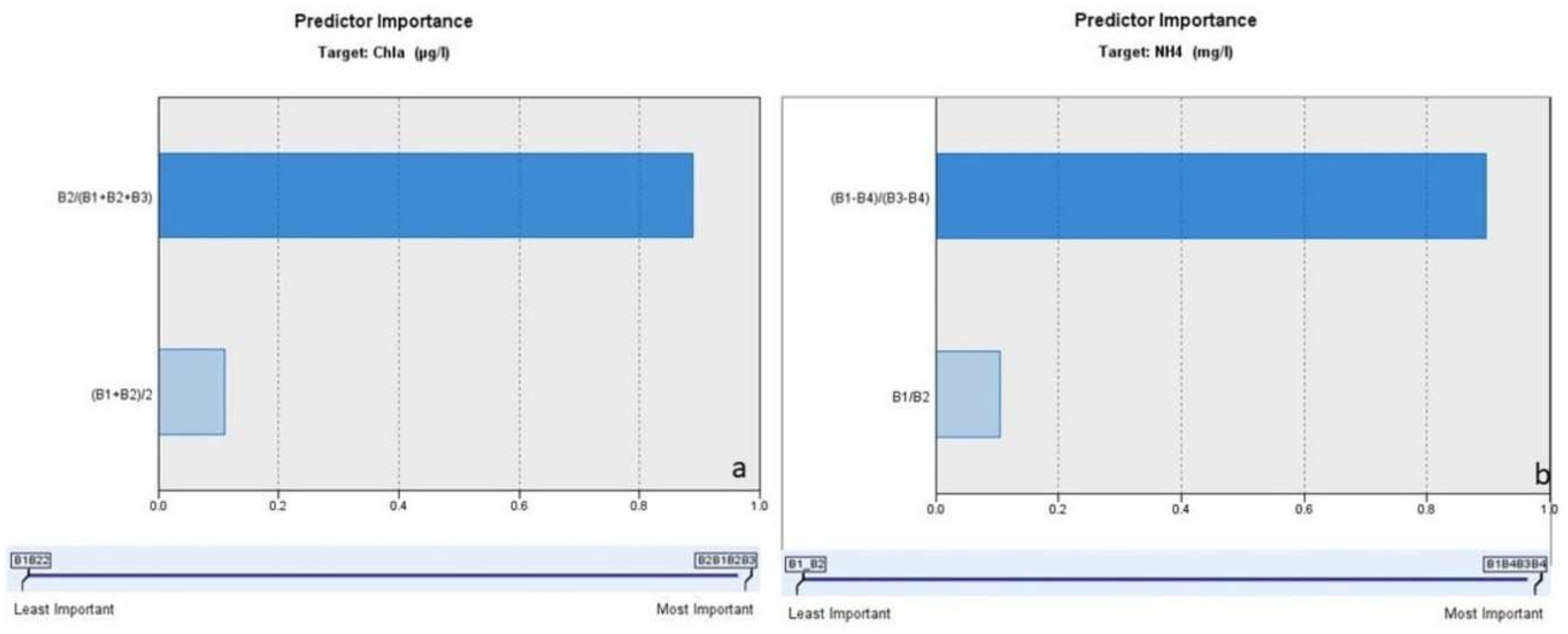
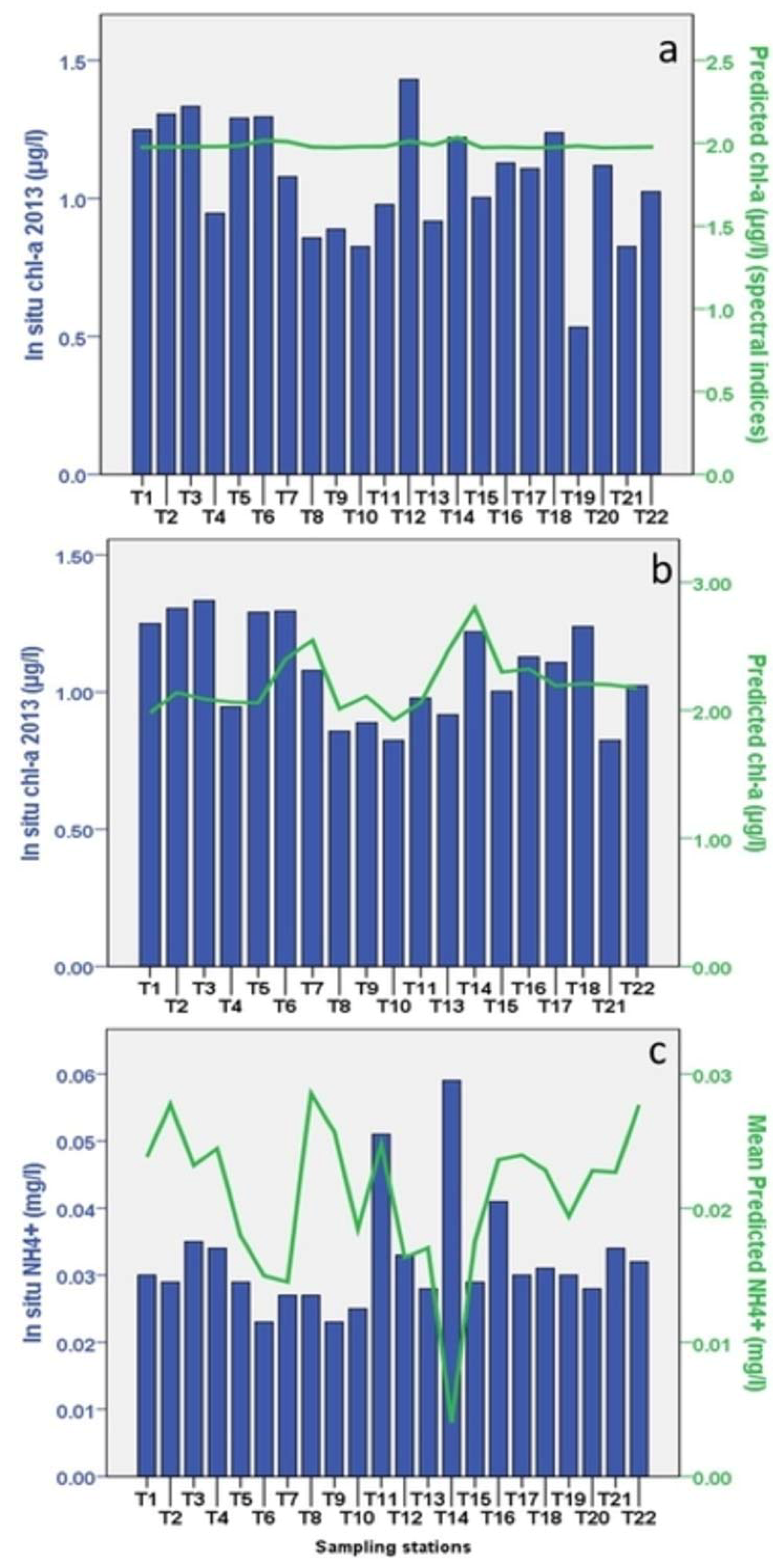
Several multiple linear regressions were established yielding insignificant statistical correlations among satellite and in-situ data. The final chl-a algorithm based on single Landsat bands, includes the bands B1 (ultra blue), B2 (blue) and B3 (green) [68] mapped OLI’s spectroradiometric sensitivity to changes in optically active components (OACs), for a nominal solar zenith angle θs = 40°, while the solar zenith angle in our study equals to θs = 35°. According to [68], for chl-a changes greater than 0.5 μg/L, the blue band demonstrates the highest sensitivity. This indicates some disadvantages in detecting changes smaller than 0.5 μg/L (usually in oligotrophic waters). Furthermore, B1 was proven to yield better results in waters with relatively low chl-a concentrations while B3 usually demonstrates similar sensitivity with B1.
Nutrient concentrations are in-water quality components that lack optical properties. This is the most significant reason that so few studies have not only attempted to map them but also actually managed to monitor them accompanied by reliable statistical results. Moreover, very few are the projects that were able to establish total nitrogen algorithms with statistically significant results or reasonable adjusted R2 values [24]. Based on our study, the final ammonium algorithm involved the B1, B3 and B4 bands associated with a regression coefficient equal to 0.7, as far as the validation process is concerned. Studies by [26] and [24] utilized Landsat TM bands and demonstrated similar outcomes, by using bands 1 (blue) and 2 (green). On the other hand, although Reference [25] predicted total nitrogen concentrations by using Landsat TM bands 1 (blue), 2 (green), 3 (red), and 4 (NIR), those were not very successful (R2 = 0.24) [24].
According to our study findings, the logchl-a predictive model based on spectral indices incorporated OLI bands 2 (blue), 3 (green), 4 (red), 5 (NIR) and 7 (swir2) with R equal to 0.58 [13,16,62,69] used similar bands for the estimation of chlorophyll-a in lakes and reservoirs and more particular vegetation indices and bands TM and ETM 1 (blue), 2 (green) and 4 (NIR). Reference [62] used the NDVI in Laguna Chascomús in relation to Chl-a estimation for its optical characteristics and because it is sensitive to the pigment absorption. NDVI has been found to be very sensitive to changes in the environment [62,63]. Moreover, its use is more successful in zones with moderate wind speeds without developing waves, which is not the case in Trichonis Lake [62]. Furthermore, water indices include SWIR band and according to Reference [70] all significant band combinations for chlorophyll included at least one of the short wave infrared bands (SWIR), although most water quality studies to this point have not included SWIR bands. Ratios between either chlorophyll absorption bands (red and blue) or chlorophyll reflectance bands (green and NIR) with either of the two SWIR bands expected to emphasize the portion of the spectrum affected by chlorophyll, thereby making estimated values more readily correlated with actual sample values [70]. Reference [71] also tried to generate a different Chl-a model for different Landsat sensors (5 TM, 7 ETM+ and 8 OLI). Although OLI sensor has better radiometric sensitivity and signal to noise ratio, they could not prove that OLI is better than TM and ETM+ sensors. Overall, they observed that each Landsat sensor can be used to estimate Chl-a in the reservoir while the best model for TM sensor included a combination of green, red and NIR band, and the ratio green/red (R2 = 0.92). A three-variable model using green and SWIR-1 bands and the ratio red/green was the best model to predict Chl-a using EMT+ sensor (R2 = 0.91).
Effective and precise water quality determination is dependent on the satellite sensor used, the methodology followed and also on the nature of the waters studied (Case-1, Case-2). Based in these premises the aforementioned authors (who used Landsat images) in addition to [72,73], concluded that the application of MERIS FLH algorithms in oligotrophic waters may be excluded because of too low signal to noise ratio. Furthermore, according to Reference [74], eutrophic and mesotrophic lakes provide more accurate estimations than oligotrophic, due to the lack of suspended particles that are detectable by satellite sensors.
All in all, in this study results showed that water quality monitoring of oligotrophic freshwater bodies through remote sensing tools can be a really challenging task. Landsat 8 has been widely used in eutrophic lakes and even fewer studies have managed to estimate nutrients, particularly ammonium concentrations. Season of water samplings, lake trophic status and the spatial homogeneity may be the greatest limitations that prevented a better and more accurate prediction. In case of a better performance of predictive models, the continuous water quality monitoring of Trichonis lake would be feasible in combination with simultaneous satellite imageries. Those models might be extended and applied efficiently in other lakes of the planet with similar morphological characteristics, contributing to cost savings, knowledge dissemination regarding lake management and protection and implementation of recovery strategies.

5. Conclusions

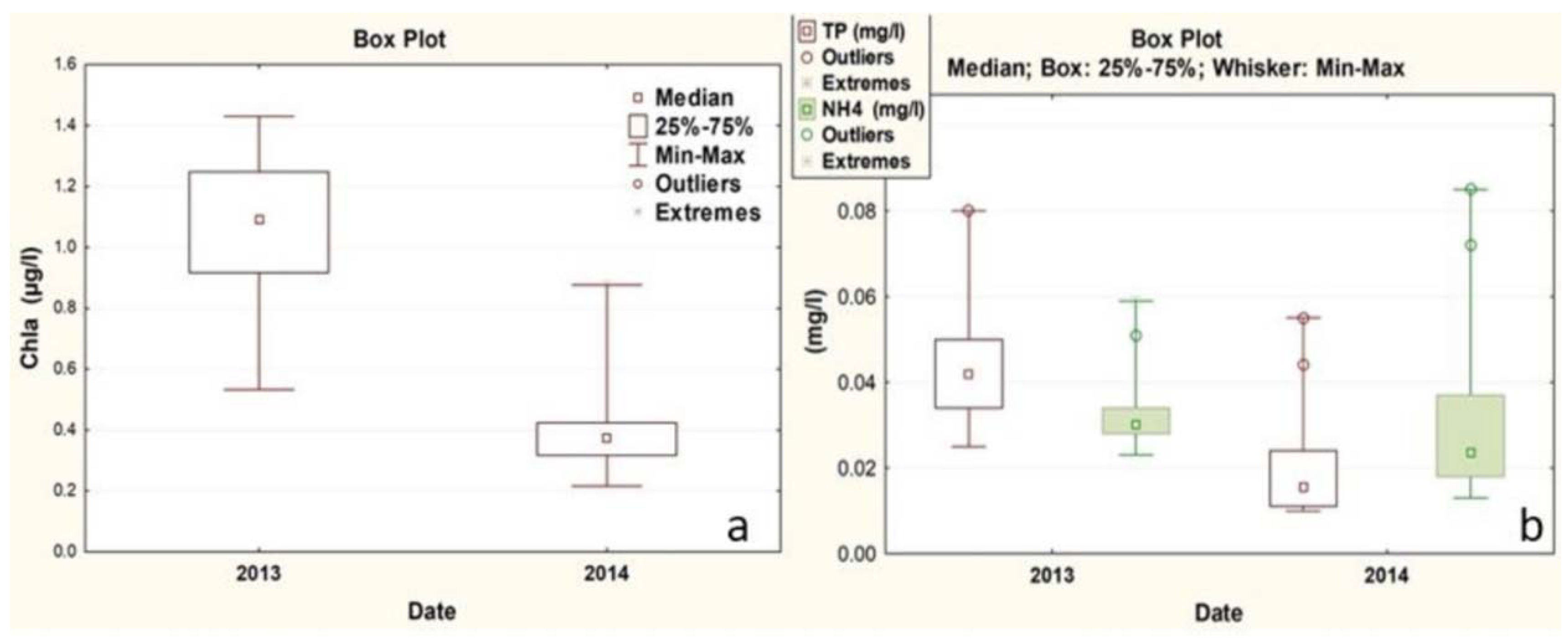
Our study explored the use of remote sensing technology and specifically of Landsat 8 OLI sensor, to accurately quantify certain water quality parameters. Two water sampling campaigns were conducted in the largest and deepest lake of Greece, Trichonis Lake, in 2013 and 2014 studying concentrations of chlorophyll-a and nutrients while simultaneous L8 imageries were at our disposal. Although chlorophyll-a is broadly used as a lake water quality indicator in combination with satellite data, very few studies have investigated the prediction of nutrient concentrations.
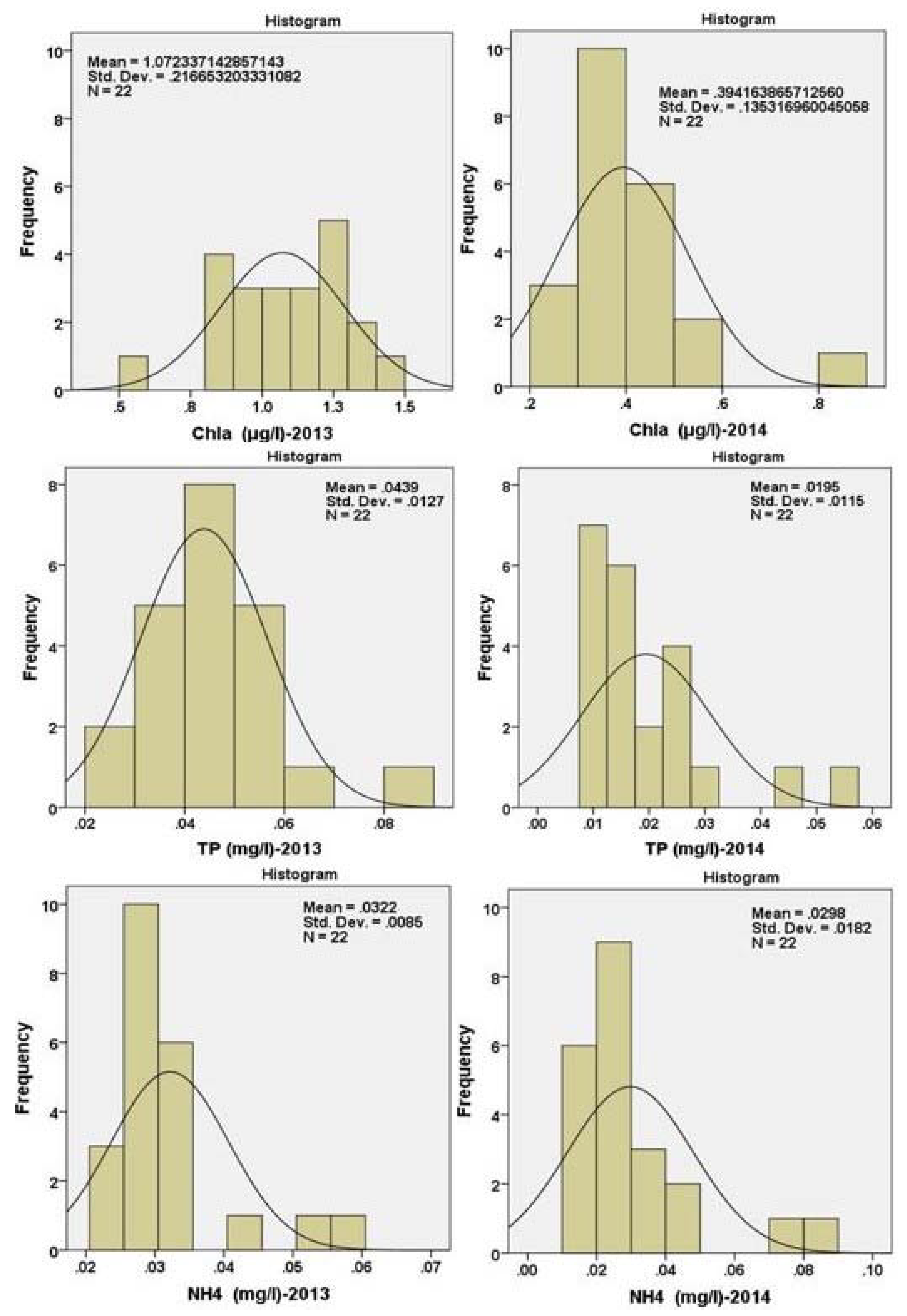
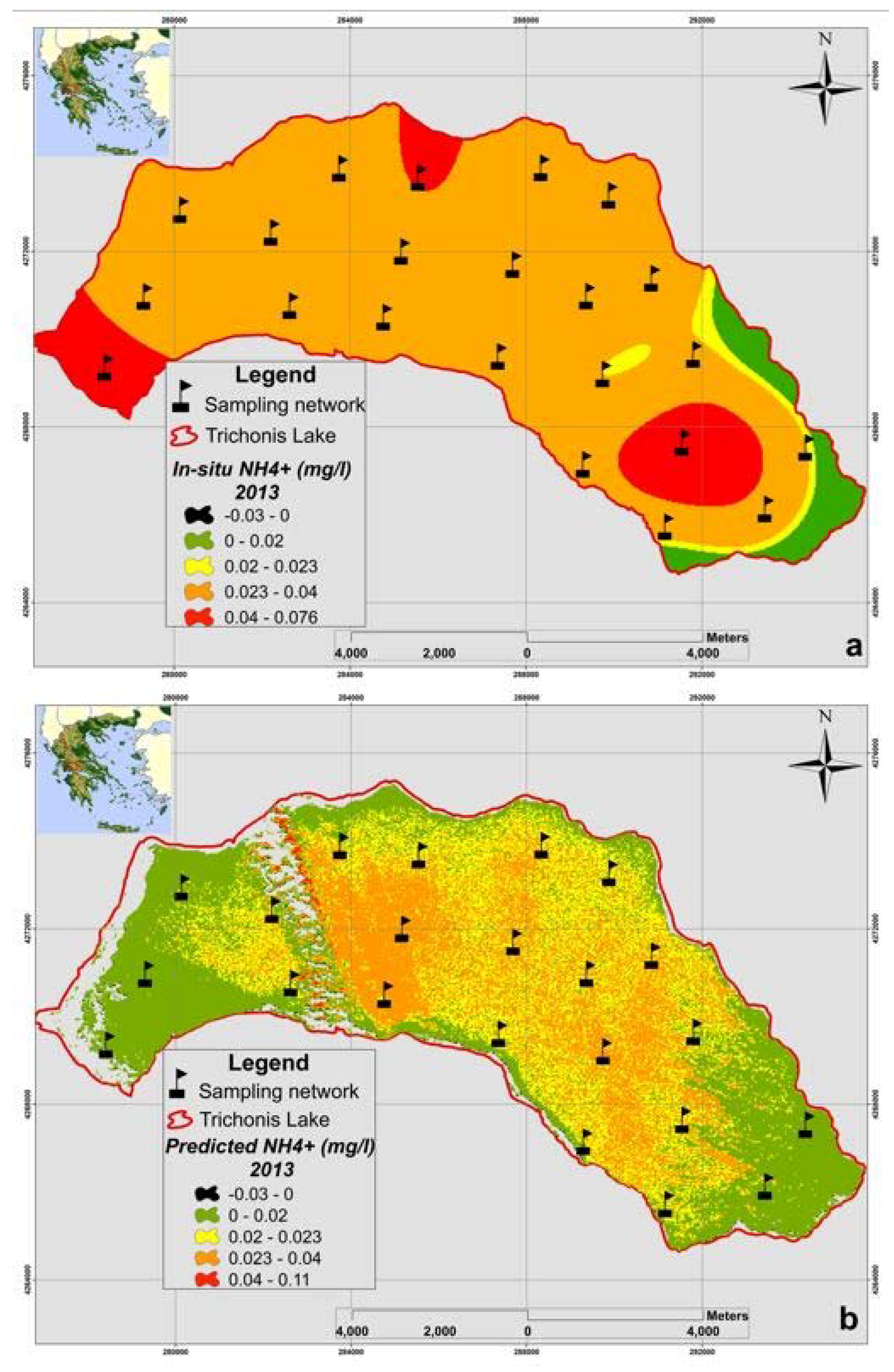
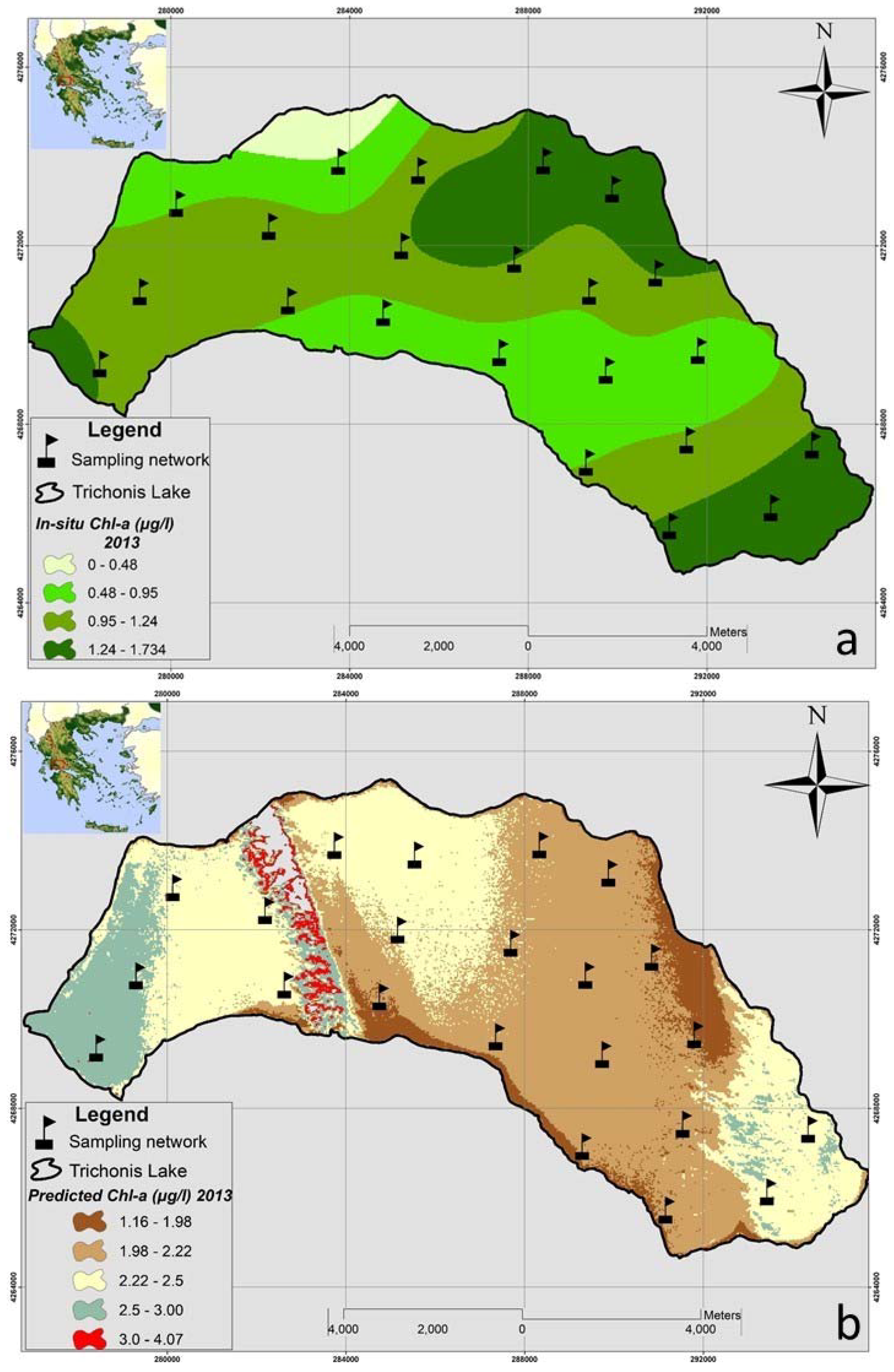
According to the in-situ data analysis and their spatial distribution, it has been strongly ascertained that Trichonis Lake is characterized by particularly low concentrations and the lack of any spatial or temporal value differentiation across the twenty-two sampling stations, case that inhibited a greater predictive potential. Weak correlations were detected among in-situ and satellite data while those correlations, particularly in autumn and summer, may also be due to the lake turnover effect. When the equalization of the thermal gradient in the lake induces mixing of surface and bottom waters, remote monitoring is made difficult due to instability [70].
Moreover, the incorporation of the SWIR band into chl-a estimation (in contrast to other studies) suggests that there may be a relationship between SWIR reflection and algae/plant production, which deserves further investigation. Additional water samplings should be made during different time periods concerning specific mixing boundaries (surface-bottom waters) in order to investigate whether the feasibility of remote monitoring increases. In case strong relationships are found, this may help improve prediction capabilities by providing researchers with bounded time periods (according to region) [70]. Further research is required towards the investigation of more water parameters or using sensors of different spatial and geometrical analysis in order to be able to compare the outcomes among all different cases. Even though early results demonstrated the vulnerability of the Landsat 8 imagery to precisely determine certain water quality components in an inland oligotrophic body, it is generally accepted that those models may initially increase the knowledge of Trichonis lake’s water quality and then be utilized as warning indicators of water quality deterioration.

Author Contributions

V.M. and E.D. conceived and designed the concept of the paper; V.M. analyzed the data and wrote the paper; D.K. contributed to statistical interpretations; G.P., D.K. and E.D. contributed to the paper revision.

Funding

GPP’s contribution has been supported by the FP7- People project ENViSIon-EO (project reference number 334533.

Conflicts of Interest

The authors declare no conflict of interest.

References

  1. Coppin, P.; Jonckheere, I.; Nackaerts, K.; Muys, B.; Lambin, E. Digital change detection methods in ecosystem monitoring: A review. Int. J. Remote Sens. 2004, 25, 1565–1596. [Google Scholar] [CrossRef]
  2. Vörösmarty, C.J.; Green, P.; Salisbury, J.; Lammers, R.B. Global water resources: Vulnerability from climate change and population growth. Science 2000, 289, 284–288. [Google Scholar] [CrossRef] [PubMed]
  3. Arnell, N.W. Climate change and global water resources: SRES emissions and socio-economic scenarios. Glob. Environ. Chang. 2004, 14, 31–52. [Google Scholar] [CrossRef]
  4. Alcamo, J.; Flörke, M.; Märker, M. Future long-term changes in global water resources driven by socio-economic and climatic changes. Hydrol. Sci. J. 2007, 52, 247–275. [Google Scholar] [CrossRef] [Green Version]
  5. Schewe, J.; Heinke, J.; Gerten, D.; Haddeland, I.; Arnell, N.; Clark, D.; Dankers, D.; Eisner, S.; Fekete, B.M.; Colón-González, F.J.; et al. Multimodel assessment of water scarcity under climate change. Proc. Natl. Acad. Sci. USA 2013, 111, 3245–3250. [Google Scholar] [CrossRef] [PubMed] [Green Version]
  6. Giardino, C.; Bresciani, M.; Stroppiana, D.; Oggioni, A.; Morabito, G. Optical remote sensing of lakes: An overview on Lake Maggiore. J. Limnol. 2014, 73, 201–214. [Google Scholar] [CrossRef] [Green Version]
  7. Kassymbekova, A.; Nessipbekov, G.; Yapiyev, V. Application of GIS and Remote Sensing techniques to analyze lake water balance in a sparsely gauged catchment: Case study Burabay National Nature Park, Kazakhstan A. In Proceedings of the 15th World Lake Conference, Perugia, Italy, 1–5 September 2014; Volume 2. [Google Scholar]
  8. Poikane, S.; Alves, M.H.; Argillier, C.; Berg, M.; Buzzi, F.; Hoehn, E.; de Hoyos, C.; Karottki, I.; Laplace-Treyture, C.; Solheim, A.L.; et al. Defining chlorophyll-a reference conditions in European lakes. Environ. Manag. 2010, 45, 1286–1298. [Google Scholar] [CrossRef] [PubMed] [Green Version]
  9. Huo, S.; Xi, B.; Su, J.; Zan, F.; Chen, Q.; Ji, D.; Ma, C. Determining reference conditions for TN, TP, SD and Chl-a in eastern plain ecoregion lakes, China. J. Environ. Sci. 2013, 25, 1001–1006. [Google Scholar] [CrossRef]
  10. Randolph, K.; Wilson, J.; Tedesco, L.; Li, L.; Pascual, D.L.; Soyeux, E. Hyperspectral remote sensing of cyanobacteria in turbid productive water using optically active pigments, chlorophyll-a and phycocyanin. Remote Sens. Environ. 2008, 112, 4009–4019. [Google Scholar] [CrossRef]
  11. Ruiz-Verdu, R.; Koponen, S.; Heege, T.; Doerffer, R.; Brockmann, C.; Kallio, K.; Pyhälahti, T.; Pena, R.; Polvorinos, Á.; Heblinski, J.; et al. Development of MERIS Lake Water Algorithms: Validation Results from Europe. In Proceedings of the 2nd MERIS/(A)ATSR User Workshop, Frascati, Italy, 22–26 September 2008. [Google Scholar]
  12. Stadelmann, T.H.; Brezonik, P.L.; Kloiber, S.M. Seasonal patterns of chlorophyll-a and Secchi disk transparency in lakes of east-central Minnesota: Implications for design of ground and satellite-based monitoring programs. Lake Reserv. Manag. 2001, 17, 299–314. [Google Scholar] [CrossRef]
  13. Olmanson, L.G.; Bauer, M.E.; Brezonik, P.L. A 20-year Landsat water clarity census of Minnesota’s 10,000 lakes. Remote Sens. Environ. 2008, 112, 4086–4097. [Google Scholar] [CrossRef]
  14. Papoutsa, C.; Retalis, A.; Toulios, L.; Hadjimitsis, D.G. Defining the Landsat TM/ETM+ and CHRIS/PROBA spectral regions in which turbidity can be retrieved in inland waterbodies using field spectroscopy. Int. J. Remote Sens. 2014, 35, 1674–1692. [Google Scholar] [CrossRef]
  15. Tyler, A.N.; Svab, E.; Preston, T.; Presing, M.; Kovacs, A.W. Remote sensing of the water quality of shallow lakes: A mixture modeling approach to quantifying phytoplankton in water characterized by high-suspended sediment. Int. J. Remote Sens. 2006, 27, 1521–1537. [Google Scholar] [CrossRef]
  16. Brezonik, P.; Menken, D.; Bauer, M. Landsat-based remote sensing of lake water quality characteristics, including chlorophyll and colored dissolved organic matter (CDOM). Lake Reserv. Manag. 2005, 21, 373–382. [Google Scholar] [CrossRef]
  17. Karakaya, N.; Evrendilek, F.; Aslan, G.R.; Gungor, K.; Karakas, D. Monitoring of lake water quality along with trophic gradient using landsat data. Int. J. Environ. Sci. Technol. 2011, 8, 817–822. [Google Scholar]
  18. Tebbs, E.J.; Remedios, J.J.; Harper, D.M. Remote sensing of chlorophyll-a as a measure of cyanobacterial biomass in Lake Bogoria, a hypertrophic, saline–alkaline, Flamingo Lake, using Landsat ETM+. Remote Sens. Environ. 2013, 135, 92–106. [Google Scholar] [CrossRef]
  19. Torbick, N.; Feng, H.; Zhang, J.; Qi, J.; Zhang, H.; Becker, B. Mapping chlorophyll-a concentrations in West Lake, China using Landsat 7 ETM+. J. Gt. Lakes Res. 2008, 34, 559–565. [Google Scholar] [CrossRef]
  20. Vincent, R.K.; Qin, X.; McKay, R.M.L.; Miner, J.; Czajkowski, K.; Savino, J.; Bridgeman, D. Phycocyanin detection from LANDSAT TM data for mapping cyanobacterial blooms in Lake Erie. Remote Sens. Environ. 2004, 89, 381–392. [Google Scholar] [CrossRef]
  21. Yacobi, Y.Z.; Gitelson, A.; Mayo, M. Remote sensing of chlorophyll in Lake Kinneret using high spectral-resolution radiometer and Landsat TM: Spectral features of reflectance and algorithm development. J. Plankton Res. 1995, 17, 2155–2173. [Google Scholar] [CrossRef]
  22. Zhou, W.; Wang, S.; Zhou, Y.; Troy, A. Mapping the concentrations of total suspended matter in lake Taihu, China, using Landsat-5 TM data. Int. J. Remote Sens. 2006, 27, 1177–1191. [Google Scholar] [CrossRef]
  23. Albright, T.P.; Ode, D.J. Monitoring the dynamics of an invasive emergent macrophyte community using operational remote sensing data. Hydrobiologia 2011, 661, 469–474. [Google Scholar] [CrossRef]
  24. Isenstein, E.M.; Park, M.-H. Assessment of nutrient distributions in Lake Champlain using satellite remote sensing. J. Environ. Sci. 2014, 26, 1831–1836. [Google Scholar] [CrossRef] [PubMed]
  25. Chen, J.; Quan, W.T. Using Landsat/TM imagery to estimate nitrogen and phosphorus concentration in Taihu Lake, China. IEEE J. Sel. Top. Appl. Earth Obs. Remote Sens. 2012, 5, 273–280. [Google Scholar] [CrossRef]
  26. Dewidar, K.; Khedr, A. Water quality assessment with simultaneous Landsat-5 TM at Manzala Lagoon, Egypt. Hydrobiologia 2001, 457, 49–58. [Google Scholar] [CrossRef]
  27. Wu, F.; Wu, J.P.; Qi, J.G.; Zhang, L.S.; Huang, H.Q.; Lou, L.P.; Chen, Y. Empirical estimation of total phosphorus concentration in the mainstream of the Qiantang River in China using Landsat TM data. Int. J. Remote Sens. 2010, 31, 2309–2324. [Google Scholar] [CrossRef] [Green Version]
  28. Yang, Z.; Reiter, M.; Munyei, N. Estimation of chlorophyll-a concentrations in diverse water bodies using ratio-based NIR/Red indices. Remote Sens. Appl. Soc. Environ. 2017, 6, 52–58. [Google Scholar] [CrossRef]
  29. Pierson, D.; Strombeck, N. A modeling approach to evaluate preliminary remote sensing algorithms: Use of water quality data from Swedish great lakes. Geophysica 2000, 36, 177–202. [Google Scholar]
  30. Song, K.S.; Li, L.L.; Tedesco, S.; Li, H.; Duan, T.; Liu, D.W.; Hall, B.; Du, J.; Li, Z.C.; Shi, K.; et al. Remote estimation of chlorophyll-a in turbid inland waters: Three-band model versus GA-PLS model. Remote Sens. Environ. 2013, 136, 342–357. [Google Scholar] [CrossRef]
  31. Sun, D.; Hu, C.; Qiu, Z.; Cannizzaro, J.P.; Barnes, B.B. Influence of a red band-based water classification approach on chlorophyll algorithms for optically complex estuaries. Remote Sens. Environ. 2014, 155, 289–302. [Google Scholar] [CrossRef]
  32. Huang, C.; Zou, J.; Li, Y.; Yang, H.; Shi, K.; Li, J.; Chena, X.; Zheng, F. Assessment of NIR-red algorithms for observation of chlorophyll-a in highly turbid inland waters in China. ISPRS J. Photogramm. Remote Sens. 2014, 93, 29–39. [Google Scholar] [CrossRef]
  33. Yang, W.; Matsushita, B.; Chen, J.; Fukushima, T.; Ma, R.H. An enhanced three band index for estimating chlorophyll-a in turbid case-II waters: Case studies of Lake Kasumigaura, Japan, and Lake Dianchi, China. IEEE Geosci. Remote Sens. Lett. 2010, 7, 655–659. [Google Scholar] [CrossRef] [Green Version]
  34. Le, C.; Li, Y.; Zha, Y.; Sun, D.; Huang, C.; Lu, H. A four-band semi-analytical model for estimating chlorophyll-a in highly turbid lakes: The case of Taihu Lake, China. Remote Sens. Environ. 2009, 113, 1175–1182. [Google Scholar] [CrossRef]
  35. Rundquist, D.C.; Han, L.; Schalles, J.F.; Peake, J.S. Remote measurement of algal chlorophyll in surface waters: The case for the first derivative of reflectance near 690 nm. Photogramm. Eng. Remote Sens. 1996, 62, 195–200. [Google Scholar]
  36. Pepe, M.; Giardino, C.; Borsani, G.; Cardoso, A.C.; Chiaudani, G.; Premazzi, G.; Rodari, E.; Zilioli, E. Relationship between apparent optical properties and photosynthetic pigments in the sub-alpine Lake Iseo. Sci. Total Environ. 2001, 268, 31–45. [Google Scholar] [CrossRef]
  37. Horler, D.N.H.; Dockray, M.; Barber, J. The red-edge of plant leaf reflectance. Int. J. Remote Sens. 1983, 4, 273–288. [Google Scholar] [CrossRef]
  38. Pahlevan, N.; Schott, J.R. Leveraging EO-1 to evaluate capability of new generation of Landsat sensors for coastal/inland water studies. IEEE J. Sel. Top. Appl. Earth Obs. Remote Sens. 2013, 6, 360–374. [Google Scholar] [CrossRef]
  39. Dimitriou, E.; Zacharias, I. Identifying microclimatic, hydrologic and land use impacts on a protected wetland area by using statistical models and GIS techniques. Math. Comput. Model. 2010, 51, 200–205. [Google Scholar] [CrossRef]
  40. Zacharias, I. Verification of a Numerical Model of Lake Trichonis. Ph.D. Thesis, University of Patras, Patras, Greece, 1992. [Google Scholar]
  41. Zacharias, I.; Ferentinos, G. A numerical model for the winter circulation in Lake Trichonis, Greece. Environ. Model. Softw. 1997, 12, 311–321. [Google Scholar] [CrossRef]
  42. Zacharias, I.; Dimitriou, E.; Koussouris, T.H. Developing sustainable water management scenarios by using thorough hydrologic analysis and environmental criteria. J. Environ. Manag. 2003, 69, 401–412. [Google Scholar] [CrossRef] [PubMed]
  43. Zacharias, I.; Dimitriou, E.; Koussouris, T.H. Integrated water management scenarios for wetland protection: Application in Trichonis Lake. Environ. Model. Softw. 2005, 20, 177–185. [Google Scholar] [CrossRef]
  44. Markogianni, V.; Varkitzi, I.; Pagou, K.; Pavlidou, A.; Dimitriou, E. Nutrient flows and related impacts between a Mediterranean river and the associated coastal area. Cont. Shelf Res. 2017, 134, 1–14. [Google Scholar] [CrossRef]
  45. Holm-Hansen, O.; Lorenzen, C.J.; Hormes, R.N.; Strickland, J.D.H. Fluor metric determination of chlorophyll. J. Cons. 1965, 30, 3–15. [Google Scholar] [CrossRef]
  46. Welschmeyer, N.A. Fluorometric analysis of chlorophyll-a in the presence of chlorophyll b and pheopigments. Limnol. Oceanogr. 1994, 39. [Google Scholar] [CrossRef]
  47. EPA—U.S. Environmental Protection Agency. Nutrient Criteria, Technical Guidance Manual, Lakes and Reservoirs, 1st ed.; EPA-822-B00-001; EPA: Washington, DC, USA, 2000.
  48. Carlson, R.E.; Simpson, J. A Coordinator’s Guide to Volunteer Lake Monitoring Methods; North American Lake Management Society: Madison, WI, USA, 1996; 96p. [Google Scholar]
  49. Lathrop, R.G.; Lillesand, T.M.; Yandell, B.S. Testing the utility of simple multi-date thematic mapper calibration algorithms for monitoring turbid inland waters. Int. J. Remote Sens. 1991, 10, 2045–2063. [Google Scholar] [CrossRef]
  50. Keiner, L.E.; Yan, X. A neural network model for estimating sea surface chlorophyll and sediments form Thematic Mapper imagery. Remote Sens. Environ. 1998, 66, 153–165. [Google Scholar] [CrossRef]
  51. Ruddick, K.G.; Ovidio, F.; Rijkeboer, M. Atmospheric correction of SeaWiFS imagery for turbid coastal and inland waters. Appl. Opt. 2000, 39, 897–912. [Google Scholar] [CrossRef] [PubMed]
  52. Liu, H.Q.; Huete, A.R. A feedback based modification of the NDVI to minimize canopy background and atmospheric noise. IEEE Trans. Geosci. Remote Sens. 1995, 33, 457–465. [Google Scholar]
  53. Baret, F.; Guyot, G. Potentials and limits of vegetation indices for LAI and PAR assessment. Remote Sens. Environ. 1991, 35, 161–173. [Google Scholar] [CrossRef]
  54. McFeeters, S.K. The use of the Normalized Difference Water Index (NDWI) in the delineation of open water features. Int. J. Remote Sens. 1996, 17, 1425–1432. [Google Scholar] [CrossRef]
  55. Gao, B.C. NDWI—A Normalized Difference Water Index for Remote Sensing of Vegetation Liquid Water from Space. Remote Sens. Environ. 1996, 58, 257–266. [Google Scholar] [CrossRef]
  56. Xu, H. Modification of Normalized Difference Water Index (NDWI) to Enhance Open Water Features in Remotely Sensed Imagery. Int. J. Remote Sens. 2006, 27, 3025–3033. [Google Scholar] [CrossRef]
  57. Gitelson, A.A.; Kaufman, Y.J.; Merzlyak, M.N. Use of a green channel in remote sensing of global vegetation from EOS-MODIS. Remote Sens. Environ. 1996, 58, 289–298. [Google Scholar] [CrossRef]
  58. Rouse, J.W.; Haas, R.H.; Schell, J.A.; Deering, D.W. Monitoring Vegetation Systems in the Great Plains with ERTS; NASA SP-351; NASA: Washington DC, USA, 1974; Volume 1, pp. 309–317.
  59. Ceccato, P.; Flasse, S.; Gregoire, J. Designing a spectral index to estimate vegetation water content from remote sensing data: Part 2. Validation and applications. Remote Sens. Environ. 2002, 82, 198–207. [Google Scholar] [CrossRef]
  60. Haq, M.; Akhtar, M.; Muhammad, S.; Paras, S.; Rahmatullah, J. Techniques of Remote Sensing and GIS for flood monitoring and damage assessment: A case study of Sindh province, Pakistan. Egypt. J. Remote Sens. Space Sci. 2012, 15, 135–141. [Google Scholar] [CrossRef]
  61. Memon, A.A.; Muhammad, S.; Rahman, S.; Haq, M. Flood monitoring and damage assessment using water indices: A case study of Pakistan flood-2012. Egypt. J. Remote Sens. Space Sci. 2015, 18, 99–106. [Google Scholar] [CrossRef] [Green Version]
  62. Bohn, V.; Carmona, F.; Rivas, R.; Lagomarsino, L.; Diovisalvi, N.; Zagarese, H. Development of an empirical model for chlorophyll-a and Secchi Disk Depth estimation for a Pampean shallow lake (Argentina). Egypt. J. Remote Sens. Space Sci. 2017. [Google Scholar] [CrossRef]
  63. Kahru, M.; Leppanen, J.M.; Rud, O. Cyanobacterial blooms cause heating of the sea surface. Mar. Ecol. Prog. Ser. 1993, 101, 1–7. [Google Scholar] [CrossRef]
  64. Duan, H.; Ma, R.; Xu, J.; Zhang, Y.; Zhang, B. Comparison of different semiempirical algorithms to estimate chlorophyll-a concentration in inland lake water. Environ. Monit. Assess. 2010, 170, 231–244. [Google Scholar] [CrossRef] [PubMed]
  65. Bonansea, M.; Rodriguez, M.C.; Pinotti, L.; Ferrero, S. Using multi-temporal Landsat imagery and linear mixed models for assessing water quality parameters in Río Tercero reservoir (Argentina). Remote Sens. Environ. 2015, 15, 28–41. [Google Scholar] [CrossRef]
  66. Doña, C.; Chang, N.B.; Caselles, V.; Sánchez, J.M.; Camacho, A.; Delegido, J.; Vannah, B.W. Integrated satellite data fusion and mining for monitoring lake water quality status of the Albufera de Valencia in Spain. J. Environ. Manag. 2015, 151, 416–426. [Google Scholar] [CrossRef] [PubMed]
  67. Hu, C.M.; Muller-Karger, F.E.; Andrefouet, S.; Carder, K.L. Atmospheric correction and cross-calibration of Landsat-7/ETM+ imagery over aquatic environment: A multiplatform approach using SeaWiFS/MODIS. Remote Sens. Environ. 2001, 78, 99–107. [Google Scholar] [CrossRef]
  68. Pahlevan, N.; Wei, J.; Schaaf, C.B.; Schott, J.R. Evaluating Radiometric Sensitivity of Landsat 8 over coastal/inland waters. In Proceedings of the 2014 IEEE International Geoscience and Remote Sensing Symposium (IGARSS), Quebec City, QC, Canada, 13–18 July 2014. [Google Scholar]
  69. Fadel, A.; Faour, G.; Slim, K. Assessment of the trophic state and chlorophyll-a concentrations using Landsat OLI in Karaoun reservoir, Lebanon. Leban. Sci. J. 2016, 17, 130–145. [Google Scholar] [CrossRef]
  70. Barrett, D.; Frazier, A. Automated Method for Monitoring Water Quality Using Landsat Imagery. Water 2016, 8, 257. [Google Scholar] [CrossRef]
  71. Bonansea, M.; Rodriguez, C.; Pinotti, L. Assessing the potential of integrating Landsat sensors for estimating chlorophyll-a concentration in a reservoir. Hydrol. Res. 2017. [Google Scholar] [CrossRef]
  72. Gower, J.F.R.G.; Borstad, A. On the potential of MODIS and MERIS for imaging chlorophyll fluorescence from space. Int. J. Remote Sens. 2004, 25, 1459–1464. [Google Scholar] [CrossRef]
  73. Gons, C.H.J.; Auer, M.T.; Effler, S.W. MERIS satellite chlorophyll mapping of oligotrophic and eutrophic waters in the Laurentian Great Lakes. Remote Sens. Environ. 2008, 112, 4098–4106. [Google Scholar] [CrossRef]
  74. McCullough, I.M.; Loftin, C.S.; Sader, S.A. Combining lake and watershed characteristics with Landsat TM data for remote estimation of regional lake clarity. Remote Sens. Environ. 2012, 123, 109–115. [Google Scholar] [CrossRef]
Figure 1. Trichonis Lake’s bathymetry and chl-a and nutrients’ sampling network of late October 2013 and late August 2014.
Remotesensing 10 01018 g001
Figure 2. A flow chart summarizing the methodology adopted in this study.
Remotesensing 10 01018 g002
Figure 3. Frequency graphs presenting the distribution of the in-water constituents (Chl-a, TP and NH4+) for both years.
Remotesensing 10 01018 g003
Figure 4. (a) Temporal boxplots presenting basic descriptive statistics (median, percentiles, min-max, outliers and extremes) over sampling season of chlorophyll-a and (b) Total phosphorus concentrations.
Remotesensing 10 01018 g004
Figure 5. (a) Predictor importance charts indicating the optimal factors for the assessment of Chlorophyll-a and (b) Ammonium concentrations.
Remotesensing 10 01018 g005
Figure 6. (a) In-situ NH4+ (mg/L) spatial distribution of 2013 and (b) Satellite derived NH4+ (mg/L) of 2013 along the Trichonis Lake, after applying the satellite-predictive algorithm.
Remotesensing 10 01018 g006
Figure 7. (a) In-situ Chl-a (μg/L) spatial distribution of 2013 and (b) Satellite derived Chl-a (μg/L) of 2013 along the Trichonis Lake, after applying the satellite-predictive algorithm using L8 bands.
Remotesensing 10 01018 g007
Figure 8. (a) In-situ Chl-a (μg/L) spatial distribution of 2013 and (b) satellite derived Chl-a (μg/L) of 2013 along the Trichonis Lake, after applying the satellite-predictive algorithm using spectral indices.
Remotesensing 10 01018 g008
Figure 9. Dual axes line-bar charts illustrating the under study (in-situ and satellite derived) parameters’ distribution, as resulted from the validation models, e.g., (a). Chlorophyll-a (in-situ and satellite derived based on spectral indices), (b) Chlorophyll-a (in-situ and satellite derived based on spectral L8 bands) and (c) NH4+ concentrations.
Remotesensing 10 01018 g009
Table 1. Proposed lake water quality classification system by United States EPA (Environmental Protection Agency) [48].
TSI AverageSD (m)TP (μg/L)Chl-a (μg/L)Trophic Status-Attributes
<30>8<6<0.94Oligotrophic-Clear water, oxygen throughout the year in the hypolimnion
30–408–46–120.94–2.6Oligotrophic -A lake will still exhibit oligotrophy, but some shallower lakes will become anoxic during the summer
40–504–212–242.6–6.4Mesotrophic-Water moderately clear, but increasing probability of anoxia during the summer
50–602–124–486.4–20Eutrophic-Lower boundary of classical eutrophy: Decreased transparency, warm-water fisheries only
60–700.5–148–9620–56Eutrophic-Dominance of blue-green algae, algal scum probable, extensive macrophyte problems
>70<0.25>96>56Hypereutrophic, Heavy algal blooms possible throughout the summer, often hypereutrophic
Table 2. Landsat 8 spectral bands, wavelengths and spatial resolution.
BandsWavelength (Micrometers)Resolution (Meters)
Band 1—Ultra Blue (coastal/aerosol)0.435–0.45130
Band 2—Blue0.452–0.51230
Band 3—Green0.533–0.59030
Band 4—Red0.636–0.67330
Band 5—NIR0.851–0.87930
Band 6—Shortwave Infrared (SWIR) 11.566–1.65130
Band 7—Shortwave Infrared (SWIR) 22.107–2.29430
Band 8—Panchromatic0.503–0.67615
Band 9—Cirrus1.363–1.38430
Band 10—Thermal Infrared (TIRS) 110.60–11.19100 × (30)
Band 11—Thermal Infrared (TIRS) 211.50–12.51100 × (30)
Table 3. Selected spectral indices calculated, according to literature.
INDEXEQUATIONSource
Enhanced Vegetation Index (EVI)EVI = G × ((nirred)/(nir + C1 × redC2 × blue + L_evi))[52]
Normalized Ratio Vegetation Index (NRVI)NRVI = (red/nir − 1)/(red/nir + 1)[53]
Normalized Difference Water Index (NDWI)NDWI = (green − nir)/(green + nir)[54]
Normalized Difference Water Index (NDWI2)NDWI2 = (nir − swir2)/(nir + swir2)[55]
Modified Normalized Difference Water Index (MNDWI)MNDWI = (green − swir2)/(green + swir2)[56]
Green Normalized Difference Vegetation Index (GNDVI)GNDVI = (nir − green)/(nir + green)[57]
Normalized Difference Vegetation Index (NDVI)NDVI = (nir − red)/(nir + red)[58]
Table 4. Descriptive statistics-Summary tables of in-situ Chlorophyll-a, Total phosphorus and ammonium concentrations of 2013 and 2014.
Chl-a (μg/L)-2013Chl-a (μg/L)-2014TP (mg/L)-2013TP (mg/L)-2014NH4+ (mg/L)-2013NH4+ (mg/L)-2014
N222222222222
Range0.8980.660.060.050.040.07
Minimum0.530.220.030.010.020.01
Maximum1.430.880.080.060.060.09
Mean1.070.390.040.020.030.03
Std. Deviation0.220.140.010.010.010.02
Variance0.050.020.00.00.00.0
CV (%)20.234.329.660.028.160.0
Skewness−0.512.151.221.862.061.99
Std. Error0.490.490.490.490.490.49
Kurtosis0.197.422.123.714.593.88
Std. Error0.950.950.950.950.950.95
Table 5. EPA lake water quality classification system and estimated Carlson Trophic State Index (TSI) for Trichonis Lake.
DateTSI (TP)TSI (Chl-a)TSI AverageClassification
201357.431.344.3oligotrophic
201447.3521.434.4oligotrophic
Table 6. Regression analysis statistics and models’ summary among reflectance values and total phosphorus concentrations (dependent variable).
ModelRR SquareAdjusted R SquareStd. Error of the EstimateChange StatisticsDurbin-Watson
R Square ChangeF Changedf1df2Sig. F Change
10.268 a0.072−0.0260.01170.0720.7342190.491.611
20.239 b0.0570.0100.0115−0.0150.3011190.59
Dependent Variable: TP (mg/L); a Predictors: (Constant), B3 − B4, ln (B4/B3); b Predictors: (Constant), B3 − B4.
Table 7. Variables entered/removed from TP predictive models depending on the regression method used.
ModelVariables EnteredVariables RemovedMethod
1B3 − B4, ln (B4/B3)Enter
2ln (B4/B3)Backward (criterion: Probability of F-to-remove ≥ 0.100).
3B3 − B4Backward (criterion: Probability of F-to-remove ≥ 0.100).
Dependent Variable: TP (mg/L).
Table 8. Descriptive statistics-Summary tables of selected spectral indices calculated from satellite image of 2014.
2014NRangeMinMaxMeanStd. DeviationSkew-nessStd. ErrorKurto-SisStd. Error
EVI220.0001−0.002−0.002−0.0020.00.170.491.320.95
NRVI220.0002−1.002−1.002−1.0020.0−0.580.49−0.30.95
NDWI220.00640.860.870.870.0020.460.49−0.60.95
MNDWI220.00210.940.940.940.00050.020.490.080.95
GNDVI220.0218−0.424−0.4−0.420.0060.720.49−0.080.95
NDVI220.023−0.29−0.26−0.280.0060.7970.4910.460.953
Table 9. Regression analysis statistics and models’ summary among multiple spectral indices and log-chlorophyll-a concentrations (dependent variable).
ModelRR SquareAdjusted R SquareStd. Error of the EstimateChange StatisticsDurbin-Watson
R Square ChangeF Changedf1df2Sig. F Change
10.578 a0.3340.1260.120.3341.6085160.214
20.576 b0.3320.1750.12−0.0020.0541160.819
30.493 c0.2430.1170.12−0.0892.2751170.150
40.473 d0.2240.1420.12−0.0190.4491180.5122.235
Dependent Variable: LOGCHL-A; a Predictors: (Constant), NDVI, MNDWI, EVI, NDWI2, NRVI; b Predictors: (Constant), NDVI, MNDWI, EVI, NDWI2; c Predictors: (Constant), NDVI, EVI, NDWI2; d Predictors: (Constant), NDVI, NDWI2.
Table 10. Statistical summary and description of final water quality parameters’ models.
ModelRR2Std. Error of the EstimateR2 ChangeDurbin-Watsonp-Value
logchl-a = −117.64 − (4894.002 × EVI) − (313.07 × NDWI) + (433.46 × MNDWI) + (103.140 × NDVI)0.580.330.12−0.0022.240.1
NH4+ = −0.323 + 0.136 × [(B1 − B4)/(B3 − B4)]0.260.070.020.72.330.1
Chl-a = −38.621 + 92.050 × [(B2/(B1 + B2 + B3)] + 2239.647 × [(B1 + B2)/2]0.440.190.130.192.50.1
Table 11. Regression analysis statistics and summary of water quality parameters’ predictive models, used in the validation process. Explanation of results: R2: the proportion of variance in the dependent variable which can be predicted from the independent variables, R: Correlation coefficient, Std. Error of the Estimate: measure of the accuracy of predictions, F value: the ratio of the mean regression sum of squares divided by the mean error sum of squares, df1-df2: degrees of freedom, Sig.: Significance, Constant: Y intercept, b1-b2-b3: least squares estimates.
Chl-a (μg/L)Model SummaryParameter Estimates
EquationR2RStd. Error of the EstimateFdf1df2Sig.Constantb1b2b3
Linear0.040.20.220.711170.411.950.25
Logarithmic0.050.20.220.891170.362.190.29
Quadratic0.20.440.211.922160.18−2.288.27−3.72
Cubic0.20.50.211.992160.17−0.964.420.0−1.18
Power0.10.230.090.921170.352.180.13
Exponential0.040.20.0950.721170.411.960.11
NH4+ (mg/L)Model SummaryParameter Estimates
EquationR2RStd. Error of the EstimateFdf1df2Sig.Constantb1b2b3
Linear0.110.330.012.361200.140.03−0.22
Logarithmic0.060.250.011.361200.26−0.001−0.01
Quadratic0.370.610.015.672190.012−0.022.33−31.7
Cubic0.470.690.0045.423180.010.09−6.63208.94−2038.7
Power0.180.420.3794.311200.050.001−0.76
Exponential0.260.510.366.841200.020.04−24.2
Chl-a (μg/L) (Spectral Indices)Model SummaryParameter Estimates
EquationR2RStd. Error of the EstimateFdf1df2Sig.Constantb1b2b3
Linear0.110.340.0162.541200.131.960.03
Logarithmic0.090.30.0161.911200.181.990.02
Quadratic0.170.410.0161.922190.172.02−0.110.07
Cubic0.170.40.0161.223180.331.998−0.02−0.030.03
Power0.090.30.0081.911200.181.990.01
Exponential0.110.340.0082.541200.131.960.01

