A Methodology to Simulate LST Directional Effects Based on Parametric Models and Landscape Properties


1
Instituto Português do Mar e da Atmosfera (IPMA), 1749-077 Lisboa, Portugal
2
Instituto Dom Luiz (IDL), Faculdade de Ciências, Universidade de Lisboa, 1749-016 Lisboa, Portugal
*
Author to whom correspondence should be addressed.
Remote Sens. 2018, 10(7), 1114; https://doi.org/10.3390/rs10071114
Submission received: 15 June 2018
/
Revised: 6 July 2018
/
Accepted: 11 July 2018
/
Published: 12 July 2018
(This article belongs to the Special Issue Applications of Land Surface Temperature and its Combination with other Satellite Land Products)
Abstract
:The correction of directional effects on satellite-retrieved land surface temperature (LST) is of high relevance for a proper interpretation of spatial and temporal features contained in LST fields. This study presents a methodology to correct such directional effects in an operational setting. This methodology relies on parametric models, which are computationally efficient and require few input information, making them particularly appropriate for operational use. The models are calibrated with LST data collocated in time and space from MODIS (Aqua and Terra) and SEVIRI (Meteosat), for an area covering the entire SEVIRI disk and encompassing the full year of 2011. Past studies showed that such models are prone to overfitting, especially when there are discrepancies between the LSTs that are not related to the viewing geometry (e.g., emissivity, atmospheric correction). To reduce such effects, pixels with similar characteristics are first grouped by means of a cluster analysis. The models’ calibration is then performed on each one of the selected clusters. The derived coefficients reflect the expected impact of vegetation and topography on the anisotropy of LST. Furthermore, when tested with independent data, the calibrated models are shown to maintain the capability of representing the angular dependency of the differences between LST derived from polar-orbiter (MODIS) and geostationary (Meteosat, GOES and Himawari) satellites. The methodology presented here is currently being used to estimate the deviation of LST products with respect to what would be obtained for a reference view angle (e.g., nadir), therefore contributing to the harmonization of LST products.
1. Introduction
Land surface temperature (LST) is a crucial variable in the diagnosis of the energy exchange in the surface-atmosphere interface and has been recently considered an essential climate variable (ECV) by the World Meteorological Organization. Remote sensing techniques are particularly appropriate to provide estimates of LST as they allow a continuous and consistent record of the globe at different temporal and spatial scales. However, LST estimated from infrared satellite observations corresponds to the radiometric temperature of the surface measured over a variable footprint (from a few tens of meters to several kilometers). This means that, in a first approach, LST is a directional variable due to the distribution of the surface objects within the field-of-view (FOV) [1]. This angular dependency may lead to significant inconsistencies between LST retrievals obtained with different viewing configurations, even when using the same sensor [2,3,4,5,6,7,8,9,10]. Such directionality increases the challenge of using multi-sensor data to provide LST datasets appropriate for long-term climate studies. An adequate estimation of these effects is also relevant when performing in situ and cross-sensor validation exercises [8].
The approaches to model and to understand the variability of LST with angle depend on surface type and scales being represented. For the case of tree covered surfaces, several methodologies, such as geometric optical and radiative transfer models (e.g., [11,12,13,14]), have been developed to study the directional properties of thermal infrared (TIR) radiance of vegetation canopies that allow the simulation of the radiometric temperature of canopy-soil combinations. These models simulate the canopy physical properties and the radiative transfer between the different layers of the media, soil background inclusive. As a result, they provide accurate simulations of the radiometric temperature for the canopy-soil system. However, those physical models require detailed knowledge of surface characteristics that is not readily available at the continental or global scale.
Parametric models are particularly appropriate to estimate LST angular effects as they can be easily calibrated and applied under operational settings, i.e., allowing the simulation of directional aspects as LST products are generated. Several parametric models have been tested by [15] at the in situ scale and under different surface conditions. This study presents the assessment of a methodology for the calibration with multi-sensor retrievals of LST and operational use of such models at global scale. The models analyzed here are: (1) the Kernel model proposed by [16] and previously evaluated at continental scale by [17], that will be used as reference, and (2) the Kernel-Hotspot model proposed by [15], that resulted from the combination of the Kernel model and the Hotspot model by [18]. These models were chosen based on a previous study [15], where a comparison with a geometric model applied to in situ data showed that the Hotspot model presented better agreement with the geometric model than the Kernel model; however, the latter model did not allow a simulation of emissivity effects and, for that reason, a combination of the two models was proposed.
The models are calibrated using near-simultaneous observations at multiple view angles that are obtained by combining LST observations performed by sensors on board geostationary and polar-orbit platforms.
Several studies have indicated that angular effects on LST are largely affected on the one hand by the surface type that influences emissivity anisotropy, and on the other hand by vegetation structure and topography that control the shadowing effects [17,19,20]. As such, we propose a clustering of the satellite pixels according to land cover type, fraction of vegetation cover (FVC), and surface elevation. The clustering based on surface characteristics also increases the sample of matchups used for parameter estimation, and therefore limits calibration issues related to under-sampling of viewing and illumination angles, as well as to local biases between the LST products [13].
The different datasets are presented in Section 2 and a description of the parametric models, of the calibration procedure and of the clustering method is provided in Section 3. In Section 4 an analysis is performed of the models’ coefficients and an assessment is made of the performance of each model. Finally, Section 5 summarizes the findings of this study.
2. Materials
2.1. LST Data
The parametric models of directional effects were calibrated using collocated time-series of satellite-retrieved LST from two sensors, namely the Spinning Enhanced Visible and Infrared Imager (SEVIRI) on-board Meteosat Second Generation (MSG) satellites provided by the EUMETSAT Satellite Application Facility on Land Surface Analysis (LSA-SAF) [21], and the MODerate resolution Imaging Spectroradiometer (MODIS) on-board Aqua (product MYD11, collection 5) and Terra (product MOD11, collection 5) [22]. MODIS and SEVIRI LSTs are both retrieved by Split-Windows algorithms [23,24] applied to top-of-atmosphere brightness temperatures measured in the thermal infrared. The MODIS product is available at a resolution of 1 km and data are available at least twice daily, resulting from the combined two overpasses of Terra (at around 10:30 am/pm) and two overpasses of Aqua (at around 1:30 am/pm). SEVIRI LST is available with a frequency of 15 min and at a spatial resolution of 3 km at the sub-satellite point, which degrades with increasing view angle.
2.1.1. Calibration Dataset
The calibration dataset covers the full year of 2011 and the study area corresponds to the full coverage of the SEVIRI disk, encompassing Europe, Africa, and part of South America.
Space and time collocation is performed following [17]. MODIS LST were re-gridded onto SEVIRI/MSG geostationary grid by averaging all MODIS pixels within each SEVIRI pixel. SEVIRI LST was then linearly interpolated from the original 15-min sampling to MODIS observation time, using the SEVIRI observations immediately preceding and succeeding the MODIS observation. If one of these observations is not available, a single observation is used as long as the time difference between the MODIS a SEVIRI observations is below 7.5 min.
2.1.2. Evaluation Dataset
The performance of the models is evaluated using the GlobTemperature Matchup Database (GT_MDB), which contains data files for both in situ validation and multi-sensor intercomparisons. The GT_MDB includes five regions of 10° × 10° in latitude/longitude, covering the Iberian Peninsula (area comprised between the latitudes 35°N and 45°N and the longitudes 10°W and 0°W), the Namib desert (between the latitudes 30°S and 20°S, and longitudes 18°E and 28°E), Northwest Africa (between the latitudes 10°N and 20°N, and longitudes 17°W and 7°W), the Southern Great Plains, in USA (between the latitudes 30°N and 40°N, and longitudes 90°W and 100°W), and Australia (between the latitudes 14.5°S and 24.5°S, and longitudes 127.5°E and 137.5°E). The areas used for model evaluation are shown in Figure 1. The data files include matchups between MODIS and the geostationary (GEO) sensors that are part of the GlobTemperature project, namely SEVIRI, the Japanese Meteorological Imager (JAMI), on-board the Japanese Meteorological Association (JMA), Multifunction Transport SATellite 2 (MTSAT-2), the Advanced Himawari Imager (AHI), on-board Himawari 8, and NASA’s Geostationary Operational Environmental Satellites (GOES). Data for SEVIRI, MTSAT-2, and GOES cover the full year of 2012, whereas data for Himawari corresponds to the full year of 2016. The GT_MDB LST products are provided on a 0.05° × 0.05° grid and the GEOs observations are matched to MODIS using the closest observation up to 5 min.
2.2. Complementary Data
Surface topography is obtained from the digital elevation model (DEM) data from the Shuttle Radar Topography Mission (SRTM) provided by NASA (http://www2.jpl.nasa.gov/srtm/). These data are provided by the GlobTemperature project for the full globe at a resolution of 0.05° × 0.05°, after being regridded from the original 1/120° grid.
Land cover type is obtained from the Advanced Along-Track Scanning Radiometer (AATSR) LST Biome V2 (ALB2) land cover data from the University of Leicester, also provided by the GlobTemperature project at a 0.05° × 0.05° resolution.
The FVC is obtained from Copernicus FCover product version 2 at 1 km resolution. The product is based on SPOT-VEGETATION 1 km data and generated by the Global Land Service of Copernicus (http://land.copernicus.eu/global/products/fcover), corresponding to 10-day composites. Global data for 2011 were retrieved and averaged monthly to allow a characterization of the inter-annual variability associated to the different main types of vegetation. The data were also reprojected onto the 0.05° × 0.05° grid.
3. Methods
3.1. The Parametric Models
In this study, we test the use of two parametric models to correct angular effects of LST: the Kernel [16] and the Kernel-Hotspot [15] models.
The Kernel model was proposed by [12] and it provides the dependence of LST on viewing and illumination geometries through a kernel approach expressed by the following equation:
with:
where are the view zenith, sun zenith, and sun-view relative azimuth angles, respectively, is the LST as viewed in the nadir direction, and the and model coefficients.
The Kernel-Hotspot results from the combination of the Kernel model and the Hotspot model originally proposed by [18]. In [15], a further modification was proposed to the Hotspot model in order to incorporate a dependence on the daily top of the atmosphere (TOA) radiation. The resulting Kernel-Hotspot formulation is expressed as:
where is the emissivity part of the Kernel model (Equation (1)) and is still given by Equation (2). is the daily TOA radiation normalized by the daily solar constant [25], and A, , and are the model coefficients to be estimated. Parameter is the hemispherical (angular) distance between the sun and viewing positions defined as:
and taking the value at nadir.
3.2. Calibration
The parametric models are adjusted per cluster, i.e., yielding a unique set of model coefficients which are then applied to all pixels within the cluster. This approach contrasts with the methodology used in [17], where the calibration of the Kernel model was performed for each individual pixel. However, the Kernel model is here also adjusted on a pixel-by-pixel basis for reference.
As a first step, a bias correction is estimated to remove systematic differences between MODIS and SEVIRI LSTs that cannot be attributed to angular effects. Following [17], this bias is calculated by simple linear regression () restricted to night-time observations with similar viewing configurations by the two satellites (i.e., such that ), and where view zenith angles (VZA) are below 50°.
The calibration of the Kernel model is performed in two steps. Parameter A is first adjusted using MODIS and SEVIRI collocated LST (bias corrected) night-time observations:
where subscripts SEV and MOD denote the two considered LST time-series from SEVIRI and MODIS, respectively. Secondly, parameter is calculated using daytime observations only, while the values of are those derived in the previous step:
In the case of the Kernel-Hospot model, the values of A are the same as the ones obtained in the calibration of the Kernel model (Equation (6)), since the Hotspot part of the model is not valid during night-time [15]. B and are then fitted to daytime data by mean square error (MSE) minimization, using the Nelder-Mead simplex method [26]:
Although calibration data are restricted to MODIS and SEVIRI, we assume that angular effects depend only on surface properties and, therefore, the coefficients are expected to be similar for different parts of the world where surface characteristics are alike. As such, coefficients are derived over the SEVIRI disk and are then extrapolated for the globe using a land surface classification (Section 3.3).
3.3. Surface Classification
We perform a clustering of the pixels using information indicative of vegetation characteristics and topography, namely surface elevation, land cover, and FVC. First, four main land cover classes are defined based on ALB2: crops, forests, shrubland, and deserts. Then, for each main land cover, a cluster analysis is performed using the elevation, and monthly maximum and minimum FVC [27]. Maximum and minimum FVC are here used to account for both vegetation density and its seasonal variability. In order to allow the application of this method to other sensors, as required within the scope of the GlobTemperature project, the classification is performed at global scale, with a spatial resolution of 0.05° × 0.05°.
Figure 1 shows the spatial distribution of the resulting classification, and Figure 2 presents the obtained clusters’ centroids. The classification is then projected onto SEVIRI grid using the nearest-neighbor approach.
In the forest group, cluster F1 comprises mostly the deciduous broadleaved forests of the mid-latitude, temperate areas, cluster F2 covers the equatorial forests, and clusters F3 and F4 include mainly the open needleleaved forests of the high latitudes. In the shrub group, clusters S1 and S4 are mostly associated to woody shrublands, S2 includes mostly the tundra areas, S3 the grassland fields, and S5 is mainly associated to areas of sparse vegetation transitioning from desert areas. The crops group spreads in a more homogeneous form over the regions of intense subsistence agriculture, the clustering being mostly associated to the vegetative cycle of the crops with largest coverage. Finally, the desert group is only stratified into regions of low and high elevation.
4. Results and Discussion
4.1. Bias Correction
Coefficients of the regressions performed for the bias correction of each cluster and respective root mean square error (RMSE) of fit are shown in Table 1. These coefficients were then used to get unbiased MODIS LST with respect to the SEVIRI LST product, before assessing the angular dependency of their differences with the Kernel and the Kernel-Hotspot models.
The total bias for the pixels used in the regression and the number of points used are also indicated in Table 1. The RMSE of the regression was generally around 1 K, with exception of clusters F3, S5, D1, and D2. Cluster F3 presented the lowest number of observations, which could be impacting the quality of the regression. Clusters S5, D1, and D2 were associated to areas were contrasts between MODIS and SEVIRI are higher due to differences in the prescribed emissivities (highest bias values of Table 1), leading to higher RMSE values of the regressions.
4.2. Analysis of the Models’ Coefficients
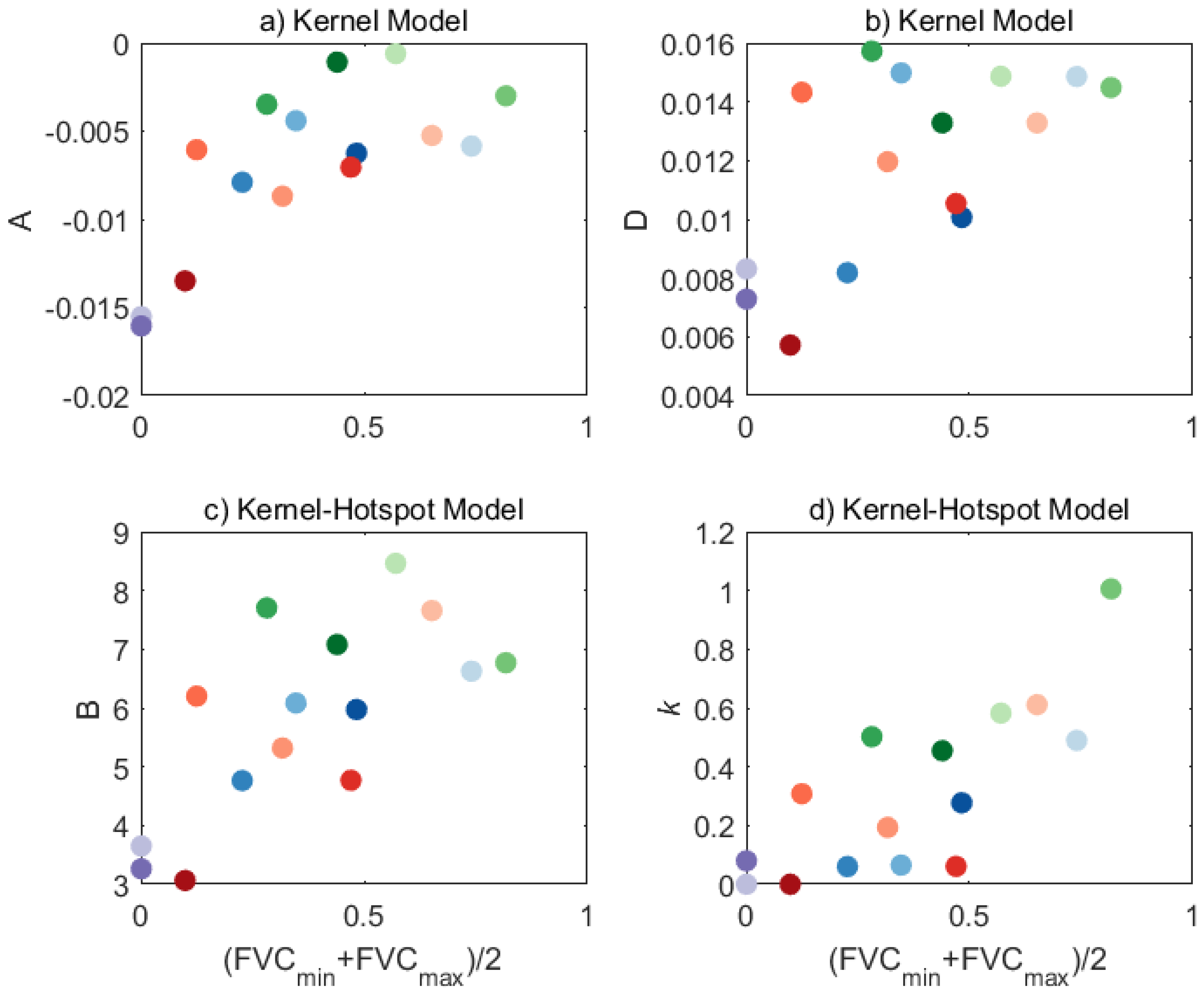
The parametric models were fitted to the LST datasets of each cluster of pixels, and Figure 3 shows the respective obtained parameters. It may be noted that the emissivity kernel parameter, A, presents only negative values. This indicated a decrease of the LST with VZA, which is consistent with a decrease of emissivity with view angle. Emissivity is known to decrease with VZA for homogenous surfaces like bare ground (e.g., [28]) but this variation is expected to be negligible for rough surfaces like those that are vegetated [29,30,31]. The highest absolute values of A were obtained for clusters with low FVC and there was a tendency for absolute values of A to decrease with increasing FVC (Figure 4). The impact of emissivity anisotropy on LST was likely to be related with the fraction of bare ground that is within the satellite FOV, and therefore it is expected that this impact would be larger for lower vegetation cover.
The fitting of the solar kernel led to positive values of parameter D (Figure 3a). Taking into account Equation (3) and noting that is maximum at the hotspot (i.e., when the sun is effectively positioned behind the sensor), a positive value of D indicated that LST tended to increase relative to nadir as the satellite approached the hot-spot configuration and decreased for the remaining sun-sensor relative positions. For heterogeneous surfaces (e.g., tree/shrub covered), the LST anisotropy was mostly related to shadowing effects and, therefore, this effect was expected to be more relevant over moderately vegetated surfaces. Moreover, the higher D values were obtained for intermediate FVC values, although the relation to FVC was not as clear as in the case of A (see Figure 4a,b). Other factors are also relevant in this case, e.g., typical temperature contrasts, height and volume of the vegetation objects, and surface topography [8,17,20,32,33].
The calibration of the Kernel-Hotspot model also led to positive values of parameter B (Figure 3b). Given the dependence of Equation (5) on parameter , a positive B indicated that the hot-spot configuration was associated with LST values that were warmer than those that would be measured from the nadir configuration. As in the case of the solar kernel parameter, D, the higher values of B were associated to intermediate values of FVC, although this quantity did not translate the full variability of B (Figure 4c). The fit also resulted in positive values of k for the majority of the clusters (Figure 3b). According to [34], this parameter was closely linked to the density of vegetation in the reflectance model, and the study by [15], based essentially on simulated data showed a linear dependence of k with the percentage of tree cover. We found that k tends to increase with the average FVC (Figure 4d), in agreement with these studies. Near-zero values of k occurred for very low values of FVC, when shadowing effects were very weak or absent. Although the emissivity effect was here accounted for, values of B were still significant for very low FVC, which suggests that geometric effects that are not related to emissivity may still exist, or that the emissivity kernel is not able to fully represent the LST anisotropy.
4.3. Assessment of Models’ Performance
4.3.1. Performance over the Calibration Database
The ability of the parametric models to correct for angular effects is first analyzed using the LST matchup dataset build for the calibration, which provides a better spatial coverage, and a higher number of matchups. It should be noted that although the same data are used here to both calibrate and assess the models’ performance, the calibration is nevertheless performed over clusters of pixels while the performance is assessed on a pixel-by-pixel basis.
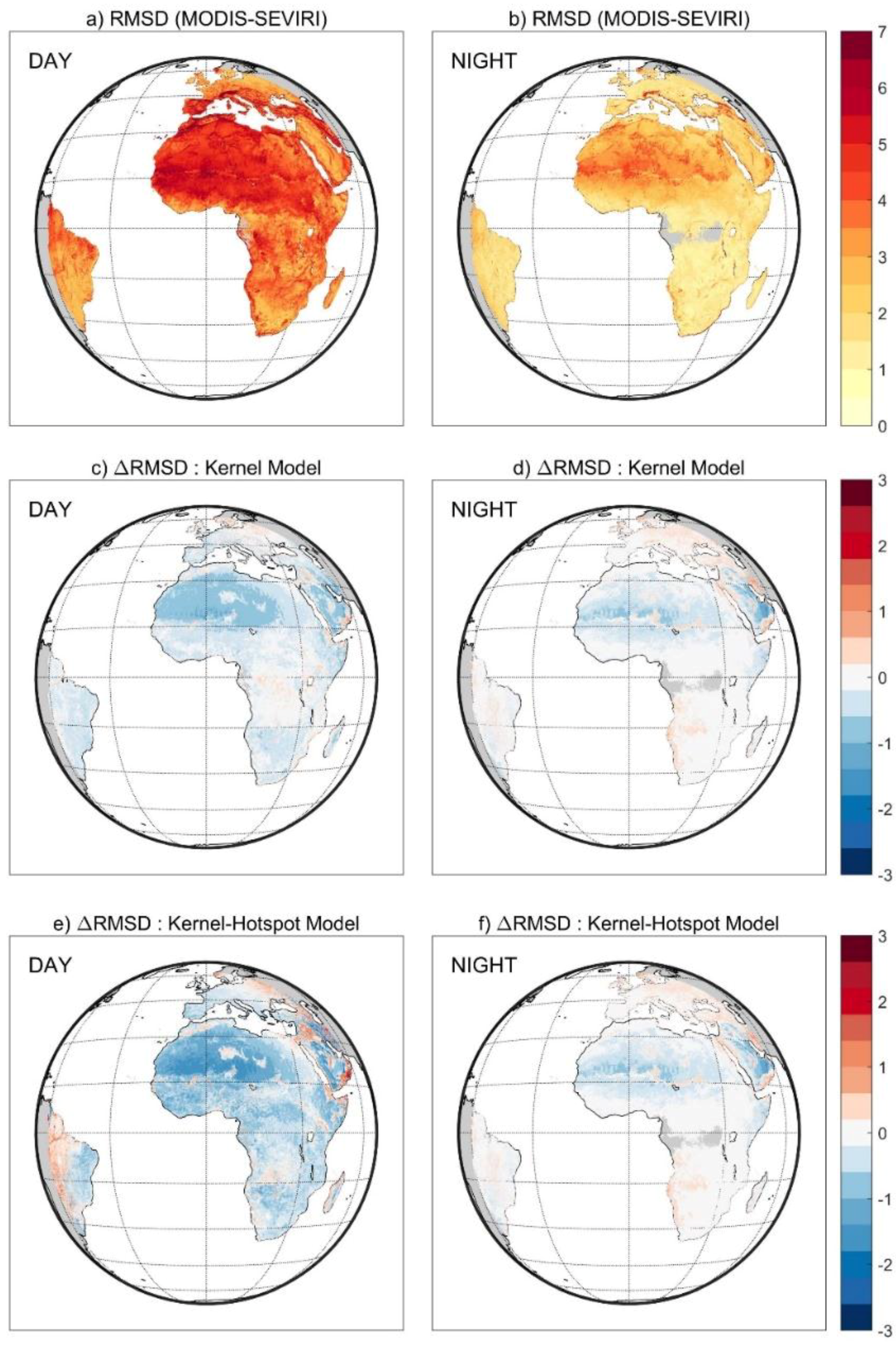
The performance of each model takes into account its capability to simulate the differences in LST fields estimated from different sensors (and different viewing geometries) collocated in space and time. As such, we first use the model to correct one of the sensors’ LST to the viewing configuration of the other and then comparing LST differences before and after that correction. The angular correction should lead to closer values of LST between the sensors [17], and therefore to a reduction of the respective root mean square difference (RMSD). It is worth noting that the models were here used to correct SEVIRI LST to the viewing geometry of MODIS. Figure 5 presents the spatial distribution of RMSD between MODIS and SEVIRI LST, and the impact of the angular corrections as given by each model, showing the change in the RMSD of LST values (i.e., (RMSD after angular correction)–(original RMSD)). Since the angular adjustment was performed on data that were previously bias-corrected, the role of both corrections was assessed separately by means of a histogram of RMSD change (Figure 6). The performance of the models with respect to the Kernel model calibrated on a pixel-by-pixel basis (as done in [17]) is also analyzed in the histogram of Figure 6.
During the daytime, the Kernel model led to an overall decrease of the RMSD between the sensors, with only a small percentage of the pixels (5.7%) presenting an increase of the LST differences. LST RMSD changes (ΔRMSD) are as high as −1.6 K (percentile 0.1%) and −0.5 K on average. For the Kernel-Hotspot model the angular correction also leads mostly to a decrease of the RMSD, with a slightly lower percentage of the pixels (3.2%) presenting an increase. The average ΔRMSD given by this model is −1.1 K, and corrections are as high as −5.5 K (percentile 0.1%).
During night-time, there was also a general decrease in the LST RMSD when the Kernel model is used to correct angular effects. As expected, corrections were lower than during daytime, leading to an average ΔRMSD of −0.2 K, with values up to −1.4 K (percentile 0.1%). In this case, a larger percentage of pixels (15.6%) showed an increase in RMSD, but for most of these (84.2%), the increase is below 0.2 K.
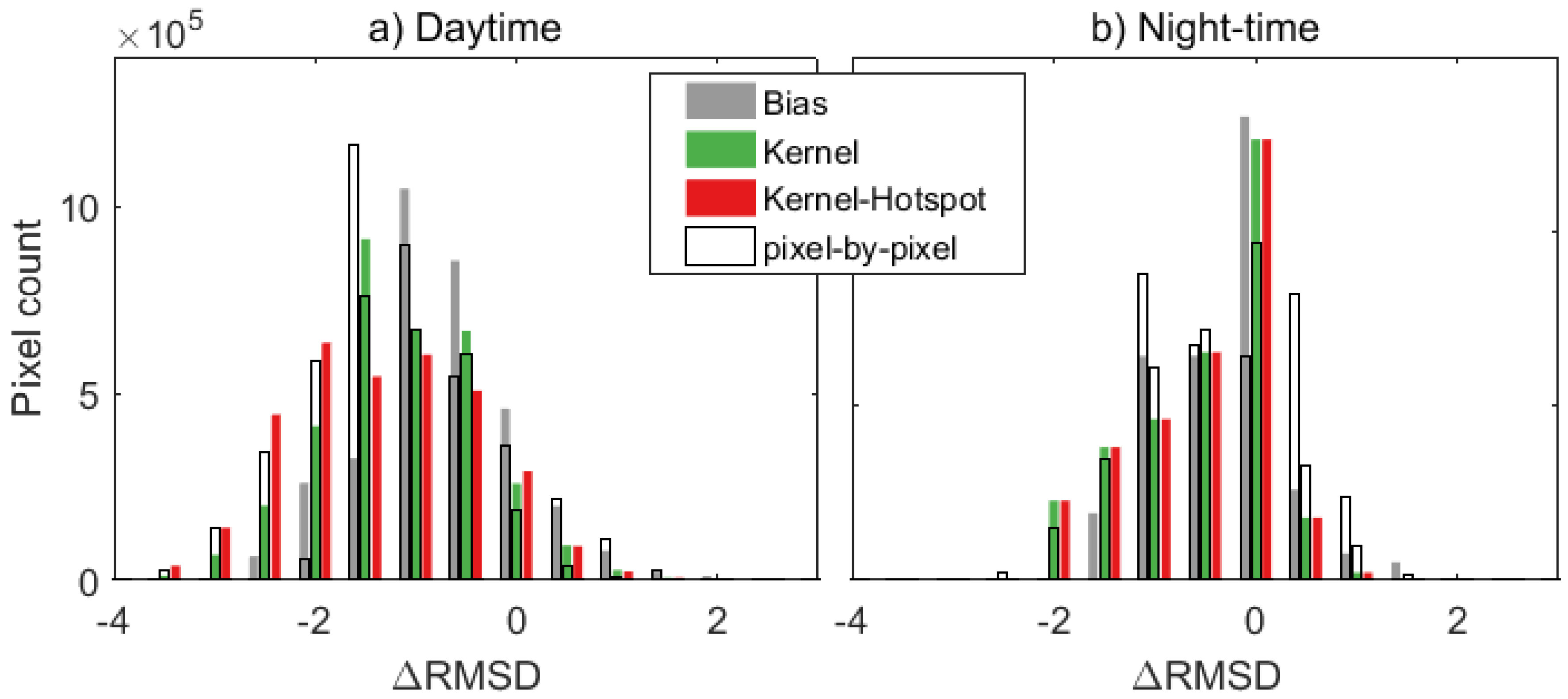
It may be noted that all models led to a shift of the distribution of ΔRMSD towards lower values (Figure 6) and that such displacement is higher for the Kernel-Hotspot model. This indicates that the Kernel-Hotspot model present an overall better performance than the Kernel model. There was also a larger shift of the RMSD distribution of the pixel-based Kernel model than the cluster-based one; however, both were outperformed by the combined Kernel-Hotspot, which was larger. This suggests a better performance of the Kernel-Hotspot model than that of the Kernel model for both the cluster-based and the pixel-based approaches.
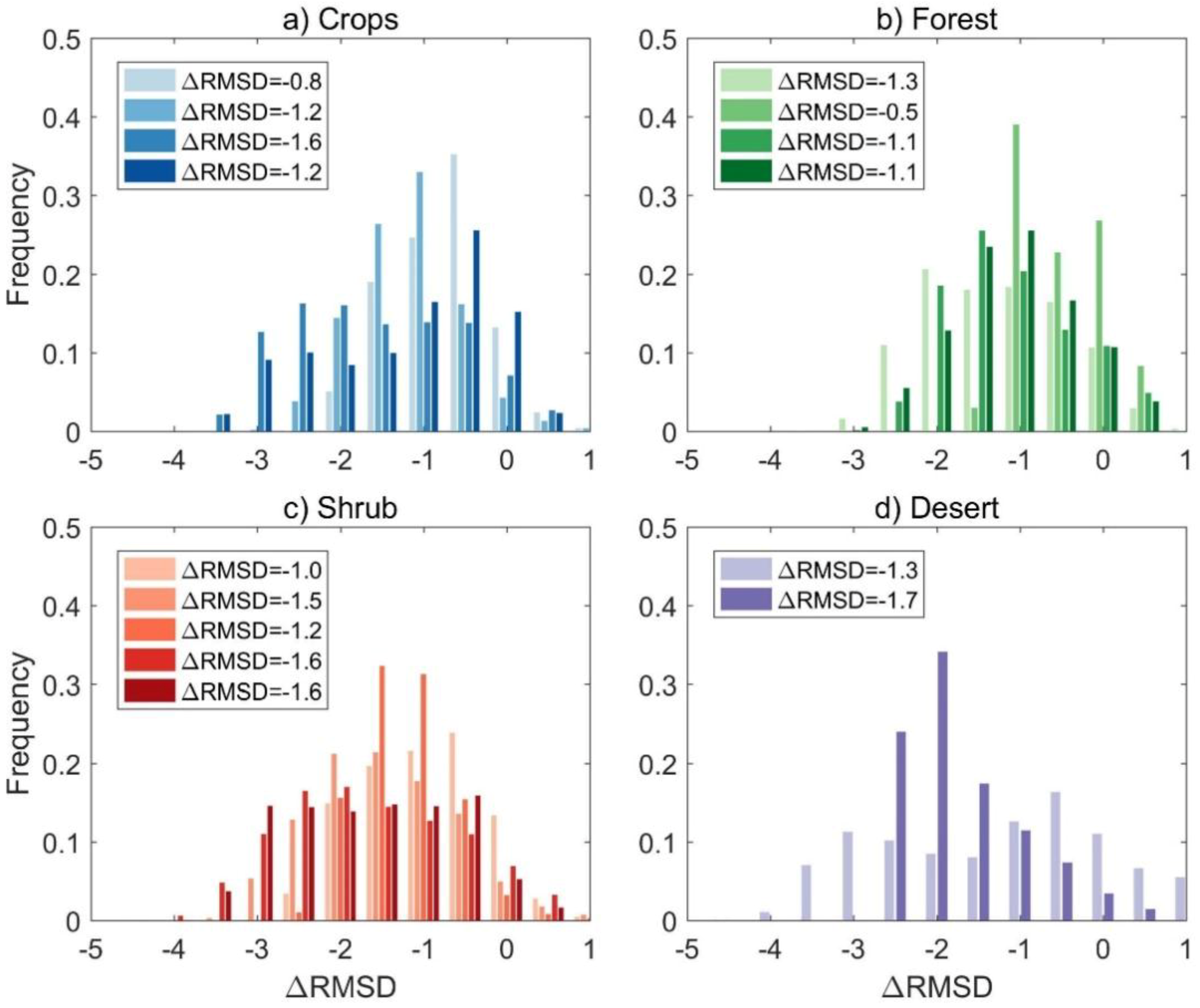
The performance of the Kernel-Hotspot model was further analyzed for each cluster separately (Figure 7). During daytime, the highest angular corrections were generally found for forest and shrubland, namely the shrub clusters associated to savanna-like vegetation cover (e.g., in central Africa and the Iberian Peninsula). These land cover types were particularly prone to shadowing effects [8,19,35]. The desert areas also presented large corrections, being more susceptible to anisotropic effects associated to the emissivity [29,31]. The higher percentages of positive values of ΔRMSD are found for the second cluster of the forest group (Figure 7b), and for the first cluster of the desert group (Figure 7d). For the forest cluster, the respective k parameter was much larger than the remaining clusters (Figure 3b), which might indicate problems in the calibration. This cluster was associated to equatorial forests (Figure 1) where there is generally higher cloud coverage. This not only strongly limited the amount of available matchups but could also be associated to a higher frequency of cloud contamination of the LST estimates. The desert cluster associated to high elevations (i.e., the cluster of non-vegetated elevated regions) corresponded to areas with high topography heterogeneity (Figure 2). These areas were particularly challenging, since the high heterogeneity enhances geo-referencing errors. Also, slope and orientation of the mountain ridges could introduce shadowing effects that are not fully accounted for by either the Kernel or Kernel-Hotspot models [17].
4.3.2. Performance with an Independent Dataset
The performance of the parametric models was then investigated using an independent dataset of collocated LST over selected areas. Figure 8 shows the RMSD between MODIS and each GEO of the GT_MDB, and the impact of the angular correction on the RMSD as performed by the Kernel-Hotspot model (ΔRMSD).
In the case of the GT_MDB dataset, GEOs data are only processed on an hourly basis, which strongly limits the number of matchups with MODIS. For that reason, it is possible to distinguish marked patterns in the RMSD maps (Figure 8, first and third columns) associated to the predominance of MODIS observations performed in the center or edge of MODIS’ scan, with the highest RMSD values being associated to higher VZA values. For the same reason, the angular corrections present similar patterns (Figure 8, second and fourth columns).
Values of ΔRMSD were within the range of values obtained in the previous section, and there was a consistency between selected regions. This indicates that, despite having been calibrated only with SEVIRI and MODIS LST, the model shows a similar performance when applied to different sensors, as well as to SEVIRI–MODIS matchup gathered over a different period than that used for calibration purposes.
The highest daytime corrections were observed over the savanna areas of Iberia (IBE), Northwest Africa (WAF), and Australia (AUS), and the highest night-time corrections occurred in the Saharadesert (WAF) and Australia (AUS), in agreement with the results discussed in the previous section. The night-time corrections in the Namib desert were reduced, as were the RMSD values, likely due to the lower VZAs associated to this area.
There was a slight increase of the RMSD in some areas that seemed to be associated to low VZAs of MODIS. This was likely due to inconsistencies between the LST products in the calibration database, i.e., LST differences between the two sensors at low VZAs were larger than what would be expected from geometric effects.
4.4. Simulation of the Angular Corrections on LST
The Kernel and Kernel-Hotspot models calibrated per cluster may finally be used to quantify the expected angular effects on LST retrieved by any given sensor. Examples of obtained values for differences T-T0 (ΔLST) when using the Kernel and Kernel-hotspot models are shown in Figure 9 and Figure 10 for SEVIRI/MSG based observations at four different observation time-slots for the 15 July 2017 (chosen arbitrarily).
During night-time (00:00 UTC; Figure 9a,c,e), the angular corrections should be solely due to emissivity effects, which are simulated by the emissivity kernel. As such, night-time corrections were the same for the Kernel and Kernel-Hotspot models. The largest corrections were observed over the desert areas over the eastern-most part of the disk, encompassing the Arabian Peninsula and Asian regions surrounding the Caspian Sea.
The angular corrections provided by the by the Kernel model are particularly conspicuous at 12:00 UTC (Figure 9d), showing high discrepancies when compared to the Kernel-Hotspot. At this time of the day over Europe, SEVIRI was particularly prone to hotspot effects, which led to high negative corrections to nadir. The corrections provided by the Kernel-Hotspot model over the Iberian Peninsula were in agreement with those found with the Geometric model for Évora by [17]. The Kernel model, however, showed a very contrasting behavior presenting positive corrections over most Europe. This seems to be related to limitations in the simulation of the hotspot effect by the Kernel model, as previously pointed out by [36] and [15].
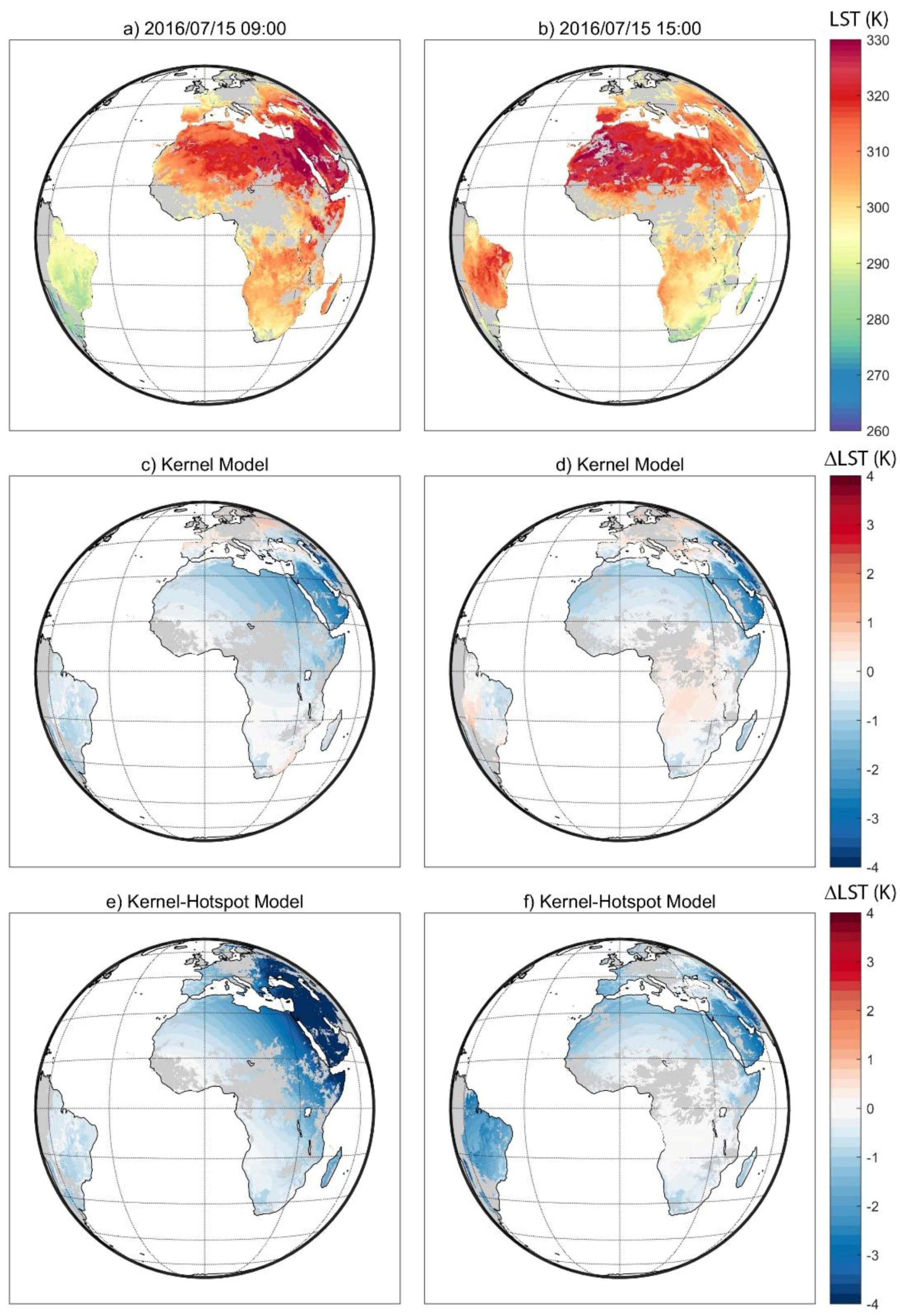
Examples of the expected angular corrections are also shown for mid-morning (09:00 coordinated universal time (UTC); Figure 10a,c,e) and mid-afternoon (15:00 UTC; Figure 10b,d,f). As expected, corrections at these observation times seemed to be mostly controlled by the view angle. Close-to-hotspot geometries occurred over the western and eastern parts of the disk for 09 and 15:00 UTC, respectively, which resulted in enhanced corrections over those regions (Figure 10e,f, respectively). Corrections were particularly high over the eastern part of the disk (Figure 10e). The angular corrections also depended non-linearly on the LST values, and therefore tended to be higher for daytime, even for desert areas where shadowing effects were reduced. Nevertheless, values of B over desert clusters were still significant, despite the emissivity effect being accounted for by the emissivity kernel. As such, the hotspot component will also enhance daytime corrections over desert areas, partly due to the very high LST values observed there (Figure 10e).
It should be noted that the values of B derived over the desert areas could be associated to discrepancies in the LST products not related to viewing geometries. This indicates that the Kernel-Hotspot model was particularly sensitive to the LST datasets used in the calibration. The calibration dataset should ideally correspond to LST matchups derived with the same algorithm and using inter-calibrated top-of-atmosphere brightness temperatures to avoid overfitting of the model.
5. Discussion
The first step in the preparation of the LST database for the calibration of the parametric models is the removal of any systematic differences between MODIS and SEVIRI LSTs that are not related to the viewing geometry. These include differences in input data, atmospheric correction, and algorithm, amongst others. The residuals of the regressions used for this bias correction (Table 1) are still significant, with RMSD ranging between 0.94 and 1.22 K, which indicates that some of these unwanted differences may still impact the quality of the calibration.
The distributions of the models’ parameters reflect the main characteristics of the clusters’ landscape. Values of A (emissivity kernel) are always negative and show an inverse relation with the density of vegetation, whereas parameters D (Kernel model) and k and B (Kernel-Hotspot) generally present an increase with increasing fraction of vegetation. This is in agreement with the relationships previously found between these models and vegetation indicators [15,17].
The obtained models’ coefficients lead to an overall reduction of the RMSD between the two LST datasets, with corrections as high as 1.6 K and 5.5 K for the Kernel and Kernel-Hotspot models, respectively. The higher corrections of the Kernel-Hotspot model indicate a better performance of this model in simulating the angular dependence of LST, in accordance with previous studies [15,37]. However, some areas still show an increase in the RMSD (Figure 5). This increase could be related to regions of higher discrepancies between MODIS and SEVIRI that are not accounted for by the bias corrections (e.g., the mountainous areas of Africa and of the Arabian Peninsula). Some of these regions are located at the edge of SEVIRI disk, where there is both a degradation of SEVIRI’s resolution and uncertainties of the LST product are expected to be higher.
However, the Kernel-Hotspot seems to be particularly sensitive to the calibration database. This is to be expected as this model is able to provide larger corrections than the Kernel method. As a result, LST discrepancies between the LST products, which are not associated with the viewing geometry and that were not fully accounted for in the bias correction, often lead to overfitting of the model. Consequently, angular corrections may be overestimated by this model. This effect is seen in Figure 5, where regions of positive ΔRMSE have higher amplitude in the case of the Kernel-Hotspot (Figure 5e) than of the Kernel model (Figure 5c). As such, to avoid overfitting problems, the model should be fitted to LST data that were previously calibrated and processed using the same or very similar algorithms applied preferably to intercalibrated radiances.
6. Conclusions
The correction of directional effects on satellite-retrieved LST is of high relevance for a proper interpretation of spatial and temporal features contained in LST fields. Previous studies have found that LST differences between products induced by geometric effects may be as high as 15 K [8,37,38].
The present study proposes a methodology to simulate directional effects of LST products, using parametric models calibrated with satellite observations. The main limitation found in the calibration of such models using satellite-retrieved LST matchups seems to be associated with the high impact of LST discrepancies among different satellite products, which are not related to the viewing geometry [17]. To partially overcome such problems, we propose a calibration procedure where a cluster approach is used to aggregate pixels with similar landscape characteristics, allowing an effective reduction of overfitting to local biases, and a better sampling of view and illumination angles.
It is shown that the use of the models calibrated per cluster to correct for angular effects reduces the differences between the two products. Decreases in RMSD are found to be larger for the Kernel-Hotspot model than for the Kernel model. This higher efficiency of the Kernel-Hotspot model in correcting angular effects is in agreement with the assessment shown in [15]. Furthermore, it is shown that the models’ coefficients calibrated over a limited area, but using a surface classification, are appropriate for use in other regions of the globe with the same classification, even when using different sensors.
This study shows that collocated satellite observations may be used to calibrate parametric models that in turn allows an effective representation of directional effects on LST. Both methods assessed here can be easily be extended to other sensors, and the simplicity of the approach makes it particularly appropriate to be used in an operational context. This methodology is used within the framework of the European Space agency (ESA) Data User Element (DUE) GlobTemperature project. Information on angular effects on LST is provided in a data layer in the Merged LST product that consists in an estimate of LST difference from the nadir to the satellite view.
Within the framework of the LSA-SAF, a similar methodology is being assessed to an additional data layer the operational SEVIRI/Meteosat LST product generated every 15 min. As in the case above, this layer will consist of an estimate of the LST difference from the nadir to the SEVIRI view, thus providing the user with information on the expected deviation of the actual retrieval due to angular effects, on a pixel-by-pixel basis.
Author Contributions
Investigation, S.L.E.; Methodology, S.L.E., I.F.T., C.C.D. and A.C.P.; Supervision, I.F.T. and C.C.D.; Validation, S.L.E.; Writing—original draft, S.L.E.; Writing—review & editing, I.F.T. and C.C.D.
Funding
Research by Sofia L. Ermida was supported by the Portuguese Science Foundation (FCT) through the PhD grant SFRH/BD/96466/2013.
Acknowledgments
This work was performed within the framework of ESA DUE GlobTemperature (http://www.globtemperature.info/) and LSA SAF (http://landsaf.ipma.pt) projects. The SEVIRI/MSG LST data were generated by the LSA SAF project funded by EUMETSAT. The MODIS LST data (MOD/MYD11) were retrieved from the online Reverb/ECHO, courtesy of the NASA EOSDIS Land Processes Distributed Active Archive Center (LP DAAC), USGS/Earth Resources Observation and Science (EROS) Center, Sioux Falls, South Dakota (http://reverb.echo.nasa.gov). The GlobTemperature matchup database (GT_MDB) data was obtained through the GlobTemperature portal (http://data.globtemperature.info/).
Conflicts of Interest
The authors declare no conflict of interest. The funders had no role in the design of the study; in the collection, analyses, or interpretation of data; in the writing of the manuscript, and in the decision to publish the results.
References
- Norman, J.M.; Becker, F. Terminology in thermal infrared remote sensing of natural surfaces. Agric. For. Meteorol. 1995, 77, 153–166. [Google Scholar] [CrossRef]
- Kerr, Y.H.; Lagouarde, J.P.; Nerry, F.; Ottlé, C. Land surface temperature retrieval techniques and applications. In Thermal Remote Sensing in Land Surface Processes; CRC Press: Boston, MA, USA, 2004; pp. 33–109. [Google Scholar]
- Lagouarde, J.P.; Ballans, H.; Moreau, P.; Guyon, D.; Coraboeuf, D. Experimental study of brightness surface temperature angular variations of maritime pine (Pinus pinaster) stands. Remote Sens. Environ. 2000, 72, 17–34. [Google Scholar] [CrossRef]
- Pinheiro, A.C.T.; Privette, J.L.; Mahoney, R.; Tucker, C.J. Directional effects in a daily AVHRR land surface temperature dataset over Africa. IEEE Trans. Geosci. Remote Sens. 2004, 42, 1941–1954. [Google Scholar] [CrossRef]
- Pinheiro, A.C.T.; Privette, J.L.; Guillevic, P. Modeling the observed angular anisotropy of land surface temperature in a Savanna. IEEE Trans. Geosci. Remote Sens. 2006, 44, 1036–1047. [Google Scholar] [CrossRef]
- Barroso, C.; Trigo, I.F.; Olesen, F.; DaCamara, C.; Queluz, M.P. Intercalibration of NOAA and Meteosat window channel brightness temperatures. Int. J. Remote Sens. 2005, 26, 3717–3733. [Google Scholar] [CrossRef]
- Trigo, I.F.; Monteiro, I.T.; Olesen, F.; Kabsch, E. An assessment of remotely sensed land surface temperature. J. Geophys. Res. 2008, 113, 1–12. [Google Scholar] [CrossRef]
- Ermida, S.L.; Trigo, I.F.; Dacamara, C.C.; Göttsche, F.M.; Olesen, F.S.; Hulley, G. Validation of remotely sensed surface temperature over an oak woodland landscape—The problem of viewing and illumination geometries. Remote Sens. Environ. 2014, 148, 16–27. [Google Scholar] [CrossRef]
- Duffour, C.; Lagouarde, J.P.; Olioso, A.; Demarty, J.; Roujean, J.L. Driving factors of the directional variability of thermal infrared signal in temperate regions. Remote Sens. Environ. 2016, 177. [Google Scholar] [CrossRef]
- Duffour, C.; Olioso, A.; Demarty, J.; Van der Tol, C.; Lagouarde, J.P. An evaluation of SCOPE: A tool to simulate the directional anisotropy of satellite-measured surface temperatures. Remote Sens. Environ. 2015, 158, 362–375. [Google Scholar] [CrossRef]
- Caselles, V.; Sobrino, J.; Coll, C. A physical model for interpreting the land surface temperature obtained by remote sensors over incomplete canopies. Remote Sens. Environ. 1992, 39, 203–211. [Google Scholar] [CrossRef]
- Sobrino, J.; Caselles, V. Thermal infrared radiance model for interpreting the directional radiometric temperature of a vegetative surface. Remote Sens. Environ. 1990, 33, 193–199. [Google Scholar] [CrossRef]
- Smith, J.A.; Goltz, S.M. A thermal exitance and energy balance model for forest canopies. IEEE Trans. Geosci. Remote Sens. 1994, 32, 1060–1066. [Google Scholar] [CrossRef]
- Li, X.; Strahler, A.H. Geometric-optical bidirectional reflectance modeling of the discrete crown vegetation canopy: Effect of crown shape and mutual shadowing. Trans. Geosci. Remote Sens. 1992, 30, 276–292. [Google Scholar] [CrossRef]
- Ermida, S.L.; Trigo, I.F.; DaCamara, C.C.; Roujean, J.-L. Assessing the potential of parametric models to correct directional effects on local to global remotely sensed LST. Remote Sens. Environ. 2018, 209. [Google Scholar] [CrossRef]
- Vinnikov, K.Y.; Yu, Y.; Goldberg, M.D.; Tarpley, D.; Romanov, P.; Laszlo, I.; Chen, M. Angular anisotropy of satellite observations of land surface temperature. Geophys. Res. Lett. 2012, 39, L23802. [Google Scholar] [CrossRef]
- Ermida, S.L.; DaCamara, C.C.; Trigo, I.F.; Pires, A.C.; Ghent, D.; Remedios, J. Modelling directional effects on remotely sensed land surface temperature. Remote Sens. Environ. 2017, 190. [Google Scholar] [CrossRef]
- Lagouarde, J.P.; Irvine, M. Directional anisotropy in thermal infrared measurements over Toulouse city centre during the CAPITOUL measurement campaigns: First results. Meteorol. Atmos. Phys. 2008, 102, 173–185. [Google Scholar] [CrossRef]
- Rasmussen, M.O.; Pinheiro, A.C.; Proud, S.R.; Sandholt, I. Modeling angular dependences in land surface temperatures from the SEVIRI instrument onboard the geostationary meteosat second generation satellites. IEEE Trans. Geosci. Remote Sens. 2010, 48, 3123–3133. [Google Scholar] [CrossRef]
- Lagouarde, J.P.; Kerr, Y.H.; Brunet, Y. An experimental study of angular effects on surface temperature for various plant canopies and bare soils. Agric. For. Meteorol. 1995, 77, 167–190. [Google Scholar] [CrossRef]
- Trigo, I.F.; Dacamara, C.C.; Viterbo, P.; Roujean, J.-L.; Olesen, F.; Barroso, C.; Camacho-de-Coca, F.; Carrer, D.; Freitas, S.C.; García-Haro, J.; et al. The satellite application facility for land surface analysis. Int. J. Remote Sens. 2011, 32, 2725–2744. [Google Scholar] [CrossRef]
- Wan, Z.; Li, Z.-L. Radiance-based validation of the V5 MODIS land-surface temperature product. Int. J. Remote Sens. 2008, 29, 5373–5395. [Google Scholar] [CrossRef]
- Wan, Z.; Dozier, J. A generalized split-window algorithm for retrieving land-surface temperature from space. IEEE Trans. Geosci. Remote Sens. 1996, 34, 892–905. [Google Scholar]
- Freitas, S.C.; Trigo, I.F.; Bioucas-Dias, J.M.; Göttsche, F. Quantifying the uncertainty of land surface temperature retrievals from SEVIRI/Meteosat. IEEE Trans. Geosci. Remote Sens. 2010, 48, 523–534. [Google Scholar] [CrossRef]
- Meeus, J. Astronomical Algorithms, 2nd ed.; Willmann-Bell, Incorporated: Richmond, VA, USA, 1991; ISBN 0943396352. [Google Scholar]
- Lagarias, J.C.; Reeds, J.A.; Wright, M.H.; Wright, P.E. Convergence properties of the nelder-mead simplex method in low dimensions. SIAM J. Optim. 1998, 9, 112–147. [Google Scholar] [CrossRef]
- Seber, G.A. Multivariate Observations; Hoboken, N., Ed.; John Wiley & Sons: Hoboken, NJ, USA, 1984. [Google Scholar]
- McAtee, B.K.; Prata, A.J.; Lynch, M.J.; McAtee, B.K.; Prata, A.J.; Lynch, M.J. The angular behavior of emitted thermal infrared radiation (8–12 μm) at a semiarid site. J. Appl. Meteorol. 2003, 42, 1060–1071. [Google Scholar] [CrossRef]
- Labed, J.; Stoll, M.P. Angular variation of land surface spectral emissivity in the thermal infrared: Laboratory investigations on bare soils. Int. J. Remote Sens. 1991, 12, 2299–2310. [Google Scholar] [CrossRef]
- Ren, H.; Yan, G.; Chen, L.; Li, Z. Angular effect of MODIS emissivity products and its application to the split-window algorithm. ISPRS J. Photogramm. Remote Sens. 2011, 66, 498–507. [Google Scholar] [CrossRef]
- Sobrino, J.A.; Cuenca, J. Angular variation of thermal infrared emissivity for some natural surfaces from experimental measurements. Appl. Opt. 1999, 38, 3931–3936. [Google Scholar] [CrossRef] [PubMed]
- Li, X.; Strahler, A. Geometric-optical bidirectional reflectance modeling of a conifer forest canopy. Trans. Geosci. Remote Sens. 1986, GE-24, 906–919. [Google Scholar] [CrossRef]
- Franklin, J.; Strahler, A.H. Invertible canopy reflectance modeling of vegetation structure in semiarid woodland. IEEE Trans. Geosci. Remote Sens. 1988, 26, 809–825. [Google Scholar] [CrossRef]
- Roujean, J.-L. A parametric hot spot model for optical remote sensing application. Remote Sens. Environ. 2000, 71, 197–206. [Google Scholar] [CrossRef]
- Guillevic, P.C.; Bork-Unkelbach, A.; Göttsche, F.M.; Hulley, G.; Gastellu-Etchegorry, J.-P.; Olesen, F.S.; Privette, J.L. Directional viewing effects on satellite land surface temperature products over sparse vegetation canopies—A multisensor analysis. IEEE Geosci. Remote Sens. Lett. 2013, 10, 1464–1468. [Google Scholar] [CrossRef]
- Duffour, C.; Lagouarde, J.-P.; Roujean, J.-L. A two parameter model to simulate thermal infrared directional effects for remote sensing applications. Remote Sens. Environ. 2016, 186, 250–261. [Google Scholar] [CrossRef]
- Rasmussen, M.O.; Göttsche, F.; Olesen, F.; Sandholt, I. Directional effects on land surface temperature estimation from meteosat second generation for savanna landscapes. IEEE Trans. Geosci. Remote Sens. 2011, 49, 4458–4468. [Google Scholar] [CrossRef]
- Lagouarde, J.P.; Dayau, S.; Moreau, P.; Guyon, D. Directional anisotropy of brightness surface temperature over vineyards: Case study over the Medoc Region (SW France). IEEE Geosci. Remote Sens. Lett. 2014, 11, 574–578. [Google Scholar] [CrossRef]
Figure 1.
Spatial distribution of the cluster-based surface classification. The rectangles indicate the areas used in the model evaluation with the GT_MDB.
Figure 1.
Spatial distribution of the cluster-based surface classification. The rectangles indicate the areas used in the model evaluation with the GT_MDB.

Figure 2.
Cluster centroids of the surface classification in terms of their annual maximum and minimum fraction of vegetation cover (FVC). The size of the circles represents the clusters mean elevation (see legend) and colors correspond to the color bar of Figure 1.
Figure 2.
Cluster centroids of the surface classification in terms of their annual maximum and minimum fraction of vegetation cover (FVC). The size of the circles represents the clusters mean elevation (see legend) and colors correspond to the color bar of Figure 1.
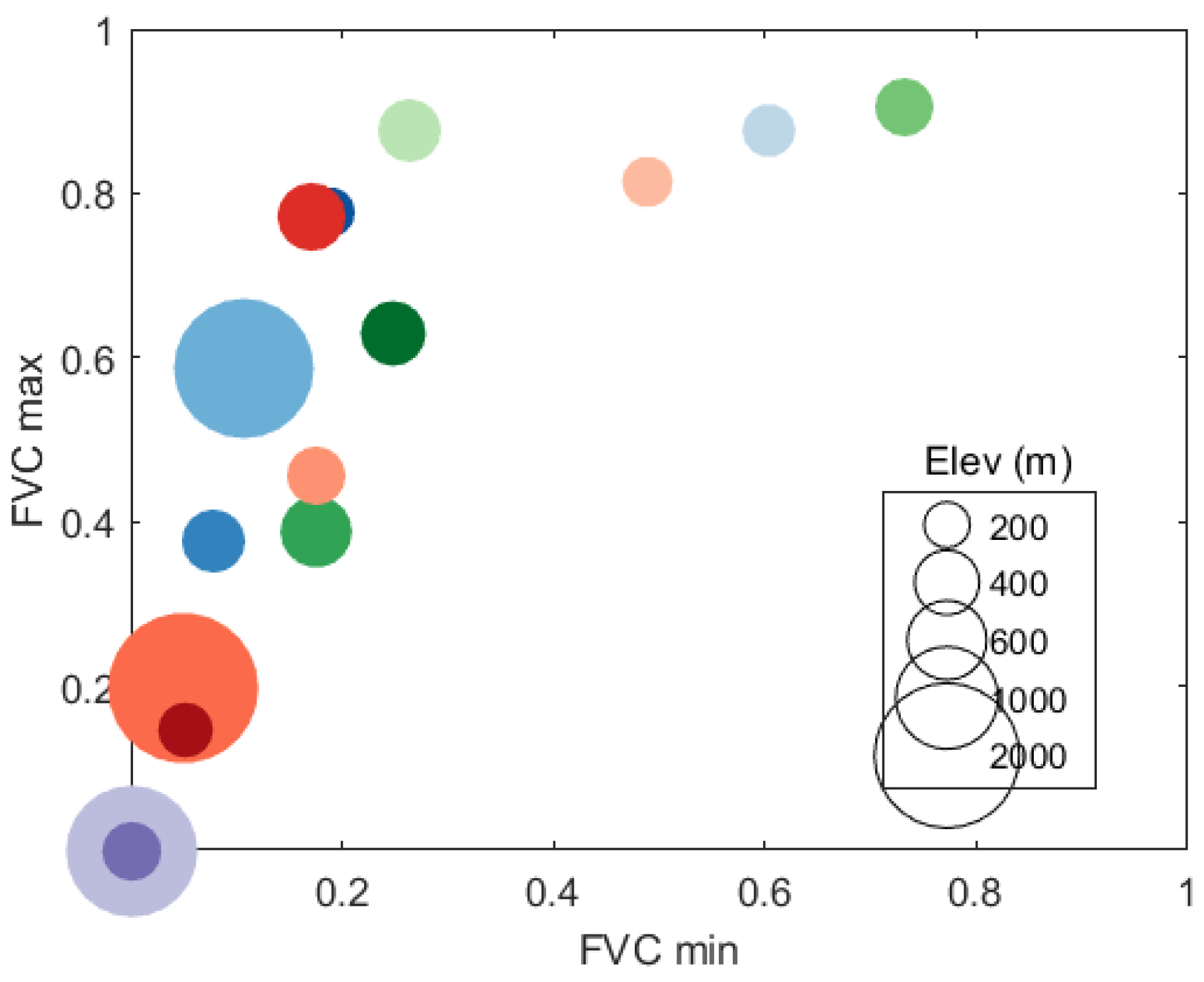
Figure 3.
Coefficients of the (a) Kernel and (b) Kernel-Hotspot models. Values of parameter A derived for the Kernel model are kept the same in the Kernel-Hotspot model (a). Colors indicate the different clusters of pixels and correspond to the color bar of Figure 1.
Figure 3.
Coefficients of the (a) Kernel and (b) Kernel-Hotspot models. Values of parameter A derived for the Kernel model are kept the same in the Kernel-Hotspot model (a). Colors indicate the different clusters of pixels and correspond to the color bar of Figure 1.
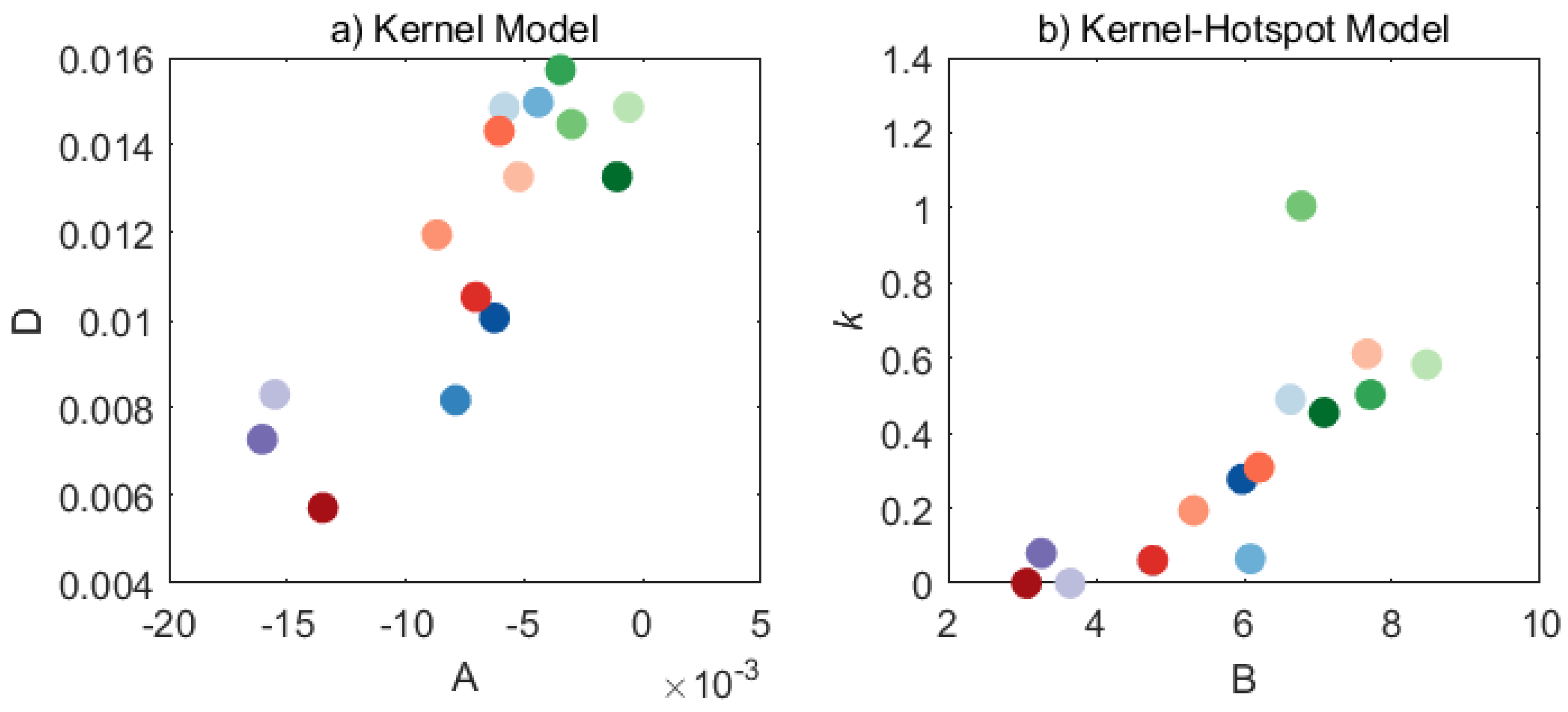
Figure 4.
Parameters of the Kernel (a,b) and Kernel-Hotspot (c,d) models as function of the average FVC of the cluster. Colors indicate the different clusters of pixels and correspond to the color bar of Figure 1.
Figure 4.
Parameters of the Kernel (a,b) and Kernel-Hotspot (c,d) models as function of the average FVC of the cluster. Colors indicate the different clusters of pixels and correspond to the color bar of Figure 1.

Figure 5.
Spatial distribution of Root Mean Square Differences (RMSD) between SEVIRI and MODIS (K) without angular correction (a,b) and impact of LST angular correction on RMSD (in K; as (RMSD after angular correction)–(RMSD without correction)), as given by the Kernel model (c,d) and the Kernel-Hotspot model (e,f) when applied to data used in the calibration. The results are shown for daytime (left panels) and night-time (right panels) scenes, respectively.

Figure 6.
Histograms of variation of the root mean square differences (ΔRMSD) between SEVIRI and MODIS (in K) after applying the bias correction (grey) and after applying the angular correction with the Kernel model (green) and the Kernel-Hotspot model (red), for (a) daytime and (b) night-time only observations. The open bars are the respective values for the pixel-based model.

Figure 7.
Distributions of the variation of the daytime root mean square differences (ΔRMSD) between SEVIRI and MODIS (in K) after applying the angular correction of the Kernel-Hotspot model, for each cluster within each land cover type: (a) crops, (b) forest, (c) shrub, and (d) desert. Colors correspond to the color bar of Figure 1. The legend shows the average ΔRMSD for each cluster.

Figure 8.
Spatial distribution of Root Mean Square Differences (RMSD; 1st and 3rd columns; in K) between MODIS and each geostationary sensor part of the GT_MDB, as well as the impact of LST angular correction on the RMSD (in K; as (RMSD after angular correction)–(RMSD without correction)), as given by the Kernel-Hotspot model (second and fourth columns). The geostationary satellite considered varies with area, namely: SEVIRI (SEV) over the Iberian Peninsula (IBE), West Africa (WAF) and the Namib desert (NAM); GOES (GOE) over the Southern Great Plains (SGP); and MTSAT-2 (MTS), and Himawari (HMW) over Australia (AUS).
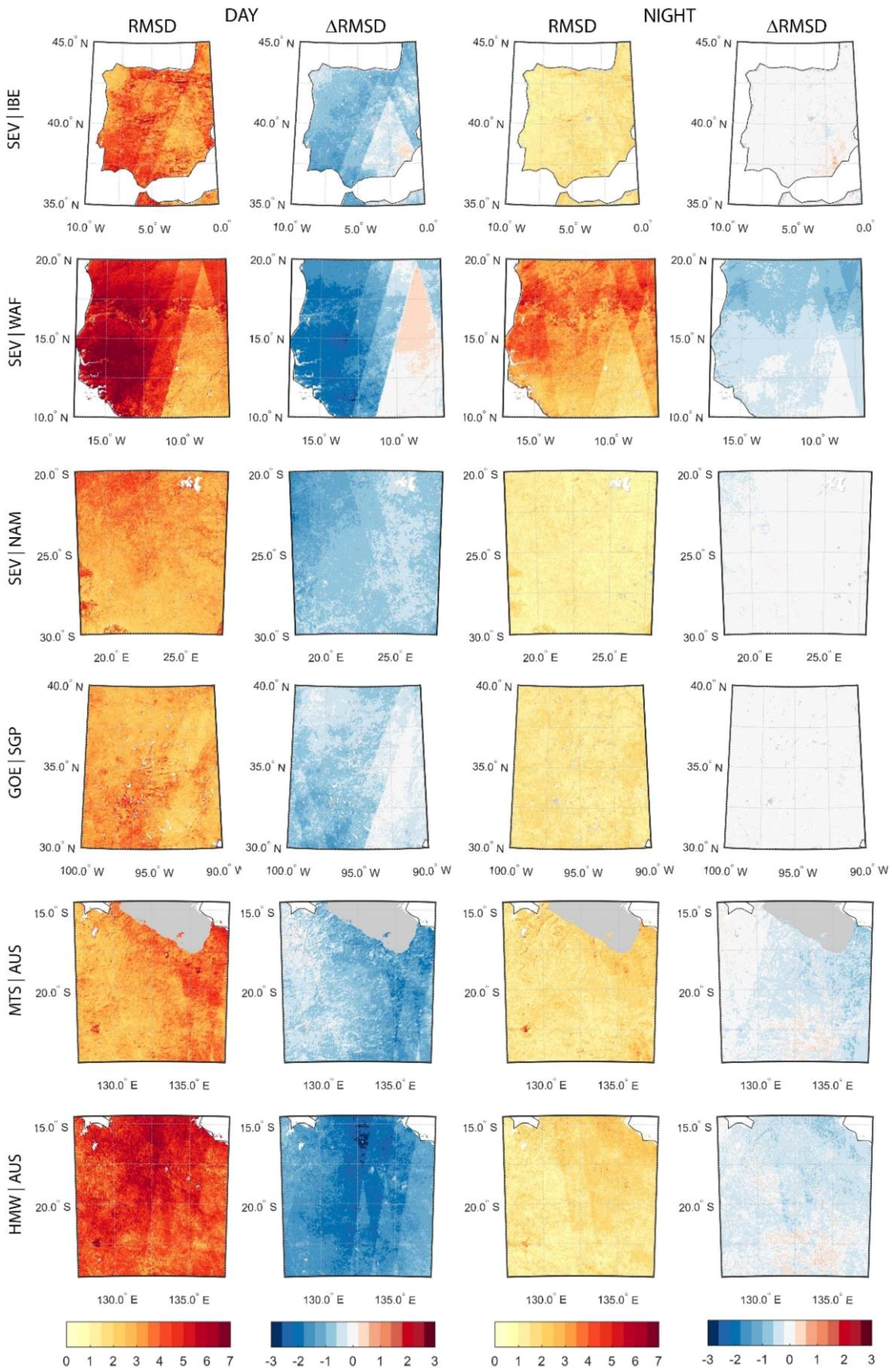
Figure 9.
Examples of LST (a,b) as retrieved by SEVIRI and respective angular corrections to nadir (T-T0 = ΔLST) as given by the Kernel model (c,e) and the Kernel-Hotspot model (d,f), for the 15th of July of 2016 at 00:00 UTC (a,c,e) and 12:00 UTC (b,d,f). Cloudy land pixels are represented in grey.
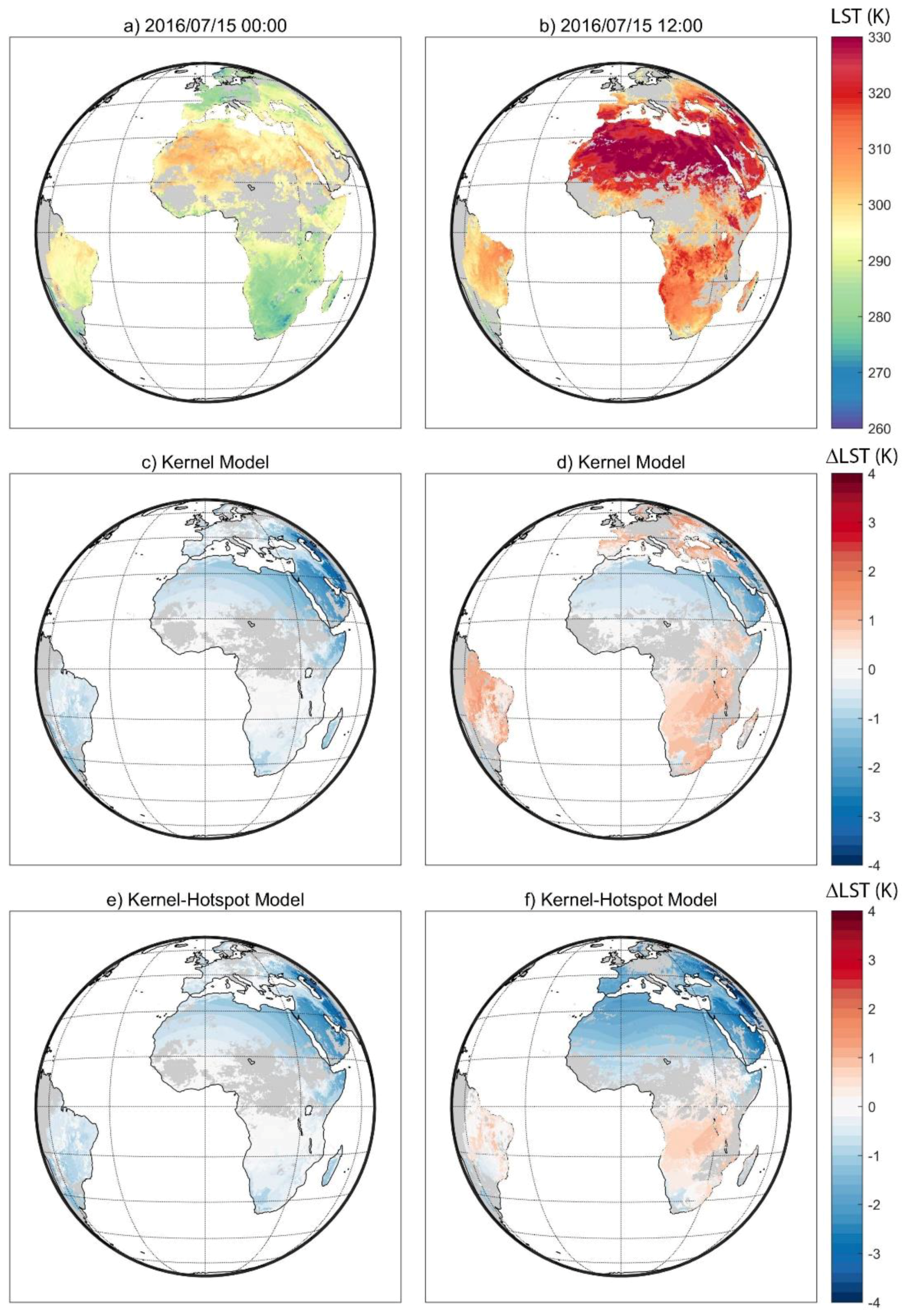
Figure 10.
As in Figure 9 but at 09:00 UTC (a,c,e) and 15:00 UTC (b,d,f).
Figure 10.
As in Figure 9 but at 09:00 UTC (a,c,e) and 15:00 UTC (b,d,f).


Table 1.
Regression coefficients of the bias correction performed between MODIS and SEVIRI land surface temperature (LST) products. The number of observations used in the regression, Root Mean Square Error (RMSE) of the regression and overall bias between MODIS and SEVIRI (as SEVIRI minus MODIS) for each cluster are also shown.
| Cluster | Regression Coefficients | Number of Observations | RMSE of Regression (K) | Bias (K) SEV-MOD | |
|---|---|---|---|---|---|
| α | β | ||||
| C1 | 0.963 | 10.822 | 777,309 | 1.09 | −0.03 |
| C2 | 0.961 | 10.734 | 2,857,306 | 1.00 | 0.39 |
| C3 | 0.931 | 19.337 | 4,215,109 | 1.08 | 0.76 |
| C4 | 0.929 | 19.803 | 3,382,424 | 1.09 | 0.87 |
| F1 | 0.917 | 23.894 | 4,096,421 | 0.98 | 0.20 |
| F2 | 0.948 | 15.256 | 960,060 | 0.94 | −0.10 |
| F3 | 0.948 | 14.609 | 578,180 | 1.22 | 0.35 |
| F4 | 0.929 | 20.332 | 3,177,814 | 0.98 | 0.10 |
| S1 | 0.954 | 13.019 | 626,771 | 1.08 | 0.34 |
| S2 | 0.947 | 14.744 | 6,315,089 | 1.00 | 0.61 |
| S3 | 0.965 | 9.478 | 5,336,698 | 1.05 | 0.35 |
| S4 | 0.899 | 28.847 | 5,724,226 | 1.01 | 0.73 |
| S5 | 0.944 | 15.319 | 6,955,354 | 1.20 | 0.92 |
| D1 | 0.951 | 12.328 | 3,899,579 | 1.30 | 1.82 |
| D2 | 1.023 | −8.363 | 50,020,779 | 1.17 | 1.66 |
© 2018 by the authors. Licensee MDPI, Basel, Switzerland. This article is an open access article distributed under the terms and conditions of the Creative Commons Attribution (CC BY) license (http://creativecommons.org/licenses/by/4.0/).
Share and Cite
MDPI and ACS Style
Ermida, S.L.; Trigo, I.F.; DaCamara, C.C.; Pires, A.C. A Methodology to Simulate LST Directional Effects Based on Parametric Models and Landscape Properties. Remote Sens. 2018, 10, 1114. https://doi.org/10.3390/rs10071114
AMA Style
Ermida SL, Trigo IF, DaCamara CC, Pires AC. A Methodology to Simulate LST Directional Effects Based on Parametric Models and Landscape Properties. Remote Sensing. 2018; 10(7):1114. https://doi.org/10.3390/rs10071114
Chicago/Turabian StyleErmida, Sofia L., Isabel F. Trigo, Carlos C. DaCamara, and Ana C. Pires. 2018. "A Methodology to Simulate LST Directional Effects Based on Parametric Models and Landscape Properties" Remote Sensing 10, no. 7: 1114. https://doi.org/10.3390/rs10071114
Note that from the first issue of 2016, this journal uses article numbers instead of page numbers. See further details here.