Integrating Airborne Hyperspectral, Topographic, and Soil Data for Estimating Pasture Quality Using Recursive Feature Elimination with Random Forest Regression

Abstract

Accurate and efficient monitoring of pasture quality on hill country farm systems is crucial for pasture management and optimizing production. Hyperspectral imaging is a promising tool for mapping a wide range of biophysical and biochemical properties of vegetation from leaf to canopy scale. In this study, the potential of high spatial resolution and airborne hyperspectral imaging for predicting crude protein (CP) and metabolizable energy (ME) in heterogeneous hill country farm was investigated. Regression models were developed between measured pasture quality values and hyperspectral data using random forest regression (RF). The results proved that pasture quality could be predicted with hyperspectral data alone; however, accuracy was improved after combining the hyperspectral data with environmental data (elevation, slope angle, slope aspect, and soil type) where the prediction accuracy for CP was R²_CV (cross-validated coefficient of determination) = 0.70, RMSE_CV (cross-validated root mean square error) = 2.06%, RPD_CV (cross-validated ratio to prediction deviation) = 1.82 and ME: R²_CV = 0.75, RMSE_CV = 0.65 MJ/kg DM, RPD_CV = 2.11. Interestingly, the accuracy was further out-performed by considering important hyperspectral and environmental variables using RF combined with recursive feature elimination (RFE) (CP: R²_CV = 0.80, RMSE_CV = 1.68%, RPD_CV = 2.23; ME: R²_CV = 0.78, RMSE_CV = 0.61 MJ/kg DM, RPD_CV = 2.19). Similar performance trends were noticed with validation data. Utilizing the best model, spatial pasture quality maps were created across the farm. Overall, this study showed the potential of airborne hyperspectral data for producing accurate pasture quality maps, which will help farm managers to optimize decisions to improve environmental and economic benefits.

1. Introduction

Pasture quality is a growing concern because it is a critical constraint for achieving optimal growth and performance for animal production [1]. To meet the nutritional requirements of animals, high quality pasture needs to be maintained on farms. Therefore, being able to accurately assess pasture quality is essential to maintain high quality feed throughout the year. Typically, the assessment of pasture quality, crude protein (CP) and metabolisable energy (ME), is derived from laboratory analysis; however, this method takes significant time and expense, which means these variables are not often measured.

The wider application of remote sensing techniques for precision grassland management is restricted due to heterogeneous pasture [2]. However, substantial progress has been made with sensors and analytical techniques in recent years that can provide comprehensive, site-specific, quantitative information for grasslands. Full range hyperspectral sensors utilize contiguous narrow spectral measurements of reflected light, which has the potential to capture strong narrow absorptions features caused by chemical bonds present in biochemicals of interest [3,4]. Subsequently, it has proved a powerful tool to quantify a wide range of grassland biophysical; biomass [5], dead vegetation fraction [6], and biochemical attributes such as: biomass, leaf area index [7,8], nitrogen [9,10,11], phosphorus [12], fiber [13,14], polyphenols [15], and cellulose [16].

Although a great variety of vegetation indices (VI’s) are widely used to estimate various vegetation properties from reflected light, their potential is limited in the quantification of biochemicals under heterogeneous grassland systems [17]. Compared to the full spectrum-based models, the performance of models based on VI’s was inconsistent due to different canopy characteristics [18]. Subsequently, multivariate statistics have been proposed to extract comprehensive information. For instance, Biewer et al. [19] found that compared to VIs, a full spectrum approach had shown strong correlation with forage quality variables such as CP, ME, ash, and acid detergent fibre (ADF) in mixed swards. Utilizing full spectrum data yielded higher accuracy than optimal narrowband VIs for estimating N concentration and biomass yield in bioenergy cropping systems [18]. Partial least squares regression (PLSR) is a widely used chemometric approach for quantifying pasture macronutrients [20] and quality [14,19] from hyperspectral data because it effectively addresses the problems of overfitting and collinearity. However, canopy reflectance data may be confounded by factors such as soil background, canopy structure, illumination, and viewing geometry, which leads to non-linear and complex relationships [21]. Consequently, Ramoelo et al. [22] suggested the use of non-linear algorithms and showed that kernel-based PLS (KPLS) is more powerful than traditional/linear PLS for estimating N and P concentrations of grass in heterogeneous savannah ecosystems. Verrelst et al. [23] highlighted the importance of non-linear regression methods to retrieve vegetation properties from remote sensing data. In recent years, machine-learning approaches gained in popularity because of their flexibility in explaining non-linear complex relationships without considering any statistical assumptions. Among the machine learning algorithms, random forest (RF) gained more importance in hyperspectral remote sensing due to its capability to deal with complex relationships [24].

The relationships could be improved if the hyperspectral data was combined with the environmental variables, as pasture quality is influenced by environmental factors [22]. Soil fertility is a key driver for pasture growth and quality; therefore, adequate supplies of nutrients through regular and balanced fertilization is essential to maintain high quality pasture. In addition to soil fertility, pasture quality varies spatially on hill country farms due to the impact and interactions of multiple influencing conditions, including topography (elevation, slope angle, and slope aspect), environmental factors (temperature, solar irradiation, rainfall, soil type, and soil moisture), and botanical composition [25]. Pasture quality is also dependent on agronomic management practices, such as stocking rate, pasture cover at set stocking, the shearing policy, and weaning date [26].

Since hyperspectral data carries redundant information, selecting relevant spectral variables in the modelling process could improve prediction accuracy and model robustness [27,28]. Although several approaches have been proposed for selecting the best features, Grenitto et al. [29] highlighted that recursive feature elimination (RFE) combined with RF could provide unbiased and stable results with improved accuracy. However, to our knowledge, this method was not investigated for estimating pasture quality attributes, motivating the present study, which aims to test the potential of multiple source information combined with RF–RFE to describe pasture quality (CP and ME) information. Also, the important hyperspectral and environmental variables will be screened using RF–RFE.

2. Materials and Methods

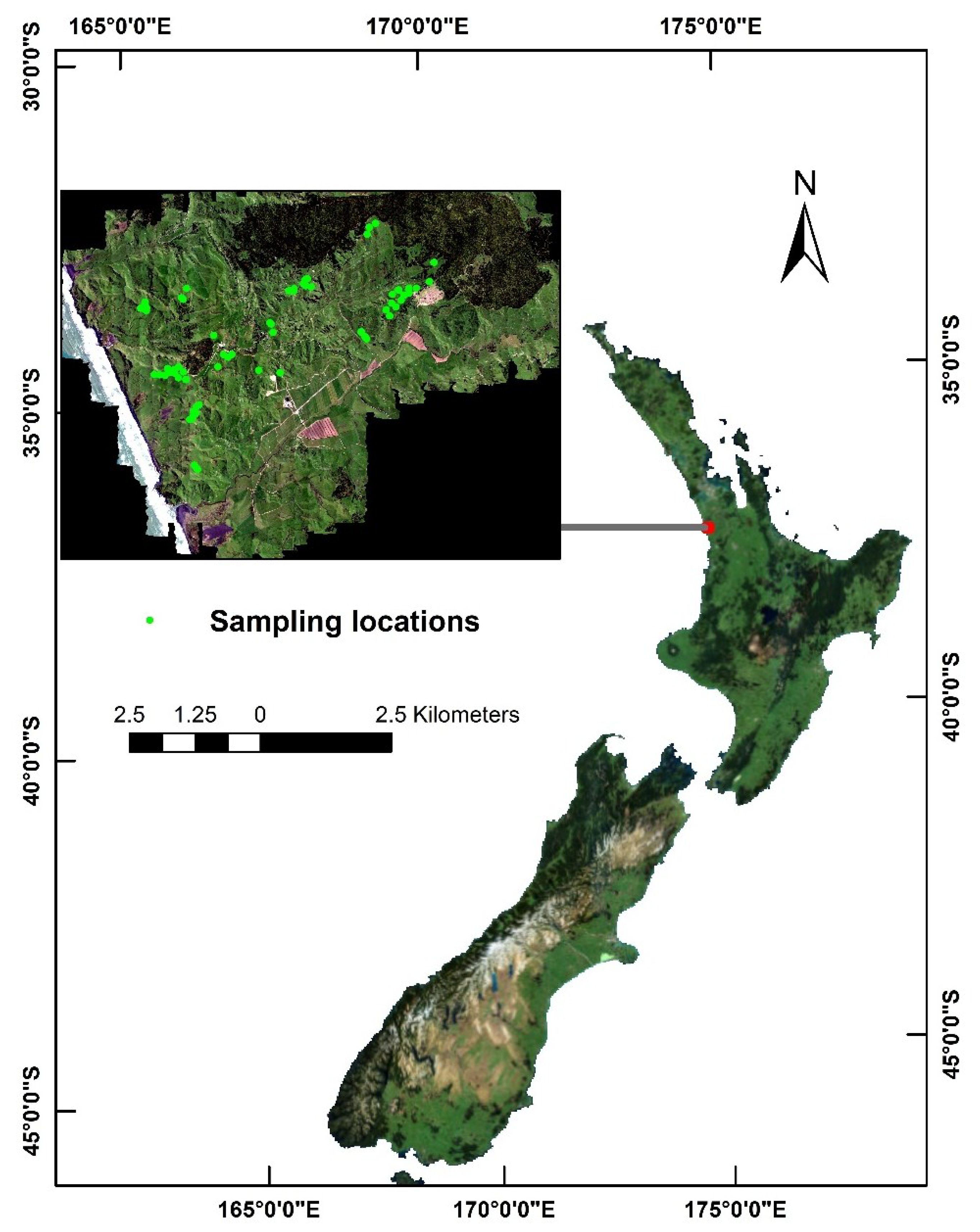
The study area, Limestone Downs, was located at Port Waikato (37°28.665′S, 174°45.540′E) in the northwest of New Zealand where mixed pasture is grown throughout the year (Figure 1). The total study area comprises approximately 3148 ha which classified into 190 paddocks with different sizes ranging from 1.5 to 41 ha. Perennial ryegrass (Lolium perenne L.) and white clover (Trifolium repens L.) are the dominate species, and a small proportion of kikuyu grass (Cenchrus clandestinus), dandelion (Taraxacum officinale), and catsear (Hypochaeris radicata) are also present. The study area is conventionally used for sheep and beef production. The mean annual precipitation and temperature ranges between 1250–1500 mm and 14.1–16 °C for the period 1971–2000. This study was conducted during the spring season where optimal conditions (temperature, rainfall, and sunshine) prevail for pasture growth.

A full-spectrum, pushbroom AisaFENIX (Specim Ltd., Oulu, Finland) hyperspectral imaging system was used in the study. The sensor measures upwelling radiance from 370 to 2500 nm as Digital Numbers (DN) with a spectral interval of 3.5–12.2 nm. The AisaFENIX sensor (Specim, Oulu, Finland) has a Field of View (FOV) of 32.2°, as well as an Instantaneous Field of View (IFOV) of 0.084°. The hyperspectral imaging system was mounted on a single-engine, fixed-wing aircraft which was flown at an elevation around 660 m to ensure ground sampling distance of approximately 1 m. To know the position of each pixel, the hyperspectral imaging system was coupled with an RT Oxford Survey+ Ltd., Global Navigation Satellite System (GNSS) and an Inertial Measurement Unit (IMU). The image was collected between 10:30 and 12:00 New Zealand local time on 24th October 2014. The digital numbers (DN) were converted into radiance (W m⁻² sr⁻¹) using factory provided radiometric calibration coefficients in CaliGeoPRO software (Specim, Finland). Surface reflectance values were obtained from radiance data using ATCOR4 (ReSe Ltd., Wil, Switzerland), which used geographic, temporal, and atmospheric parameters [30].

Within the study area, based on the access, 150 sites were selected for pasture using stratified random sampling. Elevation and slope angle variables were used as strata, and random sites were then selected from each strata. Since paddocks were not used as a basis for selecting the sites, the total sites came from 72 paddocks, where some of the sites fall under individual paddocks and the remainder from multiple locations of a paddock. Following the aerial campaign, at each of the 150 sites, a 0.5 × 0.5-m quadrat was placed on the ground and a pasture sample harvested to ground level using battery-powered hand shears. The cut samples were immediately placed in a labelled polythene bag, sealed, and stored in a chiller box. These boxes were then transported to an analytical laboratory (Analytical Research Laboratories Ltd., Napier, New Zealand) for immediate determination of CP and ME.

In addition to hyperspectral data, site elevation, slope angle, slope aspect, as well as soil type (Figure 2) were included in the analysis. Elevation, slope angle, and slope aspect maps were generated with a linear filter [31] on a low resolution (5 m) Light Detection And Ranging (LiDAR) Digital Terrain Model, captured in 2010. Soil type information was gathered from Massey University soil map archives. Based on the evolution of New Zealand soils, soil taxonomy, and local knowledge, a new classification was developed [32]. This study included 16 soil types: oxidic granular, allophanic brown, deep orthic, humic gley, humic organic, mottled orthic recent, orthic allophanic, orthic brown, orthic gley, orthic gley and sandy brown, rendzic melanic, sandy brown, sandy gley, sandy raw, sandy recent and typic oxidic granular (Figure 2). Allophanic soils are low density and low fertile which has ability to retain phosphorus in high. Brown soils dominated with clay minerals cover 43% of New Zealand. Gley soils are highly fertile and rich in organic matter. Similar to gley soils, organic soil is rich in organic matter and extremely acidic. Granular soils developed from andesitic to rhyolitic volcanic deposits with a moderate amount of weathering products, such as kaolinite. Melanic soils are highly fertile, with large populations of microorganisms. Oxidic soils are well-developed soils weathered from volcanic deposits, which are dominated with iron and aluminum oxides. Recent soils cover 6% of New Zealand, which is developed on volcanic tephra, and these soils are dominated by secondary illite minerals. The auxiliary data were resampled and co-registered with the hyperspectral image using a nearest neighbor interpolation method.

The spectral and environmental data in the corresponding sampling locations were extracted from a window size of 3 × 3 (9 m²). The mean value from each window was considered as a response variable. The reflectance data was converted into first derivative reflectance (FDR) using Savitzky-Golay filter to highlight the subtle overlapping absorption peaks. Following the transformation, random forest regression (RFR) was applied to develop relationships between pasture quality and hyperspectral and environmental data. The soil data was converted into binary and stacked with the remaining variables. Since the full data contains different data types, scaling was performed, where each variable value was divided by its standard deviation. For the model development, 60% (n = 90) of total samples were selected, and the remaining 40% (n = 60) were used for validating the model performance. RF is an ensemble learning technique proposed by Brieman and Leo [32].

RF is a collection of several decision trees where each tree is constructed independently with random samples (n) from the training data. Random samples were drawn with the replacement from the training data using a bootstrap aggregating (bagging) method, which was found to be a more robust method for obtaining a stable model and helped to avoid overfitting [33]. Usually, 64% of training data is selected as in-bag data, and the remaining 36% were referred to as out-of-bag (OOB) data. At each node, a random subset of variables were selected. RFR learns the behaviour of the selected m variables and finally selects best performing variables using least square error criteria. The final prediction results were obtained by averaging the predicted results from all trees.

For constructing the model, it is necessary to tune two important parameters: the number of variables at each split and the number of trees. Each split of the tree is determined using a randomized subset of the variables (the default is 1/3 of the total number of variables) at each node [34]. The number of trees was optimized using root mean square error (RMSE) and tested on different population of trees ranging from 50 to 448 using every 10th interval.

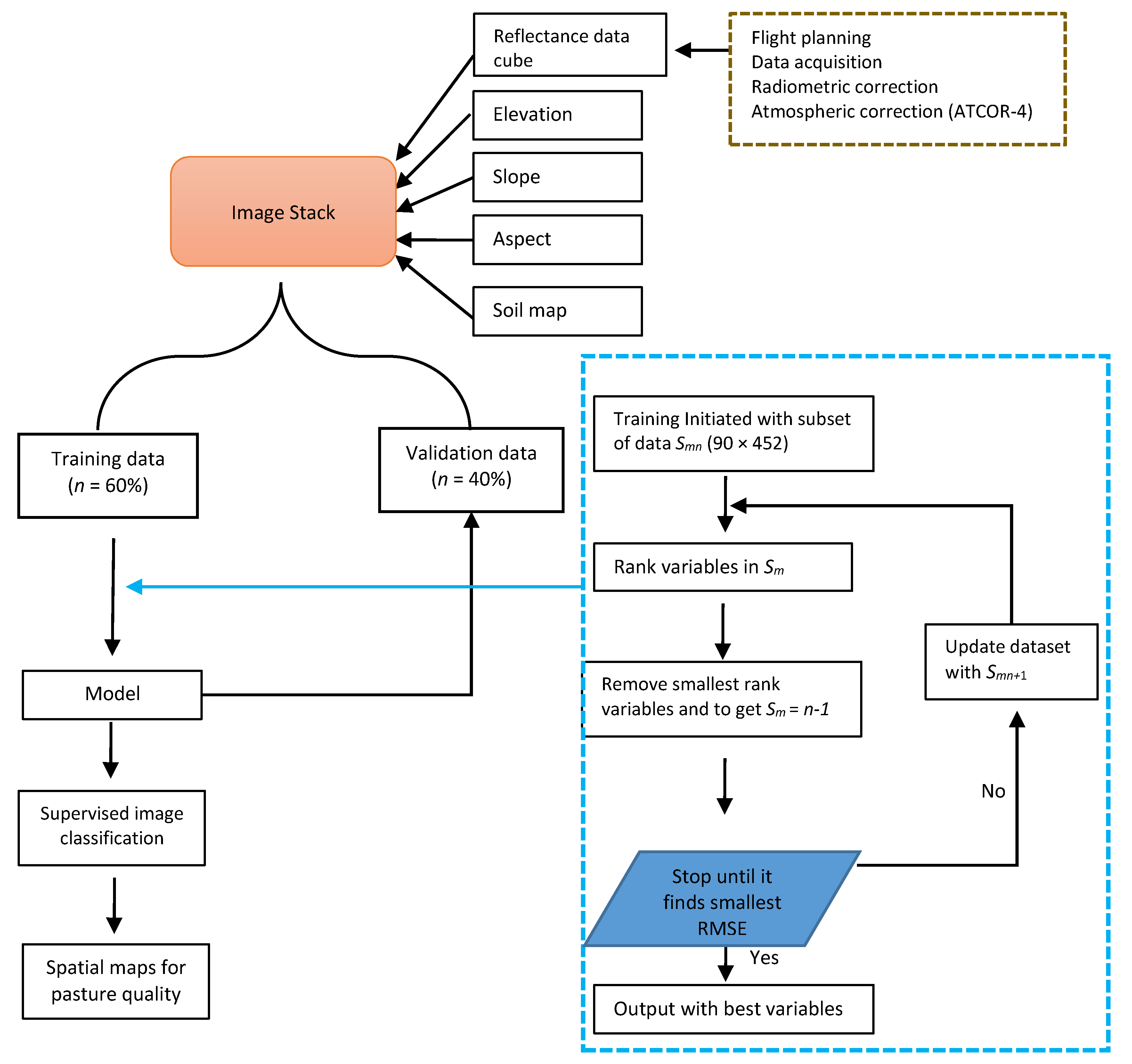
The RFE is a wrapper-based feature-ranking algorithm that searches within the space for optimal subset by performing optimization algorithms [35]. The construction of the model initiates with training data, and variables are then ranked according to their importance (Figure 3). While constructing the decision trees, each variable in the OOB data is randomly permuted. After this, RMSE values were calculated for OOB data, and the permuted variables were estimated (Figure 3). Based on the RMSE values, one variable was removed, and a new RF model was created using the remaining variables. This process was recursively applied until only one variable remained as input [36]. During the process of elimination, 10-fold cross validation was implemented to optimize the variable selection and to ascertain the standard deviation of error. In the recursion process, the model with minimum RMSE and with least standard deviation error was set as the optimum model; if it finds another model with a different subset of variables, it automatically updates and ranks. Finally, it selects the best variables yielding the smallest RMSE.

The goodness of fit of the developed regression models were evaluated by calculating the cross-validated coefficient of determination (R²_CV), cross-validated root mean square error (RMSE_CV), and cross-validated ratio to prediction deviation (RPD_CV).

$${\mathrm{RMSE}}_{\mathrm{CV}}=\sqrt{{\displaystyle \sum }_{i=1}^N\frac{{\left(\widehat{y_i}-y\right)}^2}{N}}$$

$${\mathrm{RPD}}_{\mathrm{CV}}=\frac{\mathrm{SD}\left(y\right)}{{\mathrm{RMSE}}_{\mathrm{CV}}}$$

where $\widehat{y}$ is the predicted values, y is the observed value, and N is the number of samples. SD(y) refers to standard deviation of measured y. Models with RPD ≥ 2 predict well with reliable estimates [14]. Pasture quality maps were generated using the best model.

The final maps were created using masking. For this, the land surface cover maps were created by classifying the hyperspectral image. The land cover types included in this study are forest, bush, pasture, and non-vegetation areas. The classification was performed using supervised algorithm, support vector machine (SVM). SVM is a robust classification method widely used for hyperspectral imagery [37]. We have used radial basis function; their parameters (cost and gamma) were optimized using 5-fold cross-validation. High-resolution RGB images were used as a georeference for selecting the training pixels from the hyperspectral image. The training model was then used to extrapolate the hyperspectral image across the landscape. Model development, creating pasture-quality maps, and classification of hyperspectral image was performed in MATLAB^® environment.

3. Results

The pasture quality attributes were estimated from the samples collected in the field. The descriptive statistics of pasture quality values for the calibration model are summarized in

Table 1. Descriptive statistics: mean, standard deviation (std), minimum (min), maximum (max), and coefficient of variation (CV) pasture quality data was used to build a calibration model.

Pasture Quality	Mean	std	Min	Max	CV (%)
Crude protein (%)	16.31	3.76	6.06	25.64	23.05
Metabolisable energy (MJ/kg DM)	10.91	1.37	6.00	12.50	12.55

Note: std- standard deviation; CV- coefficient of variation.

. The collected pasture samples had high variability for CP (CV = 23.05%) with a range from 6.06 to 25.64 and high standard deviation (std = 3.76). In contrast, ME exhibited low variability (CV = 12.55%) and a small range (6–12.50) of samples. As expected, a wide range of pasture variability, particularly with CP, exists on hill country farms due to diverse environmental conditions [38].

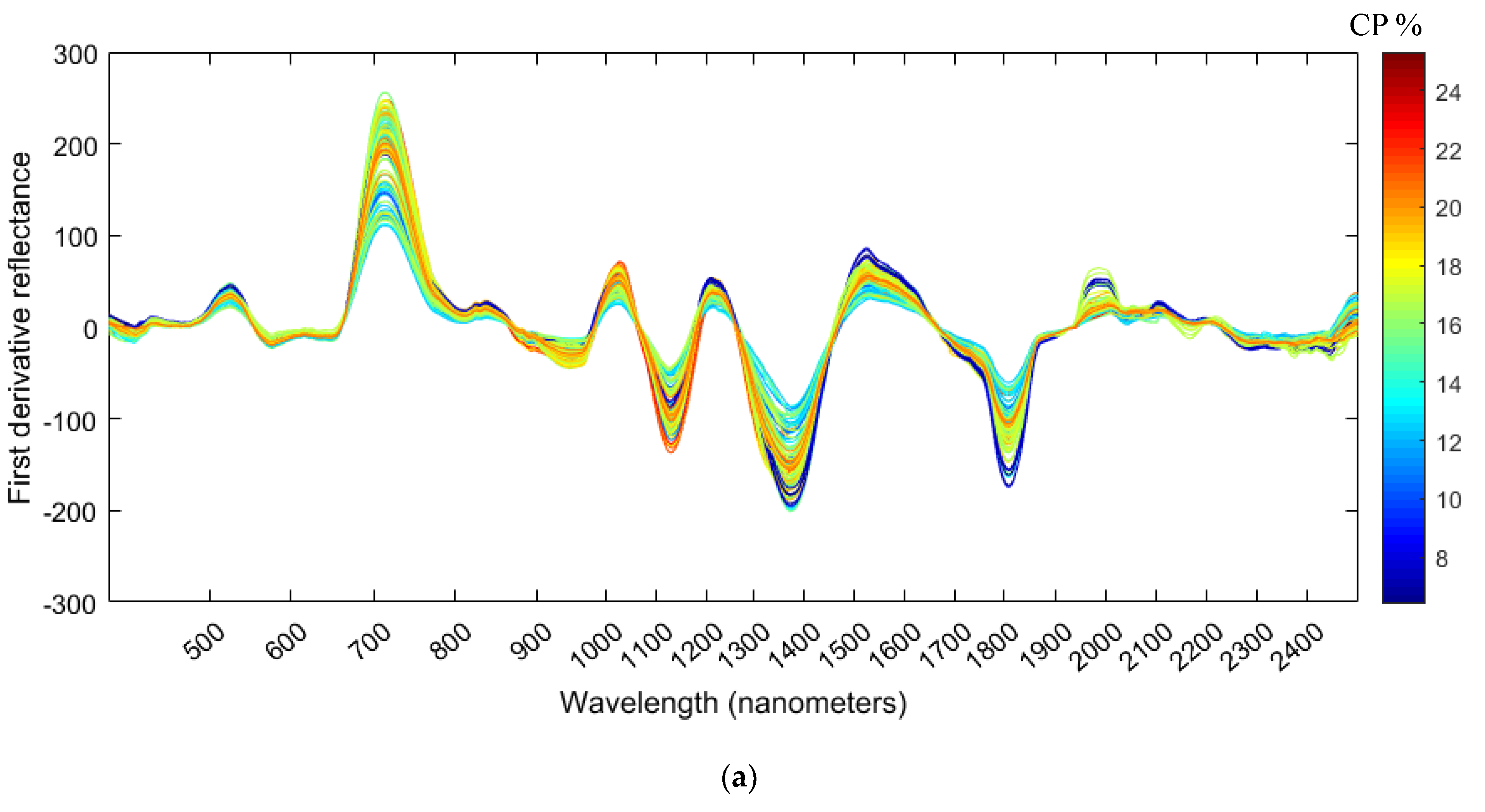
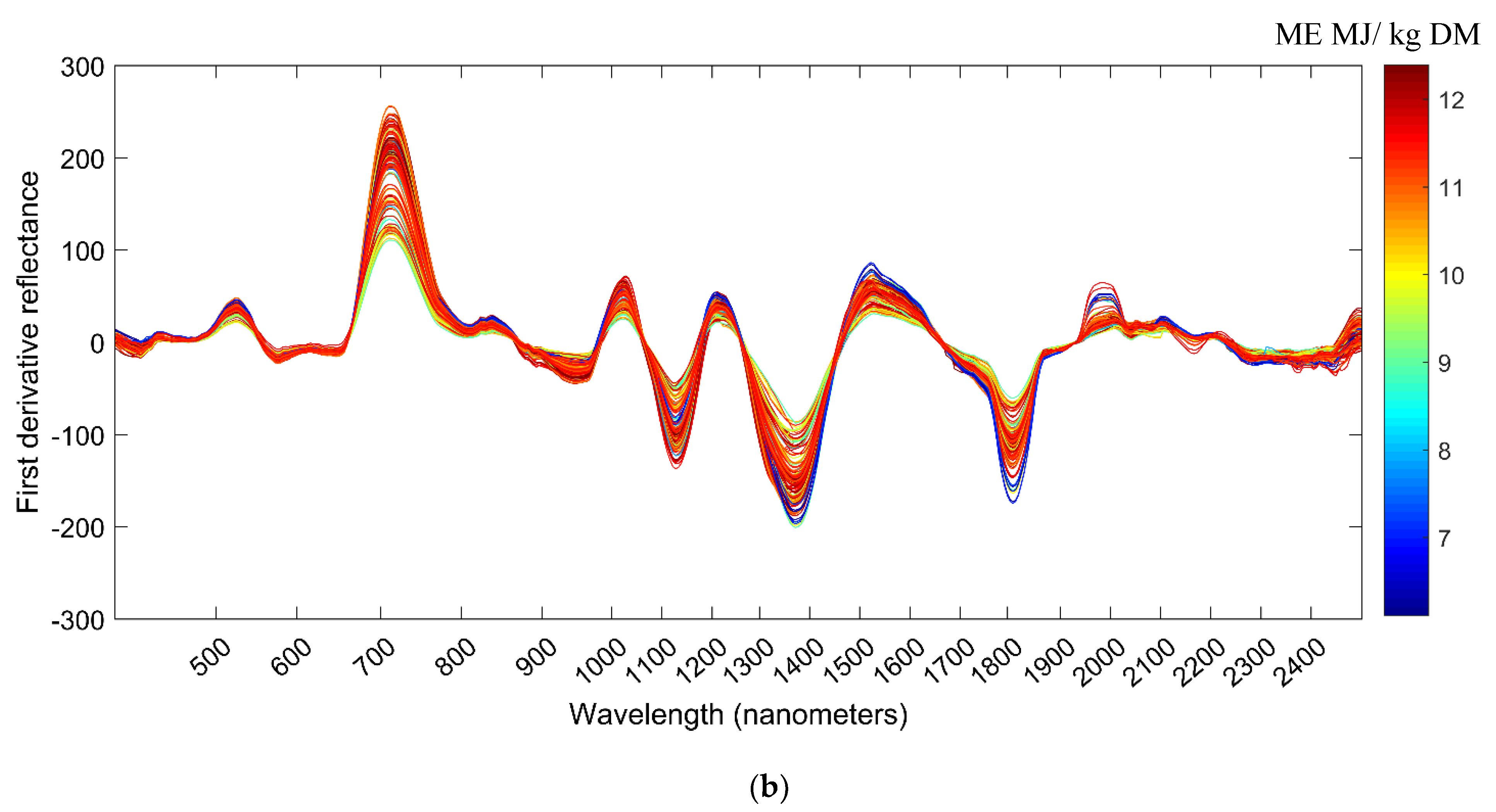
FDR of corresponding pasture samples extracted from the AisaFENIX were presented as a function of pasture quality attributes (CP and ME) in Figure 4.

The magnitude of absorption features are highly variable and complex with relevant pasture quality values. In Figure 4, there are a few distinctive spectral features of high and low pasture quality that can be seen around 1230 nm, 1340 nm, 1550 nm, and 1800 nm. The relationships between spectral data and measured values of CP and ME were shown in

Table 2. Regression model results for crude protein (CP) and metabolizable energy (ME) using airborne hyperspectral imaging. Regression metrics are R²_CV-cross-validated coefficient of determination, RMSE_CV- cross-validated root mean square error, and RPD_CV- cross-validated ratio to prediction deviation.

Pasture Quality	Variables	R2CV	RMSECV	RPDCV	R2P	RMSEP	RPDP
CP	Full-spectrum	0.66	2.24	1.68	0.63	2.20	1.65
CP	Elevation, slope and aspect and soil type	0.31	3.13	1.20	0.27	3.81	0.95
CP	FS, elevation, slope, aspect and soil type	0.70	2.06	1.82	0.70	2.01	1.80
CP	Selected variables a	0.80	1.68	2.23	0.78	1.72	2.11
ME	FS	0.61	0.85	1.62	0.61	0.86	1.64
ME	Elevation, slope and aspect and soil type	0.35	1.10	1.24	0.32	1.22	1.15
ME	FS, elevation, slope, aspect and soil type	0.75	0.65	2.11	0.77	0.63	2.23
ME	Selected variables b	0.78	0.61	2.25	0.79	0.60	2.35

Note: FS—Full spectrum; ^a elevation, slope, soil type, and spectral features from Figure 5a. ^b slope, soil type and spectral features from Figure 5b.

. The results from this study indicate that CP was predicted with high accuracy from hyperspectral data using RF technique (R²_CV = 0.66, RMSE_CV = 2.24, RPD_CV = 1.68). However, the accuracy was slightly improved (R²_CV = 0.70, RMSE_CV = 2.06, RPD_CV = 1.82) by adding environmental variables (elevation, slope angle, slope aspect, and soil type) (Table 2). The pasture ME was predicted with an R²_CV of 0.61, RMSE_CV = 0.85, and RPD_CV = 1.62 with hyperspectral data alone. The prediction accuracy of ME increased dramatically after including environmental variables (R²_CV = 0.75, RMSE_CV = 0.65, and RPD_CV = 2.11). Separate regression models were also created to assess the impact of only environmental variables on both CP and ME. This resulted in a relatively low accuracy models (0.35 ≥ R²_CV ≤ 0.31).

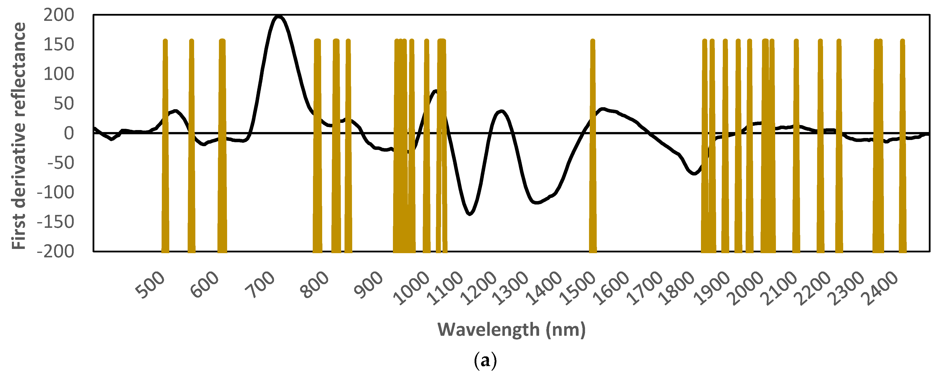
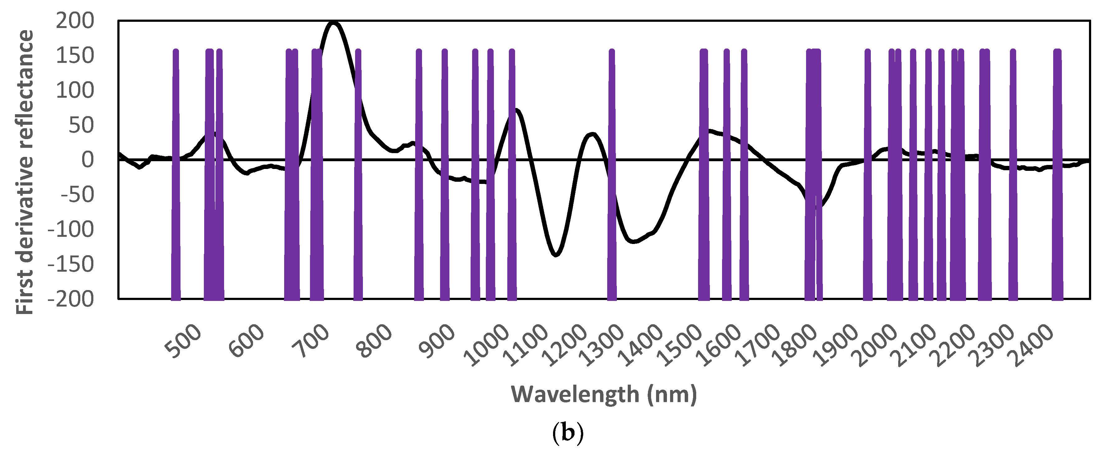
When feature selection was performed using RF–RFE, the accuracy was further improved for both CP and ME. It is worth noting that the improvement was higher in the case of the CP model when compared to the ME model. The calibration model prediction results were consistent with validation results, though the validation results were slightly lower than the calibration results. Only 7–8% of hyperspectral variables were selected as important for describing CP and ME, which are present across the electromagnetic spectrum, though the majority of them are concentrated in the short wave infrared (SWIR) region. The selected important wavebands by RF–RFE for each pasture quality attribute are shown in Figure 5. For CP, the sensitive spectral bands are 505–554, 609, 612, 784, 787, 818, 822, 842, 932, 939, 946, 959, 1000, 1500, 1935, 2013, 2018, 2035, 2107, 2178, 2234, 2344, and 2420 nm. The sensitive spectral bands for ME are 517–520, 643, 653, 684, 691, 753, 849, 890, 939, 963, 1017, 1276, 1512–1520, 1618, 1785, 1796, 1802–1808, 1935, 1996, 2013, 2051, 2090, 2123, 2173, 2239, 2305, 2415, and 2420 nm. The pasture attributes CP and ME have moderate intercorrelation (R² = 0.38) and are found with few common bands (939, 1935, 2013, 2420 nm).

In both CP and ME, the included environmental variables were found to have significant influence on model performance with improved accuracy.

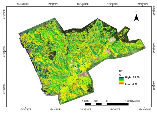
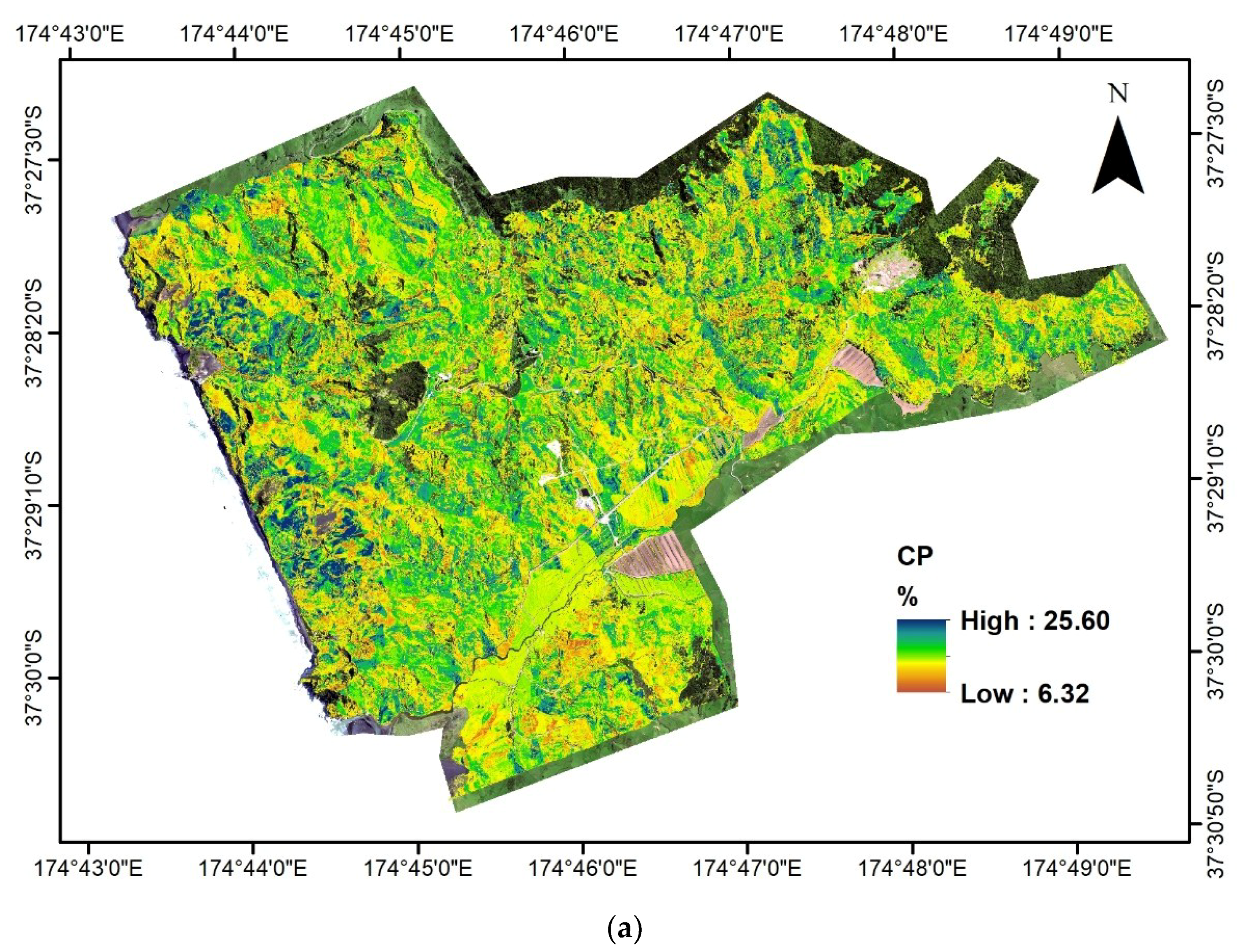
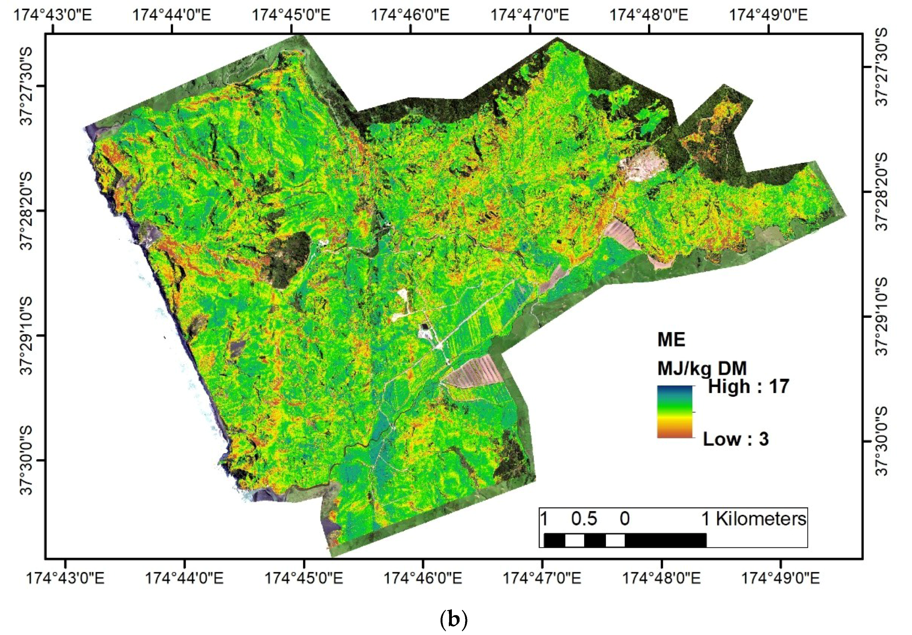
The prediction models with the highest R²_CV values were to create raster maps, depicting the spatial pattern of pasture quality (Figure 6). The spatial maps of CP and ME were masked using the land surface classification map from SVM, which is as accurate as 93.4% (overall accuracy). The pasture areas were highlighted with colored pixels and non-pasture areas left empty with a background of RGB image. The range of predicted CP is from 6.32 to 25.60% with high values in the east and west sides of the study area, while the south was dominated with low CP pasture (Figure 6). Compared with CP, ME was less variable across the area with the majority of the area dominated by moderate ME values (Figure 6).

4. Discussion

Airborne hyperspectral imaging has potential for estimating CP and ME accurately and over large spatial extents which enables continuous spatial maps to be created. In this study, a hill country farm was imaged with an airborne hyperspectral system which produced accurate estimates for CP (RPD_CV = 2.23) and ME (RPD_CV = 2.25) of heterogeneous mixed pasture. The successful application of this technology in pasture quality is not surprising, as pointed out by previous studies [14,16,19,39]; however, the approach used in this study improved the prediction results by integrating the hyperspectral and environmental data-combined machine-learning algorithms. Such knowledge of the landscape could inform pasture and herd management decisions to improve animal production and assist in land stewardship efforts.

In Figure 4, the pasture quality relevant features were not very distinct. This is due to the fact that the variation in canopy reflectance was primarly influenced by direct and indirect confounding factors such as canopy structure, solar/viewing geometry, soil background, broad water absorptions, while the contribution from vegetation chemistry is very small (2–4%) [40]. These multiple factors also impede the attribute estimation to some extent, though the proposed approach produced accurate estimates. Further investigation is required to break down the individual influence from these factors on pasture quality.

Although the pasture was characterized by heterogeneity, RF has accounted for maximum explanation on pasture quality from the hyperspectral data. Many studies suggest that RF may be more powerful than the traditional multivariate regression methods as it extracts complex, non-linear information from the spectral data [24,27]. In this study, RF accounted for >70% of the variability in CP and ME from the hyperspectral data alone. When combined with the topographic and soil data, the RF–RFE approach showed an improvement in the prediction accuracy. The latter indicates the importance of considering environmental data for estimating pasture quality. Similarly, Ramoelo et al. [22] attempted to combine proximal hyperspectral data with environmental data to predict nitrogen and phosphorus concentration of grass in a savannah ecosystem using non-linear-PLSR, and the researchers found improved results over the hyperspectral data alone. From the results obtained in this study, we recommend the use of spectral and environmental variables together to provide improved prediction accuracy.

RF–RFE is capable of selecting important spectral and environmental features that are sensitive to pasture quality and improved the accuracy levels. Similarly, Granitto et al. [29] used RF–RFE for analysing high dimensional data and found it to be an efficient feature selection method, far better than traditional methods. Other researchers [21,41] found that considering noisy variables could interfere with model performance, which leads to over-fitting. Therefore, important relevant features need to be selected for robust estimates. As seen in Figure 5, the selected spectral bands are scattered over the whole spectrum indicating the importance of full-spectrum. The selected bands for each quality attribute are different because of the contrasting chemical composition of each attribute. However, bands at 939, 1935, 2013, and 2420 nm are mutually selected in both cases. This might be due to the presence of common functional bonds; hence, both quality attributes are noticed with correlation (Table 2). The band 1935 nm is influenced by broad water absorption centered at 1940 nm [40]. With both quality attributes, the spectral region from 500–770 nm related electronic transitions caused by pigment absorptions, such as chlorophyll, xanthophyll, and carotenoids. Clustering of sensitive bands are located in the SWIR region, which are mainly characterized by fundamental overtones and harmonics of O–H, C–C, C–H, and N–H [3,42]. In CP, the majority of the selected bands (932, 1000, 1500, 1935, 2035, 2178, 2234 and 2344 nm) are closely assigned with bond vibrations of protein and nitrogen molecules [3]. Fundamentally, ME is mainly composed of crude fibre [43]; therefore, the majority of the selected bands (1017, 1276, 1512–1520, 1618, 1785, 1796, 1802–1808, 1935, 2090, 2123, 2239, 2305, 2415 and 2420 nm) are associated with vibrations of lignin, cellulose, and hemicellulose [3].

Pasture quality appeared to be correlated with topographic variables and soil type, which indicates that these variables are also one of the key drivers to influence pasture quality (Table 2). This leads to improved accuracy by combining the hyperspectral and environmental data (Table 2). In this study, a wide range of soil types with different nutrient levels are present across the farm, which directly support changes of pasture quality (CP and ME). For example, in Figure 2 and Figure 6, gley soils dominated paddocks distributed with high quality pasture (high ME and optimal CP values) because of high fertility of soils. In contrast, paddocks with allophanic soils show low quality pasture (low ME and CP). Slope variables also positively influenced the pasture quality. Generally, flat regions were associateded with high fertility soils, while hilly regions lost soil fertility due to surface run-off [22]. Although the current study proves the feasibility of mapping pasture quality at local scale, under large-scale environments, the influence of topography and soil type might be different due to the presence of different soil types and environments. Moreover, the relationships might change with seasons due to variable weather conditions and pasture response. Therefore, further investigation is required before utilizing this model for large-scale environments.

Understanding the spatial variability of pasture quality in hill country farms allows for more efficient use of natural resources and improving agronomic management. Both CP and ME exhibited different spatial patterns, reflecting the different factors that influence each attribute. Fertilizer is a key input in hill country farms, as it helps to maintain high quality pasture. Traditional blanket application of fertilizer ignores spatial variability and can result in the application of excessive fertilizer on high-fertility zones and vice-versa on low fertility which can result in the loss of fertilizer into the environment; with fertilizer being such a large investment for farmers, it is important to ensure that the value of that investment is realized as fully as possible. In 2006, Murray and Yule [44] conducted an experiment to test the performance variable rate fertilizer (VRF) over blanket application at Limestone Downs based on broad scale annual pasture production. The single super phosphate was applied through aerial top-dressing aircraft with a controlled ground resolution of 18 m². They reported that the annual pasture production could be increased between 6.5–24.4% by VRF. They also conducted an economic analysis on implementing VRF over the blanket application where they found that this technique could increase 26% annual cash returns per hectare [45]. These findings clearly indicate the potential to improve fertilizer use efficiency and the economic benefits, as well as to reduce the risk of fertilizer wastage contaminating the environment from VRF [38]. From the current research, we are able to quantify pasture quality attributes more accurately at fine scale, which are the better indicators of spatial variability within field over the annual pasture production. These pasture quality maps can provide the necessary inputs for VRF applications. In addition, these comprehensive spatial information quality maps enable the farm managers to ensure proper mineral nutrition of ruminant animals [46].

5. Conclusions

This study evaluated the feasibility of combing the hyperspectral, topography, and soil data to retrieve pasture quality attributes of heterogeneous pasture using RF–RFE. Since the pasture quality variation is driven by many environmental and management factors, our results showed that combining hyperspectral data with generally available environmental factors (elevation, slope angle, and soil type) improved the prediction accuracy in comparison with hyperspectral data alone. This result also confirmed that RF-RFE markedly improved the estimates of pasture quality (RPD = 2.11–2.35) by selecting the most sensitive variables across the spectrum and environmental data. Elevation, slope, and soil type were found as important variables to predict CP while for ME, the same variables with the exception of elevation were found to be significant. The applicability of the proposed approach needs to be investigated on a large-scale where highly variable soil types exist. Overall, the final accurate pasture quality spatial maps allow farmers to optimize their agronomic decisions.