Supervised Classification of Built-Up Areas in Sub-Saharan African Cities Using Landsat Imagery and OpenStreetMap


1
Spatial Epidemiology Lab (SpELL), Université Libre de Bruxelles, B-1050 Brussels, Belgium
2
Department of Geography, University of Namur, B-5000 Namur, Belgium
*
Author to whom correspondence should be addressed.
Remote Sens. 2018, 10(7), 1145; https://doi.org/10.3390/rs10071145
Submission received: 19 June 2018
/
Revised: 12 July 2018
/
Accepted: 16 July 2018
/
Published: 20 July 2018
(This article belongs to the Special Issue Citizen Science and Earth Observation II)
Abstract
:The Landsat archives have been made freely available in 2008, allowing the production of high resolution built-up maps at the regional or global scale. In this context, most of the classification algorithms rely on supervised learning to tackle the heterogeneity of the urban environments. However, at a large scale, the process of collecting training samples becomes a huge project in itself. This leads to a growing interest from the remote sensing community toward Volunteered Geographic Information (VGI) projects such as OpenStreetMap (OSM). Despite the spatial heterogeneity of its contribution patterns, OSM provides an increasing amount of information on the earth’s surface. More interestingly, the community has moved beyond street mapping to collect a wider range of spatial data such as building footprints, land use, or points of interest. In this paper, we propose a classification method that makes use of OSM to automatically collect training samples for supervised learning of built-up areas. To take into account a wide range of potential issues, the approach is assessed in ten Sub-Saharan African urban areas from various demographic profiles and climates. The obtained results are compared with: (1) existing high resolution global urban maps such as the Global Human Settlement Layer (GHSL) or the Human Built-up and Settlements Extent (HBASE); and (2) a supervised classification based on manually digitized training samples. The results suggest that automated supervised classifications based on OSM can provide performances similar to manual approaches, provided that OSM training samples are sufficiently available and correctly pre-processed. Moreover, the proposed method could reach better results in the near future, given the increasing amount and variety of information in the OSM database.
1. Introduction
The population of Africa is predicted to double by 2050 [1], alongside a rapidly growing urbanization. In this context, reliable information on the distribution and the spatial extent of human settlements is crucial to understand and monitor a large set of associated issues, such as the impacts on both environmental systems and human health [2,3,4]. In the 2000s, the remote sensing community took advantage of the availability of coarse-resolution satellite imagery based on the MERIS or the MODIS programs to produce global land cover maps such as GlobCover [5] or the MODIS 500m Map of Global Urban Extent (MOD-500) [6]. Subsequently, Landsat data have been made freely available in 2008 and dramatically reduced the operative cost of high resolution satellite imagery acquisition and processing [7]. This enabled the production of high resolution global land cover maps based on the Landsat catalog, such as the Global Human Settlement Layer (GHSL) [8], Global Land Cover (GLC) [9] or the Human Built-up and Settlements Extent (HBASE) [10].
However, land cover classification in urban areas remains a challenge because of the inherent complexity of the urban environment which is characterized by both intraurban and interurban heterogeneity [11,12]. Because of the complexity associated with the urban mosaic at high resolution, supervised classification methods have been shown to provide the best results [13,14,15]. However, such an approach requires a large amount of training samples to grasp the heterogeneity of the urban environment. As a result, the process of collecting training samples for large-scaled supervised classification becomes an unaffordable task. Additionally, studies have shown that global urban maps suffer from higher rates of misclassifications in developing regions such as Sub-Saharan Africa or South Asia [16] because of the lack of reference data in both quantity and quality.
The training samples collection step can be automated by using existing land cover information in ancillary datasets. Coarser resolution global maps such as GlobCover or MOD-500 have been widely used to identify training sites [16,17]. However, integrating such datasets leads to the introduction of noisy samples which have been shown to decrease the performance of the classifiers. In this context, the increasing availability of Volunteered Geographic Information (VGI) brings new opportunities. Defined as the spatial dimension of the web phenomenon of user-generated content [18], VGI drives a new way of collecting geographic information that relies on the crowd rather than official or commercial organizations. Founded in 2004, OpenStreetMap (OSM) is the most famous of the VGI projects. Initially, the objective was to provide free user-generated street maps [19]. In the following years, OSM became a collaborative effort to create a free and editable map of the whole world which is not limited to the road network [20]. OSM uses a data model based on three object types: nodes (points), ways (polylines or polygons), and relations (logical connections of ways, e.g., a closed way that forms a polygon). Each object is described by at least one key/value pair (a “tag”) [19,20]. This simple data model allows the mapping of a large range of spatial features such as building footprints, points of interest, natural elements, or land use. As a result, and as the database grows, OSM is increasingly used for Land Use and Land Cover (LULC) classification [21,22,23,24]. Furthermore, the increasing data availability and quality enable the use of OSM data to support automated supervised classifications of remote sensing imagery. Shultz et al. successively used OSM objects to fill the data gaps in the global Open Land Cover product based on Landsat imagery [25]. Similarly, Yang et al. used Landsat imagery and training points from OSM to map land use in Southeastern United States with an overall accuracy of 75% [26]. This demonstrates that OSM becomes increasingly relevant to support the training of large-scaled LULC classifications.
However, the use of OSM data also bring new issues to consider, including: (1) its non-exhaustive nature; and (2) the spatial heterogeneity of the contribution patterns across the regions. Indeed, users are more likely to contribute information where they live. According to Coleman et al., economical interest and the “Pride of Place” are among the main factors that encourage people to contribute [27]. Additionally, Juhàsz et al. demonstrated that users are more likely to contribute in specific places such as natural areas and city centers [28]. Furthermore, because of the “Digital Divide” [18] caused by inequalities in access to education and Internet, developing and developed countries does not benefit from the same amount of contributions. As of March 2018, the amount of information (in bytes) in the OSM database was ten times bigger for the European continent than for Africa (http://download.geofabrik.de). Another example of such heterogeneity is that Germany contained two times more bytes of information than Sub-Saharan Africa. However, OSM data availability in developing regions is rapidly increasing over the lastfew years, thanks to local contributors and initiatives such as Humanitarian OpenStreetMap Team (https://www.hotosm.org) or Missing Maps (https://www.missingmaps.org). In fact, Africa is the continent where contributions are increasing at the highest rate since 2014. This makes OSM increasingly relevant in developing regions such as Sub-Saharan Africa.
This paper focuses on the use of OSM to collect training samples for the classification of built-up and non-built-up areas in Landsat scenes of ten Sub-Saharan African urban agglomerations. To support global urban mapping, our research aimed to answer the following questions: What information can be extracted from the OSM database to collect built-up and non-built-up training samples? What post-processing must be applied? What performance loss can we expect compared to a strategy based on a manually digitized dataset? Finally, what is the practicability of this approach in the context of a developing region such as Sub-Saharan Africa?
2. Materials and Methods
2.1. Case Studies
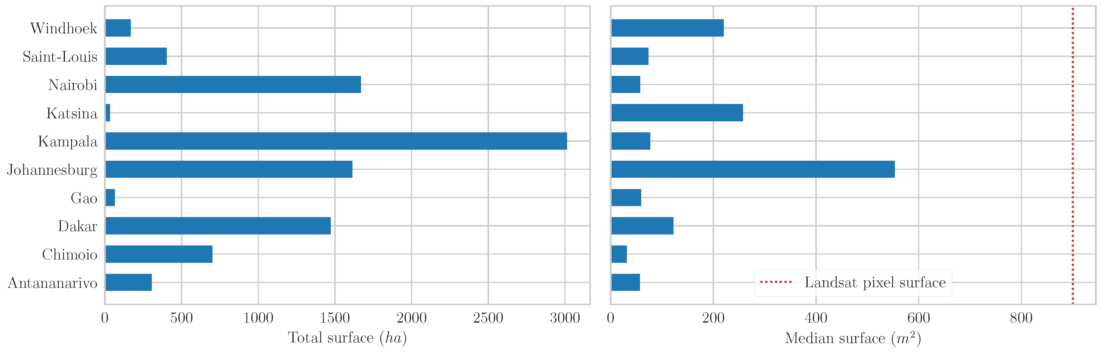
As stated previously, the spectral profiles of urban areas are characterized by high interurban variations caused by environmental, historical, or socioeconomic differences [12]. This makes the selection of case studies a crucial step when seeking to ensure the generalization abilities of a method. Our set of case studies is comprised of ten Sub-Saharan African cities described in Table 1. Climate is one of the most important sources of variation among the urban areas of the world because it determines the abundance and the nature of the vegetation in the urban mosaic and at its borders. Urban areas located in tropical or subtropical climates (Antananarivo, Johannesburg, Chimoio, and Kampala) can be spectrally confused with vegetated areas because of the presence of dense vegetation in the urban mosaic. This can lead to a mixed-pixel problem and result in misclassifications. On the contrary, cities located in arid or semi-arid climates (Dakar, Gao, Katsina, Saint-Louis, and Windhoek) are characterized by a low amount of vegetation. Bare soil being spectrally similar to built-up, the separation between built-up and non-built-up classes can be more difficult in such areas [29,30], especially when construction materials are made up from nearby natural resources. Population of an urban area impacts both the distribution of built-up and the data availability. In the context of our study, the population is mainly used as a proxy of the spatial contribution patterns of OSM. Highly populated urban areas (Dakar, Johannesburg, Nairobi, and Kampala) are more likely to benefit from a high density of information in OSM. On the other hand, smaller cities (Chimoio, Gao, Saint-Louis, and Windhoek) can suffer from a lack of OSM contributions.
2.2. Satellite Imagery
The Landsat 8 imagery is provided by the U.S. Geological Survey (USGS) through the Earth Explorer portal. The scenes are acquired as Level-1 data products, therefore radiometrically calibrated and orthorectified. The product identifiers and the acquisition dates of each scene are shown in Table 2. Calibrated digital numbers are converted to surface reflectance values using the Landsat Surface Reflectance Code (LaSRC) [33] made available by the USGS. Clouds, cloud shadows and water bodies are detected using the Function of Mask (FMASK) algorithm [34,35]. The acquisition dates range from August 2015 to October 2016, because of availability issues caused by cloud cover. To reduce the processing cost of the analysis, the satellite images are masked according to an area of interest (AOI), which is defined as a 20 km rectangular buffer around the city center (as provided by OSM). As a result, all AOI have a surface of 40 km × 40 km.
2.3. Reference Dataset
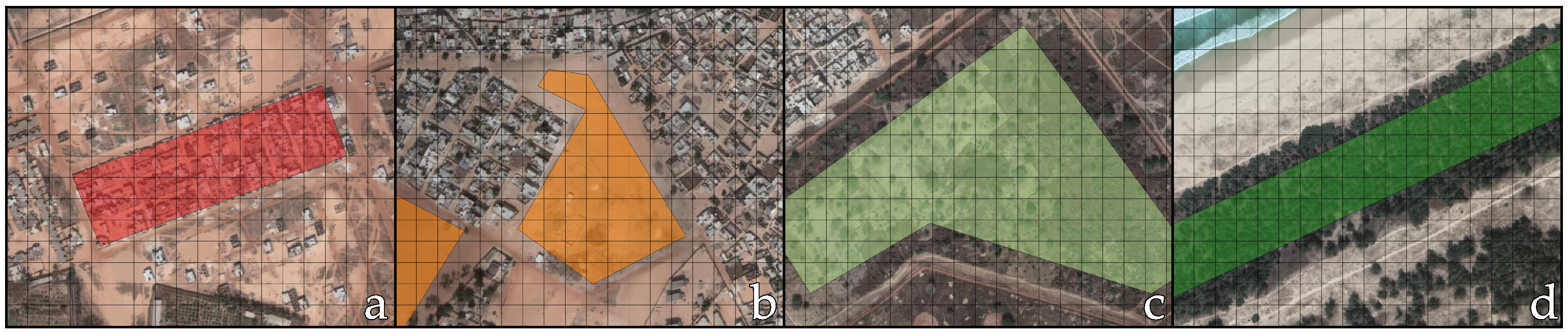
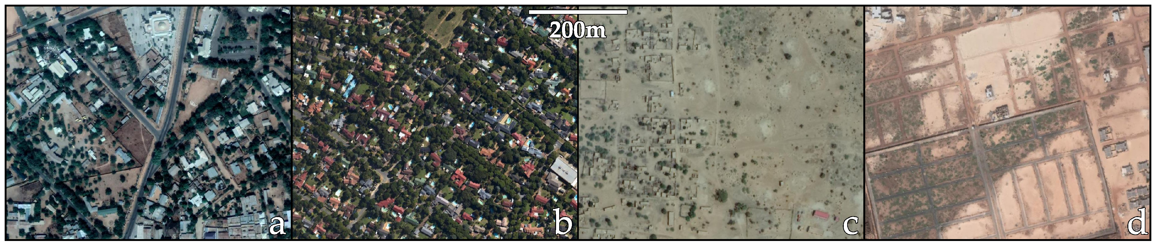
Reference samples for four land cover classes are collected using very high spatial resolution (VHSR) imagery from Google Earth (GE): built-up, bare soil, low vegetation (sparse vegetation, farms) and high vegetation (forests). The history slider of the GE interface has been used to ensure that the acquisition dates of the images are in a one-year range of the corresponding Landsat scenes. Even if our classification problem is binary (built-up vs. non-built-up), the collection of reference samples for specific land covers was preferred to ensure the spectral representativeness of the non-built-up landscape. As shown in Figure 1, samples were collected as polygons to include the inherent spectral heterogeneity of urban land covers. Reference built-up areas deliberately included mixed pixels provided that they contain at least 20% of built-up.
In total, more than 2400 polygons were digitized, corresponding to more than 180,000 pixels after rasterization. In the context of our case study, reference samples were used for: (1) assessing the quality of the training samples extracted from OSM; (2) assessing the performance of the built-up classifications; and (3) producing a reference classification for comparison purposes.
2.4. OpenStreetMap
OSM data were acquired in January 2018 using the Overpass API (http://overpass-api.de). Four different objects were collected from the database: (1) highway polylines (the road network); (2) building polygons (the building footprints); (3) the landuse, leisure, and natural polygons (potentially non-built-up objects); and (4) natural=water polygons (the water bodies). Complex geometries such as polygons with holes were not considered to simplify the processing.
As previously stated, spatial contribution patterns of OSM are not homogeneous. The evolution of OSM data availability for each type of object for each case study is shown in Figure 2. The trends observed at the continental scale are confirmed in the context of our case studies. As suggested by its name, OSM was initially focused on street mapping. Street mapping appears as a continuous effort that leads to a regular increase of the number of roads in the database. Later, contributors started to integrate building footprints, points of interest, or land use and land cover features. As a result, the number of building footprints, natural and land use polygons more than doubled between 2016 and 2018. These trends suggest that OSM can now support large-scaled supervised classification in developing regions. They also reveal that an increasing amount of data will be available in the near future.
2.5. Training Samples
2.5.1. Built-Up Training Samples
In the OSM database, the building key is used to mark an area as a building. When they are available, the building footprints are the perfect candidates for built-up training samples collection thanks to their unambiguous spatial definition. However, as shown in Figure 3, they are not consistently available among the cities. Highly populated urban areas such as Nairobi, Dakar or Johannesburg contain more than 1000 hectares of building footprints, whereas smaller cities such as Katsina and Gao only contain a few hectares, thus reducing the representativeness of the full built-up spectral signature. Such data availability issue implies that additional samples must be collected from another data source. Figure 3 also reveals that the typical building footprint does not cover more than 15% of the surface of a Landsat pixel. It means that, when going from the vector space to the 30 m raster space of our analysis, the geographic object is not the building footprint anymore but the percentage of the pixel which is effectively covered by any footprint. As a result, the decision to include or exclude a pixel from the built-up training samples relies on a binary threshold, under the assumption that, the higher the threshold, the lower the risk is to include mixed pixels.
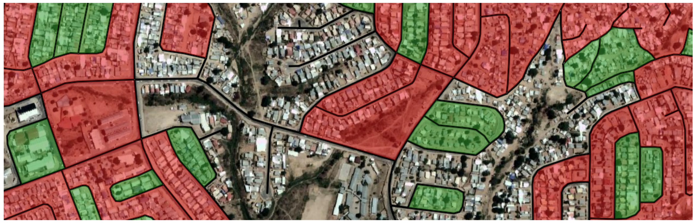
As previously stated, OSM building footprints are not a sufficient data source to collect built-up training samples because of inconsistencies in data availability among cities. The road network remains the most exhaustive feature in OSM: even the smallest cities among our case studies contain hundreds of kilometers of roads, and new streets are being mapped each month. As illustrated in Figure 4, built-up information can be derived from these road networks using the concept of urban blocks, defined as the polygons shaped by the intersection of the roads. To focus on residential blocks, only roads tagged as residential, tertiary, living_street, unclassified or with the generalist road value were used. Major roads such as highways, express ways or national roads were avoided, as well as service roads, tracks, and paths. In the case of Katsina and Gao, for which the building footprints did not provide a sufficient amount of built-up training samples, the process resulted in the availability of more than 1000 blocks. One assumption can be made regarding the reliability of such geographic objects to collect more built-up training samples: large blocks have a higher probability of containing mixed pixels or non-built-up areas.
2.5.2. Non-Built-Up Training Samples
Because of the focus of the OSM database on the urban objects, the extraction of non-built-up samples was less straightforward than the extraction of built-up samples. The OSM database includes information on the physical materials at the surface of the earth according to: (1) the description of various bio-physical landscape features such as grasslands or forests with the natural key; (2) the primary usage for an area of land such as farms, or managed forests and grasslands with the landuse key; and (3) the mapping of specific leisure features such as parks or nature reserves with the leisure key. Such objects are not ensured to be non-built-up and must be filtered according to their assigned value. From the 105 available values in our case studies, the following 20 values were selected: sand, farmland, wetland, wood, park, forest, nature_reserve, golf_course, cemetery, sand, quarry, pitch, scree, meadow, orchard, grass, recreation_ground, grassland, garden, heath, bare_rock, beach and greenfield.
However, the availability of non-built objects was not consistent among the case studies. Antananarivo, Johannesburg, Kampala, or Nairobi contained more than 1000 non-built-up objects according to the previously stated definition. On the contrary, smaller cities such as Chimoio or Katsina benefited from less than 50 objects. Given the spectral and spatial heterogeneity of the non-built landscape which may consist of different types of soil and vegetation, a low amount of non-built-up objects may induce a lack of representativeness in the training dataset. However, a large amount of urban information is available through the road network or the digitized building footprints. In the case of low OSM data availability, this information allows for the discrimination of areas with a low probability of being built-up. The underlying assumption is that the areas which are distant from any urban object, such as roads or buildings, have a low probability of being built-up, thereby making potential candidates for being used as non-built-up training samples. Under the previous assumptions, we define the urban distance as the distance from any road or building:
2.5.3. Quality Assessment of Training Samples
To assess the quality of the training samples extracted from the OSM database, we measured the distance between their spectral signatures and those of the reference land cover polygons. The spectral signature of an object is the variation of its reflectance values according to the wavelength. In the six non-thermal Landsat bands, the spectral signature S of an object can be defined as:
with being the mean pixel value of the object for the band n. Therefore, the euclidean spectral distance d between two objects x and y can be defined as:
More specifically, the optimal value of four parameters was investigated: (1) the minimum coverage threshold for the building footprints; (2) the maximum surface threshold for the urban blocks; (3) the accepted OSM tags for non-built-up objects; and (4) the minimum distance threshold for random selection of supplementary non-built-up samples from the urban distance raster.
2.6. Classification
Relying on crowd-sourced geographic information to automatically generate a training dataset implies that the resulting sample will be more noisy compared to a manual sampling strategy. Therefore, a larger amount of samples may be required to compensate the mislabeled points and the lack of representativeness. Consequently, the binary classification task (built-up vs. non-built) was performed using the Random Forest (RF) classifier, which has been shown to be computationally efficient and relatively robust to outliers and noisy training data [36,37]. The implementation was based on a set of Python libraries, including: NumPy [38] and SciPy [39] for scientific computing, Rasterio [40] for raster processing, Shapely [41] and Geopandas for vector analysis, and Scikit-learn [42] for machine learning. The code used to support the study is available on Github https://github.com/yannforget/builtup-classification-osm.
To remove errors and ambiguities caused by variations in acquisition conditions, the eight input Landsat bands were transformed to a Normalized Difference Spectral Vector (NDSV) [43] before the classification. The NDSV is a combination of all normalized spectral indices, as defined in Equations (4) and (5). In the case of Landsat, this leads to a vector of 28 normalized spectral indices.
To assess the ability of OSM for training supervised built-up classification, a comparative approach was adopted. Three distinct classifications were carried out using different training datasets, as described in Table 3. A reference classification () was performed using the reference land cover polygons as training samples to assess the relative performance of OSM-based approaches. In this case, reference polygons were randomly split between a training and a testing dataset of equal sizes. The procedure was repeated 20 times and the validation metrics were averaged. Training samples of the two other classifications ( and ) were exclusively extracted from OSM. The first one used first-order features from OSM: building footprints as built-up samples, and land use, natural and leisure polygons as non-built-up samples. The second one was designed to tackle the OSM data availability issue which may be encountered in less populated urban areas. It used second-order features derived from first-order objects such as urban blocks and urban distance.
In all three cases, RF parameters were set according to the recommendations of the literature [36,37]. RF decision tree ensembles were constructed with 100 trees, and the maximum number of features per tree was set to the square root of the total number of features. Imbalance issues between built-up and non-built-up training datasets sizes were tackled by over-sampling the minority class [44]. Additionally, fixed random seeds were set to ensure the reproducibility of the analysis.
2.7. Validation
Classification performances were assessed using the manually digitized reference land cover polygons as a testing dataset. Three validation metrics were computed: F1-score, precision and recall. The metrics were computed for the three classifications, as well as for two existing Landsat-based urban maps: the GHSL and the HBASE datasets.
3. Results and Discussion
3.1. Built-Up Training Samples
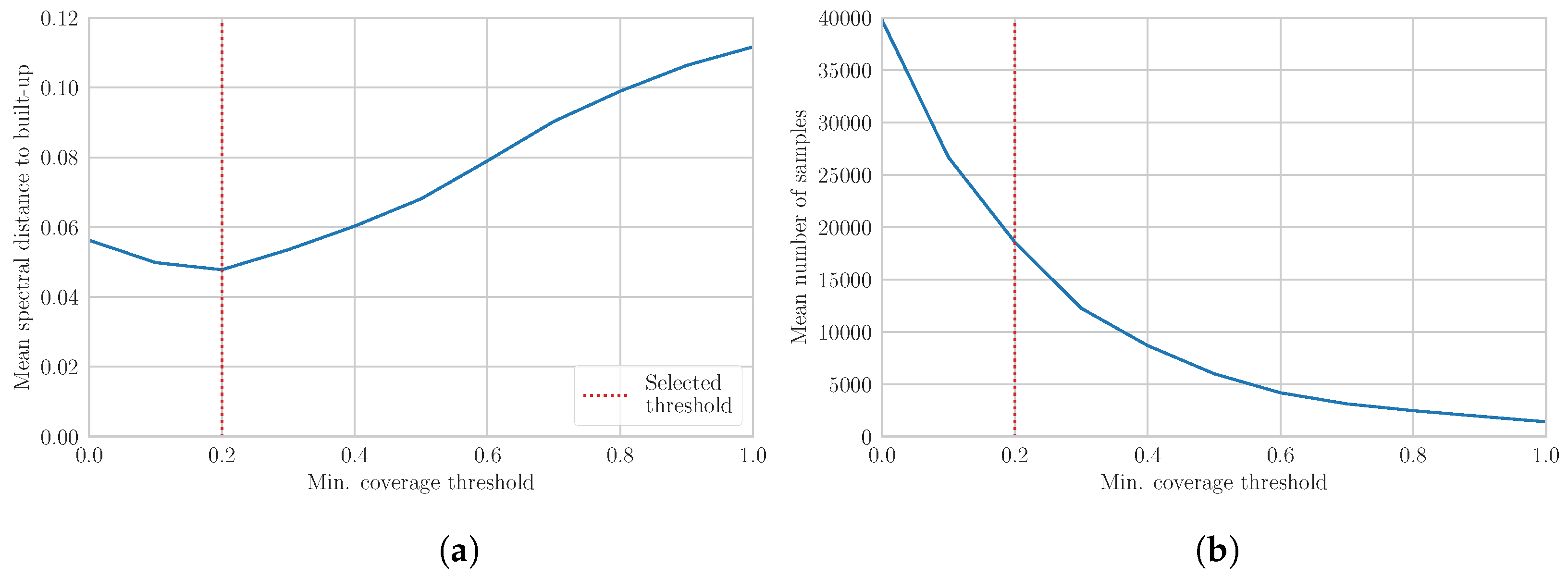
The extraction of built-up training samples from the OSM building footprints required the selection of a minimum coverage threshold. The impact of this threshold has been assessed by measuring the spectral distance of the resulting samples to the reference built-up samples. As shown in Figure 5a, the assumption that increasing the threshold would minimize the spectral distance to the reference built-up is not verified. Indeed, the highest spectral distances are reached when only fully covered pixels are selected. As shown in Figure 5b, the optimal threshold appears to be reached when a minimum of 20,000 samples are available. This reveals the importance of maximizing the representativeness of the sample by ensuring that a sufficient amount of samples is available. Furthermore, given the non-exhaustive nature of the OSM database, a pixel that contains a building footprint of any size have a high probability to contain additional unmapped built-up structures. However, low threshold values (between 0 and 0.2) appear to effectively increase the spectral similarity with the reference built-up samples by eliminating pixels covered by small and isolated buildings. Overall, a minimum coverage threshold of 0.2 appears to maximize both samples quality and quantity.
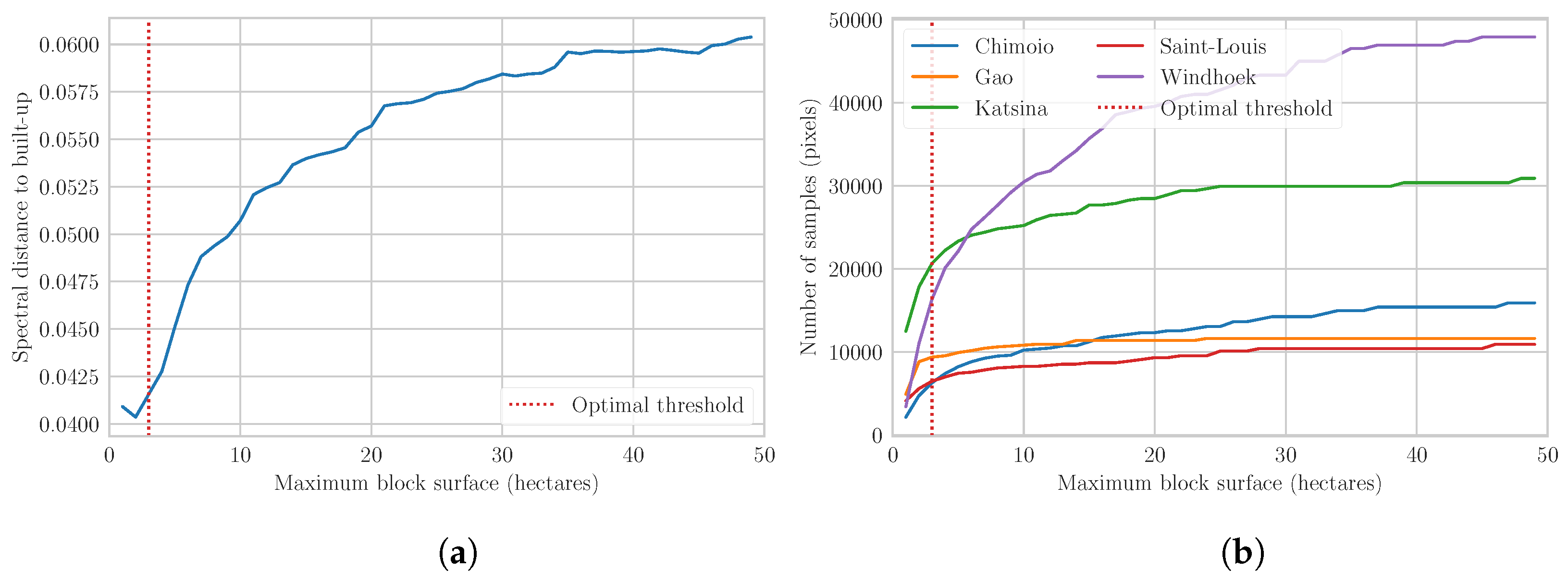
Urban blocks enabled the collection of built-up training samples where buildings footprints were lacking. Figure 6 shows the impact of the maximum surface threshold on both samples quality and quantity. As expected, excluding large blocks increases the spectral similarity with the reference built-up samples by avoiding highly mixed pixels and bare lands. The highest similarity is reached when only including the blocks with a surface lower than 1 ha. However, this conservative threshold dramatically reduces the sample size in small urban agglomerations such as Katsina, Gao, or Saint-Louis. Therefore, a maximum surface threshold of 3 ha was selected to ensure a sufficient amount of samples while minimizing the spectral distance to the reference built-up samples.
3.2. Non-Built-Up Training Samples
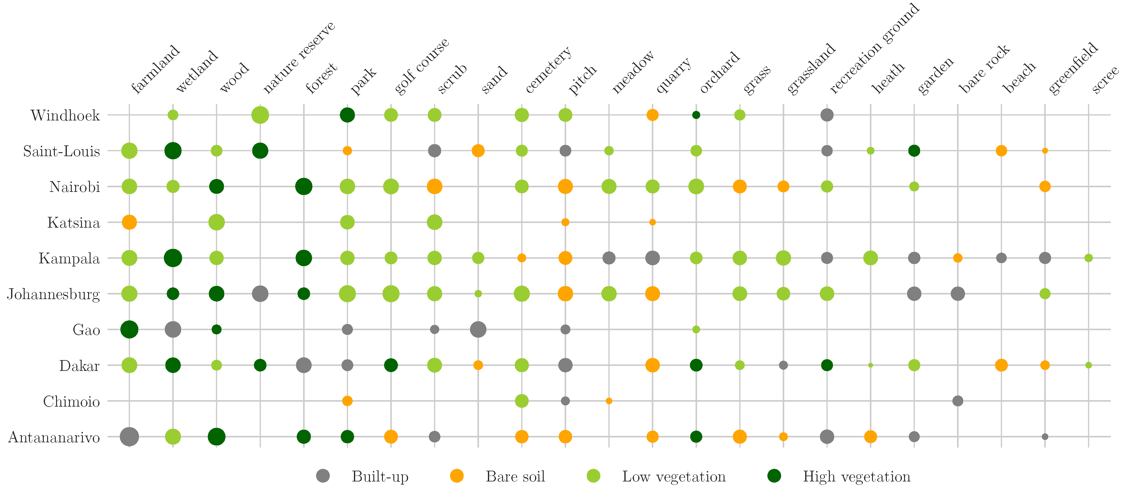
The non-built-up landscape is spectrally complex due to its irregular spatial patterns and the variations of soils and vegetation types. Figure 7 shows the most similar land cover of each OSM non-built-up tag in terms of spectral distance. The analysis reveals the spectral variability of OSM non-built-up objects across the case studies. Urban features such as garden, recreation_ground, pitch or park can have a spectral signature closer to built-up than to bare soil or lowly vegetated areas. The small surface covered by these features can lead to a high proportion of mixed pixels. Additionally, their urban nature makes highly probable the presence of human-constructed elements. On the contrary, natural features such as orchard, meadow, forest or wood are more consistently close to the spectral signature of vegetated areas. Generally, most of the features providing bare soil samples may be confused with built-up areas because of their urban nature (pitch) or their spectral similarity (beach). However, the decision boundary between built-up and bare soil pixels being the most prone to errors in urban areas, we choose to not exclude them in order to maximize the representativeness. Overall, these inconsistencies also highlight the fact that a supervised multi-class land cover classification based on OSM would be difficult to set up as of today.
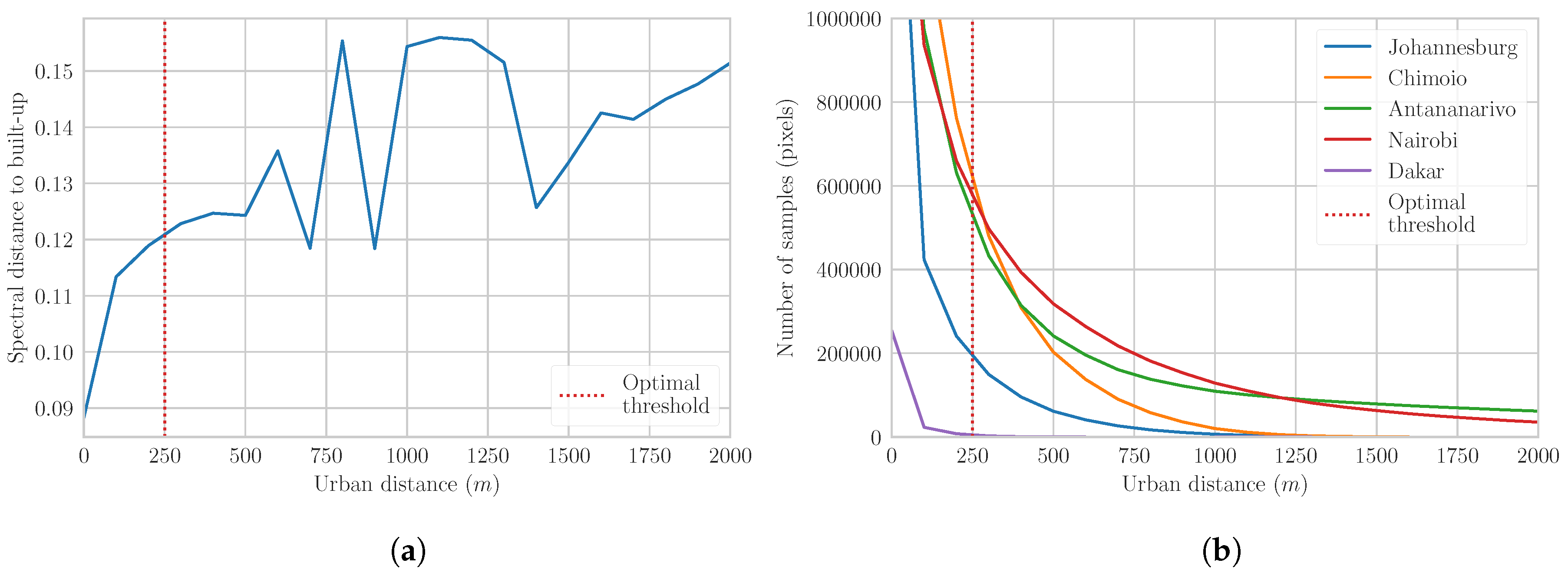
In case studies where OSM non-built-up objects were not sufficiently available, an urban distance raster was used to randomly collect supplementary training samples in remote areas. Figure 8 shows the relationship between the remoteness and the spectral distance to the reference built-up samples. As expected, the spectral distance increases with the urban distance. However, the spectral variations become inconsistent and are mainly caused by changes in the non-built-up landscape (e.g., forests, mountains, or bare lands). In highly urbanized agglomerations such as Johannesburg or Dakar, the road network covers the whole area of interest, leading to a very low amount of remote pixels. Consequently, a minimum distance threshold of 250 m was used.
3.3. GHSL and HBASE Assessment
The assessment metrics for the GHSL and HBASE datasets in the context of our case studies are shown in Table 4. They are provided as an indication of their relevance in the context of our case studies and our definition of a built-up area. They also reveal which case studies may be problematic for an automated built-up mapping method. For example, the arid urban area of Gao suffers from low recall scores because of the spectral confusion that occurs between the buildings materials and the bare surroundings areas. This leads to the misclassification of large built-up areas as bare lands. To a lesser extent, the semi-arid urban areas of Saint-Louis, Windhoek, and Katsina present the same issue. On the contrary, subtropical urban areas such as Antananarivo or Chimoio are characterized by an abundant vegetation in the urban mosaic. Thus, high rates of misclassifications are observed in the peripheral areas where built-up is less dense. A similar phenomenon is also noticed in the richest residential districts of Johannesburg. Overall, both datasets reach a mean F1-score of 0.82 when excluding Gao.
3.4. Classification Results
Assessment metrics of the three classification schemes are presented in Table 5. The reference classification, which has been trained with manually digitized samples, reached a mean F1-score of 0.92 and a minimum of 0.84 in Gao. Such results suggest that high classification performances can be achieved in most of the case studies provided that the training dataset is sufficiently large and representative. The first OSM-based classification scheme () made use of first-order OSM objects: buildings footprints and objects associated with a non-built up tag. Therefore, a limited availability in either of the aforementioned objects was highly detrimental to the classification performance. Katsina, Windhoek, and Johannesburg suffered from a low availability in building footprints with, respectively, 110, 2636, and 6724 objects. This led to an unrepresentative built-up training sample consisting mainly of large administrative structures or isolated settlements. In Chimoio, more than 150,000 building footprints were available. However, only 12 non-built-up polygons have been extracted from the OSM database, all related to forested areas. As a result, the lack of information regarding the spectral characteristics of the heterogeneous non-built-up landscape did not enable the separation between built-up and bare areas. A similar issue was also encountered in Antananarivo, where most of the non-built-up training samples were located in natural reserves and forests.
The second OSM-based classification scheme () was designed to tackle the aforementioned issues by deriving second-order features from the road network. The addition of built-up and non-built-up training samples collected from urban blocks and remote areas solved the data availability and representativeness issues in all the case studies, leading to better scores in 9 out of 10 cases. Overall, reached scores that were comparable to those of the reference classification. More specifically, had the highest recall scores, suggesting that the model was more successful in the detection of isolated, informal or peripheral settlements. Additionally, the use of larger training datasets (from 30,000 to 500,000 samples per case study) led to higher consistencies in the classification performance with a standard deviation of 0.02.
With , three case studies still had recall scores lower than 0.9: Gao, Johannesburg and Katsina. This suggests that the model did not effectively detect built-up in some areas. Figure 9 shows some examples of such areas. In Katsina, higher rates of misclassifications were observed in the northeast part of the city, where urban vegetation was denser that in other parts of the agglomeration. Furthermore, because of a less dense road network and the unavailability of building footprints, no training samples were available in this area. Likewise, the richest neighborhoods in Johannesburg are characterized by isolated buildings in a denser urban vegetation, leading to a higher rate of misclassification. In Gao, errors were mainly caused by the spectral confusion which occurred between built-up and bare soil areas. The phenomenon was exacerbated by the arid climate and the buildings materials made off nearby natural resources.
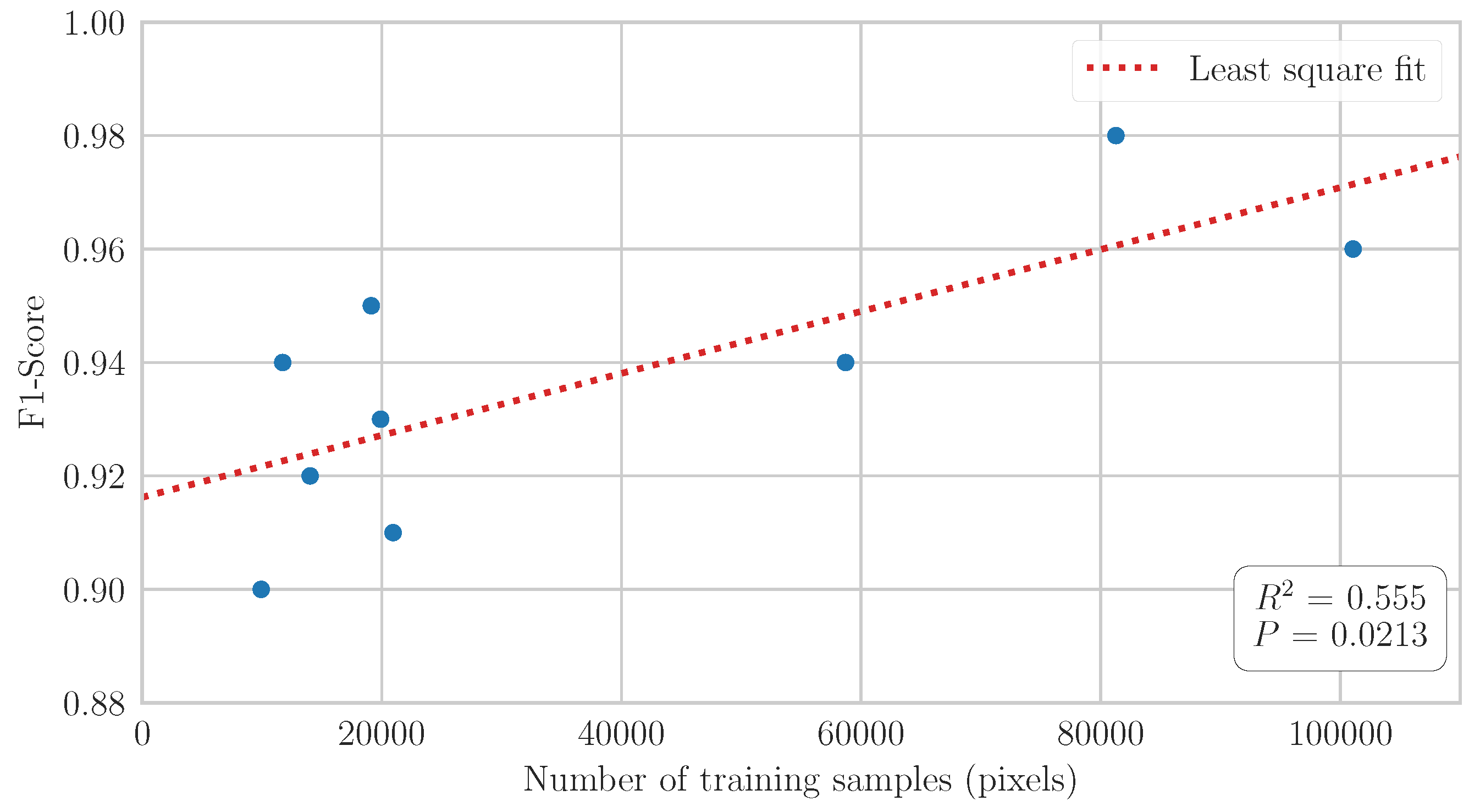
Generally, as shown in Figure 10, the classification scores increased with the number of training samples. Because of the introduction of noise and mislabaled samples inherent to automated approaches, large training datasets were required to make sense of the heterogeneous spectral characteristics of the urban environment. Figure 10 suggests that between 10,000 and 20,000 samples are necessary to fit the classification model depending on the spectral complexity of the urban mosaic.
4. Conclusions
This study provided important insights regarding the automatic collection of training samples to support large-scaled or rapid supervised classification of built-up areas. The proposed method made use of the growing amount of information in the OSM database to automatically extract both built-up and non-built-up training samples. This automated approach can reach classification performances similar to manual sampling strategies, provided that a relevant set of pre-processing routines are applied. In some less populated urban areas, first-order urban features—such as building footprints—can be too scarce. The issue of data scarcity can be tackled by a spatial analysis of the road network to derive second-order features such as urban blocks or urban distance. The proposed approach reached a mean F1-score of 0.93 across our case studies, while the manual approach reached 0.92. Case studies located in arid climates suffer from higher misclassification rates because of the spectral confusion that occurs between the building materials and the bare soil. The issue could be addressed by using a higher resolution imagery such as Sentinel-2. Likewise, the use of Synthetic Aperture Radar (SAR) to extract textural features should lead to a better separation between built-up and bare soil.
Automatically generated training datasets contain more noise than manually collected samples. Additionally, the reliance on crowd-sourced geographic information introduces its own share of errors and inconsistencies. Previous studies have shown that the RF classifier can handle up to 20% noise in the training dataset, provided that the sample size is large enough [37]. Overall, these previous findings are confirmed by our results. In our case studies, maximizing the size of the training dataset was more advantageous than minimizing the noise.
Land use and land cover mapping in the OSM community is a relatively new phenomenon, especially in developing regions. In fact, 77% of the building footprints and 50% of the land use polygons used in this study have been mapped after January 2016. The growing amount of available data suggests that the proposed approach will provide better results in following years. More importantly, the mapping of land use and natural elements could enable multi-class supervised land cover classifications in the near future.
Author Contributions
Conceptualization, Y.F., C.L. and M.G.; Data curation, Y.F.; Formal analysis, Y.F.; Funding acquisition, C.L. and M.G.; Investigation, Y.F.; Methodology, Y.F.; Project administration, C.L. and M.G.; Resources, M.G.; Software, Y.F.; Supervision, C.L. and M.G.; Validation, Y.F., C.L. and M.G.; Visualization, Y.F.; Writing—original draft, Y.F.; and Writing—review and editing, Y.F., C.L. and M.G.
Funding
This research was funded by the Belgian Science Policy Office and is part of the research project SR/00/304 MAUPP (Modelling and Forecasting African Urban Population Patterns for Vulnerability and Health Assessments).
Conflicts of Interest
The authors declare no conflict of interest.
References
- UN-Habitat. The State of African Cities, 2014: Re-Imagining Sustainable Urban Transitions; UN-Habitat: Nairobi, Kenya, 2014. [Google Scholar]
- Grimm, N.B.; Faeth, S.H.; Golubiewski, N.E.; Redman, C.L.; Wu, J.; Bai, X.; Briggs, J.M. Global Change and the Ecology of Cities. Science 2008, 319, 756–760. [Google Scholar] [CrossRef] [PubMed]
- Dye, C. Health and Urban Living. Science 2008, 319, 766–769. [Google Scholar] [CrossRef] [PubMed]
- Wentz, E.; Anderson, S.; Fragkias, M.; Netzband, M.; Mesev, V.; Myint, S.; Quattrochi, D.; Rahman, A.; Seto, K. Supporting Global Environmental Change Research: A Review of Trends and Knowledge Gaps in Urban Remote Sensing. Remote Sens. 2014, 6, 3879–3905. [Google Scholar] [CrossRef] [Green Version]
- Arino, O.; Leroy, M.; Ranera, F.; Gross, D.; Bicheron, P.; Nino, F.; Brockman, C.; Defourny, P.; Vancutsem, C.; Achard, F. Globcover-a Global Land Cover Service with MERIS. In Proceedings of the ENVISAT Symposium, Montreux, Switzerland, 23–27 April 2007; pp. 23–27. [Google Scholar]
- Schneider, A.; Friedl, M.A.; Potere, D. A New Map of Global Urban Extent from MODIS Satellite Data. Environ. Res. Lett. 2009, 4. [Google Scholar] [CrossRef]
- Wulder, M.A.; White, J.C.; Goward, S.N.; Masek, J.G.; Irons, J.R.; Herold, M.; Cohen, W.B.; Loveland, T.R.; Woodcock, C.E. Landsat Continuity: Issues and Opportunities for Land Cover Monitoring. Remote Sens. Environ. 2008, 112, 955–969. [Google Scholar] [CrossRef]
- Pesaresi, M.; Ehrlich, D.; Ferri, S.; Florczyk, A.J.; Freire, S.; Halkia, M.; Julea, A.; Kemper, T.; Soille, P.; Syrris, V. Operating Procedure for the Production of the Global Human Settlement Layer from Landsat Data of the Epochs 1975, 1990, 2000, and 2014; Technical Report; Joint Research Centre, European Commission: Brussels, Belgium; Luxembourg, 2016. [Google Scholar]
- Chen, J.; Chen, J.; Liao, A.; Cao, X.; Chen, L.; Chen, X.; He, C.; Han, G.; Peng, S.; Lu, M.; Zhang, W.; Tong, X.; Mills, J. Global Land Cover Mapping at 30m Resolution: A POK-Based Operational Approach. ISPRS J. Photogramm. Remote Sens. 2015, 103, 7–27. [Google Scholar] [CrossRef]
- Wang, P.; Huang, C.; Brown de Colstoun, E.C.; Tilton, J.C.; Tan, B. Human Built-up And Settlement Extent (HBASE) Dataset From Landsat. 2017. Available online: https://doi.org/10.7927/H4DN434S (accessed on 1 June 2018).
- Herold, M.; Roberts, D.A.; Gardner, M.E.; Dennison, P.E. Spectrometry for Urban Area Remote Sensing—Development and Analysis of a Spectral Library from 350 to 2400 Nm. Remote Sens. Environ. 2004, 91, 304–319. [Google Scholar] [CrossRef]
- Small, C. A Global Analysis of Urban Reflectance. Int. J. Remote Sens. 2005, 26, 661–681. [Google Scholar] [CrossRef]
- Gamba, P.; Herold, M. Global Mapping of Human Settlement: Experiences, Datasets, and Prospects; Taylor & Francis Series in Remote Sensing Applications; CRC Press: Boca Raton, FL, USA, 2009. [Google Scholar]
- Li, M. A Review of Remote Sensing Image Classification Techniques: The Role of Spatio-Contextual Information. Eur. J. Remote Sens. 2014, 389–411. [Google Scholar] [CrossRef]
- Belgiu, M.; Drăguţ, L. Random Forest in Remote Sensing: A Review of Applications and Future Directions. ISPRS J. Photogramm. Remote Sens. 2016, 114, 24–31. [Google Scholar] [CrossRef]
- Potere, D.; Schneider, A.; Angel, S.; Civco, D. Mapping Urban Areas on a Global Scale: Which of the Eight Maps Now Available Is More Accurate? Int. J. Remote Sens. 2009, 30, 6531–6558. [Google Scholar] [CrossRef]
- Trianni, G.; Lisini, G.; Angiuli, E.; Moreno, E.A.; Dondi, P.; Gaggia, A.; Gamba, P. Scaling up to National/Regional Urban Extent Mapping Using Landsat Data. IEEE J. Sel. Top. Appl. Earth Observ. Remote Sens. 2015, 8, 3710–3719. [Google Scholar] [CrossRef]
- Goodchild, M.F. Citizens as Sensors: The World of Volunteered Geography. GeoJournal 2007, 69, 211–221. [Google Scholar] [CrossRef]
- Haklay, M.; Weber, P. OpenStreetMap: User-Generated Street Maps. IEEE Pervas. Comput. 2008, 7, 12–18. [Google Scholar] [CrossRef] [Green Version]
- Mooney, P.; Minghini, M. A Review of OpenStreetMap Data. In Mapping and the Citizen Sensor; Ubiquity Press: London, UK, 2017; pp. 37–59. [Google Scholar] [Green Version]
- Estima, J.; Painho, M. Exploratory Analysis of OpenStreetMap for Land Use Classification. In Proceedings of the Second ACM SIGSPATIAL International Workshop on Crowdsourced and Volunteered Geographic Information, Orlando, FL, USA, 5 November 2013; ACM Press: New York, NY, USA, 2013; pp. 39–46. [Google Scholar] [CrossRef]
- Estima, J.; Painho, M. Investigating the Potential of OpenStreetMap for Land Use/Land Cover Production: A Case Study for Continental Portugal. In OpenStreetMap in GIScience; Jokar Arsanjani, J., Zipf, A., Mooney, P., Helbich, M., Eds.; Springer International Publishing: Cham, Switzerland, 2015; pp. 273–293. [Google Scholar]
- Jokar Arsanjani, J.; Helbich, M.; Bakillah, M.; Hagenauer, J.; Zipf, A. Toward Mapping Land-Use Patterns from Volunteered Geographic Information. Int. J. Geogr. Inf. Sci. 2013, 27, 2264–2278. [Google Scholar] [CrossRef]
- Fonte, C.; Minghini, M.; Patriarca, J.; Antoniou, V.; See, L.; Skopeliti, A. Generating Up-to-Date and Detailed Land Use and Land Cover Maps Using OpenStreetMap and GlobeLand30. ISPRS Int. J. Geo-Inf. 2017, 6, 125. [Google Scholar] [CrossRef]
- Schultz, M.; Voss, J.; Auer, M.; Carter, S.; Zipf, A. Open Land Cover from OpenStreetMap and Remote Sensing. Int. J. Appl. Earth Observ. Geoinf. 2017, 63, 206–213. [Google Scholar] [CrossRef]
- Yang, D.; Fu, C.S.; Smith, A.C.; Yu, Q. Open Land-Use Map: A Regional Land-Use Mapping Strategy for Incorporating OpenStreetMap with Earth Observations. Geo-Spat. Inf. Sci. 2017, 20, 269–281. [Google Scholar] [CrossRef]
- Coleman, D.J.; Georgiadou, Y.; Labonte, J. Volunteered Geographic Information: The Nature and Motivation of Produsers. Int. J. Spat. Data Infrastruct. Res. 2009, 4, 27. [Google Scholar]
- Juhász, L.; Hochmair, H. OSM Data Import as an Outreach Tool to Trigger Community Growth? A Case Study in Miami. ISPRS Int. J. Geo-Inf. 2018, 7, 113. [Google Scholar] [CrossRef]
- Zhang, C.; Chen, Y.; Lu, D. Mapping the Land-Cover Distribution in Arid and Semiarid Urban Landscapes with Landsat Thematic Mapper Imagery. Int. J. Remote Sens. 2015, 36, 4483–4500. [Google Scholar] [CrossRef]
- Li, H.; Wang, C.; Zhong, C.; Su, A.; Xiong, C.; Wang, J.; Liu, J. Mapping Urban Bare Land Automatically from Landsat Imagery with a Simple Index. Remote Sens. 2017, 9, 249. [Google Scholar] [CrossRef]
- Kottek, M.; Grieser, J.; Beck, C.; Rudolf, B.; Rubel, F. World Map of the Köppen-Geiger Climate Classification Updated. Meteorol. Z. 2006, 15, 259–263. [Google Scholar] [CrossRef]
- Linard, C.; Gilbert, M.; Snow, R.W.; Noor, A.M.; Tatem, A.J. Population Distribution, Settlement Patterns and Accessibility across Africa in 2010. PLoS ONE 2012, 7, e31743. [Google Scholar] [CrossRef] [PubMed]
- Vermote, E.; Justice, C.; Claverie, M.; Franch, B. Preliminary Analysis of the Performance of the Landsat 8/OLI Land Surface Reflectance Product. Remote Sens. Environ. 2016, 185, 46–56. [Google Scholar] [CrossRef]
- Zhu, Z.; Woodcock, C.E. Object-Based Cloud and Cloud Shadow Detection in Landsat Imagery. Remote Sens. Environ. 2012, 118, 83–94. [Google Scholar] [CrossRef]
- Zhu, Z.; Wang, S.; Woodcock, C.E. Improvement and Expansion of the Fmask Algorithm: Cloud, Cloud Shadow, and Snow Detection for Landsats 4–7, 8, and Sentinel 2 Images. Remote Sens. Environ. 2015, 159, 269–277. [Google Scholar] [CrossRef]
- Rodriguez-Galiano, V.; Ghimire, B.; Rogan, J.; Chica-Olmo, M.; Rigol-Sanchez, J. An Assessment of the Effectiveness of a Random Forest Classifier for Land-Cover Classification. ISPRS J. Photogramm. Remote Sens. 2012, 67, 93–104. [Google Scholar] [CrossRef]
- Mellor, A.; Boukir, S.; Haywood, A.; Jones, S. Exploring Issues of Training Data Imbalance and Mislabelling on Random Forest Performance for Large Area Land Cover Classification Using the Ensemble Margin. ISPRS J. Photogramm. Remote Sens. 2015, 105, 155–168. [Google Scholar] [CrossRef]
- Oliphant, T.E. Guide to NumPy; Continuum Press: Austin, TX, USA, 2015. [Google Scholar]
- Jones, E.; Oliphant, E.; Peterson, P. SciPy: Open Source Scientific Tools for Python. 2001. Available online: scipy.org (accessed on 1 June 2018).
- Gillies, S.; Perry, M.; Wurster, K.; Ward, B.; Solvsteen, J.; Talbert, C.; McBride, J.; Seglem, E.; Sarago, V.; Fitzsimmons, S.; et al. Rasterio: Geospatial Raster I/O for Python Programmers. 2013. Available online: github.com/mapbox/rasterio (accessed on 1 June 2018).
- Gillies, S.; Tonnhofer, O.; Arnott, J.; Toews, M.; Wasserman, J.; Bierbaum, A.; Adair, A.; Shonberger, J.; Elson, P.; Butler, H.; et al. Shapely: Manipulation and analysis of geometric objects. 2007. Available online: github.com/Toblerity/Shapely (accessed on 1 June 2018).
- Pedregosa, F.; Varoquaux, G.; Gramfort, A.; Michel, V.; Thirion, B.; Grisel, O.; Blondel, M.; Prettenhofer, P.; Weiss, R.; Dubourg, V. Scikit-Learn: Machine Learning in Python. J. Mach. Learn. Res. 2011, 12, 2825–2830. [Google Scholar]
- Angiuli, E.; Trianni, G. Urban Mapping in Landsat Images Based on Normalized Difference Spectral Vector. IEEE Geosci. Remote Sens. Lett. 2014, 11, 661–665. [Google Scholar] [CrossRef]
- Lemaître, G.; Nogueira, F.; Aridas, C.K. Imbalanced-Learn: A Python Toolbox to Tackle the Curse of Imbalanced Datasets in Machine Learning. J. Mach. Learn. Res. 2017, 18, 1–5. [Google Scholar]
Figure 1.
Examples of digitized samples in Dakar, Senegal: (a) Built-up; (b) Bare soil; (c) Low vegetation; and (d) High vegetation. The grid corresponds to the 30 meters Landsat pixels. Satellite imagery courtesy of Google Earth.
Figure 1.
Examples of digitized samples in Dakar, Senegal: (a) Built-up; (b) Bare soil; (c) Low vegetation; and (d) High vegetation. The grid corresponds to the 30 meters Landsat pixels. Satellite imagery courtesy of Google Earth.

Figure 2.
Evolution of OSM data availability in our case studies between 2011 and 2018.

Figure 3.
Availability and median surface of building footprints in each case study.

Figure 4.
Urban blocks extracted from the OSM road network in Windhoek, Namibia (transparent: surface greater than 10 ha; red: surface greater than 1 ha; green: surface lower than 1 ha). Satellite imagery courtesy of Google.
Figure 4.
Urban blocks extracted from the OSM road network in Windhoek, Namibia (transparent: surface greater than 10 ha; red: surface greater than 1 ha; green: surface lower than 1 ha). Satellite imagery courtesy of Google.

Figure 5.
Quality and quantity of built-up training samples extracted from OSM building footprints according to the minimum coverage threshold in the 10 case studies: (a) mean spectral distance to the reference built-up samples; and (b) mean number of samples (in pixels).
Figure 5.
Quality and quantity of built-up training samples extracted from OSM building footprints according to the minimum coverage threshold in the 10 case studies: (a) mean spectral distance to the reference built-up samples; and (b) mean number of samples (in pixels).

Figure 6.
Quality and quantity of built-up training samples extracted from OSM urban blocks according to maximum surface threshold in the 10 case studies: (a) mean spectral distance to the reference built-up samples; and (b) number of samples (in pixels) in the five case studies with the lowest data availability.

Figure 7.
Most similar land cover of each OSM non-built-up object according to its tag. Circles are logarithmically proportional to the number of pixels available.
Figure 7.
Most similar land cover of each OSM non-built-up object according to its tag. Circles are logarithmically proportional to the number of pixels available.

Figure 8.
Quality and quantity of non-built-up training samples extracted from the OSM-based urban distance raster: (a) mean spectral distance to the reference built-up samples according to the urban distance; and (b) number of samples (in pixels) in the five case studies with the lowest sample availability.

Figure 9.
Areas with high rates of misclassifications in: (a) Katsina; (b) Johannesburg; (c) Gao; and (d) Dakar. Satellite imagery courtesy of Google Earth.
Figure 9.
Areas with high rates of misclassifications in: (a) Katsina; (b) Johannesburg; (c) Gao; and (d) Dakar. Satellite imagery courtesy of Google Earth.

Figure 10.
Relationship between the number of training samples and the classification F1-score (the outlier Johannesburg is excluded from the graph).
Figure 10.
Relationship between the number of training samples and the classification F1-score (the outlier Johannesburg is excluded from the graph).


Table 1.
Environmental and demographic characteristics of the case studies. Climate zones are identified according to the Köppen–Geiger classification [31]. Population numbers are estimated according to the AfriPop/WorldPop dataset [32] for the AOI of each case study.
| City | Country | Climate | Population |
|---|---|---|---|
| Antananarivo | Madagascar | Subtropical highland | 2,452,000 |
| Chimoio | Mozambique | Humid subtropical | 462,000 |
| Dakar | Senegal | Hot semi-arid | 3,348,000 |
| Gao | Mali | Hot desert | 163,000 |
| Johannesburg | South Africa | Subtropical highland | 4,728,000 |
| Kampala | Uganda | Tropical rainforest | 3,511,000 |
| Katsina | Nigeria | Hot semi-arid | 1,032,000 |
| Nairobi | Kenya | Temperate oceanic | 5,080,000 |
| Saint-Louis | Senegal | Hot desert | 305,000 |
| Windhoek | Namibia | Hot semi-arid | 384,000 |
Table 2.
Product identifiers and acquisition dates of each Landsat scene.
| City | Landsat Product Identifier | Acquisition Date |
|---|---|---|
| Antananarivo | LC08_L1TP_159073_20150919_20170404_01_T1 | 2015–09–19 |
| Chimoio | LC08_L1TP_168073_20150529_20170408_01_T1 | 2015–05–29 |
| Dakar | LC08_L1TP_206050_20151217_20170331_01_T1 | 2015–12–07 |
| Gao | LC08_L1TP_194049_20160114_20170405_01_T1 | 2016–01–14 |
| Johannesburg | LC08_L1TP_170078_20150831_20170404_01_T1 | 2015–08–31 |
| Kampala | LC08_L1TP_171060_20160129_20170330_01_T1 | 2016–01–29 |
| Katsina | LC08_L1TP_189051_20160111_20170405_01_T1 | 2016–01–11 |
| Nairobi | LC08_L1TP_168061_20160124_20170330_01_T1 | 2016–01–24 |
| Saint-Louis | LC08_L1TP_205049_20161009_20170320_01_T1 | 2016–10–09 |
| Windhoek | LC08_L1TP_178076_20160114_20170405_01_T1 | 2016–01–14 |
Table 3.
Training samples data sources for each classification scheme.
| Built-Up | Non-Built-Up | |
|---|---|---|
| Reference built-up polygons | Reference non-built polygons | |
| Building footprints | Non-built features | |
| Building footprints & urban blocks | Non-built features & urban distance |
Table 4.
Assessment metrics of the GHSL and HBASE datasets. F1-scores lower than 0.80 are in red.
| GHSL | HBASE | |||||
|---|---|---|---|---|---|---|
| F1-Score | Precision | Recall | F1-Score | Precision | Recall | |
| Antananarivo | 0.83 | 0.82 | 0.83 | 0.79 | 0.67 | 0.96 |
| Chimoio | 0.47 | 0.98 | 0.31 | 0.82 | 0.94 | 0.73 |
| Dakar | 0.85 | 0.74 | 0.99 | 0.81 | 0.69 | 0.98 |
| Gao | 0.35 | 0.98 | 0.21 | 0.72 | 0.94 | 0.59 |
| Johannesburg | 0.92 | 0.86 | 0.99 | 0.90 | 0.82 | 0.99 |
| Kampala | 0.96 | 0.95 | 0.96 | 0.95 | 0.93 | 0.97 |
| Katsina | 0.90 | 0.92 | 0.88 | 0.64 | 0.76 | 0.56 |
| Nairobi | 0.84 | 0.96 | 0.75 | 0.88 | 0.81 | 0.97 |
| Saint Louis | 0.76 | 0.95 | 0.63 | 0.81 | 0.97 | 0.70 |
| Windhoek | 0.81 | 0.92 | 0.73 | 0.78 | 0.65 | 0.99 |
| Mean | 0.77 | 0.91 | 0.73 | 0.81 | 0.82 | 0.85 |
| Standard dev. | 0.20 | 0.08 | 0.28 | 0.09 | 0.12 | 0.18 |
Table 5.
Assessment metrics for the three classification schemes. F1-scores lower than 0.80 are in red.
Table 5.
Assessment metrics for the three classification schemes. F1-scores lower than 0.80 are in red.
| F1-Score | Precision | Recall | F1-Score | Precision | Recall | F1-Score | Precision | Recall | |
|---|---|---|---|---|---|---|---|---|---|
| Antananarivo | 0.78 | 0.99 | 0.65 | 0.93 | 0.91 | 0.96 | 0.92 | 0.97 | 0.87 |
| Chimoio | 0.77 | 0.63 | 0.97 | 0.92 | 0.90 | 0.95 | 0.85 | 0.93 | 0.79 |
| Dakar | 0.95 | 0.98 | 0.92 | 0.96 | 0.94 | 0.98 | 0.94 | 0.98 | 0.90 |
| Gao | 0.81 | 0.96 | 0.69 | 0.90 | 0.94 | 0.86 | 0.84 | 0.84 | 0.86 |
| Johannesburg | 0.60 | 0.98 | 0.43 | 0.92 | 0.99 | 0.86 | 0.96 | 0.98 | 0.94 |
| Kampala | 0.98 | 1.00 | 0.97 | 0.98 | 0.99 | 0.96 | 0.98 | 0.99 | 0.96 |
| Katsina | 0.20 | 0.84 | 0.11 | 0.91 | 0.95 | 0.87 | 0.94 | 0.99 | 0.90 |
| Nairobi | 0.91 | 0.94 | 0.89 | 0.94 | 0.97 | 0.92 | 0.93 | 0.97 | 0.89 |
| Saint-Louis | 0.95 | 0.98 | 0.93 | 0.94 | 0.92 | 0.96 | 0.92 | 0.98 | 0.88 |
| Windhoek | 0.68 | 0.98 | 0.52 | 0.95 | 0.93 | 0.98 | 0.93 | 0.96 | 0.90 |
| Mean | 0.76 | 0.93 | 0.71 | 0.94 | 0.95 | 0.93 | 0.92 | 0.96 | 0.89 |
| Standard dev. | 0.23 | 0.11 | 0.29 | 0.02 | 0.03 | 0.05 | 0.04 | 0.05 | 0.05 |
© 2018 by the authors. Licensee MDPI, Basel, Switzerland. This article is an open access article distributed under the terms and conditions of the Creative Commons Attribution (CC BY) license (http://creativecommons.org/licenses/by/4.0/).
Share and Cite
MDPI and ACS Style
Forget, Y.; Linard, C.; Gilbert, M. Supervised Classification of Built-Up Areas in Sub-Saharan African Cities Using Landsat Imagery and OpenStreetMap. Remote Sens. 2018, 10, 1145. https://doi.org/10.3390/rs10071145
AMA Style
Forget Y, Linard C, Gilbert M. Supervised Classification of Built-Up Areas in Sub-Saharan African Cities Using Landsat Imagery and OpenStreetMap. Remote Sensing. 2018; 10(7):1145. https://doi.org/10.3390/rs10071145
Chicago/Turabian StyleForget, Yann, Catherine Linard, and Marius Gilbert. 2018. "Supervised Classification of Built-Up Areas in Sub-Saharan African Cities Using Landsat Imagery and OpenStreetMap" Remote Sensing 10, no. 7: 1145. https://doi.org/10.3390/rs10071145
Note that from the first issue of 2016, this journal uses article numbers instead of page numbers. See further details here.