Individual Tree Crown Segmentation and Classification of 13 Tree Species Using Airborne Hyperspectral Data

Abstract

Knowledge of the distribution of tree species within a forest is key for multiple economic and ecological applications. This information is traditionally acquired through time-consuming and thereby expensive field work. Our study evaluates the suitability of a visible to near-infrared (VNIR) hyperspectral dataset with a spatial resolution of 0.4 m for the classification of 13 tree species (8 broadleaf, 5 coniferous) on an individual tree crown level in the UNESCO Biosphere Reserve ‘Wienerwald’, a temperate Austrian forest. The study also assesses the automation potential for the delineation of tree crowns using a mean shift segmentation algorithm in order to permit model application over large areas. Object-based Random Forest classification was carried out on variables that were derived from 699 manually delineated as well as automatically segmented reference trees. The models were trained separately for two strata: small and/or conifer stands and high broadleaf forests. The two strata were delineated beforehand using CHM-based tree height and NDVI. The predictor variables encompassed spectral reflectance, vegetation indices, textural metrics and principal components. After feature selection, the overall classification accuracy (OA) of the classification based on manual delineations of the 13 tree species was 91.7% (Cohen’s kappa (κ) = 0.909). The highest user’s and producer’s accuracies were most frequently obtained for Weymouth pine and Scots Pine, while European ash was most often associated with the lowest accuracies. The classification that was based on mean shift segmentation yielded similarly good results (OA = 89.4% κ = 0.883). Based on the automatically segmented trees, the Random Forest models were also applied to the whole study site (1050 ha). The resulting tree map of the study area confirmed a high abundance of European beech (58%) with smaller amounts of oak (6%) and Scots pine (5%). We conclude that highly accurate tree species classifications can be obtained from hyperspectral data covering the visible and near-infrared parts of the electromagnetic spectrum. Our results also indicate a high automation potential of the method, as the results from the automatically segmented tree crowns were similar to those that were obtained for the manually delineated tree crowns.

1. Introduction

The number of remote sensing papers focusing on tree species classification has increased substantially over the past few decades mainly due to a higher availability of multi- and hyperspectral data [1]. While forest managers and the timber industry have an obvious interest in data on timber resources [2], hyperspectral and LiDAR data can also be used for a variety of ecological applications [3]. Spatially detailed information on the distribution and the share of species facilitates, for example, (1) close-to-nature forest management [4], (2) the monitoring of invasive species [5] as well as (3) targeted conservation efforts [6]. While field assessments are the method of choice to acquire detailed information for small areas, it is not an option for large areas. Only remote sensing approaches have the potential to provide detailed information on large areas in a cost-efficient and reliable way.

The distinct spectral signature of a tree species relies on its structural, morphological and (bio-)chemical properties, e.g., water content and the amount of photosynthetic pigments [7,8,9,10]. Under comparable site conditions, trees of the same species, but of a different age or health state, may feature different spectral signatures [10,11,12,13,14,15], while the overall shape of the reflection curve is widely conserved across species borders [16]. As pointed out by Fassnacht et al. (2016), it is merely the amplitude of the peaks that is affected by the changes of the structural, morphological and chemical properties, and therefore discriminative power. In reality, however, the remotely recorded signal is rarely the pure signature of a tree. The observed spectral radiance is rather the mixture of signals from the tree itself—the useful signal—and the understory. Together with shading effects, the understory is the main perturbing factor for tree species discrimination. The strong effect of understory reflectance on the overall signal has been demonstrated both experimentally [17] as well as using physically based radiative transfer models [18].

Hyperspectral data in the optical range are well suited to capture subtle changes in the reflectance spectra of vegetation. Unlike multispectral data, data cubes that are derived from imaging spectrometers are characterized by many narrow, contiguous bands. These may span the electromagnetic spectrum from the visible to near-infrared until the short-wave infrared (SWIR) portion [19]. Some sensors are even capable of measuring detailed spectral properties in the thermal infrared [20]. Due to the narrowness and the high number of bands, meticulous spectral signatures can be determined [21]. The small band width decreases the risk that highly discriminative reflectance values of narrow stretches of the spectrum are drowned out. Fassnacht et al. (2016) report that in 13 reviewed studies, most parts of the spectrum were considered important at least once. This points to the need for using contiguous data with a high spectral resolution. However, with a narrowing band width, the signal-to-noise ratio decreases [19], which makes the application of smoothing and filtering techniques necessary. To cover very large areas, the currently very high costs of hyperspectral data also have to be considered [1,22].

A tree crown is a distinct object with a strong spectral variability and is often surrounded by cavities exposing shadows and forest floor. With the availability of (sub-)meter spatial resolution data it is therefore advisable to use object-based classification approaches [4,23]. In object-based classifications, pixels belonging to the same object are grouped and subsequently classified. The asset of object-based classification is that besides the spectral information also the shape or texture of an object can also be included in the analysis. This can become beneficial particularly for data with a high spatial resolution [24]. Reference tree polygons for model training can be manually delineated or generated using well established automated segmentation techniques such as watershed or region growing [25]. Automated approaches build on object boundaries that are detected in the digital image [26] and have the advantage that tree crowns can be separated over large areas, thereby enabling a subsequent wall-to-wall mapping.

For tree species classification, both parametric and non-parametric classification algorithms have been used [1,4,9,27]. Non-parametric classifiers do not make any assumptions about the shape of the model function and are thereby more likely to get close to the true shape. On the other hand, non-parametric classifiers require a high number of observations as they do not restrict themselves to a small number of parameters [28]. Among the 101 studies on tree species classification using hyperspectral data reviewed by Fassnacht et al. [1], the Random Forest [29] and the computation-intensive [30] Support Vector Machines (SVM) classifiers were by far the most commonly used non-parametric classifiers. However, the number and quality of the reference samples is probably more important than the chosen classifier [1,31].

This study aims at applying the Random Forest classification algorithm to hyperspectral and tree height data in order to automatically classify tree species within an object-based approach. The project area is located in the UNESCO Biosphere Reserve ‘Wienerwald’ nearby Vienna, Austria. The temperate forest hosts a variety of tree species and is thereby a suitable test site for tree species classification experiments. The following research questions are studied: (1) Are accurate classifications of individual, manually delineated tree crowns possible with hyperspectral VNIR data? (2) If so, is this still possible with automatically segmented tree crowns, so as to permit wall-to-wall mappings? (3) Which of the remotely sensed spectral variables are particularly important for classification accuracy? (4) Which tree species can be classified best/worst?

2. Materials and Methods

2.1. Study Site

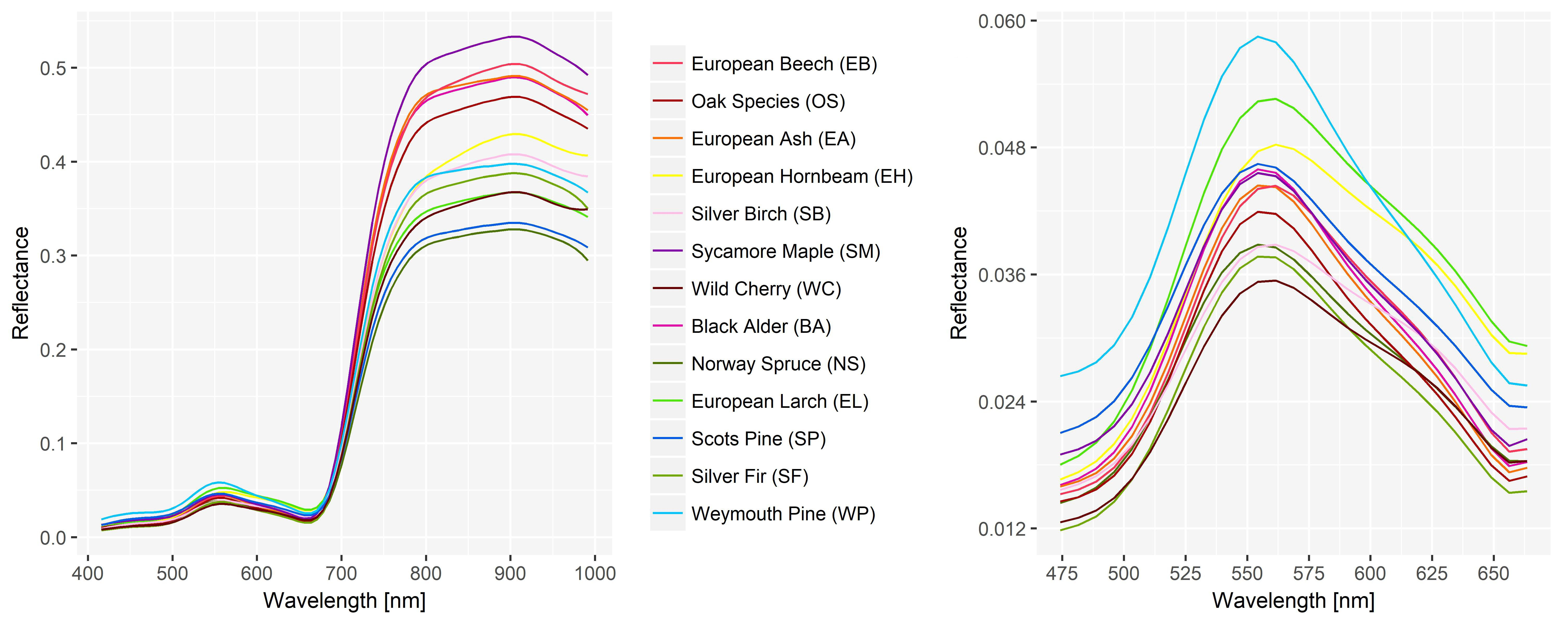
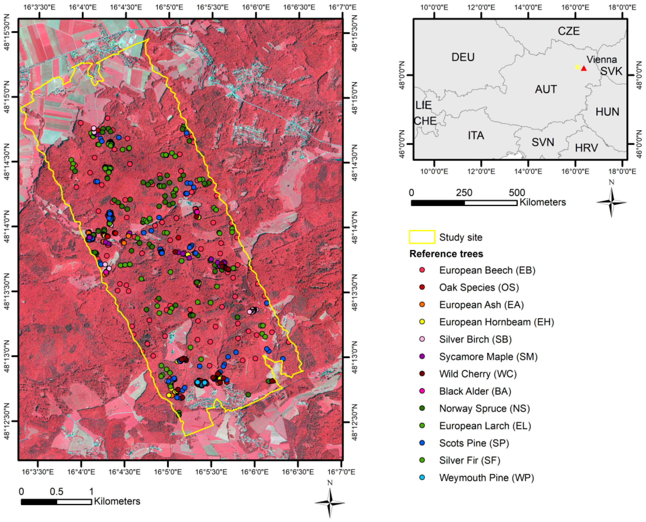
The study site is located in the Austrian province of Lower Austria and covers an area of 1050 ha (Figure 1). The area is a composite of forested, agricultural and urban areas with buildings and roads. The elevation of the hilly terrain ranges between 250 and 600 m above sea level. The area can be allocated to the colline and submontane altitudinal belt. The annual rainfall ranges from 700 to 1,000 mm and precipitation peaks in July. The dominating soils are luvisol and pseudogley. Naturally, the forest is dominated by sessile oak-hornbeam forests, alder-ash forests as well as beech forests with an admixture of sessile oak, ash and maple [32]. In the areas with ongoing timber production, pure spruce, pine and larch stands can be found.

The study site is located in the ‘Wienerwald’, which became a UNESCO Biosphere Reserve in 2005. The reserve is divided into multiple patches. Each one is allocated to one of three different zones, depending on the priorities for the implementation of the biosphere reserve objectives. A large part in the South of the study site is contained by a core region. Core regions are the supposed ‘primeval forests of tomorrow’, which is why silvicultural management has stopped since 2005 [33,34]. A small stretch in the North-West is located in one of the buffer zones, which are not inherently connected to management limitations. The forested part of the transition area of the study site is managed by the Austrian state forest enterprise. The geographical location of the study site is presented in Figure 1.

2.2. Remote Sensing Data

Airborne data were recorded by Airborne Technologies. Hyperspectral data were acquired on 25 August 2016 under cloudless conditions with a Hyspex VNIR 1600 push broom sensor that was mounted on a Tecnam MMA aircraft. The sensor covers the electromagnetic spectrum from 415 nm to 991 nm and provides data with 160 spectral bands, each with a spectral width of 3.7 nm. During the overflight, 18 flight strips were generated with solar azimuth angles between 145° and 165° and solar zenith angles between 47.8° and 51.1°. The average flying altitude was 830 m.a.s.l. and the average flying speed was 56 m/s. However, the high flight speed and altitude interfered with the high spectral resolution of the VNIR sensor. Therefore, two VNIR bands at a time needed to be fused during the pre-processing, resulting in a reduction of the original 160 spectral bands to 80 bands. The pixel size was approximately 0.4 m.

Airborne laser scanning data were acquired during the same flight using a RIEGL LMS-Q680i sensor. The point cloud featured an average point density of 15 points/m² and was used to create Digital Surface and Digital Terrain Models (DSM, DTM) of 0.5 m spatial resolution.

The hyperspectral data were pre-processed involving atmospheric correction and mosaicking. First, individual images were corrected for atmospheric effects using ATCOR4 [35,36]. After this, flight strips were aligned to create a seamless combined image (mosaicking) using the ENVI software (Exelis Visual Information Solutions, Boulder, CO, USA).

2.3. Forest Mask

To isolate the forested areas within the hyperspectral data for subsequent segmentation, a forest mask was created. The basic components of the final forest mask were two sub-masks: (1) a canopy height model (CHM)-based mask, and (2) a Normalized Difference Vegetation Index (NDVI)-based mask. To derive the CHM layer, the difference between DSM and DTM was calculated. The CHM-based mask only included and assembled pixels with a height of at least 3 m. With respect to the second sub-mask, pixels with NDVI values ≥0.6 were considered as being forested. For the final forest mask, the intersection of the CHM- and vegetation-based masks was used. According to this forest mask, 8.4 km² of the 10.5 km² study site are covered by trees. Subsequently, small grasslands, road strips and shadows were eliminated. Elimination was based on the results of a pixel-based Random Forest classification which distinguished the following classes: reference tree classes, shadows, streets, and grasslands. We checked visually that the forested area was well covered.

2.4. Reference Data

A reference shapefile with 287 forest stand polygons and information on the relative shares of 38 tree species was provided by the Austrian state forest enterprise. The shapefile refers to the situation in 2008 and covers the study area. However, the study was mainly focused on middle-age and mature stands and therefore only little changes of the species composition over time can be expected. Of the 38 recorded species, 23 were attributed to at least one of the mentioned 287 polygons. Only very few species grew in pure stands.

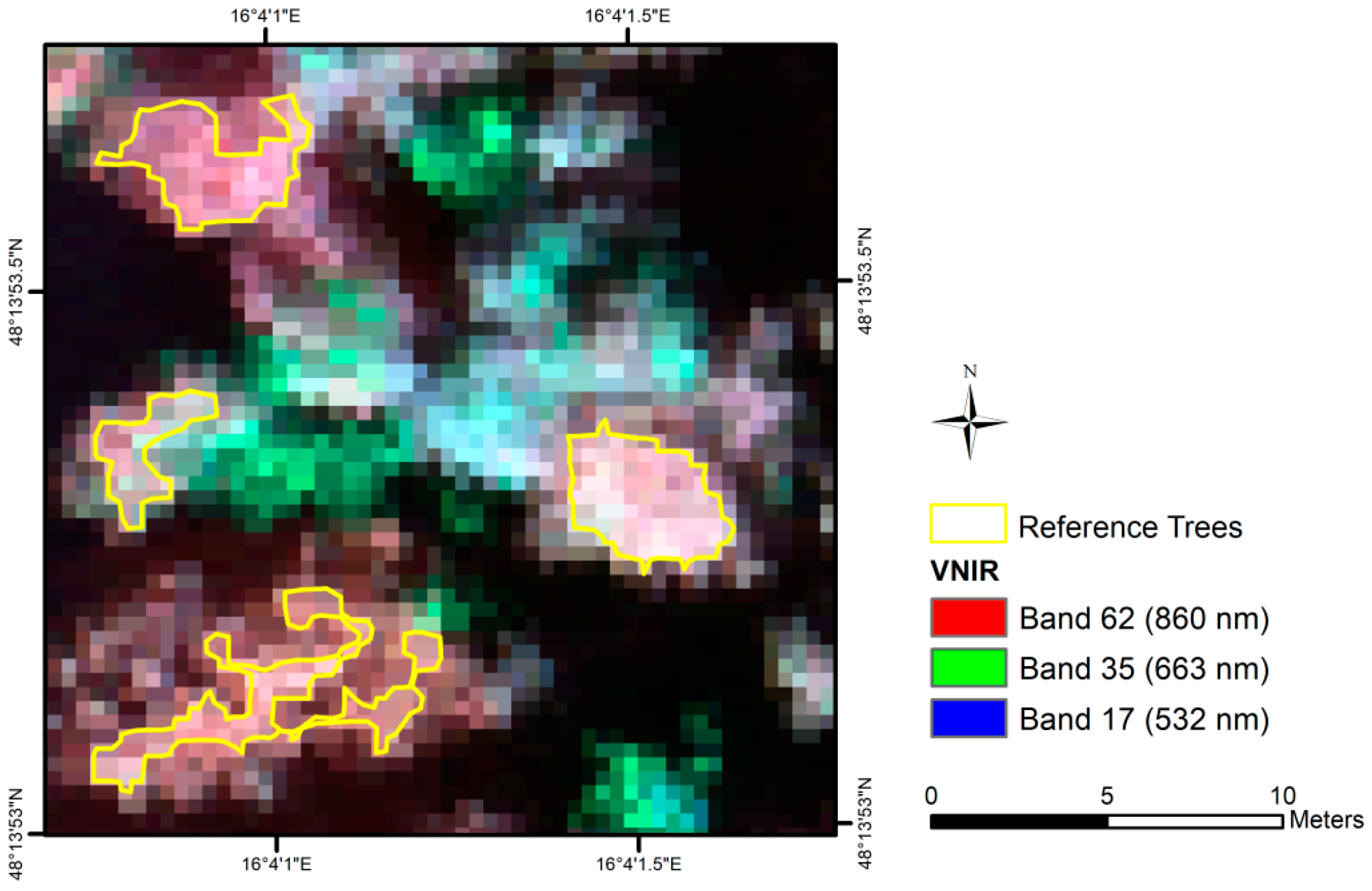
By using reference polygons that were provided by the forest enterprise, detailed reference data were collected during field work in summer 2017. To achieve a decent representation of all tree species in the classification, we decided to exclude all species with less than 20 reference samples. Subsequently, the reference trees were delineated manually in ArcGIS (ESRI 2011). Examples are shown in Figure 2. Upon delineation, only sunlit portions of each crown were considered, which served to decrease intra-crown and intra-species variation. The number and species of the reference trees are given in

Table 1. Overview of the general characteristics of the reference tree species and the respective class sizes.

Common Name	Acronym	Scientific Name	Type	Number
European beech	EB	Fagus sylvatica	Broadleaf	99
Oak species *	OS	Quercus sp.	Broadleaf	64
European ash	EA	Fraxinus excelsior	Broadleaf	44
European hornbeam	EH	Carpinus betulus	Broadleaf	43
Silver birch	SB	Betula pendula	Broadleaf	41
Sycamore maple	SM	Acer pseudoplatanus	Broadleaf	40
Wild cherry	WC	Prunus avium	Broadleaf	37
Black alder	BA	Alnus glutinosa	Broadleaf	33
Norway spruce	NS	Picea abies	Conifer	83
European larch	EL	Larix decidua	Conifer	83
Scots pine	SP	Pinus sylvestris	Conifer	78
Silver fir	SF	Abies alba	Conifer	30
Weymouth pine	WP	Pinus strobus	Conifer	24

* Sessile oak (Q. petraea), Pedunculate oak (Q. robur), Austrian oak (Q. cerris).

. In total, 699 reference polygons were finally available for the study, and each were assigned to one of 13 tree species (eight broadleaf, five coniferous).

2.5. Workflow Description

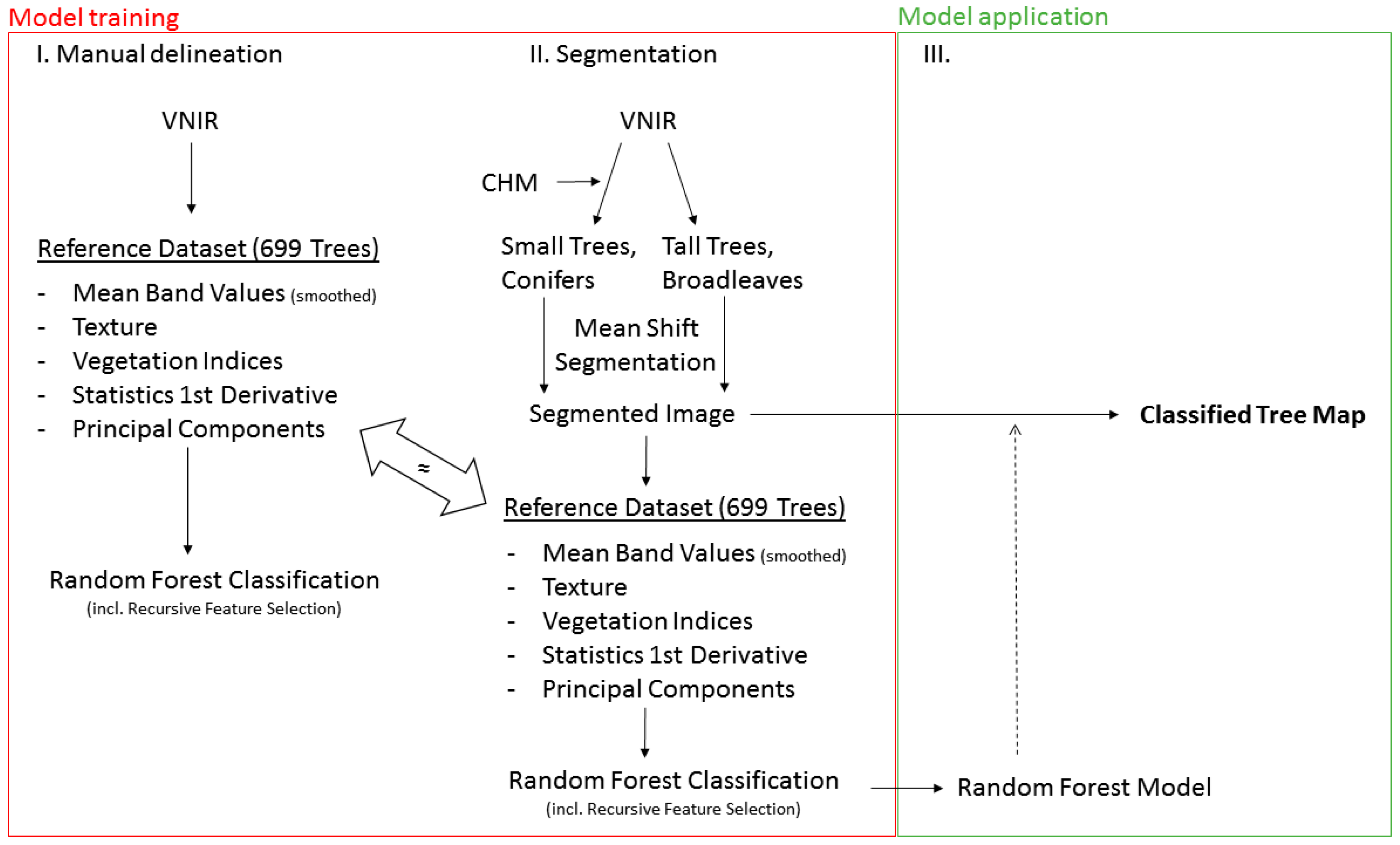
In this work, a three-step approach was followed (Figure 3). First, a Random Forest classifier was trained with the 699 manually delineated reference trees using 202 predictor variables. This step served to evaluate the classification performance for optimally delineated tree crowns. After this, the entire study area, and all of the trees within the study area, were automatically segmented into image objects. The segments corresponding to the manually delineated crowns (highest amount of overlapping area) were selected and were used to create an additional Random Forest model. By comparing the classification results it was checked how strongly the classification accuracy was impaired by the automatic segmentation of the reference trees. To generate a wall-to-wall tree species map, the Random Forest model that was trained on the segmented reference trees was applied to all of the automatic generated segments.

2.6. Noise Removal

Smoothing was applied as even atmospherically corrected reflectance data contain noise. Without smoothing, the noise would be passed on to all classification features. Smoothing is based on the assumption that in the absence of noise—the process underlying the data would result in a smooth curve [28]. The Whittaker smoother is well suited for this task [37]. The smoother balances fidelity to the data with the smoothness of the resulting curve and has the ability to automatically interpolate between missing values [38,39]. The algorithm was executed on the mean reflectance values of each tree crown using the R function miwhitatzb1 [40]. The smoothing was done in one iteration and the parameter (λ) was set to 12.

2.7. Feature Extraction

A large number of features was extracted from the hyperspectral data cube (

Table 2. Number of variables calculated per object and type of variable.

	Reflectance Values	1st Derivatives	Vegetation Indices	Textural Metrics	Principal Components
Number of Variables	80	4	22	16	80

). Besides the smoothed reflectance values, these were statistics of the first derivative of the mean spectral signature (minimum, maximum, mean, standard deviation), vegetation indices (

Table A1. Names, equations and references for the 22 vegetation indices used in this study.

Index	Equation	Reference
Ratio Vegetation Index	$RVI=\frac{{\rho }_{801.99 \mathrm{nm}}}{{\rho }_{678.11 \mathrm{nm}}}$	[81]
Difference Index	$NIR-R={\rho }_{772.84\mathrm{nm}}-{\rho }_{663.54\mathrm{nm}}$	[82]
Normalized Difference Vegetation Index	$NDVI=\frac{{\rho }_{801.99\mathrm{nm}}-{\rho }_{678.11 \mathrm{nm}}}{{\rho }_{801.99\mathrm{nm}}+{\rho }_{678.11 \mathrm{nm}}}$	[83]
Green-Red Difference Index	$GRR=\frac{{\rho }_{561.52 \mathrm{nm}}-{\rho }_{663.54 \mathrm{nm}}}{{\rho }_{561.52 \mathrm{nm}}+{\rho }_{663.54 \mathrm{nm}}}$	[82,84]
Difference Difference Vegetation Index	$DD=(2\ast {\rho }_{947.73 \mathrm{nm}}-{\rho }_{750.98 \mathrm{nm}})-({\rho }_{648.97 \mathrm{nm}}-{\rho }_{546.95 \mathrm{nm}})$	[85]
Atmospherically Resistant Vegetation Index	$ARVI=\frac{{\rho }_{867.57\mathrm{nm}}-(2\ast {\rho }_{663.54\mathrm{nm}}-{\rho }_{466.79\mathrm{nm}})}{{\rho }_{867.57\mathrm{nm}}+(2\ast {\rho }_{663.54\mathrm{nm}}-{\rho }_{466.79\mathrm{nm}})}$	[86]
Green Atmospherically Resistant Vegetation Index	$GARI=\frac{{\rho }_{750.98\mathrm{nm}}-({\rho }_{546.95\mathrm{nm}}-({\rho }_{466.79\mathrm{nm}}-{\rho }_{670.83\mathrm{nm}}))}{{\rho }_{750.98\mathrm{nm}}+({\rho }_{546.95\mathrm{nm}}-({\rho }_{466.79\mathrm{nm}}-{\rho }_{670.83\mathrm{nm}}))}$	[87]
Green Normalized Difference Vegetation Index	$GNDVI=\frac{{\rho }_{750.98\mathrm{nm}}-{\rho }_{546.95 \mathrm{nm}}}{{\rho }_{750.98\mathrm{nm}}+{\rho }_{546.95 \mathrm{nm}}}$	[88]
Visible Atmospherically Resistant Index	$VARI=\frac{{\rho }_{561.52 \mathrm{nm}}-{\rho }_{663.54 \mathrm{nm}}}{{\rho }_{561.52 \mathrm{nm}}+{\rho }_{663.54 \mathrm{nm}}-{\rho }_{488.66 \mathrm{nm}}}$	[89]
Enhanced Vegetation Index	$EVI=2.5\ast \frac{{\rho }_{867.57 \mathrm{nm}}-{\rho }_{648.97 \mathrm{nm}}}{{\rho }_{867.57 \mathrm{nm}}+6\ast {\rho }_{648.97 \mathrm{nm}}-7.5\ast {\rho }_{466.79 \mathrm{nm}}+1}$	[90]
2-band Enhanced Vegetation Index	$EVI2=2.5\ast \frac{{\rho }_{867.57 \mathrm{nm}}-{\rho }_{648.97 \mathrm{nm}}}{{\rho }_{867.57 \mathrm{nm}}+2.4\ast {\rho }_{648.97 \mathrm{nm}}+1}$	[91]
Photochemical Reflectance Index	$PRI=\frac{{\rho }_{532.38\mathrm{nm}}-{\rho }_{568.81 \mathrm{nm}}}{{\rho }_{532.38\mathrm{nm}}+{\rho }_{568.81 \mathrm{nm}}}$	[92,93]
Red Edge Normalized Difference Vegetation Index	$RENDVI=\frac{{\rho }_{750.98\mathrm{nm}}-{\rho }_{707.26\mathrm{nm}}}{{\rho }_{750.98\mathrm{nm}}+{\rho }_{707.26\mathrm{nm}}}$	[94]
Modified Simple Ratio	$mS{R}_{705}=\frac{{\rho }_{750.98 \mathrm{nm}}-{\rho }_{444.93 \mathrm{nm}}}{{\rho }_{707.26\mathrm{nm}}-{\rho }_{444.93 \mathrm{nm}}}$	[95]
Modified Normalized Difference Index	$mN{D}_{705}=\frac{{\rho }_{750.98 \mathrm{nm}}-{\rho }_{707.26 \mathrm{nm}}}{{\rho }_{750.98 \mathrm{nm}}+{\rho }_{707.26\mathrm{nm}}-2\ast {\rho }_{444.93 \mathrm{nm}}}$	[95]
Green Ratio	$GR=\frac{{\rho }_{546.95 \mathrm{nm}}}{{\rho }_{663.54 \mathrm{nm}}}$	[15]
Blue Ratio	$BR=\frac{{\rho }_{663.54\mathrm{nm}}}{{\rho }_{481.37 \mathrm{nm}}}\ast \frac{{\rho }_{546.95\mathrm{nm}}}{{\rho }_{481.37\mathrm{nm}}}\ast \frac{{\rho }_{721.84\mathrm{nm}}}{{\rho }_{481.37\mathrm{nm}}}\ast \frac{{\rho }_{831.14\mathrm{nm}}}{{\rho }_{481.37\mathrm{nm}}}$	[15]
Red Ratio	$RR=\frac{{\rho }_{831.14\mathrm{nm}}}{{\rho }_{663.54\mathrm{nm}}}\ast \frac{{\rho }_{546.95\mathrm{nm}}}{{\rho }_{663.54\mathrm{nm}}}\ast \frac{{\rho }_{831.14\mathrm{nm}}}{{\rho }_{721.84\mathrm{nm}}}$	[15]
Infrared Percentage Vegetation Index	$IPVI=\frac{{\rho }_{801.99 \mathrm{nm}}}{{\rho }_{801.99 \mathrm{nm}}+{\rho }_{678.11 \mathrm{nm}}}$	[96]
Normalized Difference Red Edge Index	$NDRE=\frac{{\rho }_{787.42 \mathrm{nm}}-{\rho }_{721.84 \mathrm{nm}}}{{\rho }_{787.42 \mathrm{nm}}+{\rho }_{721.84 \mathrm{nm}}}$	[97]
Plant Senescence Reflectance Index	$PSRI=\frac{{\rho }_{678.11 \mathrm{nm}}-{\rho }_{503.23 \mathrm{nm}}}{{\rho }_{750.98 \mathrm{nm}}}$	[98]
Weighted Difference Vegetation Index	$WDVI={\rho }_{845.71\mathrm{nm}}-\frac{\rho soi{l}_{867.57 \mathrm{nm}}}{\rho soi{l}_{685.4 \mathrm{nm}}}\ast {\rho }_{678.11\mathrm{nm}}$	[99,100,101]

), textural metrics and principle components. All of the features were generated at object-level only and by using previously smoothed spectra. Object-level information was generated using simple value averaging.

Texture describes tone changes within an image (‘granularity’), i.e., how ‘smooth’ or ‘coarse’ an image appears. With a scale large enough to picture objects of interest over the extent of multiple pixels, texture differences between these objects frequently constitute a distinctive feature [41].

To calculate texture metrics, the ‘Haralick Texture [42] Extraction’ (HTE) application as implemented in the Orfeo ToolBox (OTB) was run [43]. Red (700 nm) and near-infrared bands (846 nm) were selected for this application. As it generated the most appealing output layers (visual inspection), the radius for texture extraction was set to three pixels. Corresponding to the maximum pixel values of each band, the input image maxima were specified as 15,132 (700 nm) and 15,010 (846 nm). For all other parameters default the values were kept. The ‘simple’ mode of the HTE application was chosen for analysis as its texture features showed the most variability. The ‘simple’ mode yields eight textural feature layers for each spectral band (Energy, Entropy, Correlation, Inverse Difference Moment, Inertia, Cluster Shade, Cluster Prominence and Haralick Correlation).

To create variables with potentially higher (condensed) information content, a Principal Component Analysis (PCA) was performed on the atmospherically corrected and mosaicked VNIR data [44]. During this, different amounts of information from the input (bands) are merged into separate uncorrelated principal components [19]. As the computation of principal components for the whole VNIR data would have needed high amounts of memory space, the transformation matrix was determined for an image subset (0.6 km²), which featured only forest. The PCA was done in R using the function prcomp from the immanent ‘stats’ package. Scaling was enabled which eliminates the unit of measurement and thereby makes reflectance values from different bands with different value ranges comparable [45]. The resulting transformation matrix was used to calculate principal components across the image extend.

2.8. Segmentation

The (large scale) mean shift algorithm was applied to the hyperspectral data twice. First, to define strata of (i) small broadleaf or conifer and (ii) high broadleaf stands and a second time to delineate the individual tree crowns within the strata. The first segmentation was necessary as when the mean shift algorithm was applied to the complete hyperspectral data, we found that segmentation parameters, which were suitable for conifers and trees with a rather small crown, left trees with a wide crown over-segmented. It was thereby decided to apply different segmentation parameters to the mentioned groups (small broadleaf or conifer, high broadleaf). A conifer of any height was assigned to the first group (small broadleaf or conifer), while depending on its height—a broadleaf tree was assigned to either the first or the second group. Tree height was considered proxy for tree age, which in turn was considered a proxy for tree crown size. Once, the strata were established, the mean shift algorithm was applied a second time to delineate the individual tree crowns within the strata (using strata-specific parameters) and to thereby automate the tree crown delineation process.

For both segmentation purposes, the mean shift algorithm was used. The mean shift algorithm [46,47] is a non-parametric method for locating the maxima of a density function [48]. Upon mean shift image segmentation, the mean of all the pixel values within a defined circular window around the starting point is calculated. The extent of the window is defined by a spatial and spectral distance. The center of the window is next shifted to the point corresponding to the previously determined mean. This process is repeated until the maximum number of iterations is reached or the window does not significantly move anymore. At this point, an adjustable convergence threshold defines what should be considered as a significant move. Upon clustering, those pixels whose windows got shifted to the same location are grouped together.

For applications over large areas, it has to be considered that the basic mean shift algorithm is unstable due to its tile-wise computation of images. Besides other modifications, the large scale mean shift (LSMS) algorithm [48] generates overlapping tiles, assuring that the surroundings of the border segments from one tile are also explored in another. This prevents a false generation of segment borders at tile borders. Hence, for the generation of the strata, the four-stage LSMS as implemented in the Orfeo toolbox was used. In recent years, LSMS was used for several forest-related analyses of earth observation data [49,50,51]. However, to our knowledge there are still no studies using the mean shift algorithm for the delineation of individual tree crowns.

2.8.1. Stratification

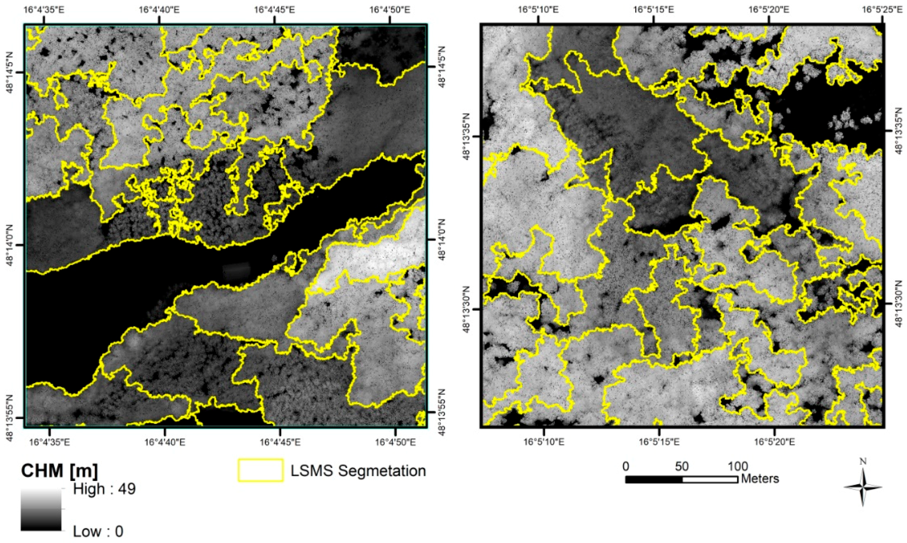
Before delineating individual crowns, we first used the CHM to differentiate stands with mainly high and mainly small trees. This permits combining small broadleaf stands and conifer stands into one stratum for optimum segmentation and classification results at tree level (same for the high broadleaf stands). Acceptable segmentations (visual inspection) were obtained using a spatial radius of 12, a range radius of 3, a minimum object size of 20,000 and maximum 50 iterations (

Table 3. Parameters of the mean shift segmentations for the conifer or small broadleaf and high broadleaf stands (upper part), and the delineation of the individual tree crowns (lower part).

Purpose	Parameter	Height Separation
	Spatial Radius	12
Strata definition	Range Radius	3
	Minimum Object Size	20,000
		Conifer or small broadleaf	High broadleaf
	Spatial Radius	2	2
Tree crown delineation	Range Radius	1	2
	Minimum Object Size	5	10

). Figure 4 gives an idea of the sensitivity of the segmentation. Segments of the high and small trees were separated by applying a threshold of 10 m on the mean height of each segment.

Conifers were separated from broadleaved trees using a pixel-based Random Forest classification. The model was trained using reference data of the following classes: broadleaf trees, coniferous trees, shadow, non-forest vegetation and infrastructure/houses. The pixel-based classification of the VNIR data cube had an overall accuracy of 98.4% (CI = 98.3%, 98.4%;) and a Cohen’s kappa of 0.974. The producer and user accuracies of the conifer class were 87.2% and 94.0%, respectively.

Finally, the shapes indicating small broadleaf or conifer stands were merged. The merger served to indicate the areas in the VNIR data that were designated for the segmentation with a more conservative set of parameters, while the inverse of these areas was used for the segmentation of the high broadleaf stands.

2.8.2. Segmentation of Individual Tree Crowns

Within the two strata, the mean shift algorithm was used to delineate the individual tree crowns. The strata-specific parameters are listed in Table 3 (lower part). The parameters take into account that young (small) broadleaf trees and conifers are best delineated using a small parameter for minimum object sizes (and range radius), compared to larger crowns that are typical for higher trees and broadleaf species.

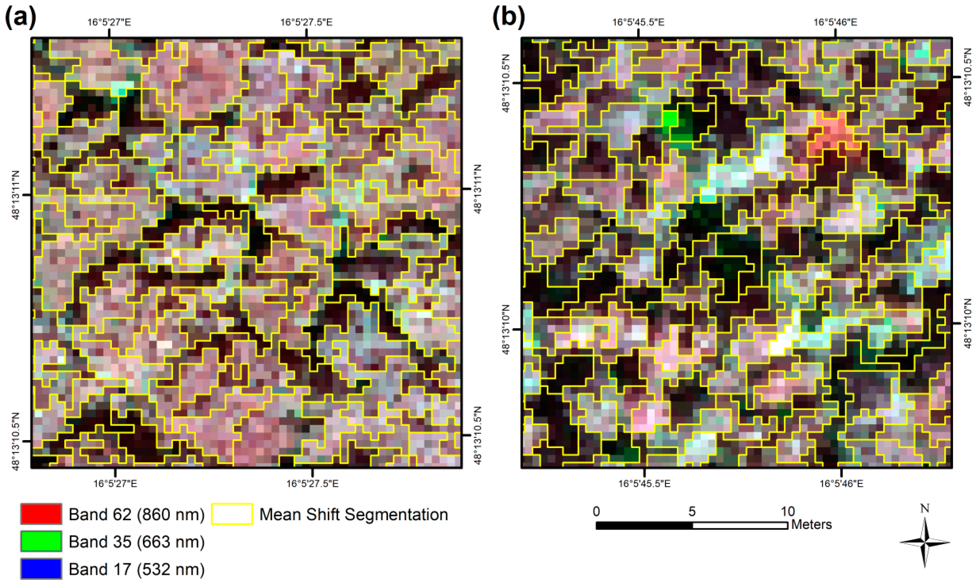
Mean shift segmentation generated 1,596,727 segments with a mean area of 3.65 m². The average object size in the small broadleaf or conifer strata was 2.65 m², compared to 4.06 m² for the high broadleaf strata. Figure 5 gives an idea about the performance of the selected parameters.

2.9. Random Forest Classification

The Random Forest algorithm [29] has gained popularity in remote sensing and is frequently used for the classification of tree species [1,4]. The algorithm constructs hundreds of decision trees based on bootstrap samples that were randomly created from the original dataset. Observations within each bootstrap sample account for about two-thirds of all observations within the original dataset and are drawn with replacement. Random Forest uses each decision tree for the classification of the observations that were not part of the corresponding bootstrap sample (Out-of-bag (OOB) data) [29].

Random Forest deviates from classical bagging algorithms insofar as—to prevent a correlation between the decision trees—it does not consider all input variables (features) for the construction of each decision tree, but only a random selection of these. For a dataset with p input variables and a categorical response variable, the number of features that are considered within each sample is $\sqrt{p}$ by default, with features being selected randomly selected for each bootstrap sample anew [52]. Only one of all the $\sqrt{p}$ variables considered at each node [53,54].

Within the training state of the Random Forest model reference data is used, i.e., all observations feature a true class label. In each decision tree only the corresponding OOB data set is classified. The proportion of matches between majority vote from the OOB results and the true class label is used for accuracy assessment. Due to this built-in validation measure, it becomes unnecessary to set aside a test set [53,55,56].

There are different ways of how the Random Forest algorithm estimates the importance of each input variable for the classification result. One measures the impact that the input variable has on the classification result and is originally called the Margin measure [53], however it is referred to as Mean Decrease in Accuracy (MDA) in e.g., the randomForest R package [57]. The margin of an observation is defined as the number of votes for the true class of the observation minus the number of votes for other classes. In the first step, OOB data is passed down the corresponding decision trees. In the second step, the values of one specific input variable are randomly permuted within the OOB data. Each of the modified OOB datasets is then run down its corresponding unaltered decision tree. The average lowering of the margin across all of the observations upon the permutation of variable values is a measurement of the relative importance of the input variable for classification. A large decrease of the average margin corresponds to a high importance [53]. As it is customary for classification studies, the results of a classification are displayed in a confusion matrix, featuring the producer’s, the user’s and the overall accuracy as well as Cohen’s kappa coefficient.

For this study, the algorithm was executed in R version 3.3.3 [58]. We used the randomForest() function from the identically named package by Liaw and Wiener [57]. The function confusionMatrix from the ‘caret’ package [59] was used for the extraction of Cohen’s kappa and the ‘raster’ package [60] was used for data preparation. The default settings of the two tuning parameters for randomForest were kept: the number of decision trees to grow (ntree = 500) and the number of variables used to split at each node (mtry = $\sqrt{p}$). The setting does not only ensure comparability with other studies, but also proofed to lead to reasonable results in studies that experimented on these values [4,61].

To find the optimum feature combination, a recursive feature selection was applied [62]. The backward features selection starts with a model that is based on all of the input features and makes a step-wise reduction by removing each time the least important variable based on the MDA values which are recalculated at each step [63,64,65]. At the end, the model with the lowest number of input features which reaches min 97.5% of the maximum OOB overall accuracy is used.

To obtain a quality indicator in the model application step, classification reliability was calculated as the share of votes for the class with the highest number of votes minus the share for the class with the second highest number of votes [50,65]. This yields a reliability value ranging between 1 and 0, with 1 indicating a high and 0 indicating a low classification reliability.

3. Results

3.1. Spectral Signatures of Tree Species

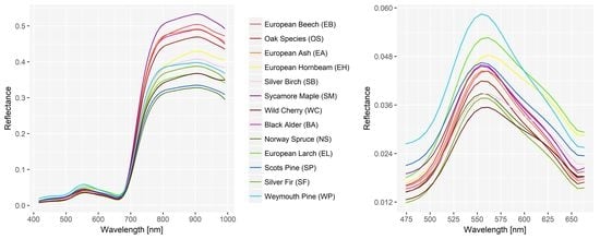
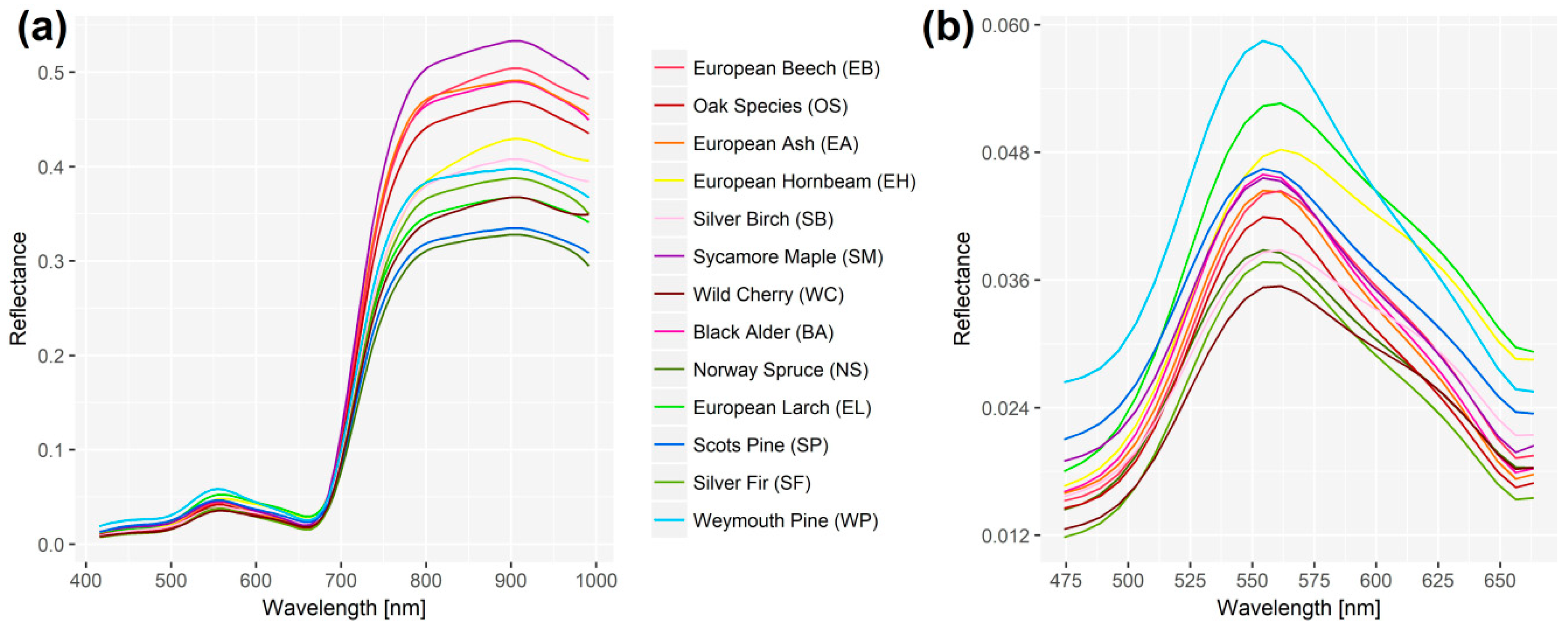
The complete spectral signatures for each of the 13 investigated tree species are featured in Figure 6a. The reflectance values of the different species are particularly widespread around wavelengths > 800 nm. The reflectance of sycamore maple is comparatively high, while the opposite is true for Norway spruce. For the spectral interval between 800 and 1000 nm, the reflectance values of broadleaves are generally higher than the corresponding values of conifers. However, there is some overlap, e.g. around the comparatively low reflectance values of wild cherry in the spectral interval between 800 and 991 nm. For the visible range, the spectral signatures around the green peak at 560 nm are shown in Figure 6b. Directly at the peak, the ranking of the maximum reflectance values is very different. Three of the four highest reflectance values were obtained for coniferous species, while the lowest ones were featured by wild cherry.

3.2. Classification of Manually Delineated Reference Trees

The results of the classification of manually delineated reference trees are given in

Table 4. Confusion matrix for the VNIR (all) classification based on the manually delineated tree crowns. The gray lines separate coniferous and broadleaf trees. Tree species are abbreviated as follows: EB = European beech, OS = oak species, EA = European ash, EH = European hornbeam, SM = sycamore maple, SB = silver birch, WC = wild cherry, BA = black alder, NS = Norway spruce, EL = European larch, SP = Scots pine, SF = silver fir, WP = Weymouth pine. Other abbreviations in the table: PA = producer’s accuracy, OA = overall accuracy, UA = user’s accuracy, κ = Cohen’s kappa.

		Reference
		EB	OS	EA	EH	SB	SM	WC	BA	NS	EL	SP	SF	WP	∑	UA [%]
Classification	EB	88	5	3	4	0	1	1	1	0	0	0	1	0	104	84.6
	OS	4	55	1	0	0	1	0	1	0	0	0	0	0	62	88.7
	EA	2	1	32	0	0	0	0	1	0	0	0	0	0	36	88.9
	EH	1	1	0	39	0	0	1	0	0	0	0	0	0	42	92.9
	SB	1	0	0	0	41	0	1	1	0	0	0	0	0	44	93.2
	SM	2	2	4	0	0	37	0	2	0	0	0	0	0	47	78.7
	WC	0	0	0	0	0	0	33	0	0	0	0	0	0	33	100.0
	BA	1	0	4	0	0	1	0	27	0	0	0	0	0	33	81.8
	NS	0	0	0	0	0	0	0	0	78	2	1	0	0	81	96.3
	EL	0	0	0	0	0	0	1	0	3	81	0	0	0	85	95.3
	SP	0	0	0	0	0	0	0	0	2	0	77	0	0	79	97.5
	SF	0	0	0	0	0	0	0	0	0	0	0	29	0	29	100.0
	WP	0	0	0	0	0	0	0	0	0	0	0	0	24	24	100.0
∑		99	64	44	43	41	40	37	33	83	83	78	30	24	699
PA [%]		88.9	85.9	72.7	90.7	100.0	92.5	89.2	81.8	94.0	97.6	98.7	96.7	100.0
OA [%]		91.7
κ		0.909

. Hereafter, this classification will be referred to as the ‘VNIR (all)’, compared to the results that were obtained from the automatically segmented tree crowns (labeled as ‘VNIR (all—mean shift)’). The lowest user’s accuracy was obtained for sycamore maple (78.7%) and is mainly owed to misclassifications of European ash. The maximum value (100.0%) was achieved for Weymouth pine, silver fir and wild cherry. The classification of Weymouth pine and silver birch yielded a producer’s accuracy of 100.0%. The lowest producer’s accuracy was associated with European ash (72.7%), which was mainly due to the mentioned misclassifications as sycamore maple and black alder. With one misclassification as European beech, silver fir is the only coniferous species that got classified as a broadleaf. There was also only one misclassification of a broadleaf species as a conifer, namely wild cherry as European larch.

Of all 699 reference trees, 58 were misclassified (8.3%). Of these, nine trees were conifers, which corresponds to 3.0% of all conifers in this classification, while a total of 49 broadleaves were misclassified (12.2% of all broadleaves). The overall accuracy of the classification is 91.7% (confidence interval (CI) = 89.4%, 93.6%), while Cohen’s kappa reaches 0.909.

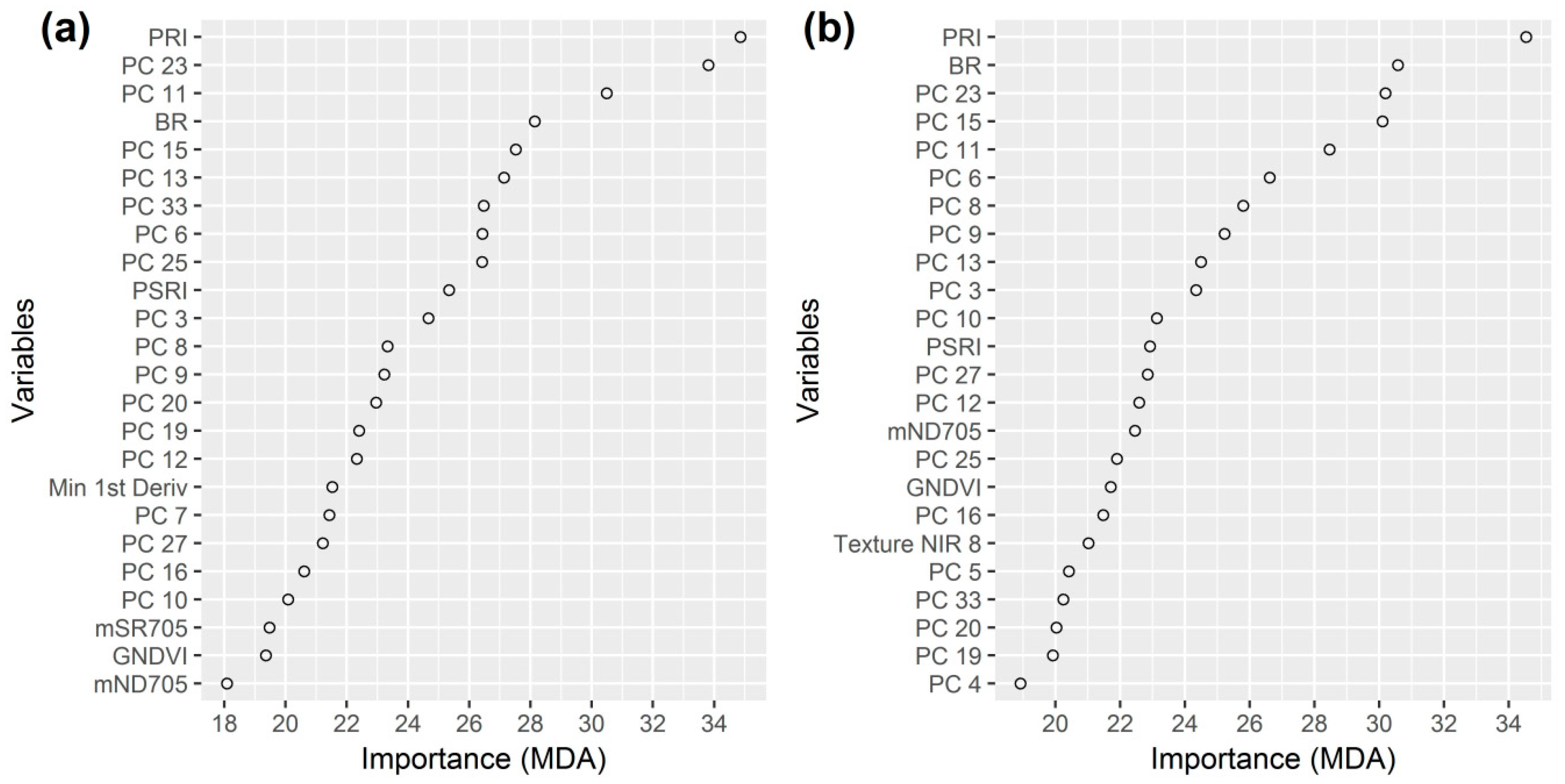
The importance of the 24 variables that are part of the best model are illustrated in Figure 7a. Most of the variables are principal components (17) representing a weighted average of the individual spectral bands. The other variables are vegetation indices (PRI, BR, PSRI, mSR705, GNDVI, mND705) and the minimum of the first derivative. The three most important variables are PRI, PC 23 and PC 11.

To evaluate the potential benefit of adding variables of the four variable groups (i) texture, (ii) statistics of the first derivative, (iii) indices and (iv) principal components—in contrast to using only band values for the classification—the subsets of the reference dataset were also classified. The classification that only used the 80 smoothed bands as an input (‘VNIR (bands)’) yielded an overall accuracy of 58.1% (CI = 54.3%, 61.8%) with a Cohen’s kappa of 0.536. At this, 55.1% of all broadleaves and 24.2% of the conifers were misclassified. Adding texture variables (‘VNIR (bands, texture)’) or statistics of the first derivative to the band values (‘VNIR (bands, 1st derivative)’) did hardly improved the classification results (overall accuracy = 59.4%/59.1% (CI = 55.6%, 63.0%/55.3, 62.8), Cohen’s kappa = 0.550/0.547). Including all 22 vegetation indices (‘VNIR (bands, indices)’), however, improved the result significantly (overall accuracy = 75.5% (CI = 72.2%, 78.7%), Cohen’s kappa = 0.730). With an overall accuracy of 89.3% (CI: 86.7%, 91.5%) and a Cohen’s kappa of 0.882, the best results for these two-variable groups setups were obtained for ‘VNIR (bands, PCs)’. The very best results were obtained by using variables from all of the groups (VNIR (all)). Combining bands, indices and principal components (‘VNIR (bands, indices, PCs)’) resulted in an overall accuracy of 91.0% (CI = 88.6%, 93.0%) and a Cohen’s kappa of 0.901.

3.3. Classification of Mean Shift-Segmented Reference Trees

Using reference trees that were segmented with the mean shift algorithm (‘VNIR (all)—mean shift’), the lowest user’s accuracies were obtained for oak (79.4%). As in the case of the VNIR (all) classification, Weymouth pine was associated with the maximum producer’s and user’s accuracy (100.0%). The lowest producer’s accuracy was obtained for European ash (75.0%), mainly due to misclassifications as black alder, European beech and oak. Silver fir is the only coniferous species that got misclassified as a broadleaf species, namely European beech. Half of the broadleaf species got misclassified as conifers at least once. With this, sycamore maple got most frequently misclassified as a conifer (silver fir). Most misclassified broadleaf species were classified as European larch. Of all 699 reference trees, 74 were misclassified (10.6%). Of these 74 trees, 14 were conifers, which corresponds to 4.7% of all conifers in this classification, while a total of 60 broadleaves were misclassified (15.0% of all broadleaves). The overall accuracy of the classification is 89.4% (CI = 86.9%, 91.6%). Cohen’s kappa reaches 0.883. The confusion matrix is provided in

Table 5. Confusion matrix of the VNIR (all—mean shift) classification based on the automatically segmented tree crowns. The gray lines separate coniferous and broadleaf trees. Tree species are abbreviated as follows: EB = European beech, OS = oak species, EA = European ash, EH = European hornbeam, SM = sycamore maple, SB = silver birch, WC = wild cherry, BA = black alder, NS = Norway spruce, EL = European larch, SP = Scots pine, SF = silver fir, WP = Weymouth pine. Other abbreviations in the table: PA = producer’s accuracy, OA = overall accuracy, UA = user’s accuracy, κ = Cohen’s kappa.

		Reference
		EB	OS	EA	EH	SB	SM	WC	BA	NS	EL	SP	SF	WP	∑	UA [%]
Classification	EB	84	5	3	3	0	1	1	1	0	0	0	2	0	100	84.0
	OS	6	54	3	1	0	2	0	2	0	0	0	0	0	68	79.4
	EA	2	1	33	0	0	1	0	1	0	0	0	0	0	38	86.8
	EH	1	1	0	38	0	0	1	0	0	0	0	0	0	41	92.7
	SB	1	0	0	0	40	0	1	0	0	0	0	0	0	42	95.2
	SM	3	2	2	0	0	31	0	1	0	0	0	0	0	39	79.5
	WC	1	0	0	0	0	1	33	0	0	0	0	0	0	35	94.3
	BA	1	1	3	0	0	2	0	28	0	0	0	0	0	35	80.0
	NS	0	0	0	0	0	0	0	0	77	2	2	1	0	82	93.9
	EL	0	0	0	1	1	0	1	0	4	81	0	1	0	89	91.0
	SP	0	0	0	0	0	0	0	0	2	0	76	0	0	78	97.4
	SF	0	0	0	0	0	2	0	0	0	0	0	26	0	28	92.9
	WP	0	0	0	0	0	0	0	0	0	0	0	0	24	24	100.0
∑		99	64	44	43	41	40	37	33	83	83	78	30	24	699
PA [%]		84.8	84.4	75.0	88.4	97.6	77.5	89.2	84.8	92.8	97.6	97.4	86.7	100.0
OA [%]		89.4
κ		0.883

.

Of all 24 variables selected for the best VNIR (all—mean shift) model, 21 were also among the 24 variables of the best model of the VNIR classification. The three new variables were Texture NIR 8 (Textural feature: Haralick Correlation), PC 5 and PC 4. Similar to previous results, most of the variables are principal components (18). Again, the vegetation index PRI is the most important variable, followed by BR. In total, five vegetation indices are included in the model. The complete variable importance plot is provided in Figure 7b.

3.4. Comparison of Classifications Results for Manually and Automatically Segmented Reference Trees

Table 6. Overall accuracy (OA) and Cohen’s kappa (κ) for classifications of reference trees. The dotted line separates the classifications of the manually delineated reference trees (above) from the classifications of the segmented reference trees (below). Abbreviations are as follows: CI = Confidence Interval, Ind. = Indices, PCs = Principal components, Text. = Texture, 1st Deriv. = 1st Derivative. The best classification is printed in bold.

Classification Designation	Variables	OA [%] (CI [%])	Κ
VNIR (bands)	Bands	58.1 (54.3, 61.8)	0.536
VNIR (bands, 1st derivative)	Bands, 1st Deriv.	59.1 (55.3, 62.8)	0.547
VNIR (bands, texture)	Bands, Text.	59.4 (55.6, 63.0)	0.550
VNIR (bands, indices)	Bands, Ind.	75.5 (72.2, 78.7)	0.730
VNIR (bands, PCs)	Bands, PCs	89.3 (86.7, 91.5)	0.882
VNIR (bands, indices, PCs)	Bands, Ind., PCs	91.0 (88.6, 93.0)	0.901
VNIR (all)	Bands, 1st Deriv., Text., Ind., PCs,	91.7 (89.4, 93.6)	0.909
VNIR (all—mean shift)	Bands, 1st Deriv., Text., Ind., PCs,	89.4 (86.9, 91.6)	0.883

summarizes the classification results that were obtained from all of the classifications of the manually delineated and automatically segmented reference trees. In general, the results of the VNIR (all—mean shift) classification were only slightly worse than the ones obtained for the equivalent manual delineation scenario. For the classifications that were based on manually delineated trees, the results were best upon including all variables, closely followed by the classification using bands, indices and principal components. Using only reflectance values (VNIR (bands)) yielded the worst of all results. A huge difference was found between the results of the four classifications using spectral reflectance values plus one of the four other variable groups (1st derivative, texture, indices, principal components): While the scenarios with indices and principal components generate good results, it does hardly make a difference to the accuracy when texture or statistics of the first derivative are added to the classification.

The classification accuracies of the individual tree species varied between the different classifications. However, some species were repeatedly associated with highest or lowest accuracies. The producer’s accuracy of European ash was the lowest in all eight classifications. The species that were associated with minimum user’s accuracies were European ash, oak and sycamore maple. Both Weymouth pine and Scots pine had the maximum user’s accuracies in four cases. Two times, Scots pine, Weymouth pine, silver birch and European larch were associated with the highest producer’s accuracies. There were only three cases where maximum accuracy values were obtained for a broadleaf species (producer’s accuracy of silver birch (twice), user’s accuracy of wild cherry).

3.5. Importance of Wavelengths for Principal Components

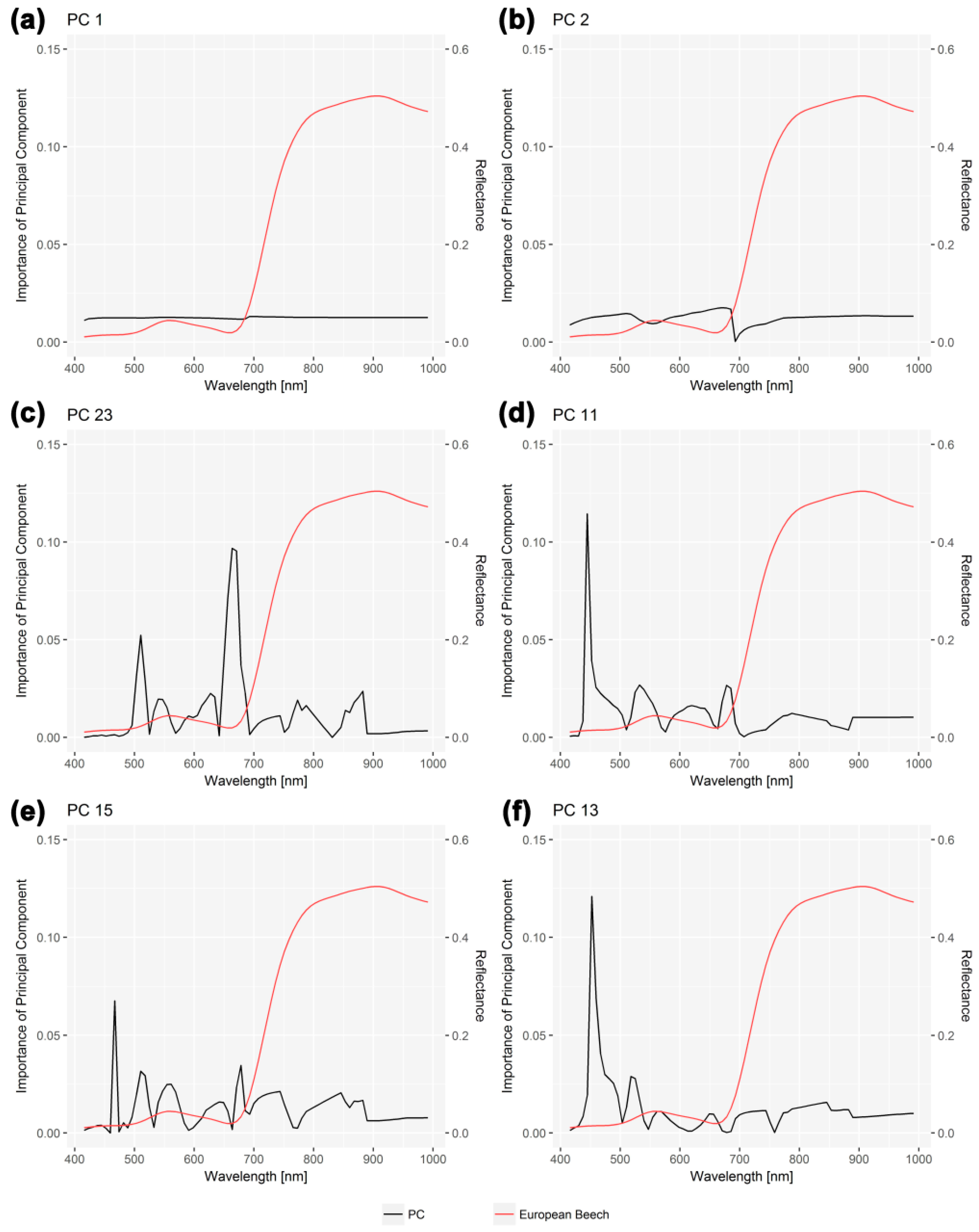
Figure 8 presents the wavelength loadings for the first two principal components (PC 1 and PC 2), as well as the four principle components that were associated with the highest importance in the best model of the VNIR (all) classification (PC 23, PC 11, PC 15 and PC 13). The average spectral signature of European beech was added to the graphs to ease interpretation. The loadings of the first two PCs, particularly PC 1, are very uniform (Figure 8a,b). This implies that these two PCs focus on the overall spectral variability in the data cube without necessarily improving the discrimination of the species. On the contrary, the loadings of the four most important principal components (Figure 8c–f) feature several peaks, indicating that different parts of the electromagnetic spectrum contribute to the separability of the classes. Besides peaks around green wavelengths (500–550 nm), we also note maxima located around blue wavelengths, as well as in the red region of the light spectrum. Compared to the visible spectral range, the near-infrared range seems to store less information that is needed for species discrimination (in this particular case).

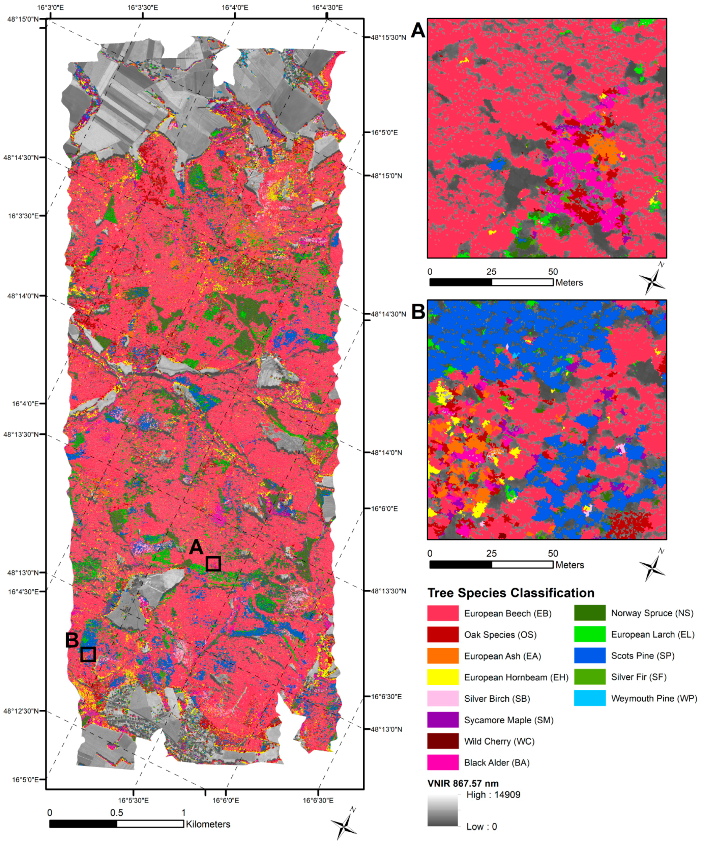
3.6. Wall-to-Wall Mapping on Mean Shift-Segmented VNIR Image

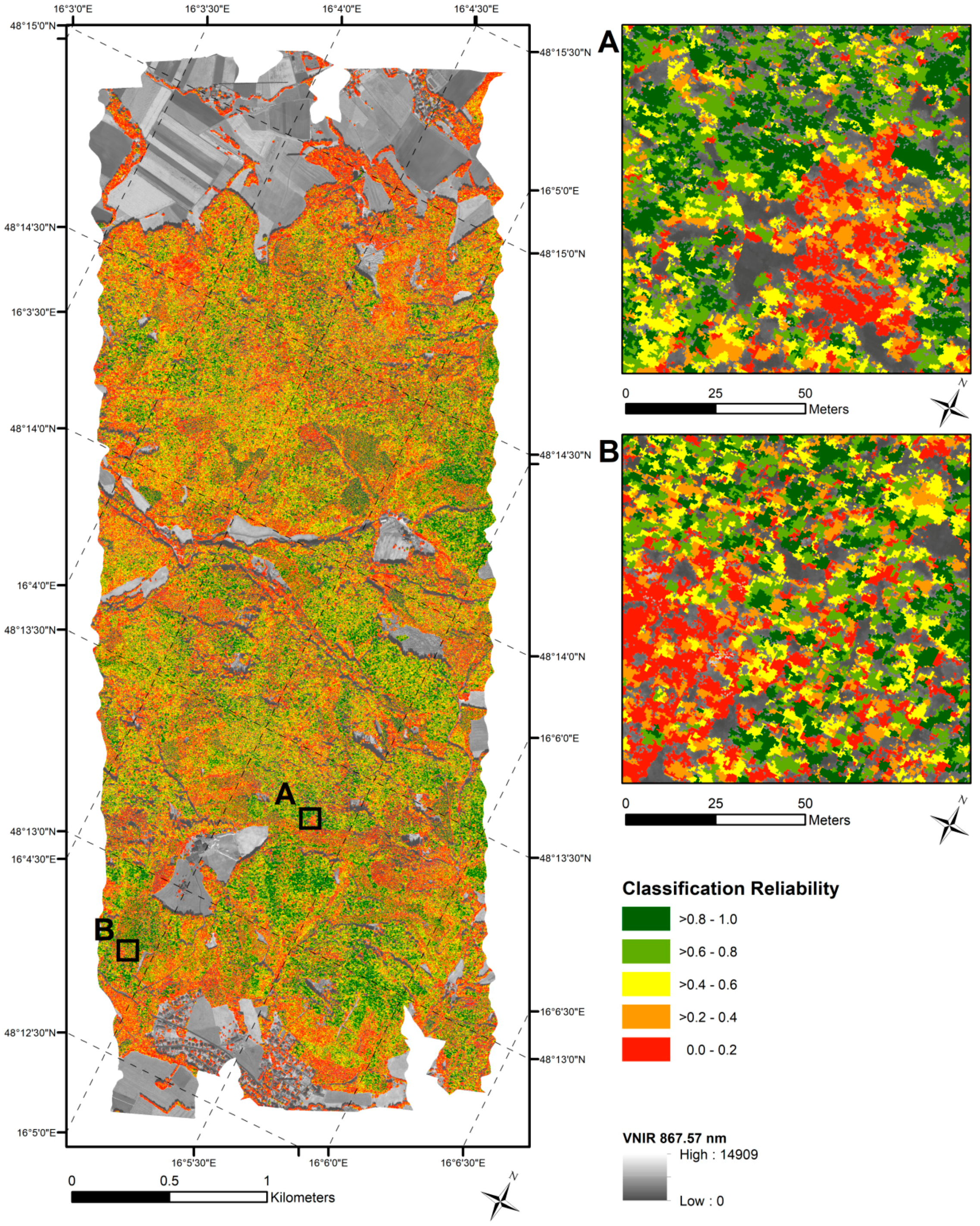
The wall-to-wall tree species and classification reliability maps are presented in Figure 9 and Figure 10. The classification map (Figure 9) shows the high species richness and biodiversity. The corresponding classification reliabilities (Figure 10) demonstrate a large spatial variability. In the upper map detail (A) of Figure 10, an accumulation of segments with low reliabilities can be found (in red). Around this area, high classification reliabilities have been recorded (in green). This pattern can be rediscovered in the upper map detail (A) of Figure 9. High classification reliabilities correspond to an area where all segments were classified as European beech. In contrast, the area of low classification reliability is made up of segments that were mainly classified as black alder, European ash and oak. A similar picture of tree species distribution patterns matching the classification reliabilities is depicted in the second map details (B) where in this case Scots pine being is associated with the highest reliabilities.

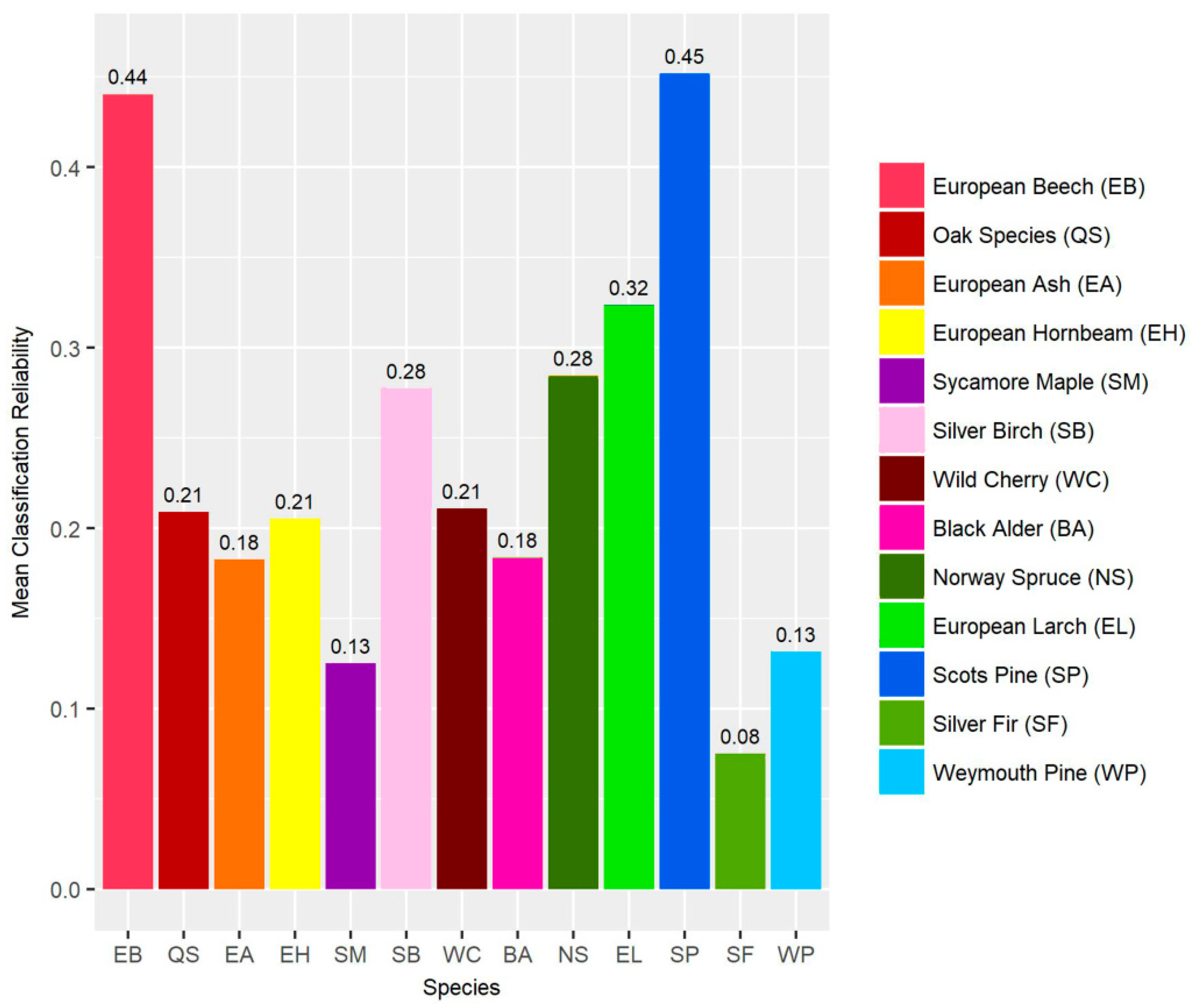
The average classification reliability (=share of votes for the class with the highest number of votes minus the share for the class with the second highest number of votes) of all of the segments is 0.36 with substantial differences for the different species (Figure 11). The highest and lowest mean classification reliability values of the broadleaf species were obtained for European beech (0.44) and sycamore maple (0.13). The corresponding values of conifers were 0.45 (Scots pine) and 0.08 (silver fir).

4. Discussion

The study shows that accurate tree species classification results can be obtained with hyperspectral data, with overall accuracies exceeding 90%. Differences between segmented and manually delineated tree crowns were small and not statistically significant. At the same time, despite the high number of classified tree species (13), our classification results outperformed other studies.

4.1. Classification Accuracies

The high OOB classification accuracies can be first and foremost attributed to the fact that the acquired hyperspectral dataset featured both a high spectral (80 bands, 7.3 nm wide) as well as a high spatial resolution (0.4 m). In other studies, a comparable resolution is usually—if at all—only given for either the spectral or the spatial domain. For example, a pixel-based classification of five tree species with hyperspectral data of 8 m spatial resolution and 125 bands resulted in an overall accuracy of 86% based on an independent validation data set [66]. Fassnacht et al. [67] achieved overall accuracies of 84% to 92% (seven species) and 86% to 97% (five species) with hyperspectral data with 125 bands of 3 to 4 m spatial resolution using different feature selection approaches and an iterative bootstrap classification approach. Richter et al. [27] separated ten broadleaved tree species based on data with 367 spectral bands and 2 m spatial resolution with an overall accuracy of 78.4%. Dalponte et al. [68] obtained a cross validated Cohen’s kappa of 0.890 in a pixel-based classification that was based on hyperspectral data with a spatial resolution of 0.4 m and 160 bands (band width: 3.6 nm), hence using data more similar to ours. However, only three tree species were classified, demonstrating that the excellent spatial and spectral resolution of our dataset cannot be the only reason for our good results. All of these studies used pixel-based approaches to classify hyperspectral data covering VNIR as well as the SWIR region.

On the other hand, also studies based on multispectral data with high spatial resolution (2 m) achieved good classification results. Using WorldView-2 data for the object-based classification of ten tree species, Immitzer et al. [4] obtained an OOB overall accuracy of 82.0%. Other WorldView-2 studies in Central Europe achieved similar results [15,69].

As evident in Table 6, vegetation indices and principal components strongly contributed to the success of our approach. These findings are in line with other studies [66,67]. Beneficial were also the high number of reference samples per class (24 (Weymouth pine) to 99 (European beech)). At the same time, only the sunlit areas of each tree crown were considered when delineating the reference samples. This has also been recommended by other studies [4,23,66] and was done with the ambition to decrease the intra-crown and intra-class variation of the spectral signal due to varying illumination within the canopy. Similarly, the parameters of the segmentation algorithm were set to mimic these manual delineations. Together, these choices have certainly positively contributed to the classification results, although we did not attempt to quantify the contribution of each individual factor.

4.2. Suitability of Hyperspectral Dataset and Segmentation Algorithms

One main objective of the study was to check how much the quality of the classification is affected by replacing manually delineated polygons with segmented reference polygons. Obviously, any observed decrease in accuracy should be traded off against the potential benefits of an automated crown delineation process. For example, only automatic segmentation makes it possible to apply per-tree classification models over large areas, leveraging the full environmental and economic potential of remotely sensed data [70]. With this in mind, the observed loss in classification accuracy was acceptable. Indeed, we only found a slight decrease of the VNIR (all) classification results compared to those that were based on automated segmented reference data (Δ overall accuracy = −2.3 pp, Δκ = −0.026). This decline in classification accuracy can be considered very small, especially in the face of the overlapping confidence intervals (Table 6). Relatively similar classifications using manually and automatically segmented objects were also reported by Dalponte et al. [69]. However, these results were based only on three different tree species.

To generate reasonable tree crown objects with acceptable efforts, while avoiding the pitfalls and challenges of more sophisticated approaches (e.g., [25,71,72]), we chose to implement a stratified approach. We first separated the high and broadleaf stands from the small and/or conifer stands. For this, a LiDAR-based CHM was used, which could, however, easily be replaced by CHMs generated from photogrammetry. The high broadleaf stands were usually made up of relatively large crowns, whereas small trees and conifers generally had small crowns. The tree crown segmentation parameters were fixed accordingly for the two strata. Parameter settings were chosen in a way that the polygons resulting from the segmentation process were as congruent as possible with the manually delineated polygons. For this, over-segmentation was chosen over under-segmentation. Therefore, the majority of the segments are presumably smaller than the corresponding manual objects. In the reference dataset, the average automated generated segment size was around 40% smaller than the manually delineated crowns. As only sunlit areas were included in the manually delineated polygons, it was to be expected that a smaller extent of this polygon (as obtained from our segmentation) would still yield good classification results. No further attempts were made to optimize the tree crown segmentation process, which would be necessary if also the tree number should be counted. One possibility for the optimization of the parameters could be based on the classification results [65]. Another option would be to use unsupervised approaches [73]. Also, with respect to the chosen mean shift segmentation algorithm, we did not study the various existing alternatives [25]. In our understanding, the most appealing advantage of the mean shift algorithm is the fact that minimum object sizes can be deliberately set [74].

4.3. Classification of Tree Species

In all but the VNIR (all) classification, the user’s and producer’s accuracies of the five coniferous species were higher compared to the eight broadleaf species. Similar findings were reported by other studies [23,31,67]. By far the best classification results were obtained for Weymouth pine and Scots pine. The classes with the lowest user’s accuracies, i.e., the classes that the most misclassified trees were assigned to, are European ash, oak and sycamore maple.

The clear superiority of the two coniferous species Weymouth pine and Scots pine is probably related to the distinctiveness of their spectral signatures. By contrast, the intra-class spectral signatures of the mentioned broadleaf species are very diverse and overlap with those of other tree species. Consequently, four of the six trees that were misclassified as black alder in the VNIR (all) classification were European ash, which is a species with a very similar spectral signature.

In the VNIR (all—mean shift) classification, oak was associated with the lowest user’s accuracy, mainly owing to misclassifications of European beech. This was not expected as there seemed to be relatively large spectral differences between the two respective spectral curves (Figure 6). It is possible that the data of some of the reference trees were noisy, which remained unrecognized upon inspection of the average spectral signatures. For example, signal from the soil, smaller trees and other (understory) vegetation might also be featured in the reference dataset due to a loose canopy structure [1,75].

Another possible reason for the high classification accuracy of both Weymouth and Scots pine could be related to the light requirements of these species. Dalponte et al. [6] argue that the low shade tolerance of pines allows them to grow only under good light conditions, which is why these trees are usually less suppressed by neighboring trees. In our study, this could have minimized external perturbations of the spectral signatures of the two pine species. Indeed, the stand where all of the reference Weymouth pines were sampled was comparatively open. Some correlation between light requirement and the accuracies in the VNIR (all) classification could be implied, e.g., by the high producer’s accuracies of the highly light requiring species silver birch (100.0%), Scots pine (98.7%) and European larch (97.6%). Also, the user’s accuracies of sycamore maple (78.7%), European ash (88.9%) and European hornbeam (92.9%) are in line with their rising light requirement (for a ranking of the light requirements of the tree species, see Ellenberg and Leuschner [76]). However, the fact that there are multiple deviations from this supposed relationship suggests that the light requirement of a species is only one factor among others that is relevant for the classification accuracy.

It is a well-known issue that the Random Forest classifier favors the classification of classes with a large number of reference samples—often at the expense of those with less reference samples [77]. In our work, however, both user’s and producer’s accuracies were relatively independent from the sample number. Even the species with relatively few reference samples (≈ n ≤ 30: silver fir, Weymouth pine) appeared to still have had enough samples not to be overwhelmingly affected. Apparently, in our study, the classification success depended more on the distinctiveness of the spectral signatures and much less on the number of reference samples.

Similar to other studies, we evaluated our models only with respect to the chosen classes. The 13 tree species that were included in our study cover the vast majority of the forest. However, we know that more species are present in the forest. For some very rare species that were reported in the dataset from the Austrian state forest enterprise, we were not able to take a sufficient amount of reference samples (≥20). Those species are therefore automatically misclassified, but do not appear in our confusion matrices. The same shortcoming exists for young and/or covered trees. For example, tree age can have effects on the spectral signatures of tree species [12,14]. There were hardly any young trees featured in the reference dataset as their usually small crowns were hard to identify in the data, often overlapping with neighboring tree crowns or even completely hidden. Therefore, it is probable that the accuracy of the model is positively biased.

As expected, the accuracies improved when apart from the spectral reflectance values there were additional variables used for the classifications including a simultaneous feature selection [27,31,68,78]. In particular, the addition of spectral indices and principal components drastically improved the classification results. By contrast, the inclusion of textural metrics and first derivatives only had a small effect. With respect to the textural metrics, it seems that the ratio of object to pixel size was not large enough to produce meaningful additional information [79].

The upswing in accuracies associated with broadleaves was more pronounced than the corresponding values for conifers (VNIR (all)—VNIR (bands): Δ UA_broadleaf = + 42.1 pp, Δ PA_broadleaf = + 45.6 pp, Δ UA_conifer = + 31.1 pp, Δ PA_conifer = + 27.6 pp). These results suggest that conifers can be classified decently already with very basic variables while additional variable are particularly beneficial for the correct classification of broadleaf trees. The correction for background effects through vegetation indices, for example, might be helpful for the classification of relatively open and transparent broadleaf trees, but less beneficial for the classification of the relatively compact conifer canopies.

The achieved classification reliability is additional information which can be important for the interpretation of the classification results or for revising the results [64]. Schultz et al. [65] showed that high reliabilities are positively correlated with a higher amount of correct classification. Species which obtained higher class specific accuracies were frequently classified with a higher reliability in the wall-to-wall mapping. It seems that the reliability results are also affected by a class occurrence (both in the model and in reality). However, we found (not shown) that the use of identical same sample sizes in each class achieved similar results. Compared to crop classifications [51,65], we note that the obtained reliability values were not very high.

4.4. Variable Importance

Recursive feature selection was used to narrow down the number of variables to the ones resulting in the highest classification accuracies. The approach is based on the importance values and the OOB accuracies from the Random Forest models. We obtained satisfactory results, which are in line with other studies [50,55,64,65]. However, as it uses OOB results, the feature selection procedure can lead to some kind of bias. Although the variables that were kept for the different models were never fully identical, there was a high level of agreement, not only among the variable groups (e.g., principal components, vegetation indices), but also among specific variables. This does not only add to the confidence in the reproducibility and meaningfulness of the feature selection, but it also makes it possible to draw general conclusions from the feature selection results.

In all cases where the vegetation indices were included in the classification (VNIR (all), VNIR (bands, indices), VNIR (bands, indices, PCs), VNIR (all—mean shift), the Photochemical Reflectance Index (PRI) was the most important variable. Furthermore, the vegetation indices BR, PSRI, GNDVI and mND₇₀₅ were also featured in all of the four said models. Of the five most frequently featured vegetation indices, four (PRI, BR, PSRI, GNDVI) included a green wavelength and three of them (BR, PSRI, GNDVI) related it to one from the near-infrared part of the spectrum.

At least in terms of quantity, principal components were the most important group of variables. Interestingly, three of the four models including principal components did not feature any of the first two principal components, which by definition explain most of the variation in the image data (Exception: VNIR (bands, PCs), PC 2). This points to a main criticism in using principle components in regression problems (in contrast to Partial least squares regression (PLSR) and independent component analysis (ICA)): the most useful information is not necessarily contained in the first components, but might be contained in later factors [44,80]. This drawback was avoided in our study by considering all PCs, and using the implemented feature selection approach to select those ones contributing best to the separability of the classes.

5. Conclusions

In this work, 699 manually delineated reference trees of 13 tree species were classified with the Random Forest classifier. The reference dataset comprised a variety of explanatory variables, including reflectance values, vegetation indices, textural metrics, statistics of the first derivative of the mean spectral signature and principal components. After the classification of the manually delineated polygons, the same procedure was carried out for the corresponding segments that were generated with automated mean shift segmentation. The resulting Random Forest models were finally applied to the segmented VNIR data and classified tree maps of the study area were obtained. This setup ensured that useful insights could be gained with respect to (i) the importance of the different variables, (ii) species-related differences in classification accuracy, and (iii) the automation potential of the proposed method.

Despite the fact that we studied 13 different species, we obtained very high classification accuracies (out-of-bag overall accuracy > 0.90). We attributed these results to the richness of the acquired hyperspectral data set (80 spectral bands), which were moreover recorded at a very high spatial resolution (0.4 m). As expected, not all of the species were equally well classified. Notably, for European ash and oak could not be well separated from the remaining species (mainly European beech) due to supposed high intra-class variabilities and overlapping spectral signatures. In general, conifers were better identified compared to broadleaf species. No relation was found between the number of available reference samples (24 ≤ n ≤ 99) and the species-specific user’s and producer’s accuracy.

With respect to the predictive variables we found that vegetation indices and principle components were the most important. Among the vegetation indices, PRI, BR, PSRI, GNDVI and mND₇₀₅ were of major significance for a successful classification. The first four mentioned indices include a green wavelength and three of them relate it to near-infrared reflectance values. The most important principal components share a high reliance on blue and green wavelengths.

In this work, the mean shift algorithm has shown to generate decently classifiable segments, which can be seen as a first step in the direction of an automated tree species classification approach. It seems meaningful to apply more advanced and objective evaluation methods and possibly also to evaluate other algorithms. More research is also needed to better understand the effects of shortcomings in the reference data, such as unequal sample sizes or an inhomogeneous distribution of reference samples over the study site. Ultimately, the applicability of tree species classification models over much larger geographical areas should be investigated.

References

- Fassnacht, F.E.; Latifi, H.; Stereńczak, K.; Modzelewska, A.; Lefsky, M.; Waser, L.T.; Straub, C.; Ghosh, A. Review of studies on tree species classification from remotely sensed data. Remote Sens. Environ. 2016, 186, 64–87. [Google Scholar] [CrossRef]
- Wulder, M.A.; Franklin, S.E. Remote Sensing of Forest Environments: Concepts and Case Studies; Kluwer Academic Publishers: Dordrecht, The Netherlands, 2012. [Google Scholar]
- Wulder, M.A.; Hall, R.J.; Coops, N.C.; Franklin, S.E. High spatial resolution remotely sensed data for ecosystem characterization. BioScience 2004, 54, 511–521. [Google Scholar] [CrossRef]
- Immitzer, M.; Atzberger, C.; Koukal, T. Tree species classification with Random Forest using very high spatial resolution 8-band WorldView-2 satellite data. Remote Sens. 2012, 4, 2661–2693. [Google Scholar] [CrossRef]
- Hantson, W.; Kooistra, L.; Slim, P.A. Mapping invasive woody species in coastal dunes in the Netherlands: a remote sensing approach using LIDAR and high-resolution aerial photographs. Appl. Veg. Sci. 2012, 15, 536–547. [Google Scholar] [CrossRef]
- Dalponte, M.; Bruzzone, L.; Gianelle, D. Fusion of hyperspectral and LIDAR remote sensing data for classification of complex forest areas. IEEE Trans. Geosci. Remote Sens. 2008, 46, 1416–1427. [Google Scholar] [CrossRef]
- Asner, G.P. Biophysical and Biochemical Sources of Variability in Canopy Reflectance. Remote Sens. Environ. 1998, 64, 234–253. [Google Scholar] [CrossRef]
- Asner, G.P.; Ustin, S.L.; Townsend, P.A.; Martin, R.E.; Chadwick, K.D. Forest biophysical and biochemical properties from hyperspectral and LiDAR remote sensing. In Land Resources Monitoring, Modeling and Mapping with Remote Sensing; Thenkabail, P.S., Ed.; CRC Press: Boca Raton, FL, USA, 2015; pp. 429–448. [Google Scholar]
- Clark, M.L.; Roberts, D.A.; Clark, D.B. Hyperspectral discrimination of tropical rain forest tree species at leaf to crown scales. Remote Sens. Environ. 2005, 96, 375–398. [Google Scholar] [CrossRef]
- Rautiainen, M.; Lukeš, P.; Homolová, L.; Hovi, A.; Pisek, J.; Mõttus, M. Spectral Properties of Coniferous Forests: A Review of In Situ and Laboratory Measurements. Remote Sens. 2018, 10, 207. [Google Scholar] [CrossRef]
- Einzmann, K.; Ng, W.; Immitzer, M.; Bachmann, M.; Pinnel, N.; Atzberger, C. Method analysis for collecting and processing in-situ hyperspectral needle reflectance data for monitoring Norway spruce. Photogramm. Fernerkund. Geoinf. 2014, 2014, 351–367. [Google Scholar] [CrossRef]
- Ghiyamat, A.; Shafri, H.Z.M.; Amouzad Mahdiraji, G.; Shariff, A.R.M.; Mansor, S. Hyperspectral discrimination of tree species with different classifications using single- and multiple-endmember. Int. J. Appl. Earth Obs. Geoinf. 2013, 23, 177–191. [Google Scholar] [CrossRef] [Green Version]
- Immitzer, M.; Atzberger, C. Early Detection of Bark Beetle Infestation in Norway Spruce (Picea abies, L.) using WorldView-2 Data. Photogramm. Fernerkund. Geoinf. 2014, 351–367. [Google Scholar] [CrossRef]
- Schlerf, M.; Atzberger, C.; Hill, J. Tree species and age class mapping in a Central European woodland using optical remote sensing imagery and orthophoto derived stem density–performance of multispectral and hyperspectral sensors. In Geoinformation for European-Wide Integration, Proceedings of the 22nd Symposium of the European Association of Remote Sensing Laboratories, Prague, Czech Republic, 4–6 June 2002; Millpress: Cape Town, Western Cape, South Africa, 2003; pp. 413–418. [Google Scholar]
- Waser, L.T.; Küchler, M.; Jütte, K.; Stampfer, T. Evaluating the Potential of WorldView-2 Data to Classify Tree Species and Different Levels of Ash Mortality. Remote Sens. 2014, 6, 4515–4545. [Google Scholar] [CrossRef] [Green Version]
- Jones, H.G.; Vaughan, R.A. Remote Sensing of Vegetation: Principles, Techniques, and Applications; Oxford University Press: New York, NY, USA, 2010. [Google Scholar]
- Spanner, M.A.; Pierce, L.L.; Peterson, D.L.; Running, S.W. Remote sensing of temperate coniferous forest leaf area index The influence of canopy closure, understory vegetation and background reflectance. Int. J. Remote Sens. 1990, 11, 95–111. [Google Scholar] [CrossRef]
- Schlerf, M.; Atzberger, C. Inversion of a forest reflectance model to estimate structural canopy variables from hyperspectral remote sensing data. Remote Sens. Environ. 2006, 100, 281–294. [Google Scholar] [CrossRef]
- Chang, C.-I. Hyperspectral Imaging: Techniques for Spectral Detection and Classification; Kluwer Academic Publishers: New York, NY, USA, 2003. [Google Scholar]
- Rock, G.; Gerhards, M.; Schlerf, M.; Hecker, C.; Udelhoven, T. Plant species discrimination using emissive thermal infrared imaging spectroscopy. Int. J. Appl. Earth Obs. Geoinf. 2016, 53, 16–26. [Google Scholar] [CrossRef]
- Lillesand, T.M.; Kiefer, R.W.; Chipman, J.W. Remote Sensing and Image Interpretation; John Wiley & Sons: New York, NY, USA, 2008. [Google Scholar]
- Ørka, H.O.; Hauglin, M. Use of Remote Sensing for Mapping of Non-Native Conifer Species. 2016. Available online: http://www.umb.no/statisk/ina/publikasjoner/fagrapport/if33.pdf (accessed on 25 June 2018).
- Dalponte, M.; Ørka, H.O.; Gobakken, T.; Gianelle, D.; Næsset, E. Tree Species Classification in Boreal Forests With Hyperspectral Data. IEEE Trans. Geosci. Remote Sens. 2013, 51, 2632–2645. [Google Scholar] [CrossRef]
- Wang, Z.; Jensen, J.R.; Im, J. An automatic region-based image segmentation algorithm for remote sensing applications. Environ. Model. Softw. 2010, 25, 1149–1165. [Google Scholar] [CrossRef]
- Ke, Y.; Quackenbush, L.J. A review of methods for automatic individual tree-crown detection and delineation from passive remote sensing. Int. J. Remote Sens. 2011, 32, 4725–4747. [Google Scholar] [CrossRef]
- Fu, G.; Zhao, H.; Li, C.; Shi, L. Segmentation for High-Resolution Optical Remote Sensing Imagery Using Improved Quadtree and Region Adjacency Graph Technique. Remote Sens. 2013, 5, 3259–3279. [Google Scholar] [CrossRef] [Green Version]
- Richter, R.; Reu, B.; Wirth, C.; Doktor, D.; Vohland, M. The use of airborne hyperspectral data for tree species classification in a species-rich Central European forest area. Int. J. Appl. Earth Obs. Geoinf. 2016, 52, 464–474. [Google Scholar] [CrossRef]
- James, G.; Witten, D.; Hastie, T.; Tibshirani, R. An Introduction to Statistical Learning: With Applications in R; Springer: New York, NY, USA, 2013. [Google Scholar]
- Breiman, L. Random forests. Mach. Learn. 2001, 45, 5–32. [Google Scholar] [CrossRef]
- Naidoo, L.; Cho, M.A.; Mathieu, R.; Asner, G. Classification of savanna tree species, in the Greater Kruger National Park region, by integrating hyperspectral and LiDAR data in a Random Forest data mining environment. ISPRS J. Photogramm. Remote Sens. 2012, 69, 167–179. [Google Scholar] [CrossRef]
- Ballanti, L.; Blesius, L.; Hines, E.; Kruse, B. Tree Species Classification Using Hyperspectral Imagery: A Comparison of Two Classifiers. Remote Sens. 2016, 8, 445. [Google Scholar] [CrossRef]
- Kilian, W.; Müller, F.; Starlinger, F. Die forstlichen Wuchsgebiete Österreichs: Eine Naturraumgliederung Nach Waldökologischen Gesichtspunkten. 1994. Available online: https://bfw.ac.at/300/pdf/1027.pdf (accessed on 16 June 2018).
- Biosphärenpark Wienerwald Management GmbH Zonation. Available online: https://www.bpww.at/en/node/183 (accessed on 8 June 2018).
- Österreichische Bundesforste Biosphärenpark Wienerwald. Available online: http://www.bundesforste.at/natur-erlebnis/biosphaerenpark-wienerwald.html (accessed on 8 June 2018).
- Richter, R.A. spatially adaptive fast atmospheric correction algorithm. Int. J. Remote Sens. 1996, 17, 1201–1214. [Google Scholar] [CrossRef]
- Richter, R.; Richter, R.; Schläpfer, D. Geo-atmospheric processing of airborne imaging spectrometry data. Part 2: Atmospheric/topographic correction. Int. J. Remote Sens. 2002, 23, 2631–2649. [Google Scholar] [CrossRef]
- Eilers, P.H.C. A Perfect Smoother. Anal. Chem. 2003, 75, 3631–3636. [Google Scholar] [CrossRef] [PubMed]
- Atzberger, C.; Eilers, P.H.C. Evaluating the effectiveness of smoothing algorithms in the absence of ground reference measurements. Int. J. Remote Sens. 2011, 32, 3689–3709. [Google Scholar] [CrossRef]
- Atzberger, C.; Eilers, P.H.C. A time series for monitoring vegetation activity and phenology at 10-daily time steps covering large parts of South America. Int. J. Digit. Earth 2011, 4, 365–386. [Google Scholar] [CrossRef]
- Lobo, A.; Mattiuzzi, M. Modified Whittaker Smoother. 2012. Available online: https://github.com/MatMatt/MODIS/blob/master/R/miwhitatzb1.R (accessed on 22 June 2018).
- Lang, M.; Alleaume, S.; Luque, S.; Baghdadi, N.; Féret, J.-B. Monitoring and Characterizing Heterogeneous Mediterranean Landscapes with Continuous Textural Indices Based on VHSR Imagery. Remote Sens. 2018, 10, 868. [Google Scholar] [CrossRef]
- Haralick, R.M.; Shanmugam, K.; Dinstein, I. Textural Features for Image Classification. IEEE Trans. Syst. Man Cybern. 1973, 3, 610–621. [Google Scholar] [CrossRef] [Green Version]
- OTB Development Team the ORFEO Tool Box Software Guide Updated for OTB-6.4.0. Available online: https://www.orfeo-toolbox.org/SoftwareGuide/ (accessed on 12 Jun 2018).
- Maaten, V.D.L.; Postma, E.; Van Den Herik, J. Dimensionality Reduction: A Comparative Review; Tilburg Centre for Creative Computing, Tilburg University: Tilburg, The Netherlands, 2009. [Google Scholar]
- Abdi, H. Normalizing data. In Encyclopedia of Research Design; Salkind, N.S., Ed.; Sage Publications: Thousand Oaks, CA, USA, 2010; pp. 935–938. [Google Scholar]
- Comaniciu, D.; Meer, P. Mean shift: A robust approach toward feature space analysis. IEEE Trans. Pattern Anal. Mach. Intell. 2002, 24, 603–619. [Google Scholar] [CrossRef]
- Fukunaga, K.; Hostetler, L. The estimation of the gradient of a density function, with applications in pattern recognition. IEEE Trans. Inf. Theory 1975, 21, 32–40. [Google Scholar] [CrossRef]
- Michel, J.; Youssefi, D.; Grizonnet, M. Stable Mean-Shift Algorithm and Its Application to the Segmentation of Arbitrarily Large Remote Sensing Images. IEEE Trans. Geosci. Remote Sens. 2015, 53, 952–964. [Google Scholar] [CrossRef]
- Chehata, N.; Orny, C.; Boukir, S.; Guyon, D.; Wigneron, J.P. Object-based change detection in wind storm-damaged forest using high-resolution multispectral images. Int. J. Remote Sens. 2014, 35, 4758–4777. [Google Scholar] [CrossRef]
- Einzmann, K.; Immitzer, M.; Böck, S.; Bauer, O.; Schmitt, A.; Atzberger, C. Windthrow Detection in European Forests with Very High-Resolution Optical Data. Forests 2017, 8, 21. [Google Scholar] [CrossRef]
- Immitzer, M.; Vuolo, F.; Atzberger, C. First Experience with Sentinel-2 Data for Crop and Tree Species Classifications in Central Europe. Remote Sens. 2016, 8, 166. [Google Scholar] [CrossRef]
- Hastie, T.; Tibshirani, R.; Friedman, J. The Elements of Statistical Learning: Data Mining, Inference, and Prediction; Springer: New York, NY, USA, 2009. [Google Scholar]
- Breiman, L. Manual on Setting up, Using, and Understanding Random Forests V3.1. 2002. Available online: http://oz.berkeley.edu/users/breiman/Using_random_forests_V3.1.pdf (accessed on 3 May 2012).
- Tso, B.; Mather, P.M. Classification Methods for Remotely Sensed Data; CRC Press: Boca Raton, FL, USA, 2009. [Google Scholar]
- Toscani, P.; Immitzer, M.; Atzberger, C. Texturanalyse mittels diskreter Wavelet Transformation für die objektbasierte Klassifikation von Orthophotos. Photogramm. Fernerkund. Geoinf. 2013, 2, 105–121. [Google Scholar] [CrossRef]
- Vuolo, F.; Neuwirth, M.; Immitzer, M.; Atzberger, C.; Ng, W.-T. How much does multi-temporal Sentinel-2 data improve crop type classification? Int. J. Appl. Earth Obs. Geoinf. 2018, 72, 122–130. [Google Scholar] [CrossRef]
- Liaw, A.; Wiener, M. Classification and regression by randomForest. R News 2002, 2/3, 18–22. [Google Scholar]
- Team, R.C. R: A Language and Environment for Statistical Computing; R Foundation for Statistical Computing: Vienna, Austria, 2017. [Google Scholar]
- Kuhn, M.; Wing, J.; Weston, S.; Williams, A.; Keefer, C.; Engelhardt, A.; Cooper, T.; Mayer, Z.; Kenkel, B.; Benesty, M.; et al. Caret: Classification and Regression Training, R Package. 2017. Available online: http://CRAN.R-project.org/package=caret (accessed on 18 June 2018).
- Hijmans, R.J. Raster: Geographic Data Analysis and Modeling, R Package Version 2.6-7. 2017. Available online: http://CRAN.R-project.org/package=raster (accessed on 10 January 2018).
- Dahinden, C. An improved Random Forests approach with application to the performance prediction challenge datasets. In Hands-on Pattern Recognition, Challenges in Machine Learning; Guyon, I., Cawley, G., Dror, G., Saffari, A., Eds.; Microtome Publishing: Brookline, MA, USA, 2011; Volume 1, pp. 223–230. [Google Scholar]
- Guyon, I.; Weston, J.; Barnhill, S.; Vapnik, V. Gene Selection for Cancer Classification using Support Vector Machines. Mach. Learn. 2002, 46, 389–422. [Google Scholar] [CrossRef] [Green Version]
- Granitto, P.M.; Furlanello, C.; Biasioli, F.; Gasperi, F. Recursive feature elimination with random forest for PTR-MS analysis of agroindustrial products. Chemom. Intell. Lab. Syst. 2006, 83, 83–90. [Google Scholar] [CrossRef]
- Immitzer, M.; Böck, S.; Einzmann, K.; Vuolo, F.; Pinnel, N.; Wallner, A.; Atzberger, C. Fractional cover mapping of spruce and pine at 1ha resolution combining very high and medium spatial resolution satellite imagery. Remote Sens. Environ. 2018, 204, 690–703. [Google Scholar] [CrossRef]
- Schultz, B.; Immitzer, M.; Formaggio, A.R.; Sanches, I.D.A.; Luiz, A.J.B.; Atzberger, C. Self-Guided Segmentation and Classification of Multi-Temporal Landsat 8 Images for Crop Type Mapping in Southeastern Brazil. Remote Sens. 2015, 7, 14482–14508. [Google Scholar] [CrossRef] [Green Version]
- Ghosh, A.; Fassnacht, F.E.; Joshi, P.K.; Koch, B. A framework for mapping tree species combining hyperspectral and LiDAR data: Role of selected classifiers and sensor across three spatial scales. Int. J. Appl. Earth Obs. Geoinf. 2014, 26, 49–63. [Google Scholar] [CrossRef]
- Fassnacht, F.; Neumann, C.; Forster, M.; Buddenbaum, H.; Ghosh, A.; Clasen, A.; Joshi, P.; Koch, B. Comparison of Feature Reduction Algorithms for Classifying Tree Species with Hyperspectral Data on Three Central European Test Sites. IEEE J. Sel. Top. Appl. Earth Obs. Remote Sens. 2014, 7. [Google Scholar] [CrossRef]
- Dalponte, M.; Ørka, H.O.; Ene, L.T.; Gobakken, T.; Næsset, E. Tree crown delineation and tree species classification in boreal forests using hyperspectral and ALS data. Remote Sens. Environ. 2014, 140, 306–317. [Google Scholar] [CrossRef]
- Fassnacht, F.E.; Mangold, D.; Schäfer, J.; Immitzer, M.; Kattenborn, T.; Koch, B.; Latifi, H. Estimating stand density, biomass and tree species from very high resolution stereo-imagery-towards an all-in-one sensor for forestry applications? Forestry 2017, 90, 613–631. [Google Scholar] [CrossRef]
- Zhen, Z.; Quackenbush, L.J.; Zhang, L. Trends in Automatic Individual Tree Crown Detection and Delineation—Evolution of LiDAR Data. Remote Sens. 2016, 8, 333. [Google Scholar] [CrossRef]
- Lamprecht, S.; Stoffels, J.; Dotzler, S.; Haß, E.; Udelhoven, T. aTrunk—An ALS-Based Trunk Detection Algorithm. Remote Sens. 2015, 7, 9975–9997. [Google Scholar] [CrossRef] [Green Version]
- Vaughn, N.R.; Asner, G.P.; Brodrick, P.G.; Martin, R.E.; Heckler, J.W.; Knapp, D.E.; Hughes, R.F. An Approach for High-Resolution Mapping of Hawaiian Metrosideros Forest Mortality Using Laser-Guided Imaging Spectroscopy. Remote Sens. 2018, 10, 502. [Google Scholar] [CrossRef]
- Böck, S.; Immitzer, M.; Atzberger, C. On the Objectivity of the Objective Function—Problems with Unsupervised Segmentation Evaluation Based on Global Score and a Possible Remedy. Remote Sens. 2017, 9, 769. [Google Scholar] [CrossRef]
- Weinmann, M.; Weinmann, M.; Mallet, C.; Brédif, M. A Classification-Segmentation Framework for the Detection of Individual Trees in Dense MMS Point Cloud Data Acquired in Urban Areas. Remote Sens. 2017, 9, 277. [Google Scholar] [CrossRef]
- Clark, M.L.; Roberts, D.A. Species-Level differences in hyperspectral metrics among tropical rainforest trees as determined by a tree-based classifier. Remote Sens. 2012, 4, 1820–1855. [Google Scholar] [CrossRef]
- Ellenberg, H.; Leuschner, C. Vegetation Mitteleuropas Mit Den Alpen: in Ökologischer, Dynamischer und Historischer Sicht, 6th ed.; UTB: Stuttgart, Germany, 2010. [Google Scholar]
- Chen, C.; Liaw, A.; Breiman, L. Using Random Forest to Learn Imbalanced Data; University of California, Berkeley: Berkeley, CA, USA, 2004; pp. 1–12. [Google Scholar]
- Cho, M.A.; Debba, P.; Mathieu, R.; Naidoo, L.; Aardt, J.V.; Asner, G.P. Improving discrimination of savanna tree species through a multiple-endmember spectral angle mapper approach: Canopy-level analysis. IEEE Trans. Geosci. Remote Sens. 2010, 48, 4133–4142. [Google Scholar] [CrossRef]
- Fern, C.J.; Warner, T.A. Scale and texture in digital image classification. Photogramm. Eng. Remote Sens. 2002, 68, 51–63. [Google Scholar]
- Atzberger, C.; Guérif, M.; Baret, F.; Werner, W. Comparative analysis of three chemometric techniques for the spectroradiometric assessment of canopy chlorophyll content in winter wheat. Comput. Electron. Agric. 2010, 73, 165–173. [Google Scholar] [CrossRef]
- Jordan, C.F. Derivation of leaf area index from quality of light on the forest floor. Ecology 1969, 50, 663–666. [Google Scholar] [CrossRef]
- Tucker, C.J. Red and photographic infrared linear combinations for monitoring vegetation. Remote Sens. Environ. 1979, 8, 127–150. [Google Scholar] [CrossRef] [Green Version]
- Rouse, J.; Haas, R.; Schell, J.; Deering, D. Monitoring Vegetation Systems in the Great Plains with ERTS. 1974. Available online: https://ntrs.nasa.gov/archive/nasa/casi.ntrs.nasa.gov/19740022614.pdf (accessed on 25 June 2018).
- Chamard, P.; Courel, M.F.; Guenegou, M.; Lerhun, J.; Levasseur, J.; Togola, M. Utilisation des bandes spectrales du vert et du rouge pour une meilleure évaluation des formations végétales actives. In Télédétection et Cartographie; AUPELF-UREF: Sherbrooke, QC, Canada, 1991; pp. 203–209. [Google Scholar]
- Jackson, R.D.; Slater, P.N.; Pinter, P.J. Discrimination of Growth and Water Stress in Wheat by Various Vegetation Indices through Clear and Turbid Atmospheres. Remote Sens. Environ. 1983, 13, 187–208. [Google Scholar] [CrossRef]
- Kaufman, Y.J.; Tanre, D. Atmospherically resistant vegetation index (ARVI) for EOS-MODIS. IEEE Trans. Geosci. Remote Sens. 1992, 30, 261–270. [Google Scholar] [CrossRef]
- Gitelson, A.A.; Kaufman, Y.J.; Merzlyak, M.N. Use of a green channel in remote sensing of global vegetation from EOS-MODIS. Remote Sens. Environ. 1996, 58, 289–298. [Google Scholar] [CrossRef]
- Gitelson, A.A.; Merzlyak, M.N. Signature Analysis of Leaf Reflectance Spectra: Algorithm Development for Remote Sensing of Chlorophyll. J. Plant Physiol. 1996, 148, 494–500. [Google Scholar] [CrossRef]
- Gitelson, A.A.; Kaufman, Y.J.; Stark, R.; Rundquist, D. Novel algorithms for remote estimation of vegetation fraction. Remote Sens. Environ. 2002, 80, 76–87. [Google Scholar] [CrossRef] [Green Version]
- Liu, H.Q.; Huete, A.R. A feedback based modification of the NDVI to minimize canopy background and atmospheric noise. IEEE Trans. Geosci. Remote Sens. 1995, 33, 457–465. [Google Scholar] [CrossRef]
- Jiang, Z.; Huete, A.R.; Didan, K.; Miura, T. Development of a two-band enhanced vegetation index without a blue band. Remote Sens. Environ. 2008, 112, 3833–3845. [Google Scholar] [CrossRef]
- Gamon, J.A.; Serrano, L.; Surfus, J.S. The photochemical reflectance index: an optical indicator of photosynthetic radiation use efficiency across species, functional types, and nutrient levels. Oecologia 1997, 112, 492–501. [Google Scholar] [CrossRef] [PubMed]
- Gamon, J.A.; Peñuelas, J.; Field, C.B. A narrow-waveband spectral index that tracks diurnal changes in photosynthetic efficiency. Remote Sens. Environ. 1992, 41, 35–44. [Google Scholar] [CrossRef]
- Gitelson, A.; Merzlyak, M.N. Spectral reflectance changes associated with autumn senescence of Aesculus hippocastanum L. and Acer platanoides L. leaves. Spectral features and relation to chlorophyll estimation. J. Plant Physiol. 1994, 143, 286–292. [Google Scholar] [CrossRef]
- Sims, D.A.; Gamon, J.A. Relationships between leaf pigment content and spectral reflectance across a wide range of species, leaf structures and developmental stages. Remote Sens. Environ. 2002, 81, 337–354. [Google Scholar] [CrossRef]
- Crippen, R. Calculating the vegetation index faster. Remote Sens. Environ. 1990, 34, 71–73. [Google Scholar] [CrossRef]
- Barnes, E.M.; Clarke, T.R.; Richards, S.E.; Colaizzi, P.D.; Haberland, J.; Kostrzewski, M.; Waller, P.; Choi, C.; Riley, E.; Thompson, T.; et al. Coincident detection of crop water stress, nitrogen status and canopy density using ground-based multispectral data. In Proceedings of the Fifth International Conference on Precision Agriculture, Bloomington, MN, USA, 16–19 July 2000. [Google Scholar]
- Merzlyak, M.N.; Gitelson, A.A.; Chivkunova, O.B.; Rakitin, V. Non-destructive optical detection of pigment changes during leaf senescence and fruit ripening. Physiol. Plant. 1999, 106, 135–141. [Google Scholar] [CrossRef]
- Clevers, J.G.P.W. Application of a weighted infrared-red vegetation index for estimating leaf Area Index by Correcting for Soil Moisture. Remote Sens. Environ. 1989, 29, 25–37. [Google Scholar] [CrossRef]
- Clevers, J.G.P.W. The derivation of a simplified reflectance model for the estimation of leaf area index. Remote Sens. Environ. 1988, 25, 53–69. [Google Scholar] [CrossRef]
- Richardson, A.; Wiegand, C. Distinguishing Vegetation from Soil Background Information. Photogramm. Eng. Remote Sens. 1977, 43, 1541–1552. [Google Scholar]
Figure 1.
Location of the study site in the UNESCO Biosphere Reserve ‘Wienerwald’. Background: Color infrared orthophoto provided by the province of Lower Austria.
Figure 2.
Illustration of the manual crown delineation approach. Due to our intent to exclude shaded areas of the tree crowns from the reference sample, some reference tree polygons (like the one at the bottom left) have a contorted shape. Background: Color infrared composite of the hyperspectral data.
Figure 3.
Workflow overview. In the first two steps, Random Forest models based on both manually delineated and segmented reference trees were trained. In the third step, the model based on segmented reference trees was applied to the whole hyperspectral image to produce a classified tree map.
Figure 4.
Examples of the LSMS segmentation of the CHM to generate strata of small broadleaved or coniferous stands and high broadleaved stands. Segmentation parameters are presented in Table 3.
Figure 5.
Example outputs of the mean shift segmentations of the VNIR data. Segmentation parameters are presented in Table 3. (a) depicts a high broadleaf forest. Conifers are featured in (b).
Figure 6.
Average spectral signatures of the 13 tree species included in this work. (a) complete spectral signatures, (b) the reflectance peak at green wavelengths.
Figure 7.
Ranking of the input features based on the importance measure MDA (Mean Decrease in Accuracy) obtained from the best Random Forest models for the classification of the manually delineated (a) and automatically segmented individual tree crowns (b); a higher score indicates a higher importance.
Figure 8.
Importance of wavelengths in the VNIR dataset for selected principal components. (a,b) feature the principal components number 1 and 2. (c–f) give the loading graphs for the principal components that were ranked as most important in the best VNIR (all) model (PC 23, PC 11, PC 15, PC 13). For comparison, the spectral signature of European beech is presented in addition.
Figure 9.
Wall-to-wall classification map based on the mean shift-segmented VNIR data. Two small areas (A, B) are highlighted to demonstrate the richness of the derived information. The black-and-white background image shows the non-forested areas.
Figure 10.
Classification reliabilities that are associated with the tree species maps of Figure 8 based on the mean shift-segmented VNIR data. Two small areas (A, B) are highlighted to demonstrate the richness of the derived information. The black-and-white background image shows the non-forested areas.
Figure 11.
Average classification reliabilities of the 13 individual tree species. The species-wise average values were extracted from the wall-to-wall maps that were shown in Figure 8 and Figure 9.