1. Introduction
The investigation of Martian atmosphere is one of the critical scientific goals in Mars explorations. Having a probe entering the Martian atmosphere to obtain a whole atmosphere sampling of thermal structure and atmospheric tides, and characterize small-scale gravity waves are all useful contributions to Mars science [
1]. In situ measurements acquired in the Mars entry, descent, and landing (EDL) flight phases have been used for the profile derivation of density, pressure, and temperature of the Martian atmosphere in past missions [
1,
2,
3,
4,
5]. Although comprehensive kinematic information could be acquired from the inertial measurement unit onboard the probe, which could be used for EDL trajectory and Martian atmosphere profile inversion, these data need to be transferred back only after the probe makes a safe landing and the proper communication link is established between the probe and the Earth. On the other hand, Doppler measurements acquired from a simple direct-to-Earth radio link also offers the potential capability to derive the EDL trajectory and Martian atmosphere profile under a certain condition, and this method has been demonstrated on the atmospheric entry of the Mars exploration rover (MER), Opportunity [
6]. Its advantage is that it does not rely on the landing status of the probe (meaning that the measurements for scientific study could still be acquired even if the probe fails in the EDL flight, e.g., Beagle 2, Mars Polar Lander, and Schiaparelli) and could work in real time. Meanwhile, as the EDL flight is the most critical and challenging flight phase in a Mars robotic soft landing exploration, monitoring the onboard executions results, including the aerobraking maneuver, parachute deployment, heat shield ejection, and final landing, are key information for subsequent mission flight operations. As practiced in NASA’s Mars robotic explorations, carrier detection and reconstruction could also play a critical role in the direct determination of the spacecraft flight dynamics, as well as the synchronization and demodulation of the downlink information [
7,
8]. Besides, reconstructed carriers are also used to derive the planetary wind models as realized in VEGA (Venera and Gallei), Galileo, and Huygens [
9,
10,
11]. Among all of the above scenarios, the carrier frequency accuracy is the critical concern. In this paper, we focus on the carrier estimation performance in Mars entry, descent, and landing flight phases.
In deep space telecommunications, the downlink carrier is usually a sinusoidal signal and could be modeled as a polynomial phase signal (PPS) at high flight dynamic scenarios. A lot of the literatures have been focused on the parameter estimation performance of the carrier, in which the frequency maximum likelihood estimator (MLE) is the most famous one, as it has the asymptotic properties, but a multidimensional search process is required. Numerous instantaneous frequency estimators have also been developed, such as the phase locked loop, extended Kalman filter, and cross-product automatic frequency control loop, as well as the LMS (least mean square), RLS (recursive least square), spectrogram peak, and peak of WVD (Wigner–Ville distribution) [
12,
13]. Boashash showed that the frequency maximum likelihood estimator has the lowest threshold signal to noise ratio (SNR) and outperforms the other estimators [
13]; thus, it fits the need of carrier estimation in Mars EDL, and frequency MLE is also the typical carrier reconstruction algorithm for Mars EDL flight in NASA’s Mars missions [
8,
14]. In the frequency MLE approach, which is a two-dimensional maximum energy search algorithm, one of the key processing parameters is the coherent integration time, which heavily influences the estimation performance of the carrier. However, due to the existence of the large frequency rate, the frequency resolution in the fast Fourier transform (FFT) computation has to be large enough to accommodate the unknown signal dynamics; thus, the coherent integration time is quite limited, which degrades the estimation performance of the carrier frequency. The accurate flight dynamic model based on the knowledge of the Martian atmosphere and gravity field [
15] helps to compensate for the Doppler frequency rate, which facilitates the extension of the coherent integration in the FFT computation [
8], yet the Martian atmosphere model is not easy to be acquired. Incoherent averaging of Fourier transforms helps to reduce the noise fluctuation [
16], while the processing gain is still moderate. Besides, as all of the cell combinations of possible frequency and frequency rate have to be tested in the 2D search space, the chance that the energy of a noise-only frequency cell exceeds the energy of a signal plus noise frequency cell seems to be large, which is not beneficial for frequency estimation.
Recently, a cubic phase function (CPF) has been proposed to directly estimate the instantaneous frequency rate of the PPS [
17,
18]. With the introduction of direct frequency rate estimation, the coherent time could be extended, and the parameter search space could be reduced, which are both beneficial for performance improvement. Due to the cross-product operation inherent in the computation of the CPF statistics, the squaring loss issue at low SNR conditions has to be overcome, which leads to the development of the integrated CPF (ICPF) [
19] and coherently integrated (CICPF) [
20] estimators. The incoherent integration is used in ICPF, which still limits its capability to suppress the noise effect. Meanwhile, the phase has to be aligned for different frequency rate cells in the coherent integration of CICPF, which still seems to be complexed. If another CPF statistic could be developed that works well at low SNR conditions, the carrier estimation performance may be improved for Mars EDL flight.
In this paper, we propose an instantaneous frequency rate (IFR) tracking approach to improve the carrier estimation performance. A priori Doppler phase model derived from previous estimations is used to generate the proposed sequential CPF statistics, which proves to have good performance for IFR estimation at low SNR. Estimation performances have been evaluated and compared between the 2D maximum energy search algorithm and the proposed IFR tracking approach for the Mars EDL flight, and the results show that the IFR tracking approach could estimate the carrier frequency more precisely for the aerobraking flight phase. The root mean square (RMS) of frequency estimation error is around 0.45 Hz, with 0.25 s coherent integration when carrier power to noise power density ratio is 22.6 dB/Hz. For the parachute deployment flight phase, the 2D maximum energy search approach has a lower estimation threshold SNR, while the estimation accuracy of the IFR tracking approach still outperforms the 2D search approach when the carrier-to-noise density ratio (CNR) is set to the threshold of IFR tracking approach for parachute deployment phase.
The paper is organized as follows.
Section 2 lays out the basic signal model and looks back to the basic thought of the frequency maximum likelihood estimation model.
Section 3 makes an analysis of the signal dynamics based on the released trajectory of the Mars Science Laboratory EDL flight.
Section 4 reviews the basic theoretical formulas for 2D maximum energy search, analyzes the effects of processing parameters, and reevaluates the estimation performance without the Martian atmosphere model by simulation on the released trajectory.
Section 5 gives a comprehensive study of the prosed IFR tracking approach.
Section 6 compares the estimation accuracy and makes a discussion.
Section 7 summarizes the basic conclusion for the whole paper.
2. Signal Model and Problem Formulation
Following the general description in Vilnrotter, et al. [
12], the complex envelope of the received signal including the downlink carrier from the spacecraft could be modeled as:
where
is the complex envelope of the downlink carrier, and
is the complex envelope of the narrow band thermal noise process. For the downlink carrier signal
modulated by the spacecraft movement, it could be treated as:
where
A is the amplitude of the carrier,
is the angular frequency of the transmitting carrier onboard the spacecraft, and
is the Doppler phase induced by the spacecraft movement. We also choose a cubic phase model to describe the Doppler phase as follows:
where
is the initial phase,
is the constant Doppler frequency in Hz,
is its first derivative (Doppler rate) with units of Hz/s, and
is the second derivative of the Doppler frequency (second order Doppler rate) in Hz/s
2.
Usually, the transmitting angular frequency is the designed parameter in a space mission. Its value could vary due to the oscillator drift when the space-to-ground communication is in one-way mode. Without loss of generality, we regard as the deterministic parameter, and the unknown parameters are , , , , and , which are of interests to be estimated.
After complex mixing and sampling with sampling frequency
Fs,
could be digitized into the in-phase and quadrature signal components as:
where
is the sampled Doppler phase at time instant
iTs,
Ts = 1
/Fs is the sampling interval, and
N is the sample number. The thermal noises are digitized and modeled as additive white Gaussian noise (AWGN) samples and their variance are equal.
Thus, the carrier-to-noise density ratio (CNR) could be computed as:
where
P is the received carrier power, and
is the thermal noise spectral density in the receiver.
We still consider this parameter estimation problem in the maximum likelihood (ML) estimation framework as analyzed by Vilnrotter and Satorius [
12,
14]. The ML estimates of the signal parameters are those values that simultaneously maximize the conditional joint probability density of the observation vector, conditioned on the signal parameters. This could be formulated as:
where
is the digitized raw complex signal sample, and
.
Vilnrotter, et al. [
12] give that the corresponding ML estimation for each parameter of interest, which are given without derivation, are as follows:
where:
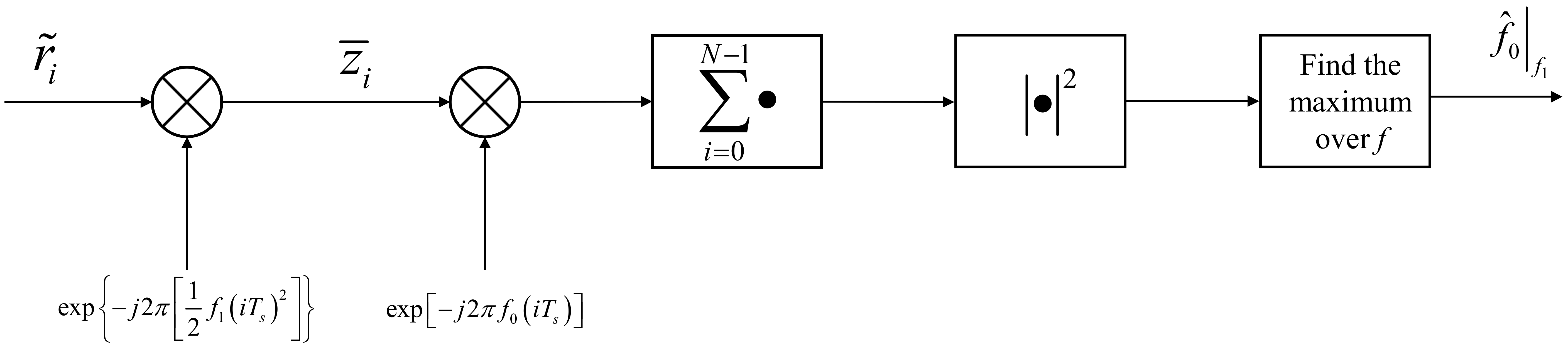
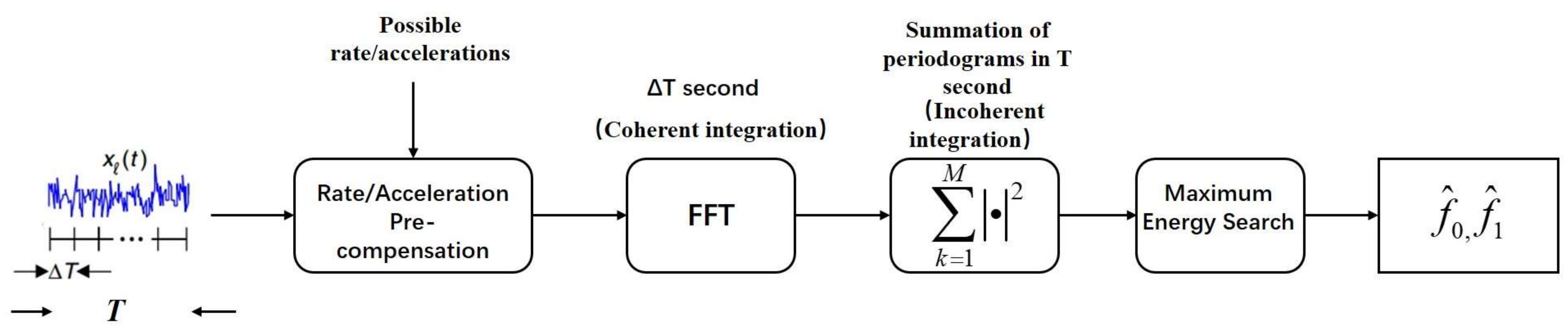
Although ML estimation does not designate which parameter should be estimated first, the given maximum energy search approach follows the interpretation that the raw signal samples are first compensated by a hypothesized Doppler dynamic phase model; then, the modified samples are used to make a periodogram estimation, as shown in Equation (13) [
12]:
If we use a second-order hypothesized Doppler dynamic phase model to compensate for the raw signal samples, then this approach is a two-dimensional (2D) maximum energy search. This is shown in
Figure 1 and
Figure 2.
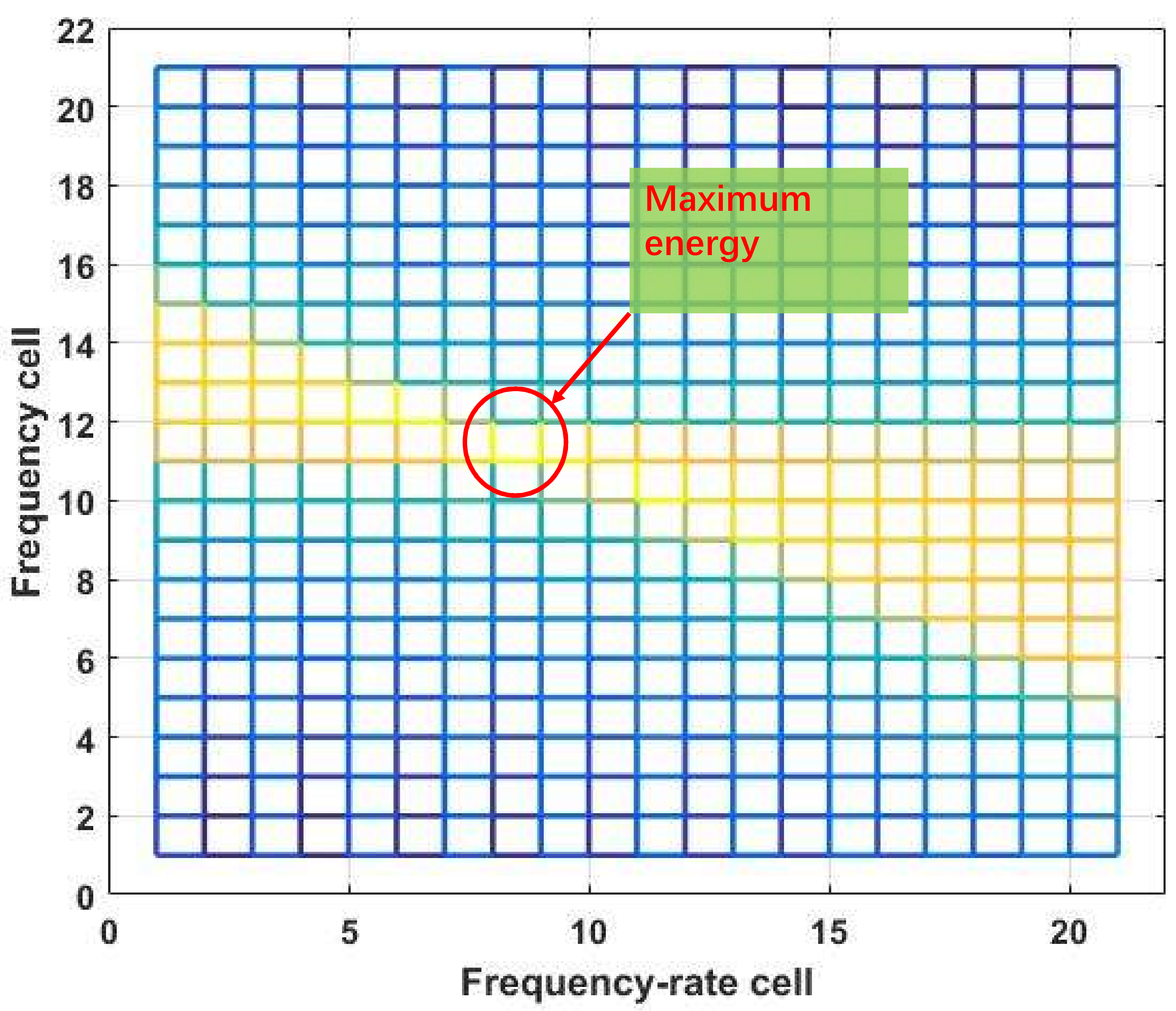
For each possible frequency rate value, the periodogram estimation is made, and the highest energy as well as the corresponding estimated frequency is selected for this frequency rate trial. After all the possible frequency rate trials have been made, a two-dimensional signal energy matrix has been acquired, within which the global maximum energy could be found, and the corresponding frequency index and the frequency rate index are the corresponding ML estimation values.
The 2D search approach is an open loop batch processing method. It computes the entire image of the signal for a given block of raw data, which allows immediate tracking recovery after a temporary signal loss [
21]. It also does not rely on any a priori information, and thus provides more robust tracking capabilities, although a priori Doppler dynamic phase information may help improve the estimation performance in the carrier estimation case [
14]. Besides, the 2D search approach tries to find the maximum energy among all the potential frequency cells, while Equation (13) could also be interpreted as:
which means that the maximum energy could also be searched among frequency rate cells, the second-order frequency rate cells, or there could be a joint search. When all of the Doppler parameters
have been correctly estimated and demodulated, the value of statistics
would equal to
N ×
A2. The estimation performance largely relies on the length of the coherent integration time, which corresponds to the raw signal sample numbers,
N. If a longer coherent integration could be made over something other than frequency cells, estimation performance may be improved.
Another potential factor that limits the 2D search approach is that its searching space is two-dimensional, which means that the chance that the energy of a noise-only frequency cell exceeds the energy of a signal-plus-noise frequency cell seems to be large. If the size of the searching space could be reduced, then the estimation performance may also be improved.
4. Performance and Simulation of 2D Maximum Energy Search Approach
As the 2D search approach is derived and practiced in EDL carrier detection and tracking for JPL (Jet Propulsion Laboratory)’s Mars explorations [
2,
3,
4,
5], we briefly review the carrier detection algorithm adopted in the past missions and the theoretical models used to evaluate the performance. Then, the discussion focuses on the selection of the processing parameters in the 2D search approach, and the influence of the processing parameters on the performance limitation. Finally, a simulation is made to evaluate the tracking performance based on the EDL trajectory of the MSL.
As described in JPL’s report, the 2D search approach is divided into a detection phase and tracking phase [
8,
14]. The difference is that all of the possible frequency cells and frequency rate cells trials are made among the full search space in the carrier detection phase, while in the carrier tracking phase, a local search is performed where signal parameter estimates from previous batches are used to reduce the search space for the current data batch. As the strategy on how to determine the local search space after previous estimates compensation needs more discussion, and we focus on the threshold performance of frequency estimation (meaning that the worst case is the most concern), the full signal parameter search space is considered as the common discussion baseline.
4.1. Algorithm Baseline and Theoretical Model
Following the introduction in Soriano and Satorius [
8,
14], the incoherent integration is used after the coherent summation in periodogram analysis to improve the carrier estimation performance. The carrier estimation algorithm (used for the direct carrier parameter estimation without using any previous information) is illustrated in
Figure 6.
The theoretical model of the carrier acquisition for the 2D maximum energy search approach is derived by Satorius, et al. [
14], and the basic functions are listed here for the following interpretation and comparison. The periodogram statistics is computed in Equation (15):
The statistic
is non-central chi square with 2M (
) degrees of freedom and the non-centrality parameter is
, provided that
l is the true carrier Doppler rate index and
fk is the true Doppler frequency. The standard probability density function for non-central chi square is shown in Equation (16):
where
is the modified Bessel function of the first kind, and of order
M − 1.
If
l does not agree with the true carrier Doppler rate index and/or
fk does not agree with the true Doppler frequency, the statistic
is central chi square with 2M degrees of freedom, and the corresponding probability density function is shown in Equation (17):
where
is the Gamma function, and the cumulative distribution function is denoted as
.
The carrier is correctly acquired provided that the associated statistics,
, is the largest one among the full search space (the detection threshold is set to 0 to maximize the acquisition possibility). So, the acquisition possibility is:
and the possibility of missed carrier acquisition is:
where
is the total cell number in the full 2D search space,
,
is the FFT cell number, and
is the Doppler rate cell number.
It could be seen that the carrier detection performance could be predicted using Equations (16)–(18), given the processing parameter value of FFT resolution (inverse to the coherent integration time ), the full incoherent time T (thus, the number of data segments for incoherent summation, M, could be computed by ), and the full Doppler (corresponding to ) and Doppler rate (corresponding to ) search range.
4.2. Selection of Processing Parameters
Among all of the processing parameters, the coherent integration time
and the full incoherent integration time
T play critical roles for the carrier detection performance. According to the recommendation from Soriano, et al. [
8], a rule of thumb for FFT resolution is that the maximum frequency change during the coherent interval in which the FFT is computed shall be smaller than a quarter of the FFT resolution, which leads to Equation (20):
The value of the incoherent integration time is decided according to the frequency deviation due to the second order Doppler rate not exceeding the length of the frequency cell, which could be written as Equation (21):
While the constraint for the incoherent integration time is obvious, the constraint for coherent integration time needs more investigation. According to the analysis by Graas, et al., [
21], the residual frequency dynamic would result in performance degradation in coherent summation. The influence of residual Doppler dynamics on energy loss in the coherent summation could be computed by the following coherence loss function [
12]:
where
,
, and
are the residual Doppler frequency, residual Doppler rate, and residual second-order Doppler rate, respectively.
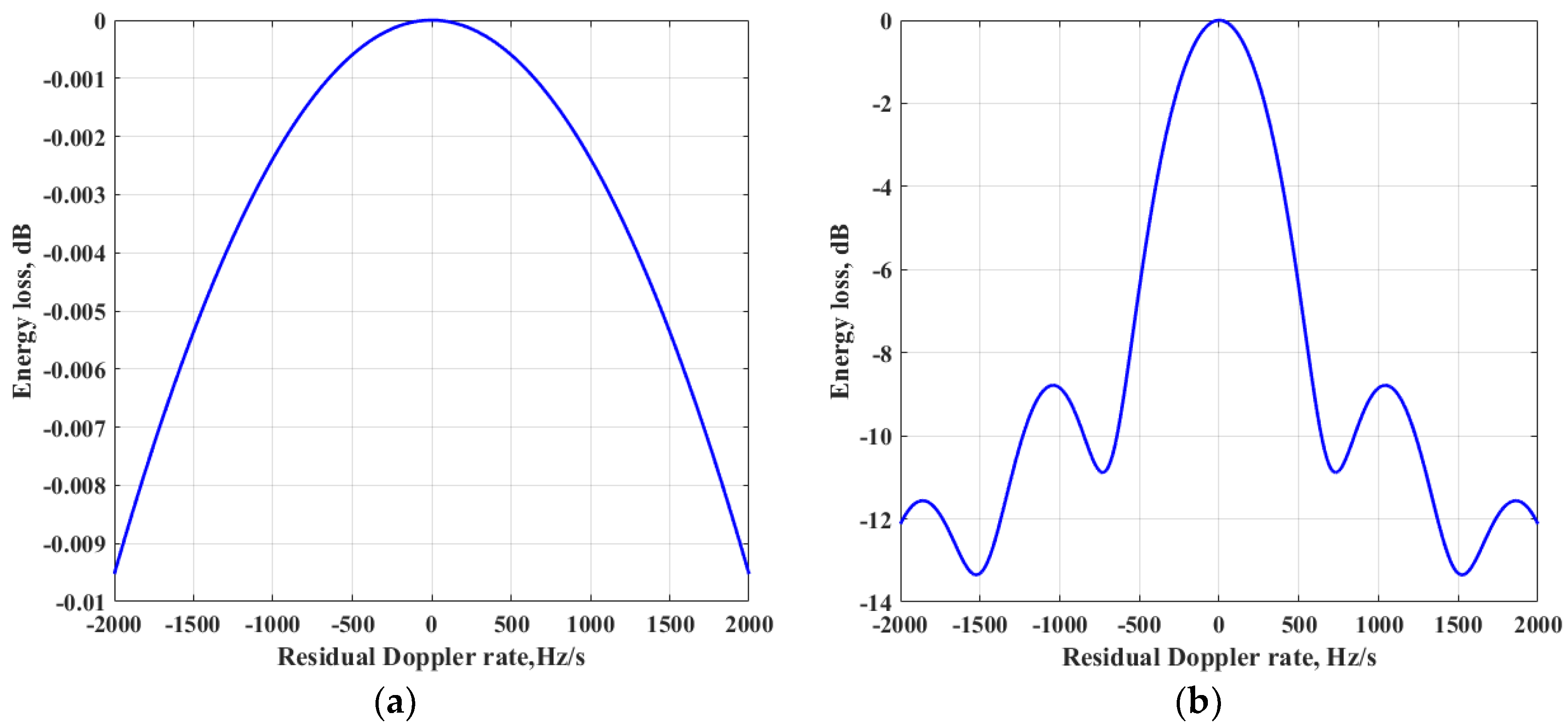
A numerical computation is made on Equation (23) to evaluate the influence of the residual Doppler rate. The complex sampling frequency is set to 200 kHz to cover the total Doppler frequency variation. The FFT resolutions are 10 Hz and 100 Hz, respectively. The energy loss due to the residual Doppler rate is plotted in
Figure 7.
As the coherent integration time increases from 0.01 to 0.1 s, the energy loss due to the 500 Hz/s residual Doppler rate increases from 0.0005 dB to about 6 dB, which is very significant. So, we take Equation (20) as the criteria to determine the FFT resolution.
4.3. Performance Analysis and Processing Parameter Influence Evaluation
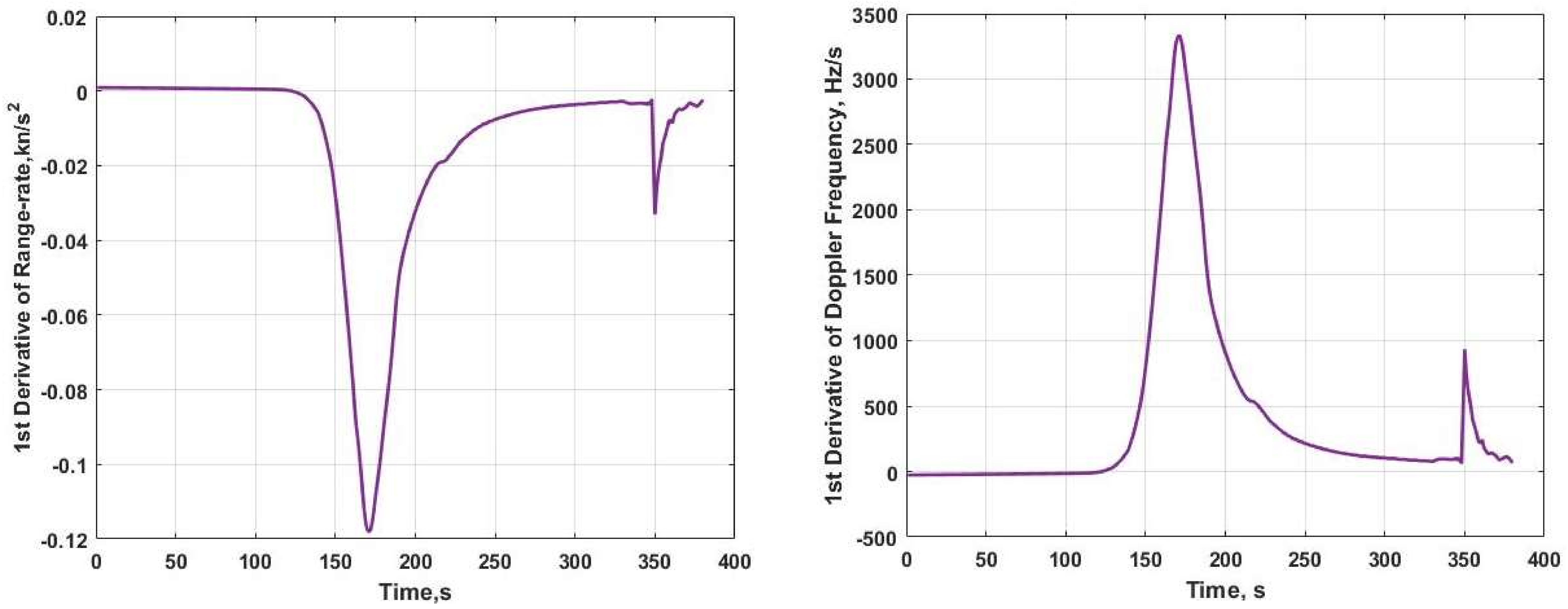
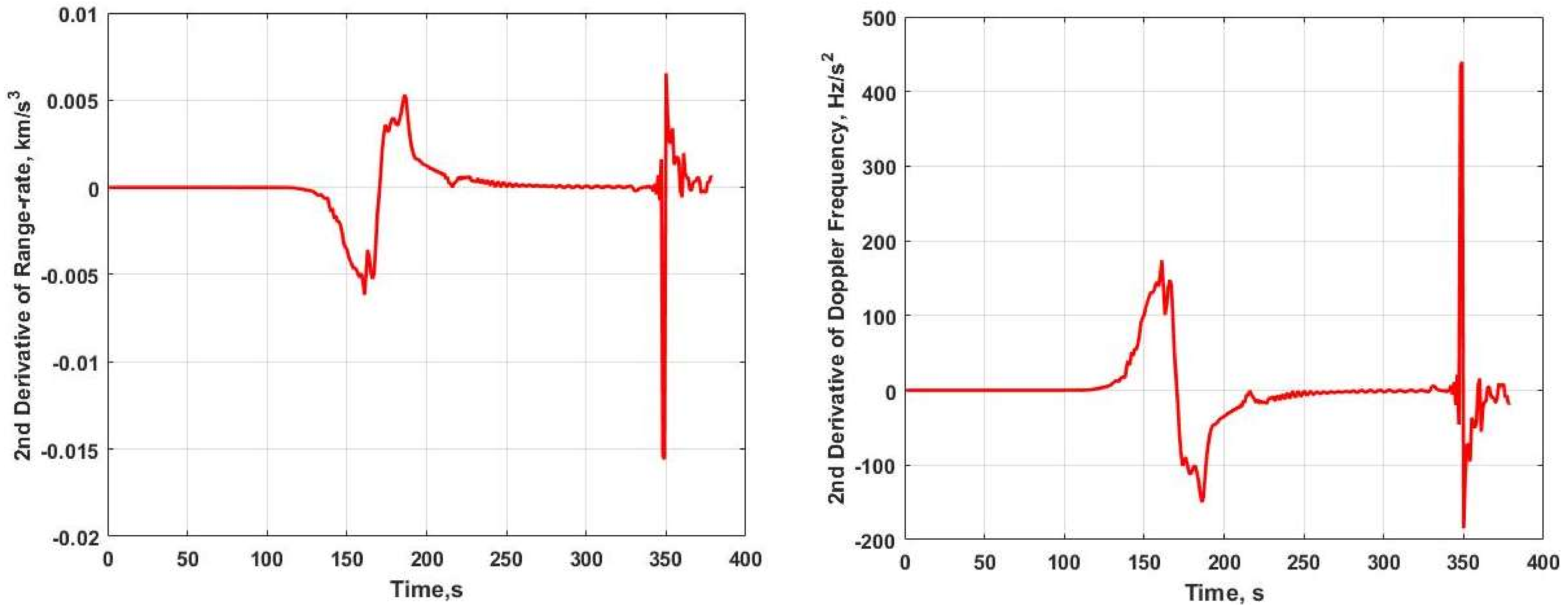
To make an evaluation and determine the estimation threshold of the 2D search approach, a simulation is implemented based on the EDL trajectory of MSL. Consider that the maximum Doppler rate is about 3400 Hz/s, and the second-order Doppler rate is about 440 Hz/s
2, the coherent integration time is set to 0.01 s, and the total incoherent integration time is set to 0.5 s for all of the EDL process parameter estimations. The detailed processing parameters are shown in
Table 1.
In the analysis shown in Soriano, et al. [
8], Doppler dynamics are varied with time, and different processing parameters are selected separately for the aerobraking flight phase and parachute deployment phase; this is a refinement processing of the raw data, and the performance could get better. In our analysis, we just use one set of the processing parameters to deal with the simulated data for the reason that the time instant when unfolding the parachute is not known in advance, as well as for analysis simplicity.
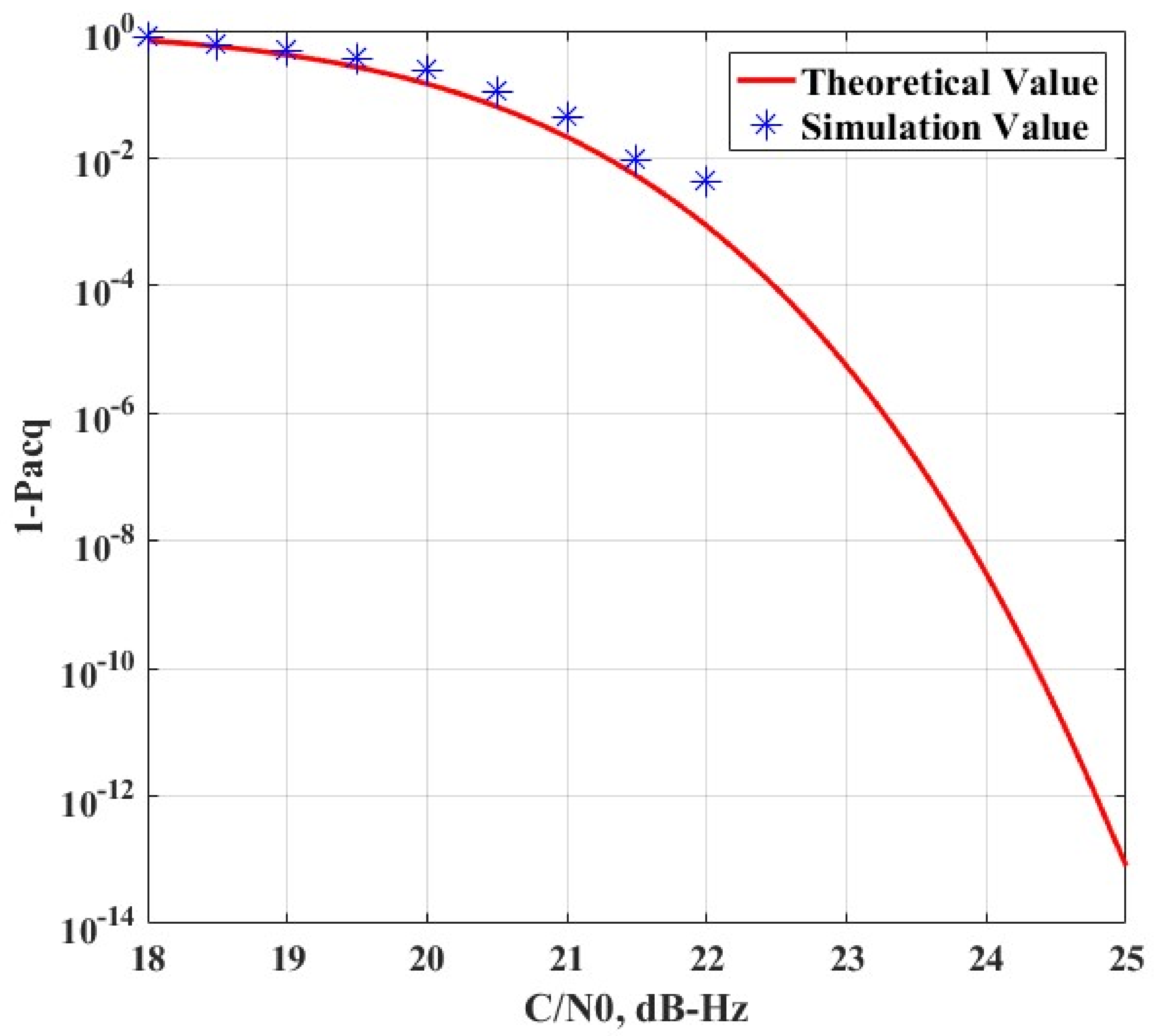
To evaluate the carrier detection performance, a simulation is made for different CNR based on the EDL trajectory of MSL. Five hundred trials are made for each CNR, and the probability of missed carrier acquisition in the simulation is counted and compared with the theoretical prediction computed from Equations (16)–(18), which is shown in
Figure 8. The simulated results are well consistent with the performance prediction, and the detection SNR for the selected processing parameters is about 22.5 dB/Hz. The large deviation of the simulation result from the prediction value when CNR is 22 dB/Hz is due to the limited simulation trials.
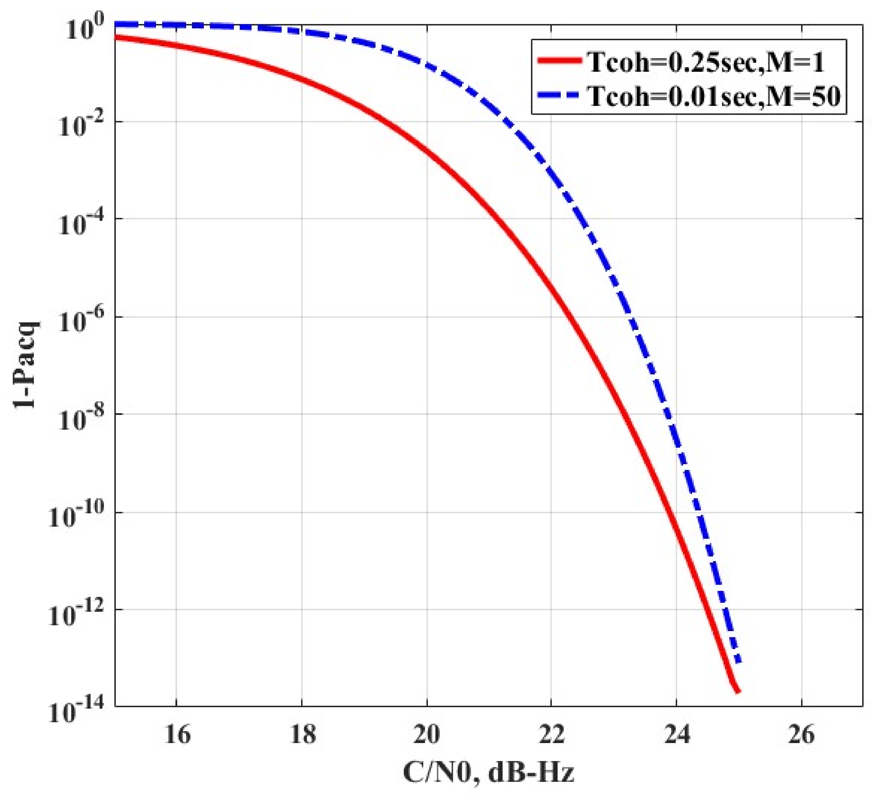
The influence of the coherent integration time and the incoherent integration time on the performance of carrier detection is different. The coherent integration is more efficient. As an illustration,
Figure 9 is a performance comparison of two integration approaches: the blue dotted line is 0.01 s of coherent integration with 50 blocks of incoherent summation, which corresponds to a total 0.5 s integration, while the red solid line is 0.25 s of coherent integration only. It could be seen that the 0.25-s integration has a better detection performance, although the first approach has an integration time of 0.5 s.
According to Equation (20), the main limitation of expanding the coherent integration is the existence of the large Doppler rate. Short coherent integration (corresponding to small FFT resolution,
) also leads to the inaccurate estimation of Doppler frequency, which in turn limits the carrier detection performance. Besides, as the complex sampling frequency is high (for example, 200 kHz), the sampling time is quite short (1/200 kHz = 5e
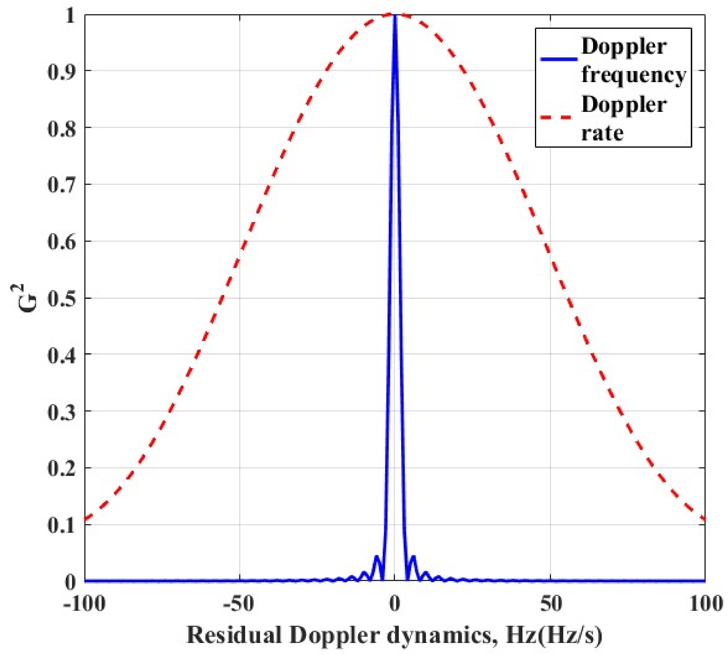
−6 s), and the time numerical contribution to residual phase due to residual Doppler frequency and residual Doppler rate is different in Equation (22). In mathematics:
when the residual Doppler frequency is numerically equal to the residual Doppler rate,
. Thus, the coherence loss function seems to be more tolerant with the residual Doppler rate than with residual Doppler frequency, which is shown in
Figure 10.
According to the above analysis, if the Doppler rate could be directly estimated and removed from the raw signal samples, the coherent integration time could be expanded, and a better frequency estimation performance may be acquired.
5. Performance and Simulations of Instantaneous Frequency Rate Tracking Approach
5.1. Basics of Cubic Phase Function and Squaring Loss Issue
The discrete-time cubic phase function (CPF) is defined by Equation (25) [
17]:
where
is the digitized raw signal samples,
m is the lag time,
K is an even number, and Ω is the frequency rate bin. The basic idea of the CPF is simple: folding up the raw data and making a cross-product followed by a summation results in the energy of the CPF concentrated along with the frequency rate law of the signal. Thus, the maximization of Equation (25) leads to a direct estimation of the instantaneous frequency rate (IFR) estimation.
As proved in the
Appendix A, the ML estimation of frequency rate for a linear chirp signal is shown in Equation (26); thus, the ML estimation of IFR could be obtained by Equation (27). According to the asymptotic properties of ML, the statistics to estimate IFR are asymptotically unbiased, and asymptotically attains the Cramer–Rao Lower Bound (CRLB).
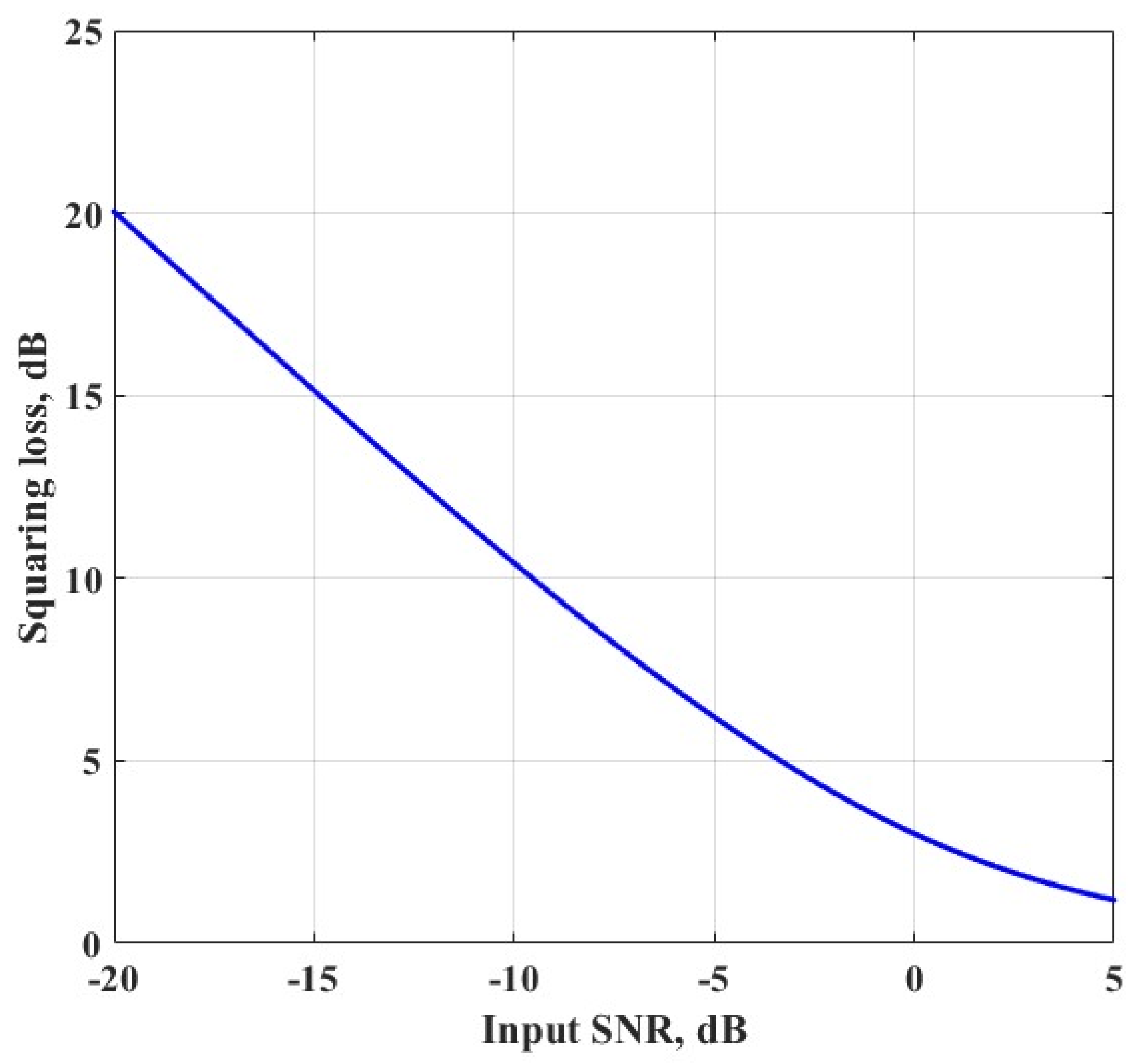
The main factor that limits the performance of the CPF estimator is the operation of cross-production. Cross-production helps cancel out the frequency term, leaving only the IFR term, but it also brings in the influence of squaring loss caused by the cross-production of thermal noise, which degrades the IFR tracking performance at a low SNR region.
The squaring loss could be computed by Equation (28), and the numerical value of squaring loss (SL) for each input SNR is shown in
Figure 11, which shows that the SL becomes significant when the input SNR decreases:
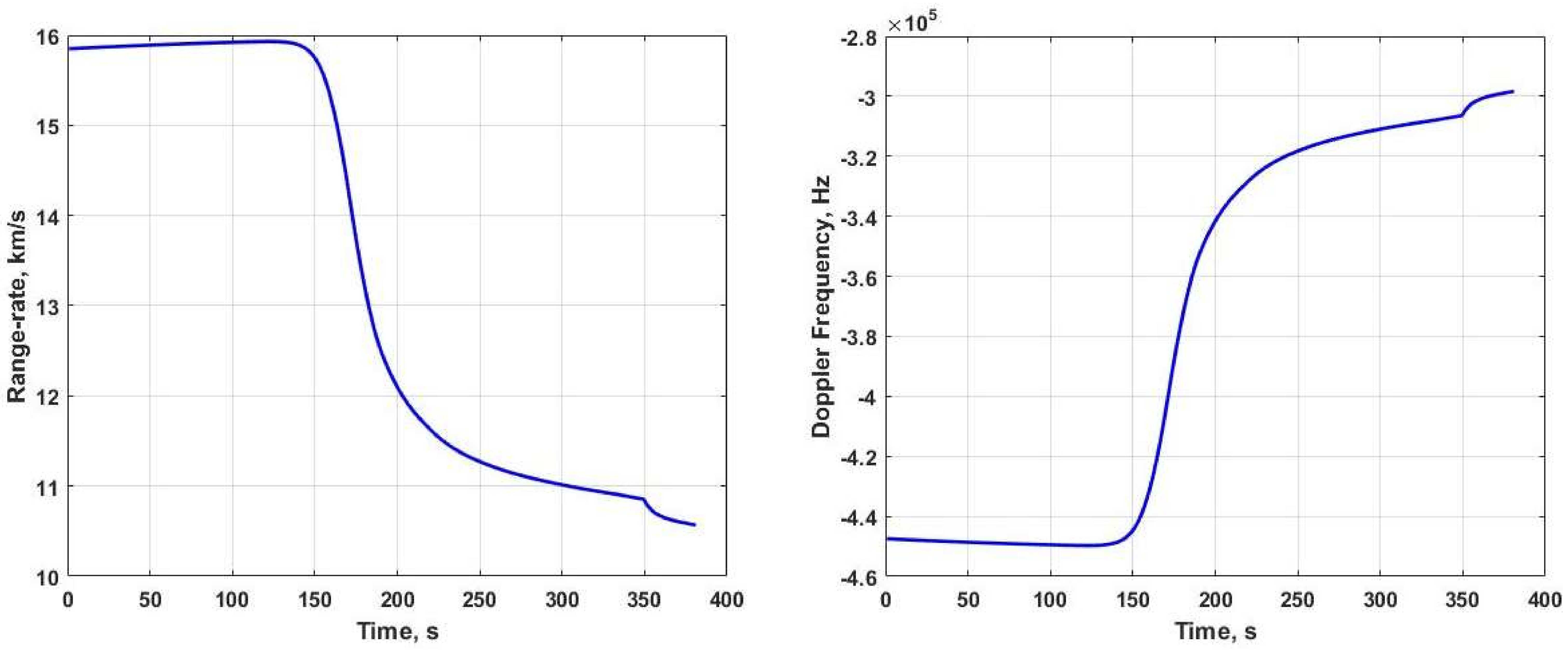
For the Mars EDL case, the Doppler drifts linearly with time when the spacecraft is approaching Mars, as shown in the first 100 s in
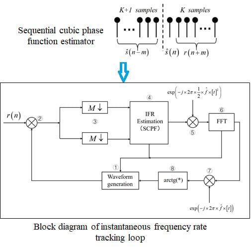
Figure 3. The Doppler dynamics is small, and the CNR of the received signal would be moderate or high. So, the Doppler phase of the received signal could be precisely reconstructed, which could be used as a priori Doppler phase information. We propose a sequential CPF (SCPF) estimator, which uses this information to eliminate the squaring loss effect in order to enhance the IFR tracking performance at a low SNR.
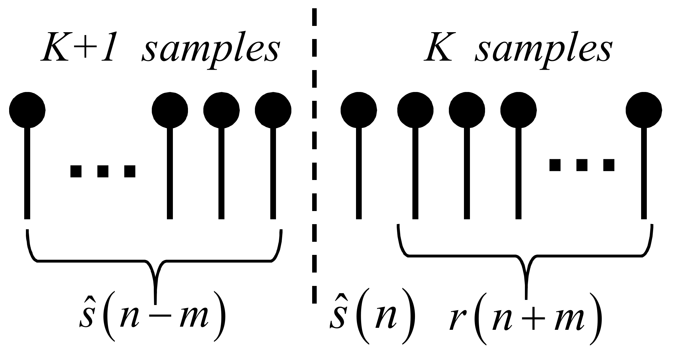
The SCPF statistics is computed by Equation (29). As shown in the equation, to cancel the frequency term,
K samples of
still come from the raw signal samples, while
K + 1 samples of
are generated from the previous parameter estimations. This process is illustrated in
Figure 12:
In each computation iteration of this sequential estimation manner, the IFR is first estimated using Equation (29), followed by the demodulation from the raw signal samples. Then, the frequency and initial phase are separately estimated using a ML estimator [
23]. Finally, a second-order phase model is generated using the estimated IFR, frequency, and the initial phase, and it is then used in the next computation iteration.
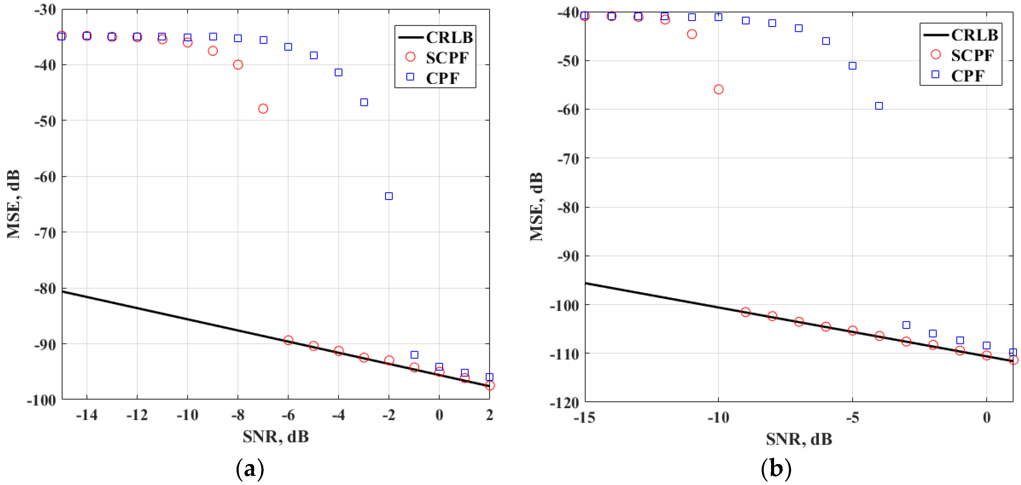
To evaluate the estimation performance of the proposed SCPF, the mean squared error (MSE) of the estimation at different SNRs is compared with the standard CPF, as well as CRLB. The CRLB of IFR in the digital domain is given by Equation (30) [
20]:
where
, and
is the complex sampling interval. It could be seen that the signal sample number
N greatly influences the variance of IFR.
Simulations for different sample numbers,
N, are implemented, and the results are shown in
Figure 13. It could be seen that the estimation threshold SNR decreases from −1 dB to −6 dB when
N is 201, and the estimation threshold SNR decreases from −3 dB to −9 dB when
N is 401. This proves that with the a priori phase model information, SCPF could accurately estimate IFR at a low SNR region, which obviously outperforms the standard CPF.
5.2. Detailed Estimation Algorithm
In this section, the full algorithm of the instantaneous frequency rate tracking approach is described in detail. First, we examine the search range of the IFR given the complex sampling frequency
Fs. CPF for a signal without noise is computed by Equation (31):
The above equation is maximized when:
Thus, when the search range of digital IFR
is
, the estimation range of
is:
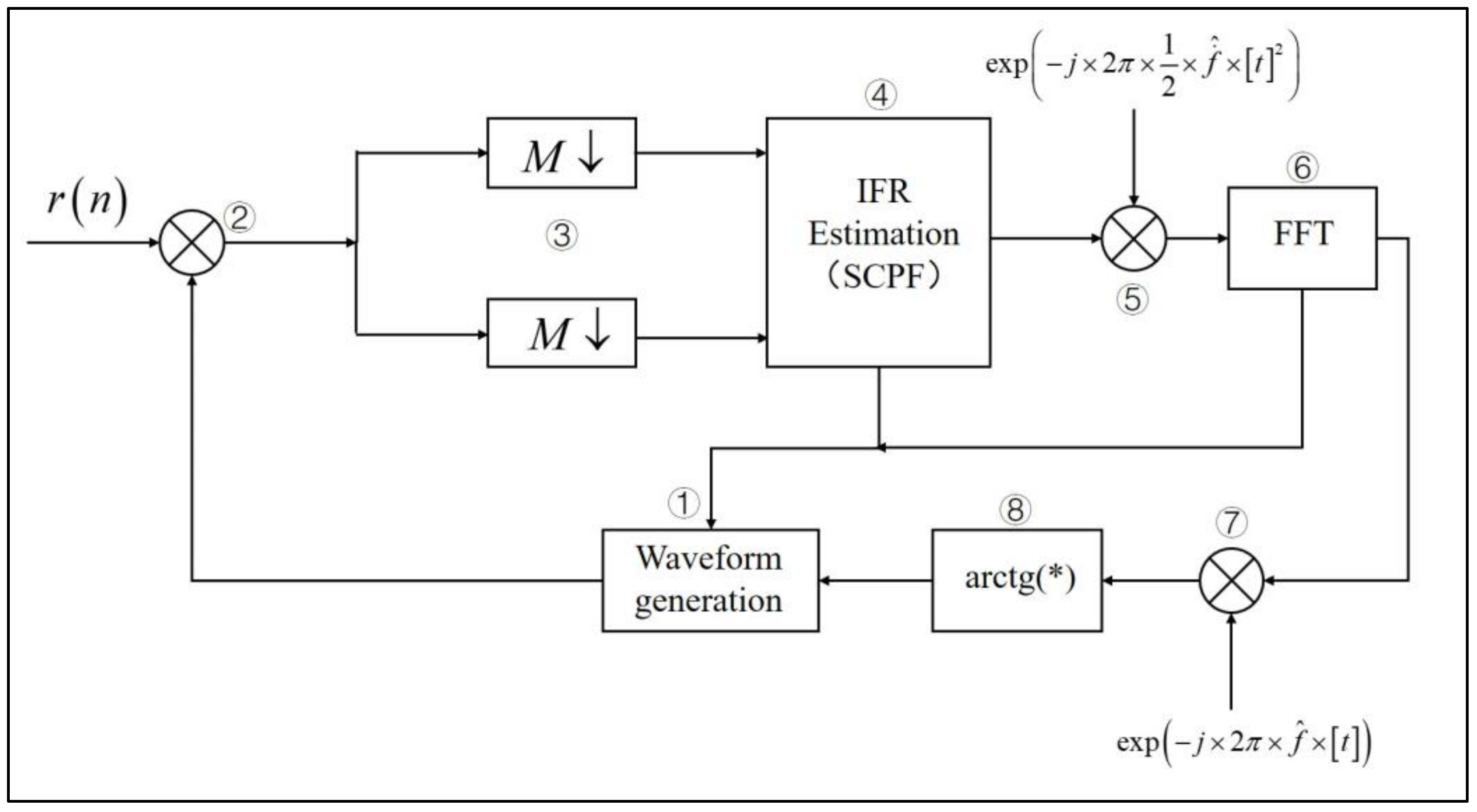
The block diagram of the IFR tracking approach is shown in
Figure 14.
The detailed description of the algorithm is as follows:
Step (1): Waveform generation
At label ① in
Figure 14, generate the second-order phase model from the previous estimation parameters using Equation (34):
where
,
, and
are the estimated phase, instantaneous Doppler frequency, and instantaneous Doppler rate in the previous computation iteration, respectively, and
is the corresponding time instant sequence shown in Equation (35):
and
K is the number of the total coherent integration samples.
The estimated waveform could be computed by Equation (36):
Note that the number of samples in the sequence is K + 1.
Step (2): Frequency cancellation
Construct the data sequence used for current estimation by combining
K + 1 samples of
and
K samples of
, where
come from the raw signal samples. As shown in
Figure 12, there are two subsequences which are dot multiplied with each other to cancel the frequency term. One sequence is called the forward direction subsequence
, and the other is called the backward direction subsequence
, which are defined in Equations (37) and (38), respectively:
Thus, the correlation sequence could be obtained by Equation (39):
Notice that at this step, the data rate is still equal to the complex sampling rate of the raw signal sample. As the sampling rate of the raw signal sample is usually several hundred kHz, the search range for IFR is also at this order of magnitude. The prediction analysis of EDL dynamics in
Section 3 shows that the maximum Doppler rate is no larger than 3.4 kHz/s; thus, the data rate could be reduced.
Step (3): Down-sampling
Down-sampling for the sequence
is realized by coherent summation. After down-sampling, the reduced rate complex data sequence is obtained, which is shown in Equations (40) and (41):
where
returns the real part of a complex number, and
returns the imaginary part.
M is defined by Equation (42):
and
is the data rate of the sequence
. The number of samples in
after down-sampling is
L.
Step (4)–IFR estimation
At this step, the ML estimation of instantaneous frequency rate could be obtained by Equation (43):
Step (5)–IFR demodulation
With the estimation value of IFR, the Doppler rate phase model could be generated by Equation (44):
where:
The IFR term could be demodulated from the raw signal samples by Equation (46):
Step (6)–IF estimation
At this step, the ML estimation of instantaneous frequency could be obtained by Equation (47):
Step (7)–IF demodulation
With the estimation value of IF, the Doppler phase model could be generated by Equation (48):
The IF term could be demodulated from
by Equation (49):
Step (8)–Phase estimation
At this step, the ML estimation of phase could be obtained by Equation (50):
Step (9)–Repeat to Step (1).
5.3. Selection of Processing Parameters
There are two important processing parameters in each computation iteration of the IFR tracking algorithm. One parameter is the data rate after the down-sampling processing, and the other is the integration time of each iteration. As there is no incoherent integration operation in the algorithm, the total integration time of each iteration equals to the coherent integration time.
For the data rate after down-sampling, the summation operation is after the frequency cancellation. This is similar to the processing manner in a digital phase locked loop (DPLL) [
24]. In a DPLL, a complex mixing operation is carried out between the incoming raw signal samples and the local predicted signal waveform samples, followed by a summation of the dot multiplied samples, which are used to generate the difference phase estimation between the incoming raw signal and the local predicted signal. In the IFR tracking algorithm, the summation of the dot-multiplied samples is used to estimate the instantaneous frequency rate, in contrast to the difference phase in a DPLL. There are two factors to be considered to determine the data rate
after down-sampling. One factor is the sample SNR after down-sampling, which could be computed by Equation (51):
which indicates that
should be as small as possible to improve the sample SNR.
The other factor is the search range for IFR, which is shown in Equation (33). Thus, the data rate could be selected by Equation (52), which maximizes the sample SNR and preserves the search range for IFR:
where
is the maximum value of the Doppler rate. Considering that the maximum Doppler rate is around 3400 Hz/s, the data rate
is selected to be 4 kHz.
For the integration time of each iteration, the main factor to be considered is the energy loss in the coherent summation due to a second-order Doppler rate. As there are two coherent summation operations in the IFR tracking approach, which are separately implemented to down-sample the samples after frequency cancellation and compute the SCPF statistics, the coherence loss function shown in Equation (53) is used again to evaluate the influence of the second Doppler rate:
where
N is the number of raw signal samples that are added together to generate a new signal sample after down-sampling,
L is the number of the signal samples that is used to compute the SCPF statistics,
, and
K is the total number of raw signal samples that are processed in each computation iteration of the IFR tracking approach.
Thus, the total coherent gain account for the influence of the second-order Doppler rate could be computed by Equation (55):
The whole EDL flight process consists of two independent parts: an aerobraking flight and parachute deployment. The characteristics of these two flight parts are quite different. In aerobraking flight, the Doppler and its derivatives’ curves vary with time smoothly, and the maximum value of the second-order Doppler rate is no larger than 200 Hz/s2. Meanwhile, the Doppler rate and second-order Doppler rate suffers an impulse dynamic when the parachute is deploying suddenly, and the maximum value of the second-order Doppler rate is no larger than 500 Hz/s2.
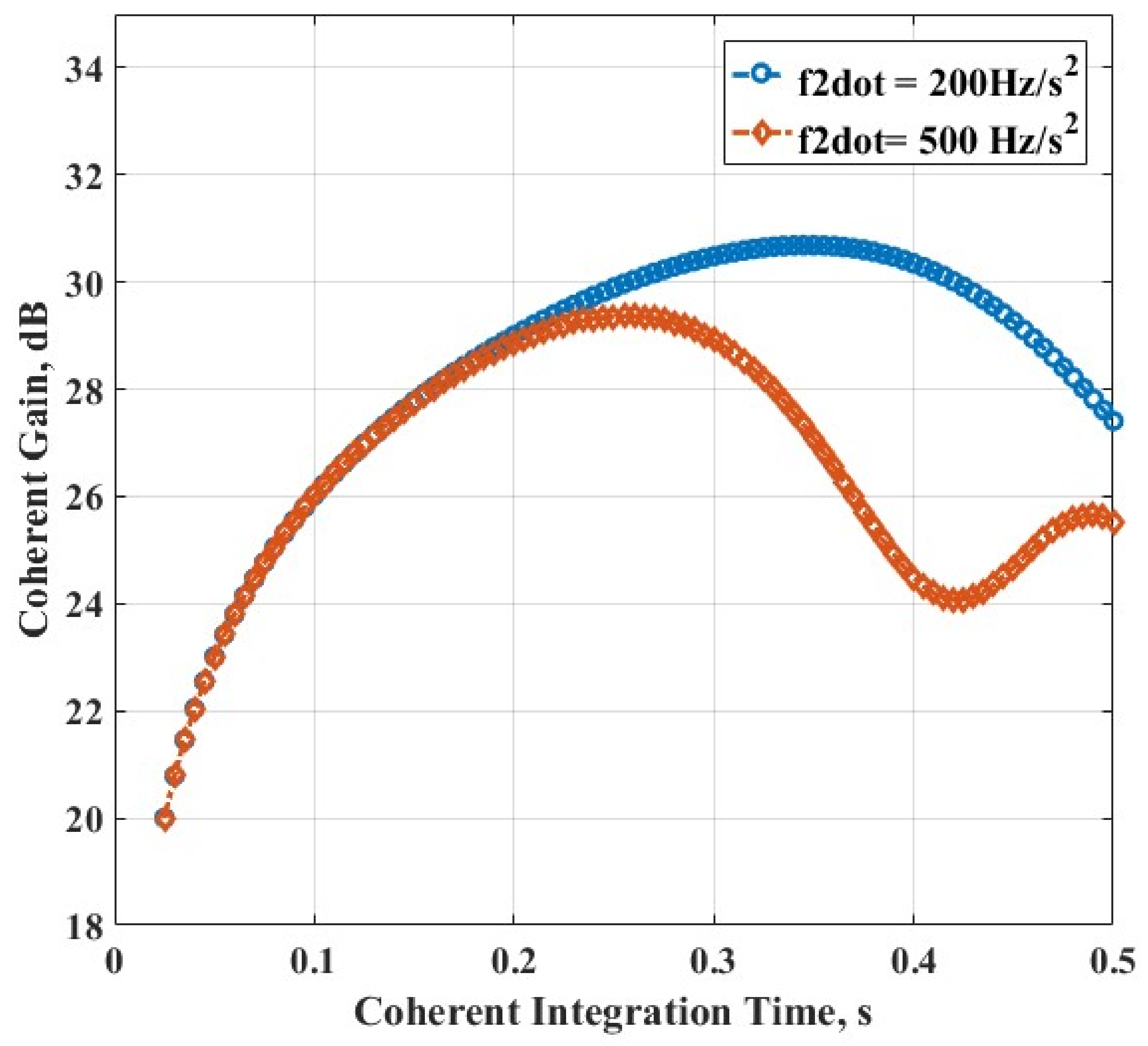
To evaluate the influence of the second-order Doppler rate, numerical computations are made for the coherence loss function based on Equation (55). The complex sampling frequency is 200 kHz, and the data rate is 4 kHz after down-sampling. The total coherent gain is plotted versus different coherent integration times, which is shown in
Figure 15.
As is seen in
Figure 15, the coherent gain gets to the maximum value of about 30.6 dB with 0.35 s of integration when the second-order Doppler rate is 200 Hz/s
2, and the coherent gain is about 30dB when the integration time decreases to 0.25 s. When the second-order Doppler rate is 500 Hz/s
2, the maximum of coherent gain is attained also with 0.25 s of integration. Thus, the coherent integration time is selected to be 0.25 s.
It should be noticed that the above analysis gives the theoretical foundation about the selection of integration time. If the time value exceeds the recommended value, the coherent gain will decrease. Besides, the dynamic response of the algorithm is also influenced by the coherent integration time, which still needs more investigation. In our processing approach, we use numerical simulations to evaluate the dynamic response of the algorithm given a certain data rate and coherent integration time.
5.4. Tracking Threshold Evaluation
According to the working mechanism of the IFR tracking approach, there are mainly two factors that greatly influence the performance. One factor lies at label ② in
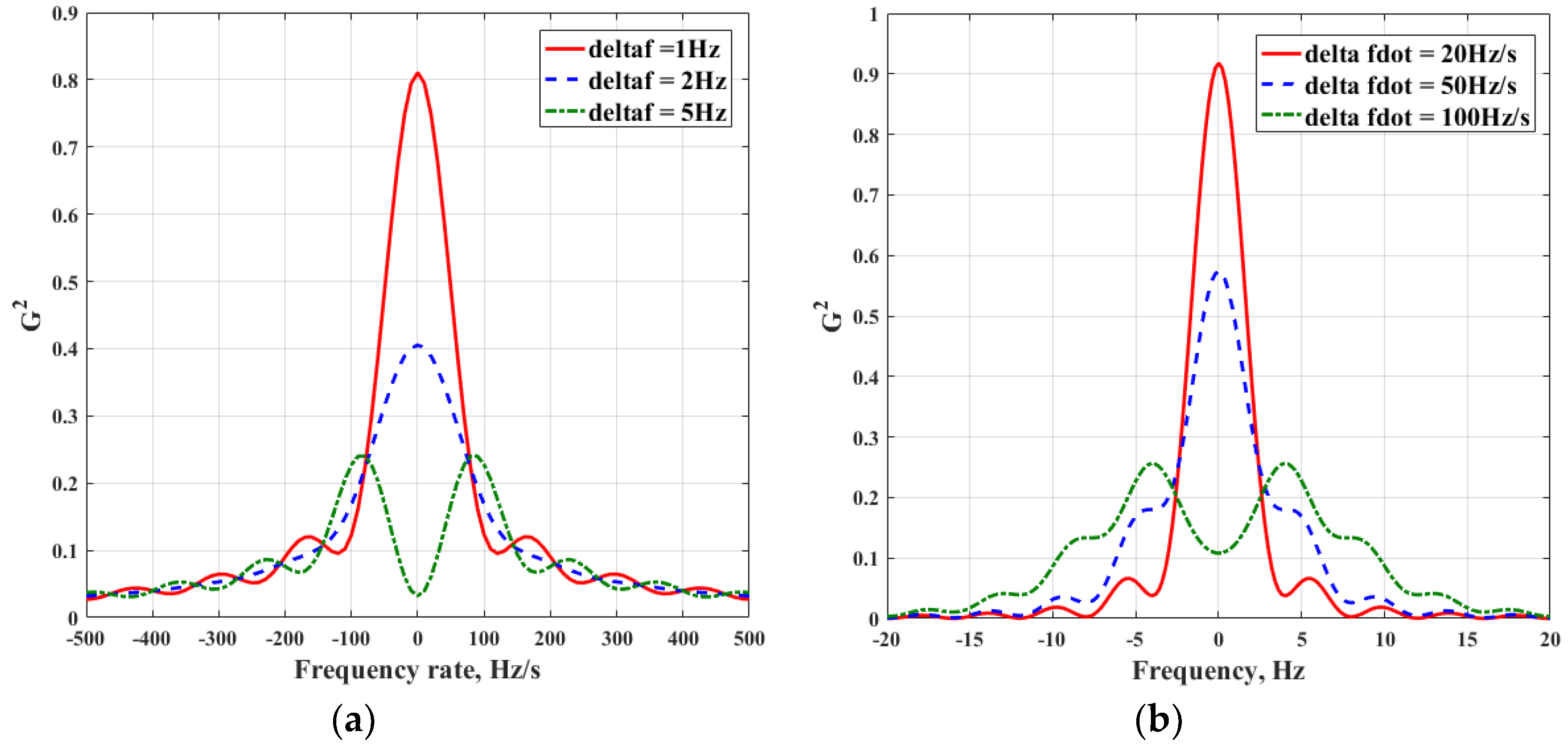
Figure 14, where the input raw signal samples are complex mixed with the waveform samples estimated in the last computation iteration. The frequency term is cancelled out, leaving only the frequency rate term to be estimated. If there is a mismatch of the instantaneous frequency between the input signal samples and the estimated waveform samples, the effect of residual frequency will arise, and the performance to estimate the IFR will be deteriorated. Another factor lies between labels ④ and ⑥. If the IFR is not estimated accurately enough, the estimation performance of frequency will also be influenced.
To numerically evaluate the two factors on tracking threshold, take Equation (22) again to compute the effects of residual frequency on the estimation of IFR, and the effects of the residual frequency rate on the estimation of frequency, which are shown in
Figure 16.
It could be seen from
Figure 16 that the residual frequency greatly influences the estimation performance of IFR. Although it does not introduce any estimation bias, the residual frequency degrades the signal energy severely. Two Hz of residual frequency leads to 4 dB (or
) in SNR degradation. As a comparison, the frequency estimation is more tolerant with the residual frequency rate, which is also shown in this figure. The residual frequency rate will not lead to a estimation bias for frequency, and a residual frequency rate of 50 Hz/s leads to only 2.4 dB (or
) in SNR degradation. Thus, a rule of thumb for determining the tracking threshold for the IFR tracking approach is Equation (56):
To theoretically compute the SNR for tracking threshold, the mean square errors (MSE) for frequency and frequency rate are laid out.
As shown by Li, et al. [
20], when the SNR is high, the CRLB for frequency and frequency rate estimation without outlier are as shown in Equations (57) and (58):
where SNR is the sample signal-to-noise ratio,
is the complex sampling interval, and
is the number of samples for parameters estimation.
When an outlier occurs, the estimation error variance could be found by assuming that each point within the search range has equal a priori probability of being chosen; thus, the frequency estimate may take on any value between
and
, and the frequency rate estimation may take on any value between
and
, and the corresponding variance could be computed by Equations (59) and (60):
According to the total probability formula, the lower bound for frequency estimation MSE is computed by Equation (61):
where
is the probability of correct frequency estimation.
Similarly, the lower bound for frequency rate estimation MSE is computed by Equation (62):
where
is the probability of correct frequency rate estimation.
Comprehensive simulations have been made to evaluate the tracking performance for the whole EDL flight. The results show that the theoretical analysis works well for the aerobraking flight, while for parachute deployment, the dynamic response of the algorithm behaves poorly when the coherent integration time is as large as 0.25 s. To improve the dynamic response of the algorithm, the integration time is reduced for parachute deployment. Thus, the tracking threshold is evaluated separately for aerobraking flight and parachute deployment.
5.4.1. Aerobraking Flight
Three groups of processing parameters are used in the simulation to evaluate tracking thresholds with different integration times. The detailed simulation parameters are shown in
Table 2.
The simulated probability of loss of lock for different integration times is shown in
Figure 17. The tracking threshold SNR for 0.15 s integration is about 25.2 dB/Hz, while for 0.2 s and 0.25 s integration, the threshold SNR is 23.6 dB/Hz and 22.6 dB/Hz, respectively.
As a comparison, the predicted RMSE (root of mean squared error) performance of the frequency and frequency rate for 0.15 s, 0.2 s, and 0.25 s of integration is computed by Equations (61) and (62), and plotted in
Figure 18, which seems to be consistent with the simulation results shown in
Figure 17. RCRLB is short for Root of Cramer–Rao Lower Bound.
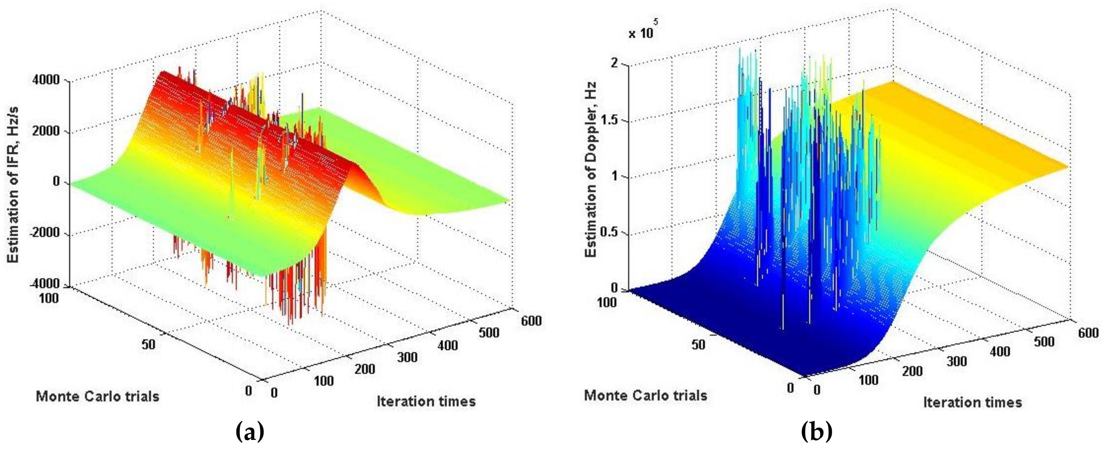
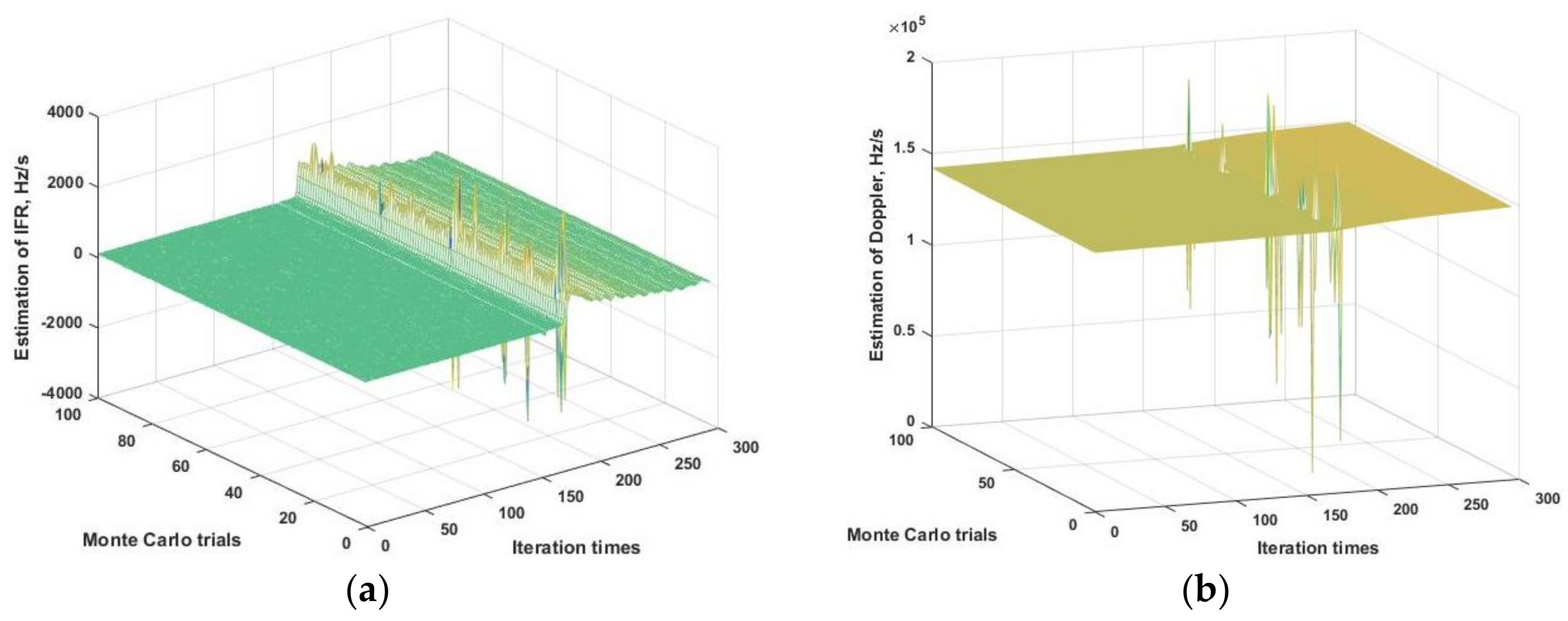
The simulation results of 100 trials for aerobraking flight with 22.6 dBHz and 21.8 dBHz CNR are separately shown in
Figure 19 and
Figure 20, respectively.
5.4.2. Parachute Deployment
For the parachute deployment mission phase, the Doppler rate and second-order Doppler rate are steady at the beginning. A sharp increase in each of the Doppler derivatives arise when the spacecraft is deploying the parachute, followed by a rapid declining in the Doppler dynamics. Thus, a good dynamic response of the algorithm is demanding to follow the rapid variation in the signal dynamics. According to
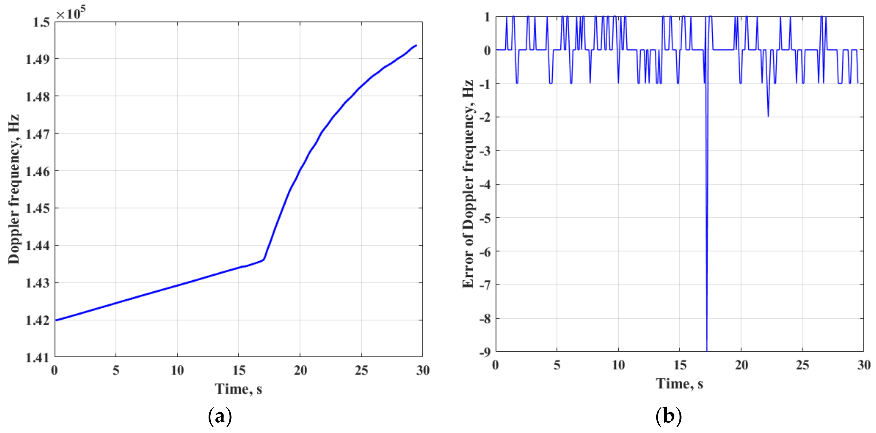
Figure 15, the integration time of 0.25 s is recommended for the maximization of coherent gain, while the dynamic response is quite limited for long integration time. Comprehensive simulations show that frequency estimation without any outlier could be obtained with 0.1 s of coherent integration, when the CNR is 29 dBHz. The corresponding estimation result is shown in
Figure 21.
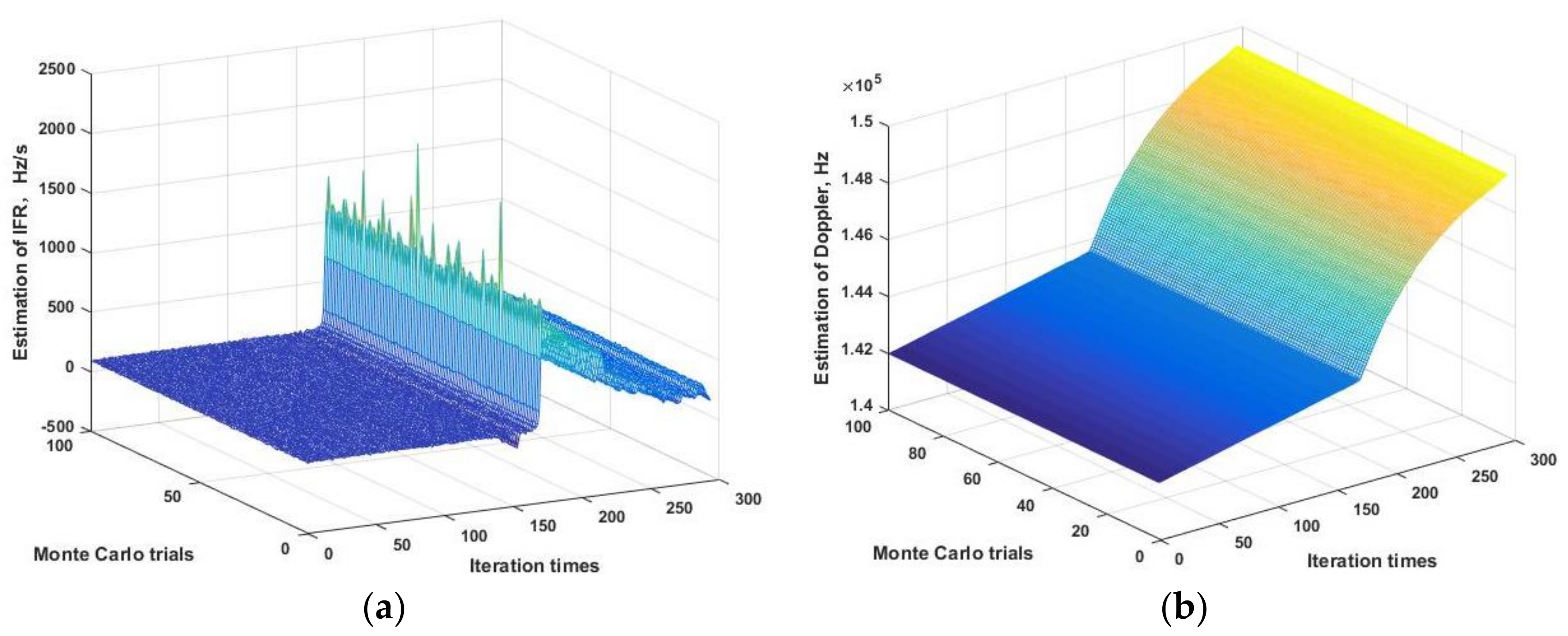
The simulation results of 100 trials for parachute deployment with 29 dB/Hz and 26 dB/Hz CNR are separately shown in
Figure 22 and
Figure 23.
6. Results and Discussion
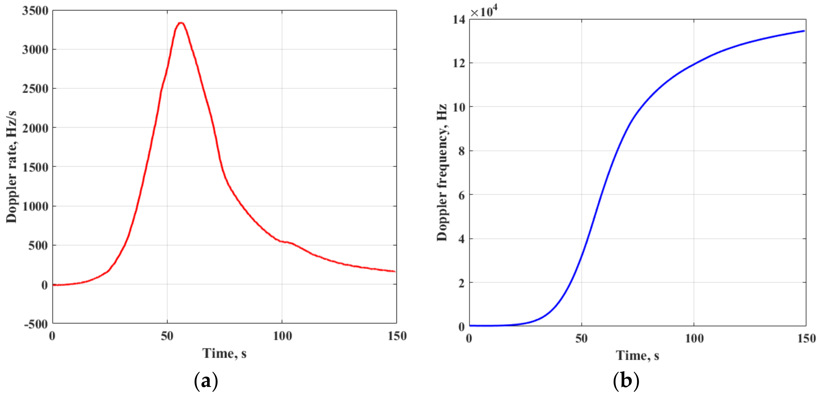
As the IFR tracking approach has a lower tracking threshold SNR for aerobraking flight, we first compare the carrier estimation performance for the two approaches. When the CNR is set to 22.6 dBHz, the Doppler and Doppler rate estimation results with an IFR estimation approach for aerobraking flight are shown in
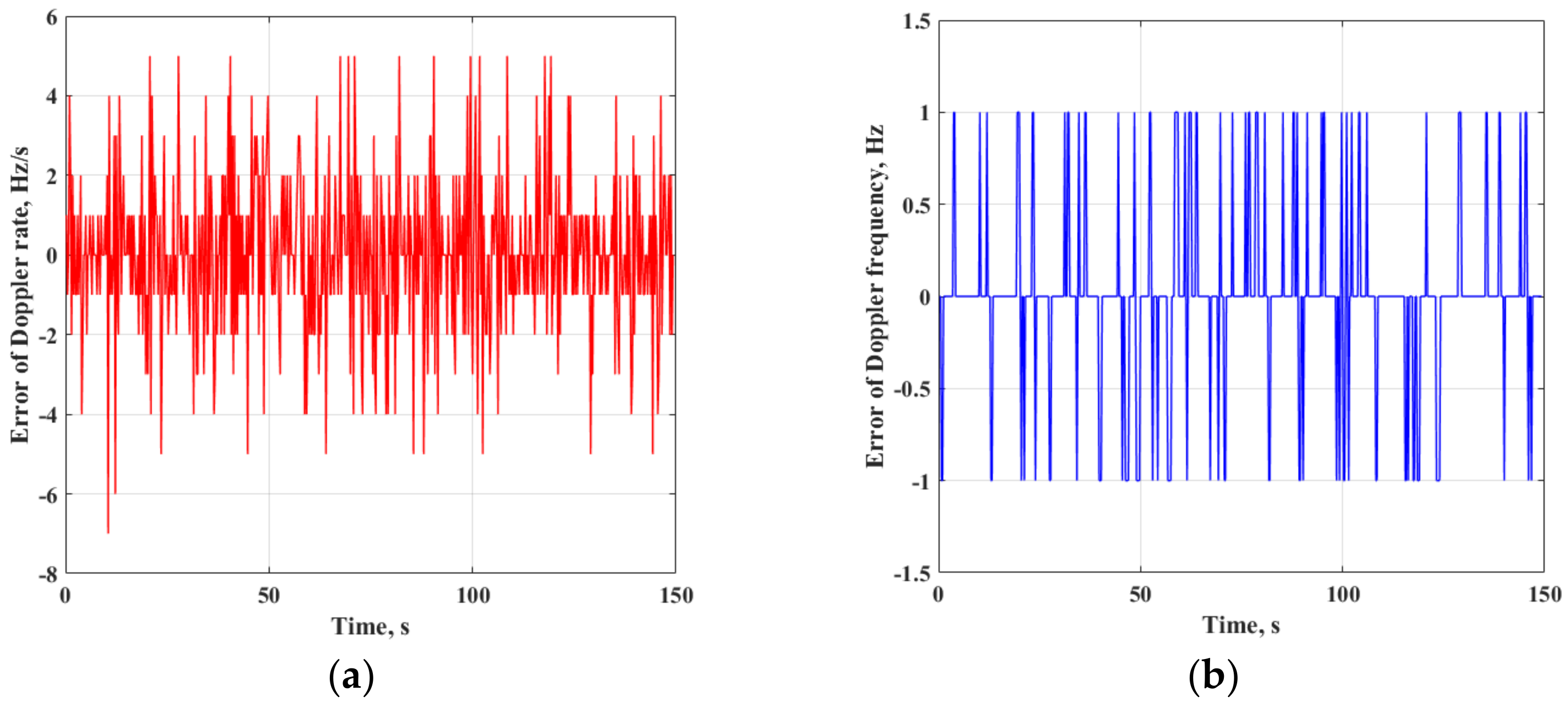
Figure 24, and the estimation errors are shown in
Figure 25.
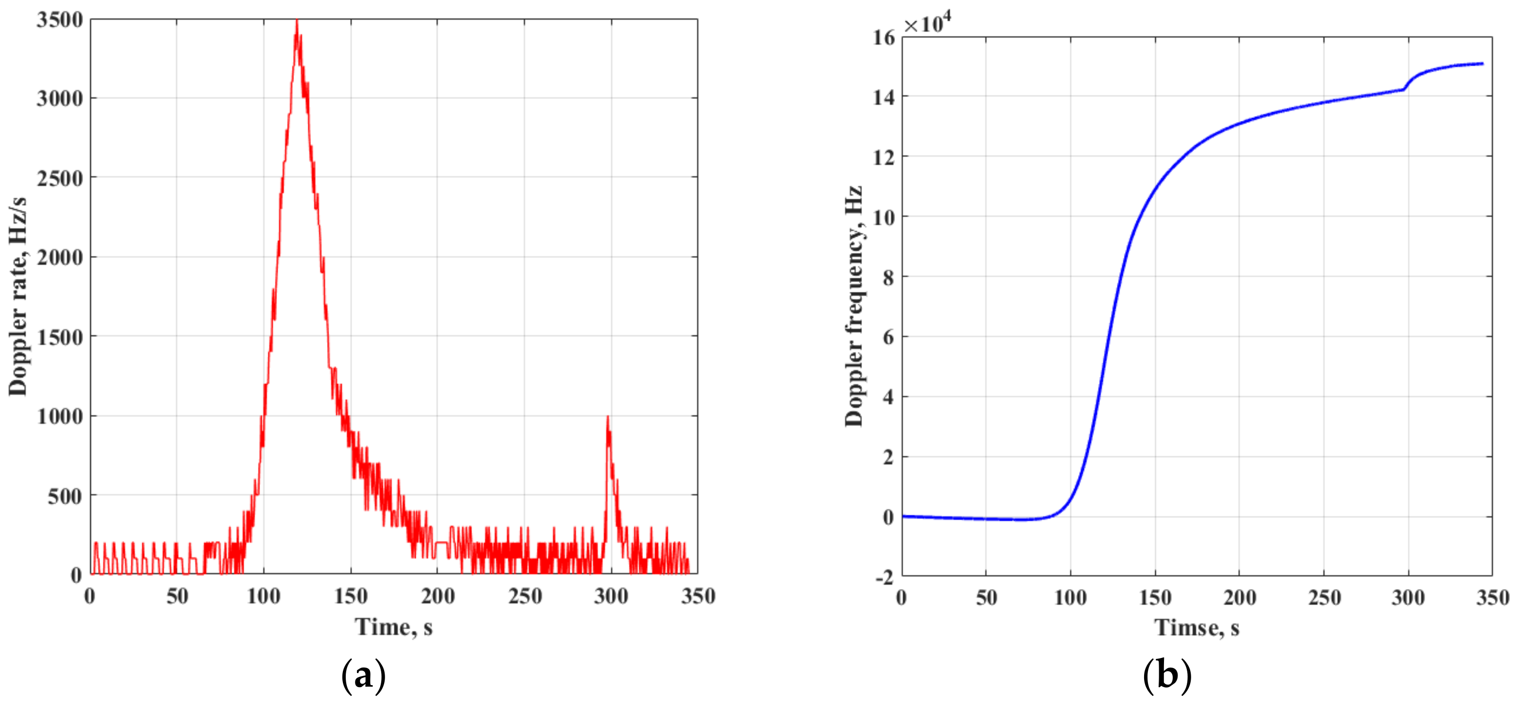
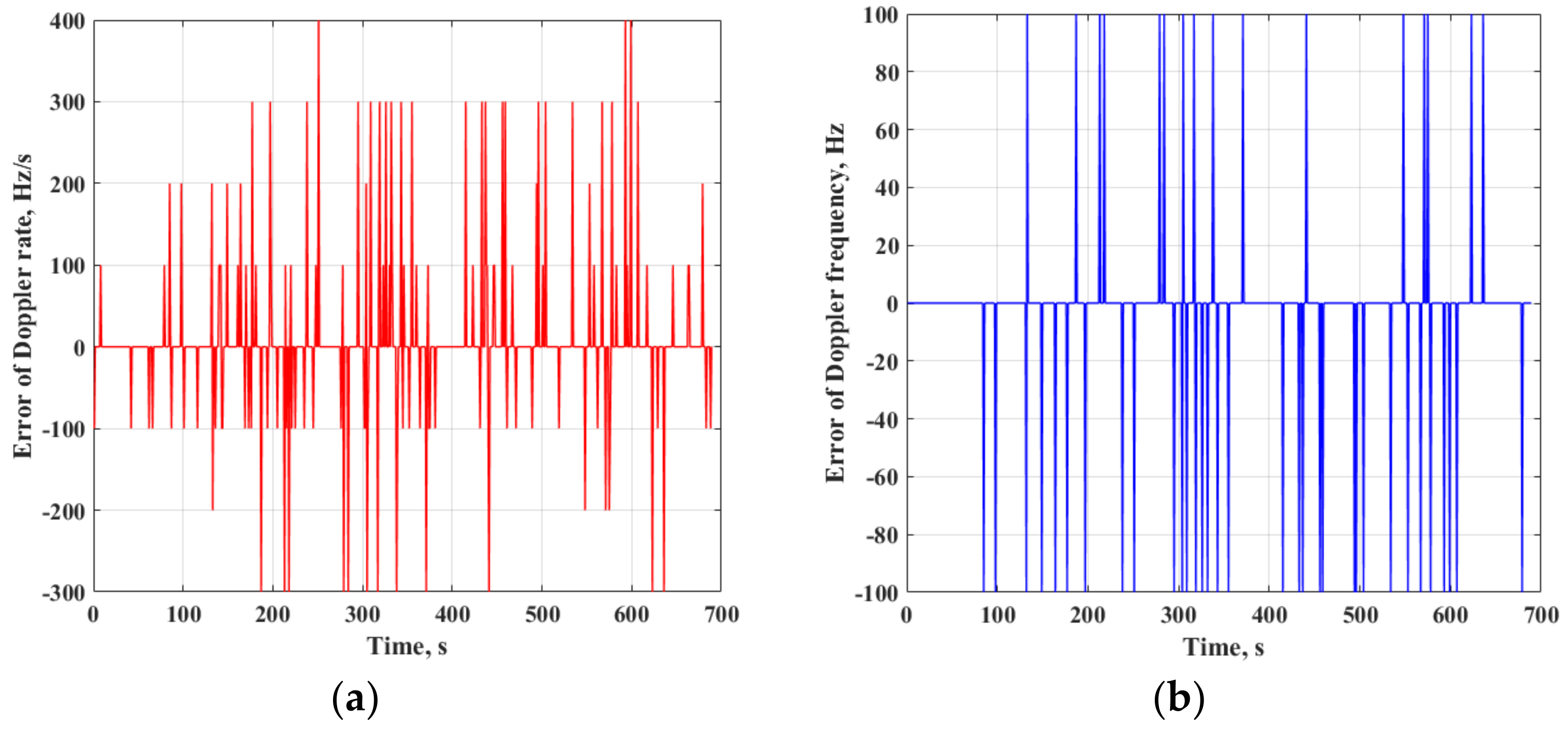
With a CNR of 23 dBHz, the Doppler and Doppler rate estimation results with a 2D search approach for the whole EDL flight are shown in
Figure 26, and the estimation errors are shown in
Figure 27.
The root mean square of the Doppler frequency and Doppler rate for the two approaches are summarized in
Table 3. With the help of direct instantaneous frequency rate estimation and the extending of the coherent integration time as long as possible, the r.m.s. for both Doppler frequency and Doppler rate have been largely reduced.
While the performance of IFR tracking approach is excellent, it does not work well for parachute deployment until the CNR goes above the tracking threshold, which is 29 dB/Hz with 0.1 s of coherent integration time. The RMS of Doppler frequency for an IFR tracking approach is 0.57 Hz, with an outlier only occurring at the time instant of parachute deployment, as shown in
Figure 21b. Another simulation shows that with the same CNR (29 dB/Hz), the RMS of Doppler frequency by a 2D search approach using the same value of processing parameters is 17.9 Hz, which indicates that the IFR tracking approach still has a better estimation performance.
On the other hand, the IFR tracking approach relies heavily on the a priori Doppler phase to engage the direct estimation of instantaneous frequency rate without squaring loss, and facilitate the extending of the coherent integration time, while the 2D search approach does not need any a priori information to estimate the signal parameters, and makes a decision on the detection of the signal presence. Thus, the 2D search approach, which is a standard open loop batch processing manner, has a better robust estimation performance. The threshold SNR is around 22.5 dB/Hz for the whole EDL flight, including the critical parachute deployment mission phase, while the IFR tracking approach could achieve a much more accurate estimation. In the practical approach, these two approaches could be combined to enhance the carrier tracking performance while still preserving an excellent performance of carrier detection when the signal is lost due to the brownout and blackout encountered in the Mars atmosphere EDL flight [
25].
The performance of both approaches could be improved by the reduction of parameter search space. For the signal parameters estimation in the Mars EDL case, the Doppler frequency and Doppler rate could be compensated by the designed nominal EDL trajectory if a good model of the Mars atmosphere and the thrusting forces onboard the spacecraft are available, or by the previous estimations, and the performance has been analyzed by Soriano, et al. [
8]. A similar operation could also be made on the IFR tracking approach, which may lead to a lower tracking threshold SNR. These works still need more investigation. The formal analyses in this paper try to evaluate the parameter estimation performance for the two approaches with no reduction of the parameter search space.
Another point that needs to be emphasized is that the a priori Doppler phase model is supposed to be generated from the carrier reconstruction by a third-order phase-locked loop when the spacecraft is approaching Mars. Further simulations have been made for the influence of the a priori phase model accuracy on the estimation performance of an IFR tracking approach. The results show that an IFR tracking approach is more tolerant with the uncertainty of the initial phase and frequency rate, while sensitive with the uncertainty of the frequency in the phase model. A rule of thumb for the initial frequency in the a priori phase model could also be selected as the deviation is smaller than 1Hz, which is not hard to satisfy when the downlink carrier is tracked by a third-order PLL at a moderate or high SNR.
7. Conclusions
This study has proposed a direct instantaneous frequency rate tracking approach to improve the carrier estimation performance in Mars entry, descent, and landing flight. The basic algorithm of the two-dimensional maximum energy search approach has been reviewed and reevaluated using the released Mars Science Laboratory EDL trajectory, and the discussion has been carried out on the selection of the processing parameter, which shows that the length of the coherent integration time is the most influential parameter, and the Doppler frequency rate caused by the trajectory dynamics is the main limiting factor. To extend the coherent integration time and improve the performance, the MLE based two-dimensional maximum energy joint search has been transformed to two groups of one-dimensional maximization problems, which separately estimate the instantaneous frequency rate and instantaneous frequency. As in the case of Mars EDL carrier reconstruction, in which a priori Doppler phase model with moderate accuracy is available, a sequential CPF estimator based on the sequential estimation manner is proposed to largely reduce the noise squaring loss issue, and the simulation results show that the SNR threshold of instantaneous frequency rate estimation by sequential CPF is reduced by 6 dB with respect to the standard CPF. The selection strategy of the processing parameters in the new algorithm has been analyzed in detail, and the simulation results show that the accuracy of carrier estimation has been improved by a factor of about 50 for the aerobraking flight in EDL at the same threshold SNR with the 2D search approach. Due to the high dynamics of the parachute deployment by the spacecraft, the coherent integration time has to be reduced for a better dynamic response, which leads to a higher threshold SNR than the 2D search approach, while the frequency estimation accuracy is still considerable if the lock could be maintained.
Considering the better performance of 2D search approach on robust estimation and free from a priori Doppler phase information, it is a possible direction for combining the two approaches to reconstruct the carrier in EDL flight precisely and firmly in future study.


