Machine Learning Using Hyperspectral Data Inaccurately Predicts Plant Traits Under Spatial Dependency

Abstract

Spectral, temporal and spatial dimensions are difficult to model together when predicting in situ plant traits from remote sensing data. Therefore, machine learning algorithms solely based on spectral dimensions are often used as predictors, even when there is a strong effect of spatial or temporal autocorrelation in the data. A significant reduction in prediction accuracy is expected when algorithms are trained using a sequence in space or time that is unlikely to be observed again. The ensuing inability to generalise creates a necessity for ground-truth data for every new area or period, provoking the propagation of “single-use” models. This study assesses the impact of spatial autocorrelation on the generalisation of plant trait models predicted with hyperspectral data. Leaf Area Index (LAI) data generated at increasing levels of spatial dependency are used to simulate hyperspectral data using Radiative Transfer Models. Machine learning regressions to predict LAI at different levels of spatial dependency are then tuned (determining the optimum model complexity) using cross-validation as well as the NOIS method. The results show that cross-validated prediction accuracy tends to be overestimated when spatial structures present in the training data are fitted (or learned) by the model.

1. Introduction

Remote sensing data from optical instruments are increasingly available and captured at a wide range of spectral resolutions and wavelength regions [1]. Sensors can be deployed on different platforms such as satellites, aircraft, drones or land-based vehicles [2]. Optical sensors capture spectral signals from a target surface but also capture spatial and temporal variations that are not necessarily targeted, regardless of the type of platform used [3]. Particularly reflectance captured from a continuous area is likely to exhibit significant spatial or temporal dependency for most types of surfaces [4,5]. Thus any biophysical or biochemical characteristic of vegetation estimated by remote sensing is expected to be affected by spatiotemporal autocorrelation, regardless of the type of environment, sensor, platform, spatial resolution, extent, period of collection, or sample design [6,7,8,9].

Many studies have demonstrated the feasibility to quantify plant traits, such as chlorophyll content, water content and leaf area index (LAI), at leaf and canopy level with satisfactory accuracy using remotely sensed data [10,11,12]. Applications for plant trait estimation range from assessing agricultural productivity and fire risk to monitoring biodiversity [13,14]. In most cases, explanatory variables based on narrow spectral bands from a comprehensive wavelength range generate models that more accurately predict plant traits than variables based on broad bands from visible spectra [10,15]. Therefore, hyperspectral data from either airborne or land-based platforms are often used to predict plant traits [2].

Despite the current knowledge of the physical relation between many plant traits and reflectance, it is still a challenge in a continuous and heterogeneous landscape, to consistently measure (or estimate) all factors needed to be able to use a deterministic model based on spectral radiance [16,17]. For example, even though the driving “cause-effect” relation between LAI and reflectance is known, data on other essential plant traits such as leaf structure, water content and leaf orientation are needed to be able to estimate LAI from reflectance data [18]. Consequently, most of the applications for estimating biochemical or biophysical characteristics of vegetation rely on empirical associations between reflectance and plant pigments or canopy structure [16]. Such empirical models must be trained with ground-truth measurements that are representative, in space and time, of the remote sensing data [19].

Ordinary least square regression using vegetation indices from a combination of two (or more) spectral bands is commonly used to predict plant traits. However, machine learning algorithms using the entire wavelength range, such as Partial Least Squares Regression (PLSR), Support Vector Machine (SVM), Random Forest (RF), or Artificial Neural Network (ANN) are often reported as being more accurate in predicting plant traits from hyperspectral data [3,20,21,22,23]. Using these supervised methods with a large set of predictors (i.e., the number of spectral bands) in relation to the number of observations is likely to cause model overfitting [24,25].

Overfitting occurs when the model incorporate random noises and data structures unrelated to the underlying relationship [26]. Therefore, models need to be constrained in their complexity to avoid overfitting. This is often achieved by limiting the number of terms or interactions used for learning data structures [27]. The procedure to select the optimum model complexity to reduce the risk of overfitting is called tuning [26]. Using a non-representative sample for training or using a sample from another population may jeopardise generalisation of a model. This could occur, for instance, when a model is applied to a new place or time that does not share similar characteristics [9,28].

A common way to estimate model generalisation or prediction accuracy is to estimate the Root Mean Squared Error (RMSE) of predictions based on a testing dataset that is kept separate from the sample set before the model is fitted. Alternatively, cross-validation techniques such as leave-one-out, k-fold subsetting or bootstrapping can be applied [26,29,30]. Despite being widely used, both approaches are based on subsets from the same sampling effort and may present unreliable estimations of model generalisation if the observations are spatially or temporally autocorrelated [9,31]. Little is known of how machine learning algorithms that are trained on hyperspectral data perform when predicting for a different but similar area or in a different timeframe without being retrained [3].

Spatiotemporal structures in remote sensing data may actually represent the spatial and temporal pattern and processes of the plant trait under study [6]. However, these structures may also present spatial patterns that are not causally related to the target plant trait. For example, soil characteristics or moisture content are likely to provoke changes in the spatial pattern captured by a sensor, either by altering a set of plant traits (targeted or not) or by capturing changes in the (soil) background [32].

For instance, using a field spectrometer it can be difficult to control variations in illumination geometry, canopy height and weather conditions across time and space under natural lighting [33]. Thus, the timing and order in which locations are visited to collect data can affect plant trait measurements, spectral measurements or both [34,35]. This aspect will be less apparent in satellite-based spectral data. However, taking in situ plant trait measurements may be so time-consuming that the vegetation gradually changes, possibly creating an undesirable data structure in the sampling collection [36,37].

Spectral, temporal and spatial dimensions are all serially correlated data. This means that there is a logical order in the data, where pairs of wavelengths, times or locations positioned nearby, are likely to be more similar than pairs coming from positions further apart [38]. While the spectral data provoke multicollinearity problems related to strong correlation among predictors in the model (bands), the other two might provoke autocorrelation within observations [39,40].

Spatial structures are often neglected, even when it is clear that the remote sensing data or in situ plant trait measurements are not far enough apart to be considered as spatially independent observations [13,21,41,42]. Autocorrelated observations violate the model assumption of independent and identically distributed observations (i.i.d) in ordinary regressions [5,43,44].

For many machine learning algorithms, explicit warnings about such assumptions are missing. However, noisy and autocorrelated data may cause model overfitting and misleading interpretations [6,25]. Often machine learning algorithms create latent variables to explain residual variance from previously fitted models in a progressive stepwise manner. Autocorrelation may not always be detectable in the residues of the final model [27].

Given the combination of (1) large numbers of correlated bands available in hyperspectral data relative to the number of observations, (2) plant trait measurements containing spatiotemporal structures, and (3) supervised model selection applied by machine learning algorithms: particular attention is needed when empirically estimating plant traits from hyperspectral data, to avoid fitting predictive models with a low capacity of generalisation.

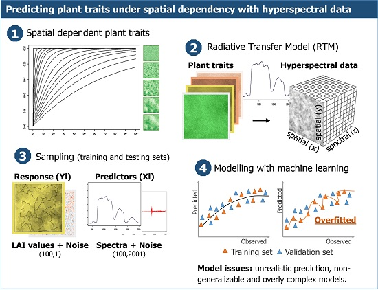
The objective of this study is to assess to what extent spatial autocorrelation in the landscape (and hence in the imagery) can affect prediction accuracy of plant traits when estimated by machine learning algorithms. The assessment focusses on prediction accuracy, model generalisation and independence of residuals across increasing levels of spatial dependency. The model fitting was implemented using two tuning processes, cross-validation and the NOIS method, which both aim to reduce the effects of overfitting while optimising model complexity. Machine learning algorithms are compared to less complex linear regressions using a vegetation index to assess model generalisation under spatial dependency.

2. Materials and Methods

Artificial landscapes were generated with increasing levels of spatial autocorrelation. This, in order to test the effect spatial dependency has on the accuracy of model prediction when using machine learning regressions based on hyperspectral data. The artificial landscapes generated are a hypothetical representation of vegetation with a short canopy (as in grassland). These landscapes were represented by layers of plant traits for further be used as parameters to simulate reflectance with Radiative Transfer Models (RTM).

Samples were drawn from the landscapes to train empirical models and to assess prediction accuracy while varying either the level of spatial dependency (autocorrelation ranges) or the spatial configuration (a unique realisation of a landscape).

The artificial landscapes were created by (1) generating variogram models with increasing ranges of spatial autocorrelation; (2) generating values for seven plant traits at a regular grid based on these variogram models using Sequential Gaussian Simulations of random fields (i.e., unconditional simulation); (3) simulating hyperspectral data using Radiative Transfer Models (RTM), as collected by spectrometers in the field, and (4) adding random and spatial dependent noise to the response variable (Y) and the hyperspectral data (X).

Of the seven plant traits generated, Leaf Area Index (LAI) was selected as the response variable to be predicted by the simulated hyperspectral data. LAI can be defined as half of the surface area of green leaves per unit of horizontal ground area [45]. This parameter was chosen since it is the primary descriptor of vegetation functioning and structure, and essential to understanding biophysical processes [35].

2.1. Simulating Plant Traits

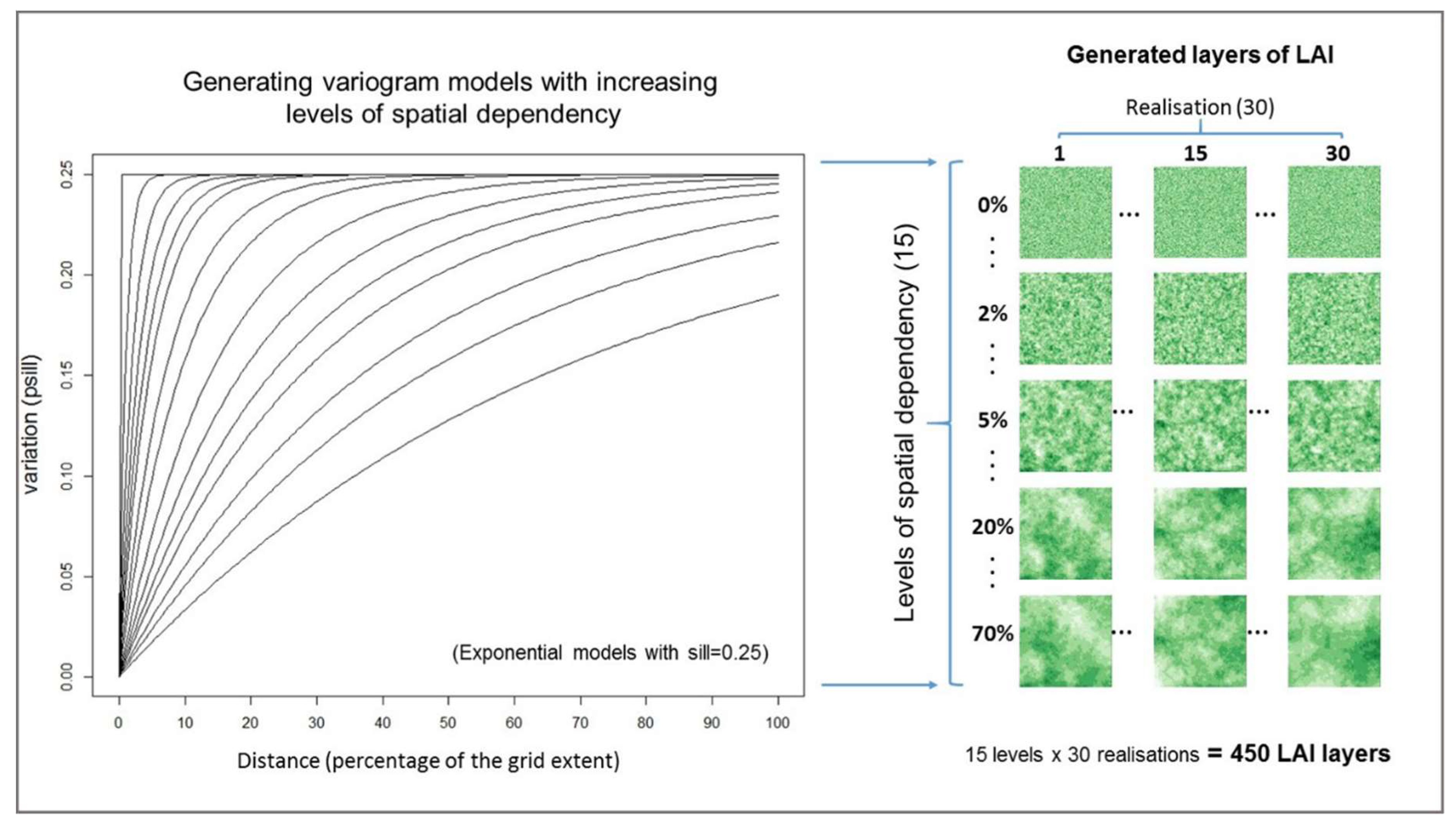
Unconditional simulations, based on variogram models, were used to generate plant traits representing landscapes with different levels of spatial dependency at a regular grid of 100 by 100 cells. In total, 15 levels of spatial dependency were created with autocorrelation ranging from zero to 70% of the extent of the artificial landscape (Figure 1). In other words, the landscapes ranged from ones where all pixels were independent in space to landscapes with autocorrelation of up to seventy percent of the grid extent.

Thirty realisations of each plant trait layer were generated for each of the 15 levels of spatial dependency. Each realisation used a single random path (neighbourhood selection) through the grid locations to create a unique spatial configuration [46]. The spatial patterning of a plant trait layer from the same realisation will be more similar between following ranges of spatial autocorrelation than between different realisations of the same range of autocorrelation. This is illustrated in Figure 1, where patterns are more similar along the vertical lines than along horizontal lines. Initially, 450 LAI layers were generated, corresponding to 30 different realisations for each of the 15 levels of spatial dependency (30 × 15). The levels of spatial dependency were selected to produce similar intervals between variograms curves (Figure 1), rather than a scale equally spaced by distance or percentage of the area extent.

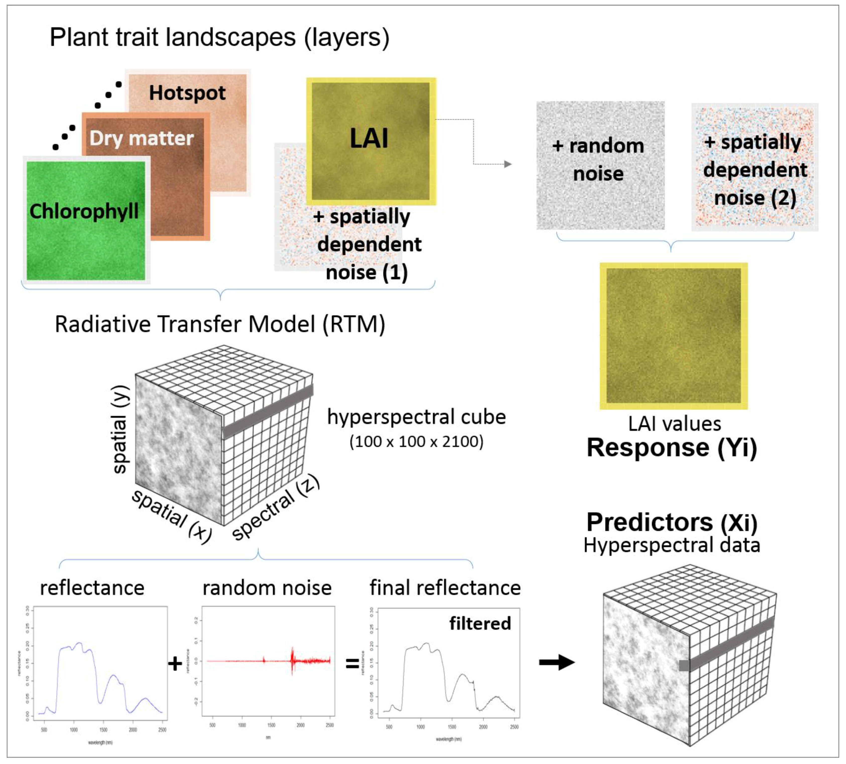
Layers of plant traits were also generated based on Chlorophyll Leaf Content (Cab), Leaf Structure (N), Dry Matter Content (Cm) and Hotspot (hspot) to be used as input in a Radiative Transfer Model (RTM; PROSAIL 5B, see 2.2). The plant traits Carotenoid (Car) and Water Content (CW) were, based on their strong correlation with other plant traits, as applied by Vohland and Jarmer (2008) [47] and Jarocińska (2014) [48], defined as a function of Chlorophyll (Car = Cab/5) and of dry matter content (Cw = 4/Cm⁻¹), respectively.

The resultant 450 layers per plant trait were rescaled to present the same mean and standard deviation across realisations and levels of spatial dependency as presented in the

Table 1. PROSAIL parameters used to simulate canopy reflectance for each 450 landscapes combination.

	Parameter	Description (unit)	Distribution	R2 with LAI
Leaf	Cab1	Chlorophyll a+b concentration (ug/cm2)	~N(28,4.5)	0.36
	Car2	Carotenoid concentration (ug/cm2)	~N(5,0.7)	0.35
	Cbrown3	Brown pigment (unitless)	0	-
	Cm1	Dry matter content (g/cm−2)	~N(0.004, 0.0005)	0.69
	Cw2	Equivalent water thickness (cm)	~N(0.016, 0.002)	0.66
	N1	Leaf structure parameter (unitless)	~N(1.5, 0.12)	0.48
Canopy	LAI1	Leaf Area Index (unitless)	~N(3.1, 0.6)	-
	hspot1	Hotspot parameter (unitless)	~N(0.05, 0.01)	0.50
	LAD3	Leaf angle distribution (attribute)	Erectophile (90°)	-
	psoil3	Dry/Wet soil factor (unitless)	0	-
Geometry	tto4	View zenith angle—VZA (degree)	~U(0,5)	-
	tts4	Solar zenith angle—SZA (degree)	~U(30, 38)	-
	psi4	Relative azimuth angle (degree)	~U(0,360)-U(129,252)	-

¹ simulated from plant traits by levels of spatial dependency and rescaled to present a Normal distribution ~N (mean, standard deviation). ² a function of another parameter: Car = Cab/5 and Cw = 4/Cm⁻¹. ³ fixed values for all landscapes. ⁴ generated randomly from a uniform distribution with max and min ~U(min,max), varying according to hypothetical in situ measurements using a field spectrometer: where tto is the deviation from nadir (0°); tts = 90° minus the max and min sun altitude, and psi = ~U(0,360) minus the max and min solar zenith angle during the collection.

. Each plant trait layer was rescaled using the equation:

$${\mathrm{Trait}}_{\mathrm{rescale}}{=\mathsf{\mu }}_{\mathrm{trait}}+\frac{{(\mathrm{x}}_{\mathrm{i}}-{\overline{\mathrm{x}}}_{\mathrm{layer}}{)\mathsf{\sigma }}_{\mathrm{trait}}}{{\mathrm{s}}_{\mathrm{layer}}},$$

(1)

where:

• ${\mathsf{\mu }}_{\mathrm{trait}}$ and ${\mathsf{\sigma }}_{\mathrm{trait}}$ are the mean and the standard deviation of the plan trait as defined in Table 1;
• $x_i$ is the plant trait value of the pixel $i$, for $i$ = 1, 2, …, 10,000;
• ${\overline{x}}_{layer}$ and $s_{layer}$ are the mean and standard deviation of the 10,000 simulated values of the layer.

This procedure standardised the data distribution while retaining the original spatial autocorrelation and spatial configuration. Random variations were then added to each plant trait layer (except LAI) to avoid linear combinations between parameters as all traits were generated from the same set of variogram models and realisation seeds. The random values added to each pixel of the generated plant trait layers followed a normal distribution with mean zero and standard deviation according to the scale of the variable and the assumed coefficient of determination (R²) with LAI (Table 1). These procedures guaranteed that the correlation between a trait and LAI was kept almost constant for all levels of spatial dependency and the different realisations considered. The R² with LAI was defined based on experiments found in the literature [49,50].

2.2 Simulating Spectra

A Radiative Transfer Model (RTM) was used to simulate 450 hyperspectral cubes. The PROSAIL 5B model was adopted to simulate wavelengths from 400 nm to 2500 nm with a 1 nm spectral resolution, generating in total 2100 bands. This physical model used 13 parameters divided into leaf, canopy and observation geometry properties [18,51]. The model parameters were set to simulate spectra from grassland landscapes captured by a field spectrometer [52].

Besides the seven leaf and canopy plant traits described before, three other RTM parameters were included (Table 1). These three were kept at fixed levels: Brown pigment (Cbrown) = 0, assuming that the canopies are entirely green; Leaf Angle Distribution (LAD) = Erectophile or 90°, given that is the principal orientation observed on grassland; and the soil moisture factor (psoil) = 0, assuming that moisture has no influence across space. The last three parameters in Table 1, related to illumination and observation geometry, were randomly generated from a uniform distribution ~U(min,max), varying solar and view angles slightly based on the hypothetical sample collection using a field spectrometer under natural light conditions.

2.3. Adding Variability into the Simulations

As RTM models are fully deterministic, different kinds of noise were added into the data to represent variations expected when observations are collected sequentially (rather than simultaneously) and by different instruments (spectra and ground-truth). It is unlikely that hyperspectral data captured by a handheld spectrometer will present the same spatial structures observed on the LAI values measured with another instrument (e.g., LAI2200). For this reason, the random and spatially dependent noise was added separately to the spectra and to the LAI values that were used as the response variable in the training set (Figure 2). Before generating spectral cubes, spatially dependent noise N~(0, 0.25) was added to all LAI layers, using the same spatial dependency, but from a different realisation.

Random noise per waveband was also added to the spectra from a normal distribution with mean and standard deviation as estimated in a pilot experiment. This was done, because, when capturing spectra under natural light conditions, random variations in reflectance will occur as a result of the sensitivity of the sensor for specific regions of wavelengths. An experiment with a portable spectroradiometer (ASD FieldSpec® 3, Boulder, CO, USA) was conducted to estimate the magnitude of such expected random noise per band. The spectra from 40 distinct grassland surfaces were captured in similar atmospheric conditions. Each plot was measured for 30 consecutive times from spectral ranges between 400 nm and 2500 nm under natural sunlight around noon with a clear sky in summer.

As some wavelengths were strongly affected by the random noise, smoothing with a Savitzky–Golay filter was applied over a length of 11 bands [53]. A spatially dependent noise of N~(0,0.1) was also added to the LAI layers before extracting data sets for model selection and validation, but with a different realisation than the ones used for simulating spectra. Random noise N~(0,0.1) was also added to create the final 450 LAI layers to be used as response variable (Figure 2).

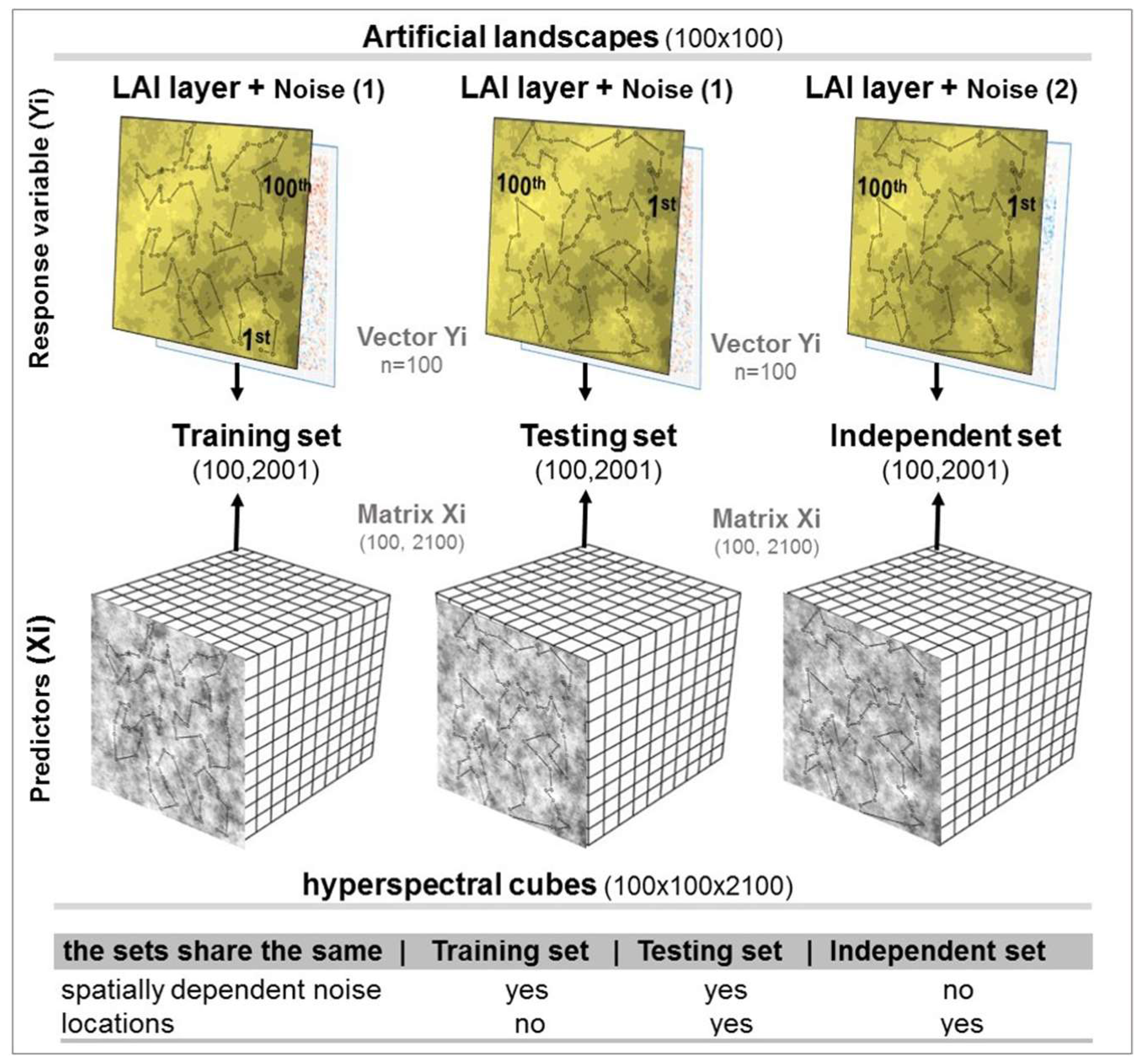
2.4. Sampling Schemes

Observations were extracted from the simulated spectral cubes and the final LAI layers to train empirical models (training set) at a hundred random x and y positions. At another hundred random locations, observations were extracted to validate the fitted models. This second set of locations was used for extracting two validation sets: a testing set and an independent set. The testing set is extracted from the same artificial landscapes (i.e., same realisation and spatial dependency) as the training set, but with different values of random noise. The independent set contains both different, random and spatially dependent noise. The intention is to mimic an independent test set collected from the same landscape but in a different sampling campaign. In this case, the spatially dependent noise captured by one campaign may not match the other one used for training the model.

A path that minimises the distance travelled to collect these random points was defined for the two distinct sets of sample locations (Figure 3). The LAI and reflectance values were stored in this sequence of sample collection to train models, and later, to assess the presence of spatial correlation in the residues. The average distance between two consecutive points of the path was approximately 8% of the total extent of landscapes for both training and testing sets. There is an exclusive set of sample locations (training and testing) for each of the 30 realisations to reduce the risk of a particular sample distribution randomly selected causing a strong influence in the analyses.

2.5 Modelling and Performance Assessment

Partial Least Squared Regression (PLSR) and Support Vector Machine (SVM) were selected as machine learning algorithms in this study because these are frequently used for modelling hyperspectral data, and their prediction accuracies have been reported as high, relative to other algorithms [21,54]. Also, these techniques have the capacity to deal with multicollinearity and high dimensional data. Overfitting can be reduced by limiting the level of complexity of these models, such as the number of components in PLSR.

Two tuning methods were applied to select model complexity: traditional cross-validation and a novel method called Naïve Overfitting Index Selection (NOIS) [25]. When tuning a model with cross-validation (we used 10-fold cross-validation), a model is selected with a complexity that minimises the Root Mean Squared Error (RMSE) of the predictions from the validation subsets [24]. This procedure was randomly repeated ten times, resulting in a combination of 100 subsets of training and validation sets from the original data [26]. 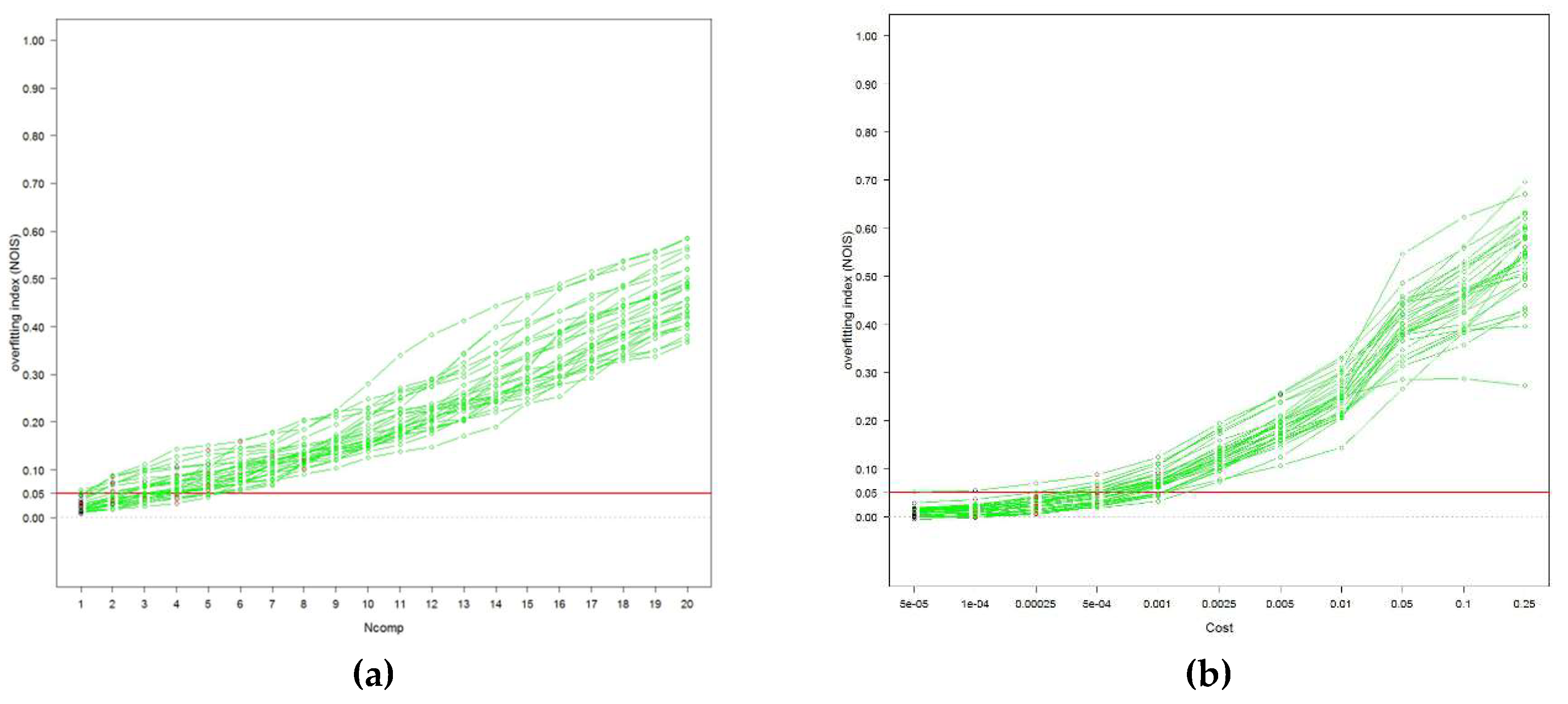The NOIS method selects model complexity considering an a priori level of overfitting tolerated by the user (we used 5%; see Rocha et al., 2017 [25] for details). The complexity selected for models tuned with cross-validation varied according to the landscape. In PLSR up to 20 components could be selected, while in SVM the tuning parameter was chosen among 11 cost values (0.00005 to 0.25). The tuning parameters were fixed across all landscapes when tuning with the NOIS method. Partial Least Square Regression (PLSR) models were fixed with two components, while Support Vector Machine (SVM) models were parameterised with a cost of 0.0001 (Appendix A). Partial Least Square Regression (PLSR) models were fixed with two components, while Support Vector Machine (SVM) models were parameterised with a cost of 0.0001 (Appendix A).

An ordinary least square (simple) regression using a two-band vegetation index was fitted to compare with the machine learning algorithms. The LAI Determining Index (LAIDI), a ratio between two wavelengths (1050 nm and 1250 nm) situated in the NIR spectral domain, was used to predict LAI using linear regression [55]. The wavelengths were selected a priori based on literature, rather than by searching for the band combination that explained most of the variation in the response variable.

The selected model for each regression technique was assessed by the capacity to generalise with similar accuracy when predicting with a new dataset. Therefore, the RMSE calculated from the training set (RMSEtr), the testing set (RMSEtest) and the independent set (RMSEind), were compared to the estimated RMSE of cross-validation (RMSEcv). The testing and independent set were also used to assess model generalisation in a different realisation or spatial dependency (when moving across landscapes vertically or horizontally as in Figure 1).

The Durbin Watson statistic was calculated to quantify autocorrelation in the model residues considering the observations sequentially in space, following the sampling path as depicted in Figure 2, reflecting the spatiotemporal autocorrelation as if the data were collected in the field. The statistic varies between 0 and 4, where values around 2 indicate no autocorrelation, values below 2 indicate positive autocorrelation and values above 2 negative autocorrelations [24].

All the analyses are executed in R version 3.2.2 (The R Foundation for Statistical Computing). The package gstat was used for unconditional simulations, hsdar for simulations of spectra with PROSAIL 5B, and Caret for fitting models from all regression techniques with the same cross-validation approach.

3. Results

3.1. Prediction Accuracy Estimated from the Training Set

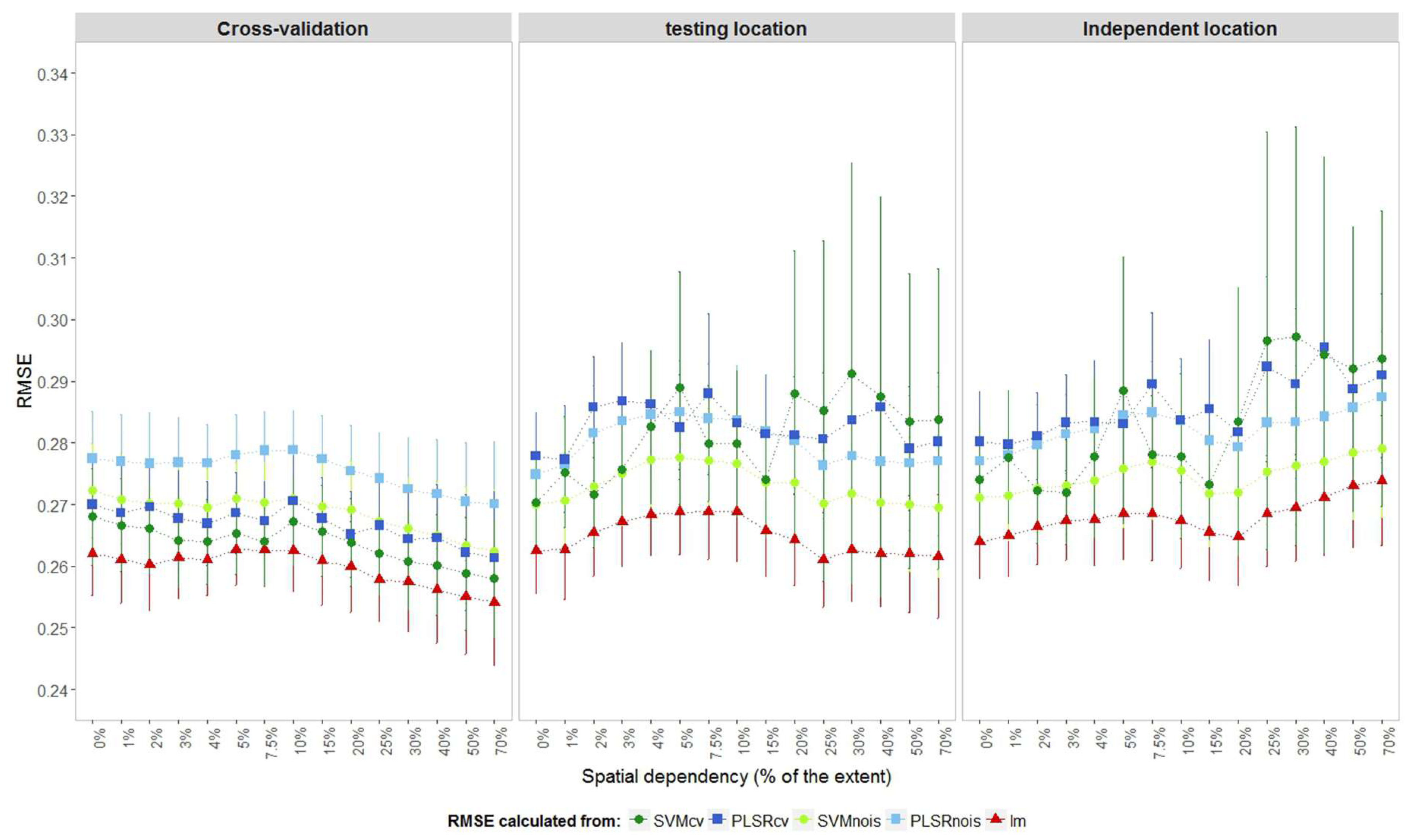
Estimates of RMSE based on the complete dataset used for training the model (RMSEtr), as expected, were smaller than the estimation of the cross-validated partition (RMSEcv; Figure 4). The differences were much larger for the machine learning algorithms tuned with cross-validation (PLSRcv and SVMcv) than for those tuned with the NOIS method. A large gap between the estimated RMSEcv and RMSEtr indicated overfitting, which may be partly caused by learning (i.e., fitting) spatial structures and random noises.

Regardless of the level of spatial dependency, differences between RMSEcv and RMSEtr were relatively small for machine learning models that were tuned with the NOIS method, and practically disappeared for the simple regression (lm). For the PLSRcv and SVMcv models, this difference slightly increased when the spatial dependency increased, because the training error (RMSEtr) decreased faster than the cross-validated error (RMSEcv). This trend is less clear for the less complex models tuned by the NOIS method or the linear models. The RMSEcv from models tuned by cross-validation was smaller, as selection was based on the model complexity that minimises the prediction error.

The LAI values for all artificial landscapes came from the same distribution N~(4,0.5). Thus, across the fifteen levels of spatial dependency no trend should be observed in RMSEcv. Where spatial relations were not captured (fitted) by the model, all variations should come from random differences among the thirty realisations. Model complexities should be similar for all 450 landscapes (15 x 30), as spectra were generated by the same deterministic function from the Radiative Transfer Models (RTMs). However, for instance, the PLSRcv models had levels of complexity ranging from 1 to 12 components. This is a sign that models may be fitting spatial structures and random noises, because these form the only differences within the artificial landscapes. The prediction errors estimated from the training data are more affected by spatial structures and random noise in complex models such as PLSRcv and SVMcv.

3.2. Prediction Accuracy Estimated from Validation Sets

Prediction accuracy can be estimated by observations collected in the same campaign as the training set (so from the same imagery and ground observations) but kept apart for validation instead of cross-validation. Despite being from different sample locations, the observations from the testing set (RMSEtest) contained the same underlying spatial structure as the training set. For more complex models the testing sets presented higher prediction errors than cross-validation estimation did (Figure 4). Simple linear models performed according to the testing set and quite similar to cross-validation, while SVM models tuned with the NOIS method presented the best machine learning performance. For cases where spatial dependency was higher than 15%, RMSEtest values for more complex models presented much higher average errors and wider confidence intervals.

The prediction error can also be estimated by an independent testing set collected in the same landscape, but in a different sampling campaign, represented here by RMSEind. In this case, the predictions presented visibly higher errors than the RMSEtest for spatial dependencies higher than 15% for all models. This occurred because the models fitted spatial relations in the observations that were not supported by any explanatory variable present as these sets had different spatially dependent noises. Overall, prediction errors presented two general types of behaviour across levels of spatial dependency. Firstly, regardless of the type of validation data used, the error increased around levels of spatial dependency that matched the sampling distance (approximately 8% of the extent in our case). Secondly, the error decreased above 15% of spatial dependence, except for complex models validated by the testing set (RMSEtest) or any model validated with the independent set.

3.3. Prediction Accuracy Estimated on a New Realisation

The cause-effect relationship between the reflectance and LAI values is the same for all artificial landscapes, being defined deterministically by the Radiative Transfer Model. Therefore, any empirical model should in theory, produce a similar accuracy when predicting another realisation. This assumption was not confirmed by this study whenever the models were complex or the spatial dependency was strong. The gradual reduction in prediction error (RMSEtest) in landscapes with a spatial dependency higher than 15% was not observed when validated with data from another realisation. This confirms that these models are learning with the spatial distribution of the training set Figure 5.

Two aspects are resulting in a lack of model generalisation. One is caused by the sampling density, resulting in higher prediction errors between 2% and 10% of spatial dependency. This behaviour indicates that sample densities similar to the spatial dependency of the plant trait may produce quite unstable models and reduce the accuracy of the predictions. The other aspect is related to models that were trained in landscapes with strong spatial dependency (more than 15%). The prediction error estimated by cross-validation, in this case, is not observed in a new landscape with the same spatial autocorrelation. In other words, these models were fitted to represent a particular spatial distribution in that dataset, rather than the underlying causal relationship.

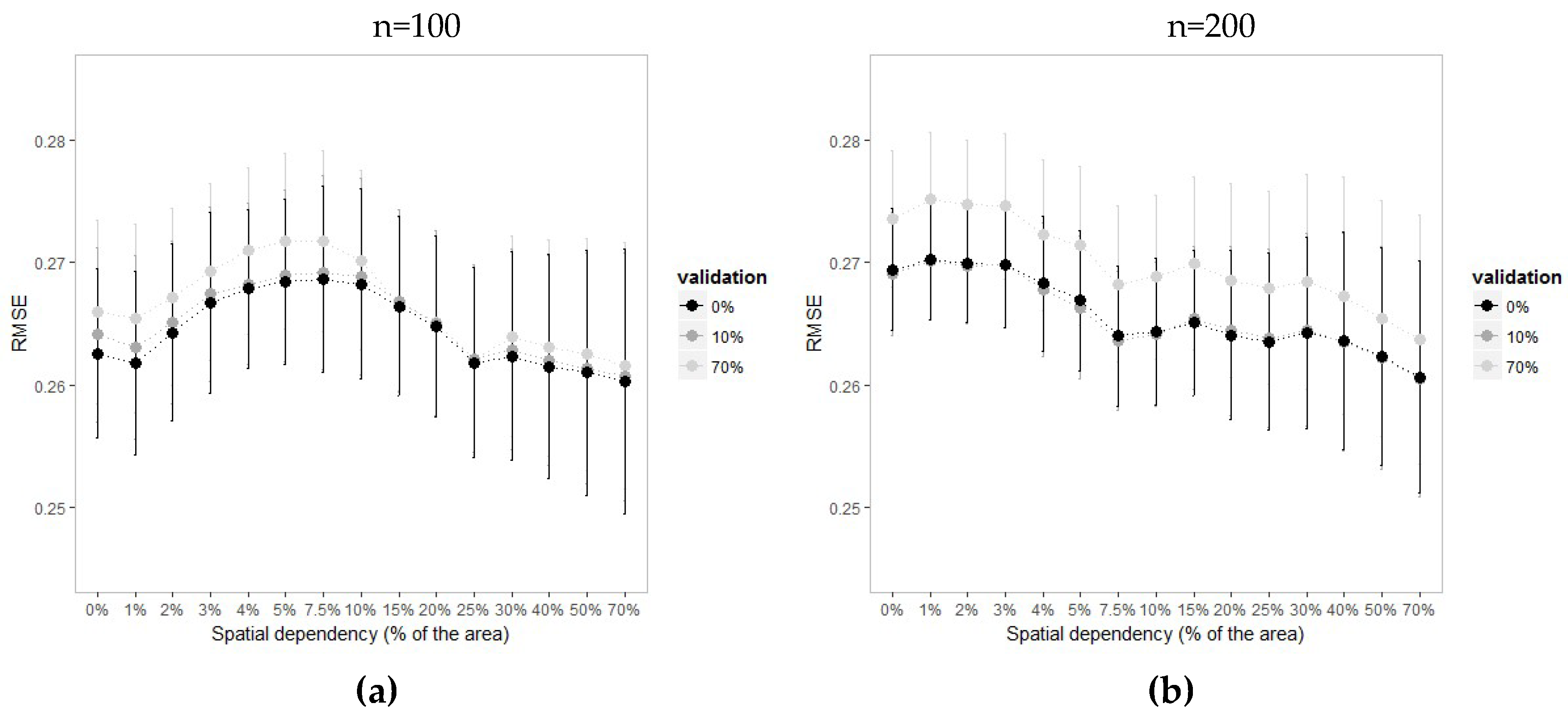
3.4. Prediction Accuracy Estimated on a Different Spatial Dependency

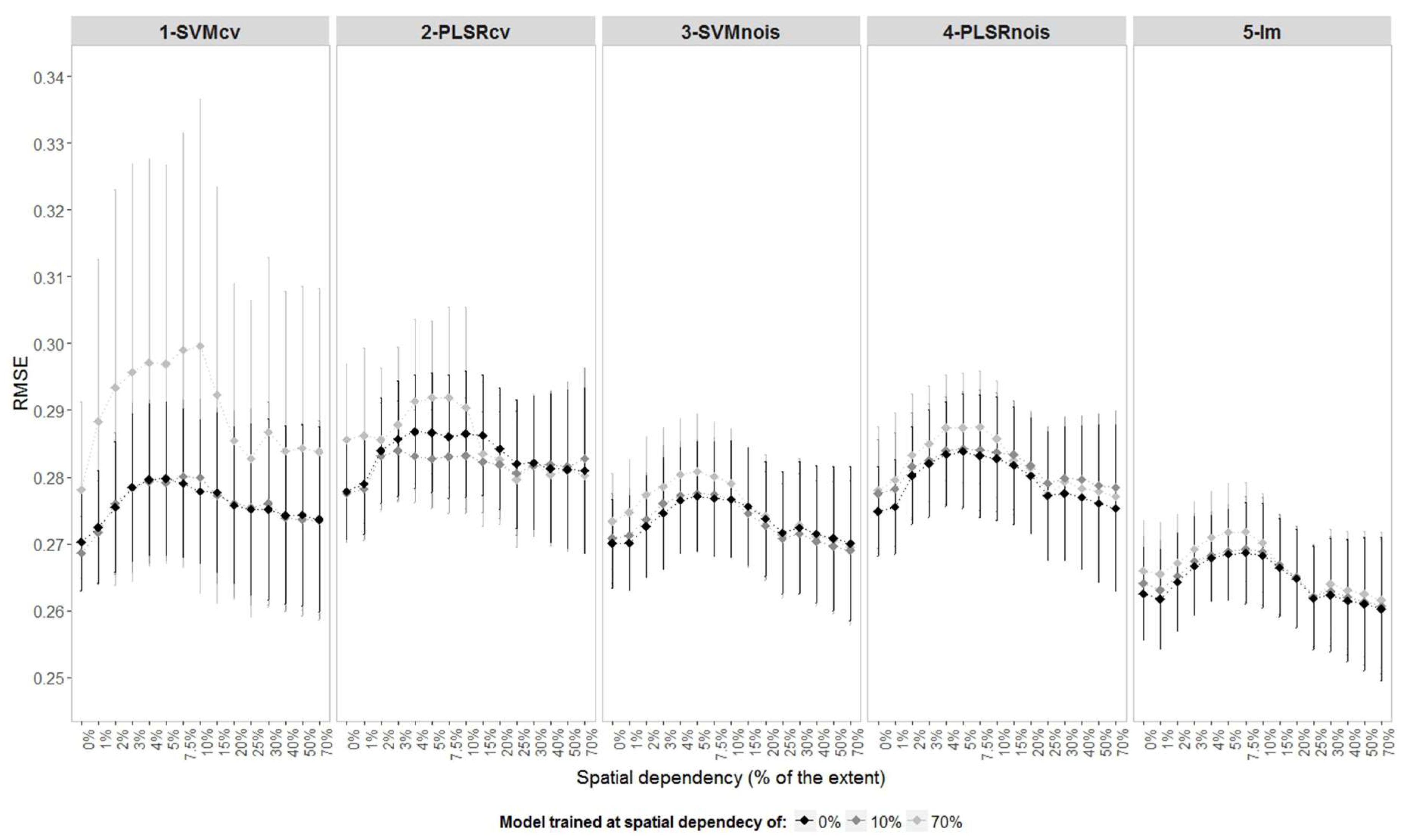
Models trained in landscapes without spatial dependency, in general, produced lower prediction errors when applied to landscapes with other levels of spatial dependency as presented in Figure 6. The models should achieve similar accuracies when used for landscapes having different levels of spatial dependency if they capture only the true relation between reflectance and LAI. However, the higher the spatial dependency used for training a model, the more likely it is that this model will capture undesirable spatial relations from the observations. This is most visible on complex models such as SVMcv, where lower prediction accuracies are observed for models trained on the highest spatial dependency (e.g., 70%, Figure 6).

Regardless of the spatial dependency in the landscape used for training the model, the RMSE increases in the landscapes with levels of spatial dependency between 2% and 10%. In this interval, the PLSRcv models present lower prediction error when trained under 10% of spatial dependency. If the sample size is reduced, the highest values of RMSE shift to landscapes with stronger spatially dependency, while the effect moves in the opposite direction when the sampling density is increased (Appendix B).

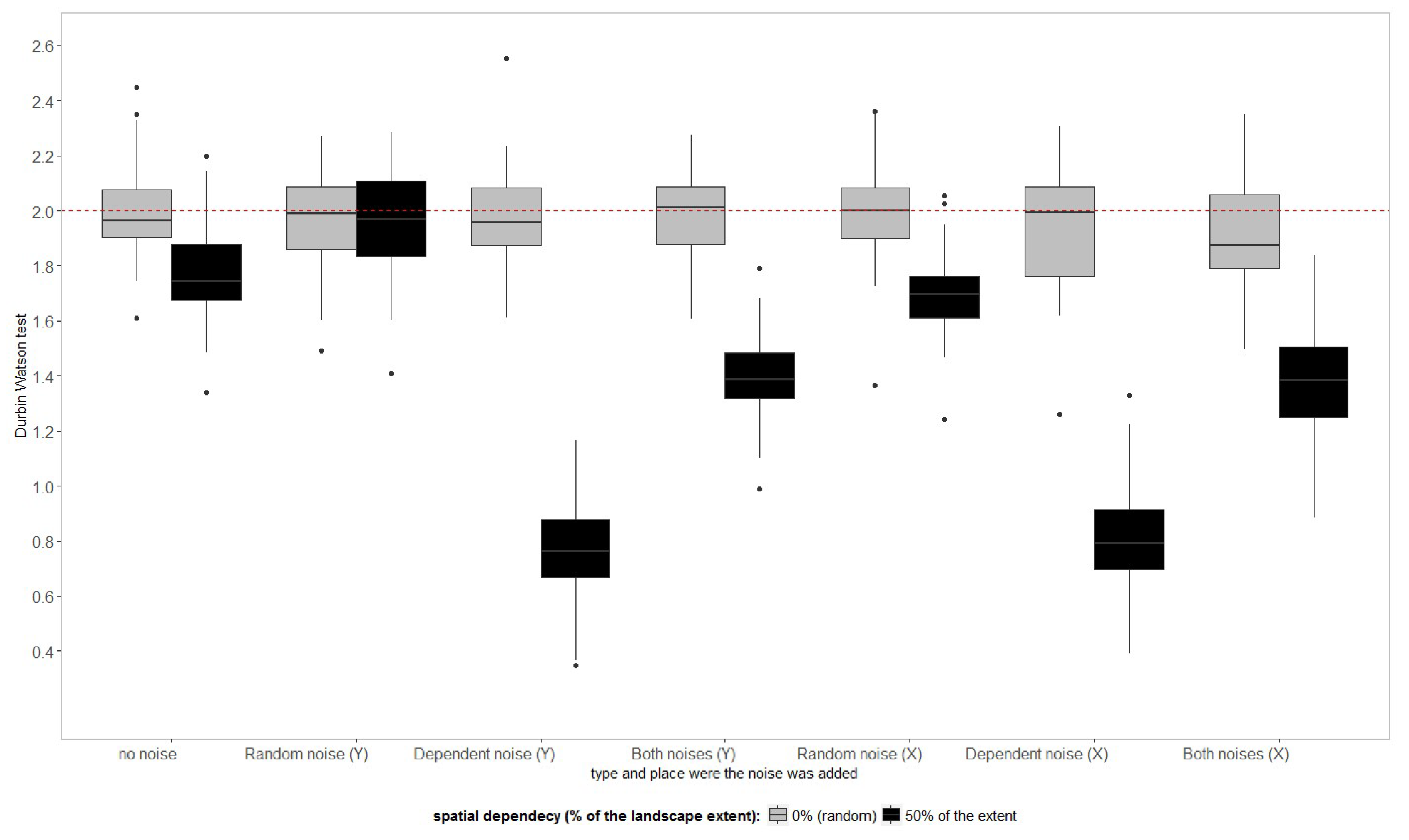
3.5. The Effect of Spatial Dependency on Model Assumptions

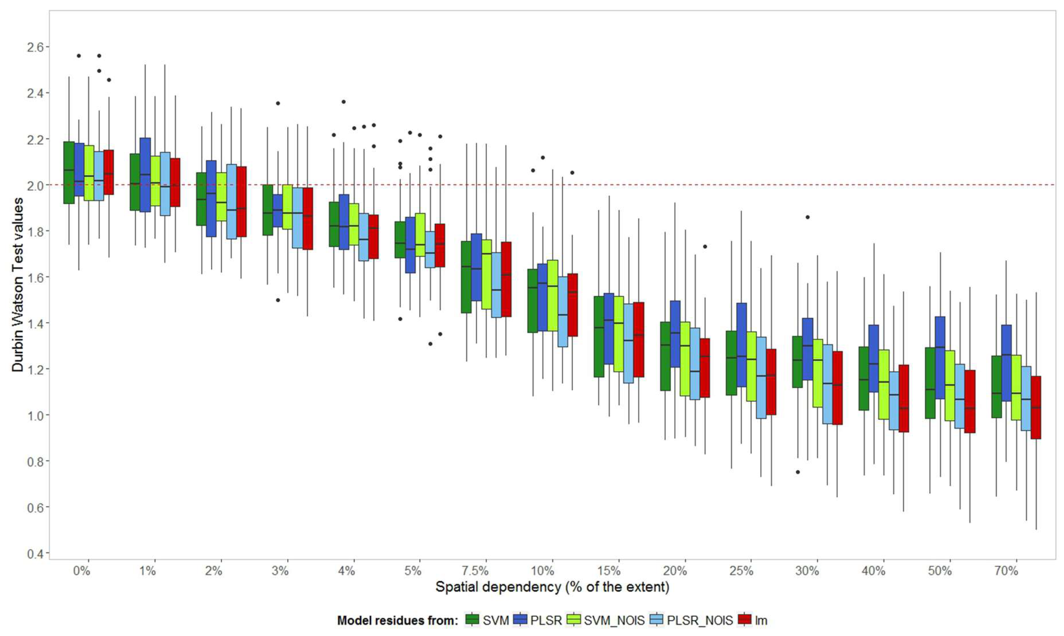
Model residues should be normally distributed with mean zero, but should also be randomly distributed in space and time. Non-spatial models using spatially dependent observations might not fulfil these assumptions. The Durbin Watson (DW) statistics (Figure 7) show the presence of significant autocorrelation in the residues for models that are trained in landscapes with the spatial dependency of 5% and above, departing clearly from the baseline represented by the value 2.

The autocorrelation in the model residues is less strong for the more complex models (PLSR_CV and SVM_CV) compared to the more simple models (SVM_NOIS and LM). Autocorrelation may not be detected in the final model residues in machine learning algorithms when sufficient latent variables are created to explain all the residues. Figure 7 shows some outliers for machine learning trained with data that had 20% to 40% of spatial dependency supporting this claim. If most of the spatial structures of the response variable (LAI) are explained by the spectra, the model residues might also not present significant spatial autocorrelation (Appendix C). This would occur if spatially dependent noise was not added in this study before modelling. However, in a real case scenario, it is unlikely that remote sensing data of a canopy will only explain the spatial dependency of the target plant trait.

4. Discussion

4.1. Spatial Dependency and Prediction Accuracy

Plant traits are likely to exhibit spatial dependency in continuous landscapes regardless the extent or spatial resolution of the measurements [7,9]. Therefore, when the objective is to compare plant trait predictions from similar landscapes or monitoring the same landscape over time, a model needs to be carefully fitted and tested. An important consideration should be to avoid modelling spatial relations in the observations when these are not causally linked to the plant trait under investigation. Otherwise, these models should be considered to be “single-use” models that have little capacity to predict when new spectral data are available.

This study shows that training complex models when using high dimensional data, such as hyperspectral measurements, presents a considerable risk of underestimating prediction error. This occurs because models may overfit by capturing random noise from a large number of wavelengths, often supported by insufficient observations. The risk grows when model complexity increases and in the event of spatial dependency in the plant traits. Here we showed that machine learning models tuned by cross-validation seemed to learn from spatial structures and fit spurious correlations between random noise and LAI, suggesting an increase in performance.

A linear regression using a predefined two bands ratio index reduces this risk of overfitting by decreasing the effect of multicollinearity and lack of degree of freedom caused by a large number of predictors available. However, if a linear regression is selected through a stepwise algorithm with all spectral bands, or using a vegetation index that searches the combinations of two or more bands provides the best correlation with the plant trait (i.e., supervised feature selection), the risk of overfitting is also expected to be high, regardless of how simple the final model is [26,56].

Optimistic estimation of RMSE can also be the result of using cross-validation procedures when testing data is set apart from the same sampling effort as the training data. This is especially noticeable when significant spatial structures are present in the data (compare RMSEcv with RMSEind in Figure 4). With a large number of predictors available, the cross-validation tuning process seemed to select models that partially fit variations in the data rather than in the underlying phenomenon.

Less complex models tuned by the NOIS method or linear models present more reliable estimations of the prediction errors, but these also tend to be underestimated when the spatial dependency is not well covered by the sampling density. In our simulations, this was the case when spatial dependency was less than the average distance between sampling locations (i.e., landscapes with a spatial dependency of less than 10%). The spatial dependency of plant traits should be used to define the optimal distance between samples. However, in most cases, this information is only known after the data is collected [57]. If remote sensing images are available before the sampling campaign, these could be used as reference to estimate the expected spatial dependency from wavelengths known to be correlated with the desirable plant trait.

The primary goal of model fitting is to learn the empirical relationship between reflectance and plant traits for a determinate landscape. In this study, this implied that the models should approximate the function used by the Radiative Transfer Models to simulated reflectance from LAI values. When the model learns with spatial structures and random noises in the data, instead of the underlying relationships, it produces misleading inferences and results in underestimating prediction errors.

4.2. Beyond the Scope of These Simulations

A number of simplifications and restrictive assumptions were used to simulate spectral data that only vary spatially in relation to LAI values. For instance, all plant traits used as parameters by the RTM to simulate spectra had the same level of spatial dependency as LAI within each realisation. The spatial structure introduced by noise in both LAI and spectral data presented the same level of spatial dependency. These assumptions might be unrealistic as, despite the potential correlation among plant traits, it is more likely that spatial dependency occurs at different levels.

Reflectance values may also present different spatial structures based on the wavelength regions and their sensitivity to the different plant traits. In addition, other spatial structures related to the landscape, such as soil moisture and its effect on background reflectance, will be captured in spectral datasets. Temporal structures can also be captured as optical sensors, and ground-truth measurements are hardly ever collected simultaneously and therefore are not entirely free of systematic errors. All these factors and their combinations can exponentially increase the risk of overfitting. In real-life environments, which are not as controlled as in the presented study, the underestimation of the prediction error is probably even higher for complex models through learning from the spatiotemporal structure in the training data.

Although machine leaning regressions are known for not requiring assumptions such as independent and identical distributed observations nor model residues, their effect on model prediction may be even stronger than with ordinary least squared regressions. The relaxation of assumptions such as the absence of multicollinearity and spatial autocorrelation, or principles such as model parsimony, does not mean that their effect on model predictions is negligible. Due to the high dimensionality of hyperspectral data, machine learning is often used for modelling plant traits based only on spectral data. Classical assessment comparing spatial and non-spatial models are based on how they manage to decrease or eliminate spatial autocorrelation in the residuals [43]. Machine learning algorithms cannot be compared in this way, as they often use the residuals to improve the model.

4.3. Spatiotemporal Structures in Remote Sensing

Water availability, species dominance, slopes, nutrient concentrations in the soil and many more factors can drive the spatial dependency of plant traits in nature. If measurements from continuous vegetation (landscapes) do not contain spatial structures, they are not an accurate description of nature, limiting the understanding of the target surface [58]. As it is known that nature is stochastic and does not repeat a process under the same conditions, temporal structures can also affect prediction accuracy.

Spectral measurements may vary over the course of a day by capturing changes in the relation between sun altitude and viewing angles at the same location. Variations can also occur on a medium to long-term time scale, related to weather conditions or seasonal plant cycles. Organising a field campaign using a limited period of the day to control for solar azimuth may require many days to complete the data collection. This may decrease the variation in illumination geometry but will increase differences in plant phenology or maximum sun zenith. In contrast, an intensive and short campaign may have to use many hours per day, increasing variability in illumination conditions and the autocorrelation between consecutive measurements. This trade-off in sources of error will depend on the plant trait of interest, sample design and instruments used.

Both, plant traits and reflectance values, for instance, can be captured by optical sensors in the field (e.g., LAI using LAI2200 and spectral data with an ASD spectrometer). In this case, the risk of undesirable spatiotemporal structures in the data is higher than when ground-truth is measured in the lab, and spectral data come from the same scene of a satellite image. In satellite or airborne data, the difference in geometrical distortion (changes in the field of view) within the scene or in time between two scenes (in the same swath or not) may also provoke spatiotemporal patterns. Other data structures rather than spatiotemporal, such as phylogenetic or genetic relations may also lead to dependency in the multi-species analysis [9]. In a lab experiment illumination and view angles can be well controlled, however, combinations such as repeated samples from a set of different plant species, growth stages or levels of stress may create a sequence in the data that can lead to similar effects as spatiotemporal structure if modelled together [9].

Modelled plant traits from a landscape using hyperspectral data likely present at least three sources of spatial autocorrelation in the data: (1) the spatial pattern of the landscape determined by the underlying process that drives the plant trait, in this study represented by the different realisations of LAI values correlated in space; (2) the spatial autocorrelation in the ground measurements determined by the sampling footprint used for training, illustrated here by the path of a sequential sample; and (3) the autocorrelation related to noise from the optical sensor and ground measurements, as data is captured neither simultaneously, nor independently in space (included in this study as spatial dependent noise). The first source is of natural origin (inherent) and should be modelled with an approach that takes the spatial structure explicitly into account whenever it is not fully explained by the reflectance values (Appendix C). Although, to model the spatial structure of the plant trait properly, the sample design and density (second source) have to be spatially representative [59]. The third source of autocorrelation can mislead the second and might be considered a sort of bias or distortion that should be corrected before modelling. For instance, whether or not a spatial structure in remote sensing data caused by soil background should be treated as a systematic error or modelled as part of the underlying process, will depend on whether the plant trait under consideration is also related to process, or only affects the reflectance values.

Appropriate sampling design and a well-controlled measurement campaign can significantly reduce random and systematic noise in the measurements, but will never eliminate all noise, so model validation with new (unseen) observations that do not stem from the same sampling effort is essential to achieving model generalisation. Lastly, in this study, we showed that the choice of sample size could affect generalisation in different ways. Models trained with a small sample size may increase overfitting as a small sample size reduces the number of observations to support a large number of predictors. Larger samples reduce the distance between the points, changing the sensitivity to the spatial dependency and increasing model complexity (Appendix B). Remote sensing data provide an opportunity to study the spatial structure in a landscape before planning fieldwork to collect ground-truth measurements. This opportunity should be grasped more often to determine sample design and point density in order to avoid or properly model spatiotemporal structures.

5. Conclusions

Machine learning regressions using hyperspectral data to predict plant traits are sensitive to overfitting if careful model tuning is not conducted. In the presence of strong spatial autocorrelation, the risk of overfitting increases considerably, and there is no obvious solution to correct this for machine learnings. The result is that models have lower actual prediction accuracies than those estimated by cross-validation. Spatial structures should not mistakenly be interpreted as causal relationships between spectra and the trait of interest. When spatial structures are inherent to the underlying process that drives the trait but are not completely explained by the spectra, they could be modelled with a method that accounts explicitly for the spatial structure. As illustrated in this study, the effect of the spatial dependency can be easily detected in model residues by conventional autocorrelation tests using a sequence of sampling plots. Robust model validation and tuning approaches to restricting complexity in machine learning algorithms, such as the NOIS method, can help to reduce the risk of producing “single use” models that cannot be applied in any other area or at any other time than for which they were trained.