Fractal-Based Local Range Slope Estimation from Single SAR Image with Applications to SAR Despeckling and Topographic Mapping


Department of Information Technology and Electrical Engineering, University of Naples “Federico II”, 80125 Naples, Italy
*
Author to whom correspondence should be addressed.
Remote Sens. 2018, 10(8), 1294; https://doi.org/10.3390/rs10081294
Submission received: 26 June 2018
/
Revised: 17 July 2018
/
Accepted: 10 August 2018
/
Published: 15 August 2018
Abstract
:In this paper, we propose a range slope estimation procedure from single synthetic aperture radar (SAR) images with both methodological and applicative innovations. The retrieval algorithm is based on an analytical linearized direct model, which relates the SAR intensity data to the range local slopes and encompasses both a surface model and an electromagnetic scattering model. Scene topography is described via fractal geometry, whereas the Small Perturbation Method is adopted to represent the scattering behavior of the surface. The range slope map is then used to estimate the surface topography and the local incidence angle map. For topographic mapping applications, also referred to as shape from shading, a regularization procedure is derived to recover the azimuth local slope and reduce distortions. Then we present a new intriguing application of the inversion procedure in the field of SAR despeckling. Proposed techniques and high-level products are tested in a wide series of experiments, where the algorithms are applied to both simulated (canonical) and actual SAR images. It is proved that the proposed range slope retrieval technique can (1) provide an estimate of the surface shape, with overall better performance w.r.t. typical models used in this field and (2) be useful in advanced despeckling techniques.

1. Introduction
In recent years, theoretical analyses and experimental proofs highlighted the possibility of extracting more and more information from synthetic aperture radar (SAR) images, obtaining value-added products that help in making SAR systems more accessible and understandable to non-expert users [1]. In addition, the study of extraterrestrial bodies and the search for extrasolar planets is always of great interest, as demonstrated by recent missions such as the Cassini-Huygens mission to Saturn and the ESA planned JUICE (Jupiter Icy moons Explorer) mission [2]. In this context, the estimation of topographic parameters (e.g., local slopes) from (single) SAR images represents an important topic not only per se, but also because from the topographic content of the sensed surface geologists and astrophysicists can derive other important indications regarding both planet activity and future missions’ design [3,4,5,6].
Up to now, many techniques aimed at retrieving topographic content from remotely sensed data have been developed, namely stereoscopy [7,8], interferometry [9], radarclinometry—or shape from shading (SfS)—[10,11,12,13,14,15] and polarimetry [16,17], each with its own advantages and drawbacks. Unlike the other techniques, which require (a minimum of) two complex SAR images, possibly acquired at the same time, SfS has the main feature and advantage of requiring just one intensity image. Other existing techniques, as radar and laser altimetry, require no images at all [18,19]. However, they provide one-dimensional (1-D) height profiles rather than two-dimensional (2-D) maps, thus requiring a huge number of passes and some kind of interpolation methods in order to link the different profiles and provide an estimation of the underlying topography. The multiple-pass acquisition system and the relative low accuracy make these techniques not suitable for digital elevation model (DEM) retrieval. Nonetheless, altimetry data are useful in SfS and can be exploited as a priori information.
Since the seminal work by J. van Diggelen [20], and the subsequent works of Wildey [11,21], Horn [12,13], and Frankot and Chellappa [22], SfS techniques have now reached a high level of accuracy, reliability, and robustness within the area of optical imaging, where very accurate SfS algorithms have been developed [13]. Conversely, little has been obtained from SfS techniques applied to SAR images. The main reason for this lack of results stands in the ill-posedness of the problem due to the fact that two variables, namely the local slopes on orthogonal directions, have to be retrieved from a single intensity image. Roughly speaking, SfS techniques have to deal with the retrieval of two unknowns from a single equation. In addition, a large number of physical parameters affect SAR image formation; e.g., the dielectric properties and the small-scale roughness of the observed surface. Therefore, the SfS problem is, in general, under-constrained and simplifying assumptions on the dielectric and roughness behavior of the surface are enforced in the existing literature. In particular, the dependence of image intensity on large-scale slope is mostly modeled using the same Lambertian or Lambertian-like models used for optical images, while the dependence on the physical parameters of the surface (electromagnetic parameters and small-scale roughness) are rarely modeled at all. Therefore, the widespread assumption of uniform dielectric and roughness properties for the surface is not based on a physical reasoning, but simply on the rough guess that the topography provides the main contribution to SAR image formation, at least in scenes where it is significantly present. Actually, without further insights on the nature of the involved dependencies, we are left in the presence of a conceptually unsolvable problem. Hence, the research on this topic reached a point in which the only possibility to obtain new results lies in the introduction of sound direct models for microwave scattering that explicitly depend on the physical parameters of the problem. In this case, even in situations where most of these parameters are unknown, the model can help in gaining a better understanding on some relevant properties of the scene.
In this paper, we propose a novel approach to topographic content retrieval based on fractals, for modeling both the roughness of the observed natural surface and the electromagnetic scattering. In contrast with other existing techniques ([10,16,17,23,24,25,26,27])—in which very simple models (or their generalization) appropriate to describe scattering in the optical region are extended in some way in the microwave region or some heuristic approaches are introduced in order to correct them—we propose a complete model-based approach. In particular, starting from a fractal surface model appropriate for natural landscapes, we introduce a direct model able to properly describe the complex electromagnetic phenomena characterizing the scattering from natural surfaces in the microwave region, where SAR systems usually operate. To this end, the problem is decomposed in two steps: first, the surface roughness is described via fractal geometry as a 2-D fractional Brownian motion (fBm) and the Small Perturbation Method (SPM) suitable for such a surface model is adopted as a scattering model to derive the normalized radar cross-section (NRCS). Then, the NRCS is linked to the SAR intensity map through an imaging model. In order to cope with the ill-posedness of the problem and simplify the inversion procedure, we derive a linearized model, which is valid in a small-slope regime and enables us to estimate the range slope. Moreover, as already shown in [28], the first order expansion of the model is shown to be independent on the azimuth slope. An absolute calibration procedure is provided as well.
In the very frequent case in which no a priori knowledge about the surface properties is available, the involved physical parameters can be assumed to be constant over the scene, on the basis of the observation that the main contribution is the topographic one. In actual cases, this hypothesis is unreal and very restrictive; however, in presence of little variation of the characteristics of the surface, the algorithm can still provide acceptable results. Anyway, the model itself does not dictate the requirement of homogeneity of surface characteristics; in fact, whenever some kind of a priori knowledge is available it can be easily injected within the model. For instance, the model can readily include information on the fractal parameters of the scene retrieved from the same SAR amplitude image using the technique proposed in [28], or any kind of information on soil characteristics estimated from multispectral sensors.
The range slope map is then exploited in both standard and innovative applications, namely topographic mapping; i.e., DEM estimation, and SAR despeckling based on a priori scattering information. Concerning the former application, while most state-of-the art techniques are based on the use of polarimetric data (and thus multiple acquisitions) to account for azimuth slopes [16] or simply neglect azimuth slopes [23], we propose an algorithm that employs a regularization procedure to recover the azimuth slopes. In [14,15] the azimuthal component of the slope is estimated through a regularization procedure based on an iterative optimization process. In the present paper we show that, by strengthening the direct model through the introduction of proper direct models for surface and scattering mechanisms, it is possible to estimate the underlying topography also with a very simple and low computational complexity inversion technique. With regard to the other parameters needed by the proposed inversion algorithm, we use reference values or we assume their a priori knowledge, as detailed in the body of the paper. Even if on the Earth’s surface more convenient and accurate methods can be enforced for DEM estimation, this application still holds a prominent role in extraterrestrial bodies’ exploration, where even a coarser DEM can be useful for geophysical interpretation [3,4,5,6,29].
Besides topographic mapping, it is here demonstrated that range slopes can be conveniently applied to SAR despeckling. To this aim, local slopes are exploited for the estimation of the local incidence angle, which in turn is exploited in the SB-PPB filter, a recent despeckling algorithm based on scattering [30,31,32]. Such algorithms introduce physical insights in conventional despeckling by injecting a priori scattering information about the illuminated surface in pre-existing filters. The required a priori information mainly concerns the local incidence angle, since this is the most relevant factor influencing SAR image formation [30]. In [30,31,32], a DEM gathered from independent sources (e.g., SAR interferometry, stereoscopy, lidar) is exploited to retrieve such a priori knowledge. In this paper, we demonstrate that the topographic content required in scattering-based despeckling can be conveniently estimated directly from the SAR image, thus avoiding the requirement of extra information and data.
The paper is organized as follows. Section 2.1 is devoted to derive an analytical relationship between SAR image intensity and the parameters of interest; i.e., the local slopes of the illuminated surface. The inversion of the direct model is discussed in Section 2.2, and related high-level products and applications (topographic mapping, despeckling) are defined in Section 2.3. Experimental results are presented and discussed in Section 3. First, we apply our framework on simulated data: in this case, synthesized DEMs are generated and used as ground-truth, while corresponding SAR images are simulated with a SAR signal simulator and used as input for SfS. The results presented in Section 3.1 are useful to investigate the validity of model hypotheses. For the other canonical cases, results concerning both DEM estimation and despeckling are reported. A quantitative assessment of the applications is presented. Finally, Section 4 concludes the paper with some remarks and recommendations for future work.
2. Materials and Methods
2.1. Direct Model
In this section, the rationale for expressing the link between SAR image intensity and the local slopes of the surface is presented. The proposed direct model is divided in three parts: first, the natural surface under study is properly modeled using fractal geometry; in particular, a fBm is used. Actually, to cope with the non-differentiability of the fBm process and the limited range of fractalness of natural surfaces, a smoothed version of the original fBm process must be introduced (physical fBm).
The second step consists in adopting a scattering model; i.e., a method for the evaluation of the field scattered from the previously modeled natural surface. In this step, a relationship between the backscattering coefficient and the geometrical (in particular, local slopes) and electromagnetic parameters of the surface is derived.
The last step consists in the determination of a model for the SAR image, linking the measured intensity map to the backscattering coefficient and to the local slopes of the surface. This complete model-based (surface, scattering and imaging models) approach is a key feature to properly devise an inversion procedure allowing to somehow circumvent the ill-posedness of the problem and physically justify information extraction from even a single SAR image. The proposed model is in sharp contrast with other existing techniques in which only the imaging models, mostly derived from optics, are used [10,16] and only sparse considerations on electromagnetic scattering are made [33].
2.1.1. Surface Model
Several models describing natural surfaces’ roughness have been presented. Furthermore, there is increasing experimental evidence that the fractal geometry represents the most appropriate mathematical environment to describe the shape of natural surfaces [34,35,36]; in addition, extensive literature deals with fractal scaling of natural surface roughness [37,38,39]; furthermore, fractal approaches provide a description of the surface with a minimum number of independent parameters [40]. One of the reasons for this success is the ability of fractal models to properly account for the statistical scale-invariance properties (in particular, self-affinity) of natural surfaces. Analytic models reported here are able to handle a variety of natural surfaces: bare and moderately vegetated soils, as well as ocean surfaces. In particular, we adopt here a (topological) 2-D fBm stochastic process z(x,y) defined as follows [40]:
where Pr{} stands for “probability”, is the considered height increment, z(x,y) is the surface elevation and
is the distance between the two considered points of coordinates (x,y) and (x′,y′) and
- H: Hurst coefficient (0 < H < 1) related to the fractal dimension D = 3 − H;
- T: topothesy [m], i.e., the distance over which chords joining points on the surface have a surface-slope mean-square deviation equal to unity.
Fractal geometry exhibits self-affinity properties at any scale and does not allow the derivative operation at any point. Therefore, mathematical fractals cannot be directly applied in scattering problems. However, natural surfaces are observed, sensed, measured, and represented via instruments that are, for their intrinsic nature, band-limited. In other words, no actual natural surface holds property (1) at every scale, and some properties of fBm mathematical surfaces may be relaxed [40].
2.1.2. Scattering Model
The second step is the selection of a scattering model. Here we consider the SPM since it provides analytical closed-form equations, showing a range of validity adequate to SAR applications. Indeed, this method provides a very simple relation between fractals parameters and the backscattered field.
Considering a monostatic configuration and assuming that the surface can be described as a physical fBm, the backscattering coefficient under SPM can be expressed as [41]
wherein m and n stand for the transmitted and received polarization (horizontal or vertical), respectively, k is the electromagnetic wavenumber of the incident field. S0 characterizing the spectral behavior of the physical fBm surface, is expressed in [m(−2−2H)] and related to T and H [40]; , accounting for the incident and reflected fields polarization, is a function of both the complex dielectric constant εr of the surface and the local incidence angle θ [40]. Note that, with this model, we are able to deal only with the co-polarized case; in this case, it is possible to consider the term ||2 constant with θ in the angular interval of interest.
Figure 1 shows a graphical comparison between the proposed fractal scattering model and the Lambertian one. The strong non-linearity of the proposed fractal model can be appreciated; unlike Lambertian law, it is also not upper-bounded, thus forecasting an infinite energy scattered in normal incidence conditions. This behavior, clearly in contrast with the physics of scattering phenomena, is due to the approximation used to obtain the SPM solution, which is applicable only in a small slope regime. However, both the scattering models go to zero under grazing incidence conditions.
2.1.3. Imaging Model
In this section, we derive a relationship between the SAR intensity image and the slopes of the observed surface in order to apply the SfS algorithm. The following model for the intensity SAR image is used [42]:
where I is the SAR intensity image and G is a calibration constant.
Substituting (3) in (4), we obtain the desired relationship between the intensity map I and the range and azimuth slopes
In order to express the intensity image in terms of the local surface slopes, let us introduce the partial derivatives of the surface z(x,y) along ground-range (p) and azimuth (q) directions
Hence, it is necessary to link the local incidence angle θ to the local slopes p and q; it can be easily noted that θ is the angle between the propagation unit vector and the surface normal unit vector, so that it can be expressed as:
Expressing also in terms of local slopes, the backscattering coefficient can be rewritten in the following form:
Finally, the SAR image intensity can be linked to the local slopes as follows:
Incidentally we note that the direct model presented in (9) clarifies the ill-posedness of the SfS problem (two unknowns, p and q, to be retrieved from (9)) and identifies the numerous parameters (linked to both the sensor and the surface) on which SAR imagery depends. The use of analytical models for both scattering phenomena and surface shape makes us more aware on how these parameters affect SAR image formation, emphasizing the ill-posedness of the SAR SfS problem, and more in general, of any inversion procedure from a single SAR image. At the same time, a proper modeling of the problem gives the chance of circumventing the ill-posedness, making possible the estimation of the parameters of interest. Indeed, the sensitivity analysis shown in [30] demonstrates the major contribution to the SAR image formation due to macroscopic roughness (i.e., to the local incidence angle), whereas the other parameters provide a minor contribution.
2.2. Model Inversion
The retrieval of information from remote sensing data of the atmosphere, ocean, and land is basically an inverse problem. It is frequently an ill-posed problem, since many geophysical parameters concur to determine the quantities detected by the sensor (the observations), where different combinations of these parameters can give rise to similar observed quantities. Moreover, errors are always present in the measurements as well as in the knowledge of the causal model (the so-called direct or forward model) that relates the parameters to the observations.
Due to the usual lack of a priori knowledge of the characteristics of the observed surface, the proposed inversion method assumes spatial invariance of the dielectric properties of the sensed scene, more precisely the spatial homogeneity of the dielectric constant of the imaged topography. This hypothesis is embedded in the stricter assumption of invariance of the Fresnel reflection coefficient βmn, which is made for the sake of simplicity in order to obtain a less involved inversion technique. Spatial changes of dielectric characteristics (i.e., in general of the complex relative permittivity εr) in SAR images can be mainly related to changes in the material that covers surface (for example water, snow, soil, rock, ice, oil, etc.) or to changes in soil moisture content (dry or wet soil).
As described previously in the paper, natural landscapes exhibit a fractal behavior varying both in space and in scale. This means that both H and T may be modeled as a function of spatial and scale variables. However, in order to deal with a simplified forward model and to exploit existing algorithms for fractal parameter estimation, e.g., [28,43], the proposed model assumes a scale-invariance of both the Hurst coefficient and topothesy; i.e., the multifractal behavior of natural surfaces is neglected.
While these problems are relevant to every SAR image and inversion technique, SfS has to deal with another important issue: being available only one intensity image, the inversion procedure has to retrieve two unknowns—p and q—from a single intensity measurement. From these considerations we can understand the successful choice of fractal geometry: it is required the knowledge of only two independent parameters, that, in turn, are independent from radar viewing geometry and sensor parameters (frequency, resolution, look angle) [43].
In this section, the proposed inversion technique is analytically derived, and its limits are analyzed. In order to simplify the inversion procedure, and then retrieve the range slope map, we assume a small-slope regime for the surface. Thanks to this hypothesis, a first-order approximation of the intensity map I, through a McLaurin series expansion with respect to p and q can be considered:
where o(∙) stands for small-o notation.
It can be proved that [28], so that we obtain a linear function of the partial derivative p only. The intensity function I is, in the first-order approximation, linearly linked only to the range slope of the surface. As a consequence,
The coefficients of the McLaurin series expansion, a0 and a1, depend on the specific adopted direct scattering model. In particular, these coefficients are a function of the sensor look angle, which is hence an important parameter for the determination of the validity limits of the proposed linear model. Finally, we note that the obtained result highlights a key property of SAR—and, more in general, of side-looking radars-imaging behavior, showing a clear mathematical definition of a preferential imaging direction due to their particular acquisition geometry.
It can be shown that for the expression in (11)
Linearization greatly simplifies the inversion procedure, allowing the estimation of the local range slopes in a very straightforward and fast way.
In order to get a valid slope map, it is necessary to devise a procedure aimed at evaluating the calibration constant G that appears in (11). In this work, we propose a very simple way to estimate G from the data; from (11) we have
Since a0 is known, (13) implies that it is possible to estimate the value of G simply by measuring from data the intensity of a flat homogeneous region. Speckle and roughness could affect the estimation, so it is necessary to consider a sufficiently wide flat area or, alternatively, a despeckling algorithm should be applied to the noisy image to obtain a good estimate of G. Obviously, the main disadvantage of this procedure is that it requires a basic knowledge of the sensed scene in order to identify a flat region in the SAR image.
If such a priori knowledge is not available, assuming the validity of the linear model in (11), the calibration constant G can be calculated as follows
where μI is the estimated mean value of the intensity map I. This procedure, based on the assumption that, according to the fractal model assumed, the global mean slope observed in a SAR image of a natural surface is zero, greatly simplifies the inversion technique, since the knowledge of a flat region present in the intensity image is no longer necessary. Furthermore, this hypothesis drastically reduces the amount of a priori knowledge required: if only the shape of the surface is of interest, no knowledge is required, apart from sensor parameters. Additionally, H can be estimated from data using a linear regression of the range cut of the image power spectra (for more details see [28]). It is noteworthy that the retrieval algorithm proposed in [28] estimates a large-scale Hurst coefficient (i.e., the macroscopic roughness), while, at least in principle, we need a microscopic characterization of the resolution cell. However, thanks to the scale-invariance hypothesis, H is assumed to be constant at any observation scale. In addition, it can be easily shown that both T and εr do not affect topography estimation if (14) is used, since they simplify in (13). Thus, using (14):
This means that, if G is evaluated according to (14), the estimated range slope depends only on the ratio between the coefficients a0 and a1. According to (12), in this ratio both |βmn|2 (in which εr is present) and S0 (in which T is present) cancel out. From now on, in order to simplify the notation, we perform a formal substitution, incorporating the calibration constant within the coefficients a0 and a1, so that, hereafter, the linear imaging model becomes
Error Source Evaluation
In this section, some considerations about range slope estimation are emphasized and the main error sources are analyzed and discussed. Starting from (11), it is clear that errors on range slope estimation are caused by errors on the linear model coefficients and the calibration constant. Errors on coefficients are linked to model error; i.e., the linear approximation of the intensity image and to parameter errors; i.e., errors on geometric and electromagnetic parameters of both surface and sensor; errors on G are due to model error concerning G evaluation (see Equation (14)) and, as we will also show, to errors committed on a0 and a1.
In the following, we note by an estimator of x. Considering an additive error ΔG on G estimation we obtain:
Equation (17) means that an error ΔG cause a rescaling and a translation of the estimated range slope and, as a consequence, the estimated topography suffers from a rescaling and a tilt depending on the relative error and the coefficients ratio.
The same effects are caused by an error on model coefficients:
where Δa0 and Δa1 the error on coefficients.
In a more realistic scenario, errors on both calibration constant and coefficients are present; in this case, more severe distortion effects will be experienced, thus:
Indeed, (11) suggests that an error on model coefficients causes an error on calibration constant estimation, thus:
where µp is the range-slope expected value and Gtruth is the true calibration constant. Equation (20) establishes that an additive error on a0 and a1 causes a multiplicative error on G, and then an additive error given by
The error ΔG takes into account both calibration constant model error and coefficients error . It can be noted that the two error sources are factorizable, thus
Finally, Figure 2 shows at a glance the error source on range slope estimation.
2.3. High-Level Products
In this section, we present some meaningful value-added products derived exploiting the proposed range slope estimation method. The first, most obvious, application consists in the retrieving of topography from a single SAR image; i.e., SfS. The proposed approach is based on a two-step procedure and provides as output a raw estimate of the DEM of the imaged scene. The second application is in the context of scattering-based despeckling [30,32]. In particular, we propose to use the retrieved slopes as a priori information, avoiding the necessity of an external DEM, which is usually required by this type of techniques.
2.3.1. DEM Generation
To obtain a DEM, the sole knowledge of range slopes is not sufficient, but it is necessary to estimate also the azimuth slope. As a consequence, DEM estimation requires further processing, whose details are provided in the following. In particular, we propose a two-step procedure:
- First, neglecting the local azimuth slope q, it is possible to solve (11) for the unique unknown p, thus obtaining an initial estimate of the height map through slope integration in the range direction. Indeed, according to (11) image amplitude is linearly related to the range component of terrain slope, at least in a first-order approximation. Hence, individual SAR range lines can be independently integrated to generate elevation profiles.
- The raw guess of the DEM obtained in the first step does not account for azimuth slopes, so that the reconstructed DEM presents unnatural patterns along the range axis, due to independent range line integration. Therefore, the second step consists in a regularization procedure able to correct the integration errors, also taking into account the azimuth component of the slope q.
Since the intensity map is acquired in the cylindrical coordinate system of the SAR sensor, from equation (12) the local range slopes can be expressed in the azimuth—slant range coordinates as
In order to derive the height map in azimuth-ground range, i.e., z(x,y), an azimuth-ground range transformation is required, namely , where, for the sake of simplicity, flat ground is assumed. Therefore, the surface can be evaluated in the azimuth—slant-range coordinate system as
where is the ground-range resolution. Since Δy is assumed here to be constant, foreshortening effects will be not corrected, although taken into account, being the DEM estimated in the slant range coordinate system.
It is well-known that the solution of a partial differential equation requires appropriate boundary conditions to provide a unique solution. From a numerical viewpoint, the knowledge of the surface height along an arbitrary curve, intercepting each azimuth line of the image only once, is required. This represents the minimal amount of information necessary to solve (23). In this way, we obtain a first approximation of the topography, consisting in independent range profiles. This concludes the first step.
Once slant-range integration has been performed, a coarse DEM is obtained. Low accuracy is also due to the independent integration of the range profiles, starting from the same starting point, selected neglecting azimuth slopes. In order to overcome this issue, it is necessary to introduce some regularization procedure in the azimuth direction. In fact, a satisfactory DEM can be obtained only linking the different range profiles derived from the first step along the azimuth direction. In contrast with other existing approaches that either use polarimetric data [16] or neglect azimuth slopes [23] or use complex regularization procedures [14,15], we propose a very simple approach for the regularization procedure, based on a Bayesian minimum mean squared error (MMSE) estimation. In particular, the proposed approach is based on the definition of the azimuth slope MMSE estimator . It can be demonstrated that can be obtained as an average (within an appropriate window Wk of size K) of the azimuth increments of the first-step DEM:
where the weight function depends on the statistical characterization and is defined in Appendix A, along with the detailed derivation of (24). Once is found, the estimated DEM can be obtained integrating in azimuth
where is known from first-step integration in y.
2.3.2. Scattering-Based Despeckling
The proposed range slope estimation procedure can be exploited to retrieve the local incidence angle map (through (7)), which provides relevant information about the surface topography and can be used for example in radiometric slope correction algorithms [44]. Another unconventional application of such retrieved topographic information is in the frame of scattering-based SAR despeckling [30,31,32].
Speckle filtering represents a fundamental preliminary step for many remote-sensing applications: this motivates the great interest of the scientific community in the development of new despeckling techniques. In particular, in the last decade, the introduction of non-local approaches represented a breakthrough in SAR speckle filtering. However, most state-of-the-art despeckling techniques are based on statistical and/or geometrical concepts, characterized by limited physical insight. Actually, electromagnetic scattering plays a key role in SAR imaging and in speckle formation. Consequently, more physical-based approaches taking into account the electromagnetic phenomenology can be set. As discussed throughout the paper, the use of physical models is not always an easy task: in this context, the use of machine-learning and neural networks [45,46,47], which are aimed at learning empirical models from data, can represent an interesting alternative to purely model-based approaches.
Following the model-based approach, the authors recently introduced novel scattering-based despeckling algorithms, applying electromagnetic concepts [32] to state-of-the-art non-local filters, namely SB-PPB [30] (based on the PPB filter [48]) and SB-SARBM3D [31] (based on the SARBM3D filter [49]). This kind of approach requires the injection of a priori information about the surface scattering in the despeckling chain. In particular, the algorithms in [30,31,32] are based on the availability of a DEM to be used for scattering evaluation. However, even if DEMs are available on most of Earth’s surface, their low resolution can significantly limit the filters’ performance [50,51]. As an alternative, in this work, we explore the possibility to fruitfully exploit high-resolution SAR data to retrieve the a priori information needed in the abovementioned scattering-based despeckling algorithms. To this end, the local incidence angle, estimated via (7) assuming q = 0, is used.
3. Results and Discussion
In this section, experimental results validating the theoretical framework developed in the previous sections are presented. Both simulated and actual SAR images are considered. For SAR image simulation we use SARAS, a SAR raw signal and image simulator [52]. Coherently with the proposed theoretical approach, the backscattering signal is simulated using the SARAS SPM option; furthermore, typical parameters of the COSMO-SkyMed sensor are set. Unless otherwise stated, surfaces with uniform parameters are synthesized. In particular, the same electromagnetic and geometrical parameters have been used both in the direct and inverse models: relative dielectric constant εr = 3, conductivity σ = 10−2 S/m, T = 10−5 m, H = 0.5. According to this setting, the coefficients a0 and a1 of (11) are constant over the whole image. Regarding DEM generation, range integration is performed from the mid-range to the borders. Moreover, the canonical SAR images are simulated both with and without speckle in order to better analyze the behavior of the proposed algorithm in specific cases and to isolate relevant effects.
To evaluate the accuracy of the proposed method, we consider both quantitative and qualitative reference measures, using as ground truth the simulated DEM and an available DEM in the canonical and actual cases, respectively. In particular, for qualitative evaluation we show the high-level products previously identified in the paper; i.e., the DEM, the incidence angle map, and the despeckled SAR image. Regarding despeckling, we consider the SB-PPB filter presented in [30] and compare its performances with those of the original PPB filter [48]. The provided experiments are mainly intended at highlighting the advantage of using the SB-PPB filter, which in the version proposed here does not require any additional external DEM, with respect to the standard version of the PPB filter. Therefore, the provided performance assessment leaves aside many well-performing despeckling filters and does not mean to be fully comprehensive. Default filter parameters presented in corresponding works are used for despeckling purposes. Regarding DEM generation, we present range and azimuth profiles of both the reference DEMs and the estimated ones, before (one-step DEM) and after (estimated DEM) the azimuth regularization procedure. In order to evaluate the effectiveness and benefits provided by the azimuth regularization procedure for DEM estimation, in some cases we present also the DEM estimated after the range integration.
For a quantitative evaluation, we consider relevant statistical parameters such as median value, expected value and standard deviation of the absolute error in surface, local range and azimuth slopes estimation and local incidence angle. Quantitative evaluation of the despeckling accuracy is performed through the coefficient of variation Cx, which represents a good quality index in case of heterogeneous and textured areas [53]. In the simulated cases, the coefficient of variation is used as a reference measure; i.e., it has been evaluated on the reference speckle-free image—conversely, in the actual case it has been used as a no-reference measure; i.e., it has been estimated from the single-look image [53]. Run-time RT is also measured in order to quantitatively evaluate the computational burden of the despeckling filters. All the algorithms run on a dual-core workstation equipped with 3 GHz CPUs and 8 GB RAM.
Since geocoding issues are out of the scope of this work and the estimated products are evaluated in the azimuth-slant range coordinate system, in order to take into account the non-regular sampling of the estimated DEMs in the ground range direction (due to foreshortening effects), the comparison between the output of the algorithm and the ground truth is conducted in the SAR coordinate system. Anyway, for visualization purposes the results are shown in an azimuth—ground range reference system assuming flat ground.
For evaluating the impact of a priori knowledge on DEM generation, a comparison between DEMs estimated assuming unknown and known starting points is conducted. A 31 × 2 filtering window is used in the azimuth regularization procedure. When specified, noisy SAR images are filtered via a 10 × 10 incoherent spatial multilook.
3.1. Hypotheses Validation
In the development of the technique, the spatial homogeneity of electromagnetic and fractal parameters has been assumed, justified by the major dependence of SAR image intensity on local topography; i.e., on local incidence angle. In this section, we use simulations to assess the impact of the presence of spatial variations of these parameters. In particular, we analyze how variations of the parameters over the scene affect the overall performances of the proposed range slope retrieval algorithm. In order to emphasize and analyze the effects of dielectric and roughness variations over the scene and of their incomplete a priori knowledge, we present two different experiments.
In the first one, we consider a background with fixed electromagnetic (case 1) (Figure 3a–c) or roughness (case 2) (Figure 3d) parameters and generate dielectric (case 1) or fractal (case 2) variations randomly distributed both in location and intensity. In particular, we consider three possible variation patterns: pixel, small patches (20 × 20 pixels), big patches (200 × 200 pixels). In case 1, the background is a standard dry soil; i.e., εr = 4 and σ = 10−3 S/m. Electromagnetic characteristics of r% of scene size are then perturbed and dielectric variations are simulated through random gaussian perturbations of the parameters, in particular εr~N(4, 20) and σ~N(10−3, 1/2) with a correlation coefficient ρ = 0.7. Pixels with non-physical parameters values (e.g. εr < 1 and σ < 0) are saturated. In case 2, the background (i.e., macroscopic roughness) is described by H = 0.75 and T =10−5 m, and fractal parameters of r% of overall scene are then perturbed according to the following: H~N(0.75, 0.1) and T~Log N(−5, 2) with a correlation coefficient ρ = 0.2. Parameter values not belonging to the following ranges are saturated: 0.5 < H < 1 and 10−10 < T < 0.1. In the inversion procedure, we assume a homogenous background with known parameters, thus neglecting the presence of inhomogeneities.
Figure 3 shows the absolute error on the range slope with respect to the percentage (r) of perturbed pixels for all the configurations. The error increases with r and its behavior is independent of the perturbation pattern. This means that the error on the slope does not depend on the spatial distribution of the electromagnetic variations. Moreover, the error behavior is similar in both cases, showing that electromagnetic variations or roughness variations over the scene affect the proposed technique in the same way. Starting from this result, for the second graph (Figure 4) only the small-patches configuration has been considered. In Figure 4 the behavior of the range slope error for a fixed r (r = 0.2) with respect the standard deviation of the topography is shown. In particular, Figure 4a concerns dielectric inhomogeneity, while roughness variation effects are shown in Figure 4b. In order to evaluate the effect of topography on the range slope estimation in the presence of inhomogeneities, the range slope error is normalized to the error committed if a complete a priori knowledge about the parameters’ variations is assumed; i.e., to the case in which the electromagnetic and roughness variations are correctly taken into account. As can be seen, this relative error approaches one, graphically demonstrating that for non-flat surfaces, image intensities variations due to electromagnetic or fractal variations are well masked by topography. This behavior shows that it is possible to extract the range slope contribution from a single SAR image and justifies the proposed approach, according to which, in the absence of any a priori knowledge, slopes can be estimated assuming electromagnetic and roughness homogeneity for the surface.
Among all the applications of the proposed technique, DEM estimation is surely the most affected by dielectric variations over the scene. Therefore, we now focus on this specific high-level product. To this aim, we generate a flat surface with variations of the complex dielectric constant. In particular, the relative permittivity is set to 4 (dry soil), except in a square where it has been set to 10 (damp soil). Moreover, the imaginary part of the complex dielectric constant has been assumed spatially variant, in particular the electrical conductivity has been assumed equal to 10−3 S/m except in the aforementioned square where it is set to 10−2 S/m. In this case T = 10−5 m has been used. Due to the hypothesis of spatial homogeneity of the surface, the algorithm maps the spatial variations of the intensity induced by variations of εr into local range slope variations, thus making gross errors in topography estimation; in particular, the errors are proportional to the range of variability of εr. Therefore, in general, in absence of any a priori knowledge about the electromagnetic characteristics of the surface, an error on the dielectric constant will be committed and this will map into an error on the linear imaging model coefficients and, hence, on the calibration constant. However, the error will not affect slope estimates, which will be unreliable only within the bright square. Conversely, if the variations of εr are properly taken into account, the SfS algorithm should obviously return a constant DEM. To experimentally confirm this behavior, several types of a priori knowledge are considered (Figure 5). First, no a priori knowledge is assumed and a reference value for εr is used to evaluate G, a0 and a1 (Case 1), in particular (20) is used for G evaluation. This guarantees independence and robustness of the proposed algorithm against uncertainties in parameters estimation. In order to separate the effects on the calibration constant by those on the expansion coefficient, the knowledge of the background electromagnetic properties is assumed and used to correctly evaluate the calibration constant only in Case 2, and also the coefficients in Case 3; finally, in Case 4 a complete a priori knowledge is assumed and used to correctly evaluate all parameters. As can be seen in Case 1 and 2, higher values of the relative permittivity and of the electrical conductivity determine a bright square in the intensity map, which the inversion algorithm interprets as a sharp change in local slopes. In particular, the algorithm senses a rect-like trend in range slopes so that the estimated DEM presents an inexistent ramp. In Figure 6 the mean absolute slope error against the normalized error on a dielectric constant is shown for Case 2. In particular, this performance parameter has been evaluated as follows: let us say and p(m,n) is the estimated and actual range slope at pixel (m,n), with (m,n)∈R, being R the region affected by dielectric variation. The mean absolute slope error is defined as
where dim(R) is the number of pixels in R.
Besides a slope error increasing with the permittivity error, the graphs clearly show that higher deformations are present in presence of an underestimation of the dielectric constant. In Case 3, thanks to the background a priori knowledge, the surface is correctly reconstructed, with the exception of the bright region, in which a ramp trend is clearly visible. However, if complete knowledge of the electromagnetic characteristics is available, the underlying topography is estimated with high accuracy.
In conclusion, this experiment shows that the spatial homogeneity of the illuminated surface should be assumed to obtain a reliable DEM, unless a deep a priori knowledge is at hand; moreover, if possible, it is desirable to use a priori knowledge regarding a wide region of the scene. Obviously, as shown in Figure 5, the more heterogeneous the electromagnetic characteristics of the surface, the more unreliable the estimated DEM.
3.2. Sinusoidal DEM
In this experiment, a sinusoidal DEM is generated and the corresponding SAR image is simulated with and without a Rayleigh-distributed speckle (Figure 7a,b). In Figure 8a–e the estimated DEM is shown and compared with the original one before and after azimuth regularization and with both speckle-free and speckled SAR images; numerical results are reported in Table 1 and Table 2, respectively. The proposed algorithm provides a very accurate topography reconstruction, succeeding in estimating and recovering the underlying sinusoidal pattern, even if the original SAR image is affected by multiplicative noise; it is important to emphasize that no despeckling algorithm is applied. This means that, without any knowledge about the starting points used in range integration, the algorithm is able to recover the shape of the original imaged surface, even if not the exact height. The azimuth filter significantly improves the accuracy of the algorithm, especially in presence of speckle, as can be seen in Figure 8d, thus greatly reducing the linage effect due to independent integration in range direction, is clearly visible in Figure 8c. The smoothing effect due to azimuth filtering is especially visible in the azimuth cut provided in Figure 9. Therefore, the azimuth regularization procedure provides significant improvements in terms of both speckle reduction and increased correlation of range profiles.
In the speckle-free case, the effect of azimuth filtering provides no relevant enhancement (Figure 8a,b), even if after the application of the azimuth regularization procedure, the estimated DEM is a bit more accurate than that obtained after range integration only (Table 1).
The distortion that can be noticed in the estimated DEMs is due to the variable height of the surface along the near range azimuth line used as starting line in the range integration step. Figure 8e shows the estimated DEM after azimuth filtering in absence of speckle and assuming known starting points: the waveform distortion is significantly reduced, see also Table 1. It is noteworthy that opposite properties are desired for DEM accuracy in presence or in absence of geometrical a priori knowledge: the more irregular the known azimuth line, the greater the benefits provided by the a priori knowledge. On the other hand, in the absence of a priori knowledge, the greater the maximum difference in the original topography along the first azimuth line, the more distorted the estimated elevation map in the azimuth direction. Consequently, combining a SAR sensor with altimetry data could significantly improve the performance of the algorithm and much less distortion is expected. Finally, the presented technique is also compared with the Lambertian model and results are provided in Table 1 and Table 2. Thanks to the fractal models adopted, a significant improvement of DEM accuracy is obtained.
The local incidence angle maps estimated from speckle-free and multilook SAR images are shown in Figure 10a,b, respectively, and compared with the actual one shown in Figure 10c.
The incidence angle map in Figure 10b is then exploited in SB-PPB to estimate the scattering a priori information. SB-PPB and PPB are applied to the single-look SAR image and results are shown in Figure 7c,d, respectively. Quantitative performance parameters are reported in the figure caption, showing that comparable results are obtained with the two filters. However, it is noteworthy that SB-PPB implies a significant run-time reduction, thus almost halving the computational burden.
3.3. Fractal DEM
The proposed algorithm is applied to a fBm surface of controlled parameters synthesized using the Weierstrass–Mandelbrot function [40,54,55] (Figure 11). Figure 12 shows the simulated SAR images: (a) speckle-free, (b) with Rayleigh-distributed speckle (single-look).
Estimated DEMs are reported in Figure 13. In particular, in Figure 13a,b the DEMs estimated, in the speckle-free case, after azimuth filtering assuming unknown and known starting points, respectively, are shown. Figure 13c–f show DEMs estimated, in presence of speckle, before and after the regularization procedure, considering the single-look image (Figure 13c,d) and the spatial multilook one (Figure 13e,f). Performance parameters for DEM retrieval are presented in Table 3, Table 4 and Table 5.
Surface topography is reconstructed with sufficient accuracy even in the single-look noisy case, where the algorithm identifies most of the main topographic features, especially after azimuth filtering. Obviously, the best result is obtained in the speckle-free case with known starting points. In this case, good azimuth slope estimation is achieved (Table 3). Moreover, the first two rows of Table 3 highlight a very interesting result: the proposed azimuth regularization procedure is not able to compensate the lack of knowledge about range integration starting points. This experiment shows that speckle has a very detrimental effect on range integration, thus greatly affecting the capability of the algorithm to retrieve the 2-D underlying DEM in a satisfactory way. However, azimuth filtering is able to reduce the impact of speckle on both azimuth and range integration (Figure 14b and Figure 15b). It is important to note that speckle also affects the estimation of the calibration constant, which is very sensitive to multiplicative noise.
Even simple spatial multilook despeckling greatly improves the performances of the algorithm, which is able to identify most topographic features, also without azimuth regularization (Figure 13e,f): good results are obtained both in range (Figure 14c) and azimuth (Figure 15c). Indeed, a much less noisy one-step DEM is obtained owing to despeckling. Finally, we note that the Lambertian model provides a significantly overestimated topography, as shown in Figure 14a and Figure 15a.
Reference and estimated incidence angle maps are shown in Figure 16. This experiment confirms the results obtained in the previous one: the reference incidence angle (Figure 16a) is estimated with great accuracy in the speckle-free case (Figure 16b), whereas noisier estimates are obtained in the presence of speckle.
Regarding the despeckling high-level product, in Figure 12c the result obtained applying SB-PPB, using the estimated incidence angle shown in Figure 16c, is shown. For comparison, results obtained via PPB are reported in Figure 12d: indeed, results are similar, as also indicated by the coefficient of variation reported in the figure caption. This may be also due to the relative smoothness of the simulated DEM, which enables PPB to preserve image details. However, it is noteworthy that the adaptive procedure in SB-PPB allows for a significant run-time reduction, thus halving the computational burden in the selected study case.
3.4. Actual Case Study
In this experiment, an actual SAR image is provided as input to the algorithm in order to visually and quantitatively evaluate the effectiveness of the proposed technique in retrieving DEMs from actual imagery. To this end, we choose a 1950 × 2430 subset of a stripmap single-look amplitude image of the Vesuvius volcano, Italy, acquired in HH channel by COSMO-SkyMed on 1 August 2011. We tried to consider an area almost free of man-made objects, an optical image of the selected area is shown in Figure 17. The radar-look angle is ϑ0 = 35°, the operating frequency is f = 9.6 GHz; azimuth and ground range resolution are both equal to 2.5 m, while the pixel spacing is 2.07 m and 2.06 m in azimuth and ground range, respectively. It is important to note that the variation of the radar-look angle over the scene is negligible (fractions of degree) due to its limited size, so it is assumed constant in the algorithm. The spatial multilook image (Figure 18a) is used for range slope estimation. Reference values for T, εr and σ have been used, in particular T = 10−4 m, εr = 10 and σ = 10−3 S/m; H has been estimated using the technique presented in [28], obtaining a mean value of 0.8, which has been used as input value.
The estimated range slope map is shown in Figure 18b; Figure 18c,d show the images despeckled using PPB and SB-PPB, respectively. The estimated incidence angle map in Figure 19a is exploited in SB-PPB for the evaluation of the scattering a priori information and is compared with the actual map shown in Figure 19b. SB-PPB provides a better texture preservation with respect to the PPB filter, as testified by visual inspection and by the measured coefficients of variation, reported in the figure caption. The adaptive iteration scheme in SB-PPB also reduces the computational burden, since RT = 994 s for PPB and RT = 293 s for SB-PPB.
Retrieved DEMs are shown in Figure 20a–c and compared with a 5m-resolution aero-photogrammetric DEM used as reference (Figure 20d). The crater of the Vesuvius and, beyond it, the Mt. Somma ripples are identified by the algorithm despite the fact that range integration has been performed from starting points located at the same height (Figure 20a). The effects of range-independent integration are sufficiently reduced once the azimuth filtering is applied and the Vesuvius-Somma complex is clearly visible in the estimated DEM (Figure 20b).
As previously discussed, lack of knowledge about starting points in the range integration step may cause a significant distortion of the estimated DEM, especially in the azimuth direction. For this reason, Figure 20c shows the DEM estimated from the multilook image assuming the knowledge of the mid-azimuth line. Thanks to this a priori knowledge, the linage effect due to the independent range integration is greatly reduced, especially in the central part of the image. This accuracy improvement can be appreciated also from Figure 21, where range and azimuth cuts highlighted in Figure 20d are shown and compared with both the reference profiles and the Lambertian model. The proposed fractal model obtains better performance, especially in the azimuth direction (see also Table 6). Furthermore, if knowledge about starting points in the range integration step is available, more features are identified by the algorithm as shown in Figure 21c, where the gain in performance due to the knowledge of the starting points is clearly visible (see the red circled area in Figure 21c).
The underestimation of range slopes resulting from the proposed fractal approach requires an additional comment: the optical image in Figure 17 testifies the presence of massive vegetation all around the Mount Vesuvius cone and on Mt. Somma. In this situation volumetric scattering due to vegetation cannot be neglected, especially in strong backslope regions, where it represents the dominant scattering contribution. This volumetric contribution leads to a general increase of the backscattered signal [56] thus causing an overestimation of the calibration constant G and, consequently, an underestimation of range slopes. Volumetric scattering cannot be neglected in SfS techniques applied to SAR images of Earth (at least in X-band) and it would require appropriate modeling [56], but, in a first approximation, it can be modeled to be independent from the local incidence angle and can be treated as an additive constant. This contribution can be estimated from intensity data in a region with negligible surface scattering; i.e., from strong backslope regions of the image. For this purpose, we estimated the required additive constant from the region marked in Figure 20a. Taking into account this volumetric contribution, a significant enhancement of range slope estimation results is obtained, as shown in Figure 22. In particular, the median error on the range slope decreases to 7.42° for the proposed approach, while it increases to 74.96° for the Lambertian model. In conclusion, although the strong geometric distortions present in the image—foreshortening, layover on Mt. Somma, and shadowing in the crater of the Vesuvius—the algorithm provides encouraging results.
4. Conclusions
In this paper a novel model-based inversion technique for retrieving the range slope map from a single SAR image of natural surfaces has been developed. The main innovations are both conceptual and applicative: the use of fractal geometry to model both natural surfaces and scattering phenomena represents the core of the proposed theoretical framework, filling a general gap in the state of the art, where most of the works use Lambertian-like models, inadequate to properly model the complex dependencies of SAR data. This complete theoretical background allows for a systematic analysis of all the parameters influencing the SAR data formation. Therefore, the proposed approach provides a way to separate the most relevant contribution (i.e., the range slopes) from the others, thus somehow circumventing the ill-posedness of the problem.
The proposed technique candidates itself for innovative applications, beyond topography and toward SAR image analysis, elaboration, and interpretation. In this direction, starting from the range slopes map, the authors developed a new intriguing perspective in the frame of SAR despeckling. In this field, it has been demonstrated that a recently introduced scattering-based despeckling approach can be supported by the proposed approach: in particular, the a priori information about surface topography required by the filter can be easily estimated from the SAR image itself, thus avoiding the need of additional information and data.
The proposed theoretical framework has a direct and fascinating impact also in SfS. As shown in the paper, only with a proper modeling step, there is a chance to reconsider the position of SfS principles within the information retrieving methodologies from the SAR data. Indeed, it has been demonstrated that a proper modeling of the SfS problem ensures reliable results even by means of an extremely simple inversion procedure. In particular, in this paper, we introduced a linearization of the direct model in order to provide a straightforward evaluation of the local range slopes from intensity data. A MMSE regularization procedure has been developed to recover azimuth slopes and the elevation map of the surface. Both the direct model and the SfS inversion method have been conceptually assessed, analytically derived and an extensive series of experiments have been set up to evaluate the performance of the proposed inversion algorithm using both simulated and actual SAR images.
The main strengths of the proposed SfS technique are (1) the extremely low computational cost if compared with other information retrieval methods and (2) the small amount of a priori information required; indeed, using typical values for T and , no a priori knowledge is needed to recover the relative surface elevation. However, the forward model developed allows to easily introduce a priori knowledge about the electromagnetic and/or fractal parameters of the surface, thus improving the overall performance of the SfS algorithm. The proposed procedure for the estimation of the calibration constant still requires the interpretation of SAR data and then still limits their use to expert users.
In the future, the introduction of the complete direct model in the inversion procedure will ensure a general performance improvement on range slope estimation and, in turn, on all the presented value-added products. This was envisaged in [57] with regard to the local incidence angle map. In this way, the small-slope regime hypothesis could be removed, thus widening the range of applicability of the proposed method. For what concerns DEM and incidence angle estimation, better performance will be surely experienced if a more complex iterative retrieval procedure suitable for fractal surfaces is set up, and, more in general, if a convenient set of procedures and algorithms will be developed to support its principles (like already done in interferometry). A further improvement could derive from a more appropriate integration step and a more suitable global azimuth regularization procedure suitable for fractal surfaces. In this sense, an approach similar to 2-D phase unwrapping methods could be developed.
We also note that the use of lower frequencies can be convenient whenever the assumption of electromagnetic homogeneity of the surface must be enforced, especially in the presence of vegetated areas. Before we apply the proposed SfS technique, a SAR image segmentation for the homogenous segments could be a reasonable way to ensure accurate results over wide areas. Moreover, the necessity of gaining a better insight on volumetric scattering effects (especially at low grazing angles) emerges from the actual case study.
SAR images acquired with high radar-look angle could greatly reduce geometric distortions, primarily layover and shadowing, whose irreversible effects irreparably affect the technique. Experiments have shown that also in small-slope regime foreshortening effects could be evident, impairing surface and incidence angle reconstruction.
Another key issue to deal with is speckle, since it can seriously compromise the reliability of the output provided by the proposed approach. As shown in the last experiment, despeckling greatly improves the estimation of the calibration constant from data, thus improving the overall performance of the algorithm. Therefore, in contrast with other existing SfS techniques, the proposed method does not require a preliminary speckle filtering step [58].
Author Contributions
All the authors equally contributed to the conceiving, writing, and experiments of the work.
Funding
This research received no external funding.
Conflicts of Interest
The authors declare no conflict of interest.
Appendix A
We here detail the evaluation of the azimuth slope MMSE estimator. The proposed statistical method is based on the observation that once the first step of the inversion algorithm has been performed, both distortions along range and azimuth directions occur due to two main errors. First, since the origin of the range profiles is unknown, an error on the estimation of the starting points z(m,0) occurs, causing distortions along the azimuth direction in the derived DEM; conversely, range distortions are caused by errors in the estimation of the local range slopes p(m,n). In particular, according to (23), it can be noted that an error ϵp in the estimation of p at site (m0,n0) causes an error ϵz proportional to ϵp during DEM estimation. Furthermore, the first step of the inversion algorithm suffers from propagation of errors along range direction due to integration, so that the error ϵz will affect all range-line pixels starting from (m0,n0).
Denoting with p(m,n) the real range slope at site (m,n) and by the observed or measured range slope, can be defined as
Many sources of error concur to ϵp, the most important being speckle, geometric distortions, validity limits of the linear imaging model. In particular, by neglecting high-order terms in the McLaurin series expansion of I, the inversion algorithm transforms azimuth slopes in range slope errors.
After obtaining a first estimate of z integrating in y, we can write
while the true DEM is
As a consequence, we can consider the increment of along the n-th azimuth line
Finding the MMSE estimator of q is equivalent to finding the MMSE estimator of Δza, i.e.,
with observations given by (A4).
To this aim, we can express the problem in the following standard form
where the state X to be estimated from the noisy observations Y(n). In our case
Y(n) = X + W(n)
Bayesian estimation theory establishes that the MMSE estimator is the conditional mean
Equation (A8) means that in order to determine the MMSE estimator of the stochastic characterizations of the state X and noise W are required. Concerning the state
Recalling the fractal surface model introduced in Section 2.1.1, X can be modeled as a zero-mean random variable with normal distribution
The stochastic characterization of the noise is now in order. To this aim, it is easy to note that, assuming as starting point
Introducing a multiplicative model for the SAR intensity image with an exponentially distributed speckle
W has the following probability distribution
Then applying (A7) and noting that the state Δza is zero-mean, we obtain (24), with weight defined by
References
- Dumitru, C.O.; Datcu, M. Information Content of Very High Resolution SAR Images: Study of Feature Extraction and Imaging Parameters. IEEE Trans. Geosci. Remote Sens. 2013, 51, 4591–4610. [Google Scholar] [CrossRef] [Green Version]
- Grasset, O.; Dougherty, M.K.; Coustenis, A.; Bunce, E.J.; Erd, C.; Titov, D.; Blanc, M.; Coates, A.; Drossart, P.; Fletcher, L.N.; et al. JUpiter ICy moons Explorer (JUICE): An ESA mission to orbit Ganymede and to characterise the Jupiter system. Planet. Space Sci. 2013, 78, 1–21. [Google Scholar] [CrossRef]
- Elachi, C.; Wall, S.; Allison, M.; Anderson, Y.; Boehmer, R.; Callahan, P.; Encrenaz, P.; Flamini, E.; Franceschetti, G.; Gim, Y.; et al. Cassini Radar Views of the Surface of Titan. Science 2005, 308, 970–974. [Google Scholar] [CrossRef] [PubMed]
- Neish, C.D.; Lorenz, R.D.; Kirk, R.L. Radar topography of domes on planetary surfaces. Icarus 2008, 196, 552–564. [Google Scholar] [CrossRef]
- Radebaugh, J.; Lorenz, R.D.; Lunine, J.I.; Wall, S.D.; Boubin, G.; Reffet, E.; Kirk, R.L.; Lopes, R.M.; Stofan, E.R.; Soderblom, L.; et al. Dunes on Titan observed by Cassini Radar. Icarus 2008, 194, 690–703. [Google Scholar] [CrossRef]
- Neish, C.D.; Lorenz, R.D. Elevation distribution of Titan’s craters suggests extensive wetlands. Icarus 2014, 228, 27–34. [Google Scholar] [CrossRef]
- Dhond, U.R.; Aggarwal, J.K. Structure from stereo—A review. IEEE Trans. Syst. Man Cybern. 1989, 19, 1489–1510. [Google Scholar] [CrossRef]
- Dowman, I.; Pu-Huai, C.; Clochez, O.; Saundercock, G. Heighting from stereoscopic ERS-1 data. In Proceedings of the Second ERS-1 Symposium, Hamburg, Germany, 11–14 October 1993; pp. 609–614. [Google Scholar]
- Massonnet, D.; Rabaute, T. Radar interferometry: Limits and potential. IEEE Trans. Geosci. Remote Sens. 1993, 31, 455–464. [Google Scholar] [CrossRef]
- Ostrov, D.N. Boundary Conditions and Fast Algorithms for Surface Reconstructions from Synthetic Aperture Radar Data. IEEE Trans. Geosci. Remote Sens. 1999, 37, 335–346. [Google Scholar] [CrossRef]
- Wildey, R.L. Radarclinometry for the Venus radar mapper. Photogramm. Eng. Remote Sens. 1986, 52, 41–50. [Google Scholar]
- Horn, B.K.P. Obtaining shapes from shading information; MIT Press: Cambridge, UK, 1989. [Google Scholar]
- Brooks, M.J.; Horn, B.K.P. Shape from Shading; MIT Press: Cambridge, UK, 1989. [Google Scholar]
- Paquerault, S.; Maitre, H. A New Method for Backscatter Model Estimation and Elevation Map Computation Using Radarclinometry. EUROPTO-SPIE Int. Soc. Opt. Eng. 1998, 3497. [Google Scholar] [CrossRef]
- Le Hegarat-Mascle, S.; Zribi, M.; Ribous, L. Retrieval of elevation by radarclinometry in arid or semi-arid regions. Int. J. Remote Sens. 2005, 26, 2877–2899. [Google Scholar] [CrossRef]
- Chen, X.; Wang, C.; Zhang, H. DEM Generation Combining SAR Polarimetry and Shape-From-Shading Techniques. IEEE Geosci. Remote Sens. Lett. 2009, 6, 28–32. [Google Scholar] [CrossRef]
- Schuler, D.L.; Lee, J.S.; Grandi, G.D. Measurement of topography using polarimetric SAR images. IEEE Trans. Geosci. Remote Sens. 1996, 34, 1266–1277. [Google Scholar] [CrossRef]
- Markham, K.J.; Morris, W.A. A comparison of radar altimetry and repeat pass interferometry as methods of producing digital terrain elevation models. In Proceedings of the Geoscience and Remote Sensing Symposium, Toronto, Canada, 24–28 June 2002. [Google Scholar]
- Anderson, J.M.M.; Qatshan, A.S.A. Matched filtering-based estimation of ground elevation using laser altimetry. IEEE Trans. Geosci. Remote Sens. 2001, 39, 2168–2175. [Google Scholar] [CrossRef]
- Van Diggelen, J. A photometric investigation of the slopes and the heights of the ranges of hills in the Maria of the moon. Bull. Astron. Inst. Neth. 1951, 11, 283–290. [Google Scholar]
- Wildey, R.L. The surface integral approach to radarclinometry. Earth Moon Planets 1988, 41, 141–153. [Google Scholar] [CrossRef]
- Frankot, R.T.; Chellappa, R. A method for enforcing integrability in shape-from-shading algorithms. IEEE Trans. Pattern Anal. Mach. Intell. 1988, 10, 439–451. [Google Scholar] [CrossRef]
- Guindon, B. Development of a Shape-from-Shading Technique for the Extraction of Topography Models from Individual Spaceborne SAR Images. IEEE Trans. Geosci. Remote Sens. 1990, 28, 654–661. [Google Scholar]
- Bors, A.G.; Hancock, E.R.; Wilson, R.C. Terrain Analysis Using Radar Shape-from-Shading. IEEE Trans. Pattern Anal. Mach. Intell. 2003, 25, 974–992. [Google Scholar] [CrossRef]
- Schuler, D.L.; Lee, J.S.; Kasilingam, D.; Nesti, G. Surface roughness and slope measurements using polarimetric SAR data. IEEE Trans. Geosci. Remote Sens. 2002, 40, 687–698. [Google Scholar] [CrossRef]
- Schuler, D.L.; Ainsworth, T.L.; Lee, J.S. Topographic mapping using polarimetric SAR data. Int. J. Remote Sens. 1998, 19, 141–160. [Google Scholar] [CrossRef]
- Schuler, D.L.; Lee, J.S.; Ainsworth, T.L.; Grunes, M.R. Terrain topography measurement using multipass polarimetric synthetic aperture radar data. Radio Sci. 2000, 35, 813–832. [Google Scholar] [CrossRef] [Green Version]
- Di Martino, G.; Riccio, D.; Zinno, I. SAR Imaging of Fractal Surfaces. IEEE Trans. Geosci. Remote Sens. 2012, 50, 630–644. [Google Scholar] [CrossRef]
- Neish, C.D.; Lorenz, R.D.; Kirk, R.L.; Wye, L.C. Radarclinometry of the sand seas of Africa’s Namibia and Saturn’s moon Titan. Icarus 2010, 208, 385–394. [Google Scholar] [CrossRef]
- Di Martino, G.; Di Simone, A.; Iodice, A.; Riccio, D. Scattering-Based Non-Local Means SAR Despeckling. IEEE Trans. Geosci. Remote Sens. 2016, 54, 3574–3588. [Google Scholar] [CrossRef]
- Di Martino, G.; Di Simone, A.; Iodice, A.; Poggi, G.; Riccio, D.; Verdoliva, L. Scattering-Based SARBM3D. IEEE J. Sel. Top. Appl. Earth Observ. Remote Sens. 2016, 9, 2131–2144. [Google Scholar] [CrossRef]
- Di Martino, G.; Di Simone, A.; Iodice, A.; Riccio, D.; Ruello, G. Non-local means SAR despeckling based on scattering. In Proceedings of the IEEE International Geoscience and Remote Sensing Symposium (IGARSS), Milan, Italy, 26–31 July 2015; pp. 3172–3174. [Google Scholar]
- Frankot, R.T.; Chellappa, R. Estimation of Surface Topography from SAR Imagery Using Shape from Shading Techniques. Artif. Intell. 1990, 43, 271–310. [Google Scholar] [CrossRef]
- Mandelbrot, B. The Fractal Geometry of Nature; Freeman: New York, NY, USA, 1983. [Google Scholar]
- Falconer, K. Fractal Geometry; John Wiley: Chichester, UK, 1990. [Google Scholar]
- Feder, J.S. Fractals; Plenum Press: New York, NY, USA, 1988. [Google Scholar]
- Shepard, M.K.; Campbell, B.A.; Bulmer, M.H.; Farr, T.G.; Gaddis, L.R. The roughness of natural terrain: A planetary and remote sensing perspective. J. Geophys. Res. 2001, 106, 32777–32795. [Google Scholar] [CrossRef] [Green Version]
- Campbell, B.A. Scale-dependent surface roughness behavior and its impact on empirical models for radar backscatter. IEEE Trans. Geosci. Remote Sens. 2009, 47, 3480–3488. [Google Scholar] [CrossRef]
- Pentland, A.P. Fractal-Based Description of Natural Scenes. IEEE Trans. Pattern Anal. Mach. Intell. 1984, PAMI-6, 661–674. [Google Scholar] [CrossRef]
- Franceschetti, G.; Riccio, D. Scattering, Natural Surfaces and Fractals; Academic Press: Burlington, MA, USA, 2007. [Google Scholar]
- Franceschetti, G.; Iodice, A.; Maddaluno, S.; Riccio, D. A Fractal-Based Theoretical Framework for Retrieval of Surface Parameters from Electromagnetic Backscattering Data. IEEE Trans. Geosci. Remote Sens. 2000, 38, 641–650. [Google Scholar] [CrossRef]
- Franceschetti, G.; Lanari, R. Synthetic Aperture Radar (SAR) Processing; CRC Press: New York, NY, USA, 1999. [Google Scholar]
- Di Martino, G.; Iodice, A.; Riccio, D.; Ruello, G.; Zinno, I. Angle Independence Properties of Fractal Dimension Maps Estimated from SAR Data. IEEE J. Sel. Top. Appl. Earth Observ. Remote Sens. 2013, 6, 1242–1253. [Google Scholar] [CrossRef]
- Ulander, L.M.H. Radiometric Slope Correction of Synthetic-Aperture Radar images. IEEE Trans. Geosci. Remote Sens. 1996, 34, 1115–1122. [Google Scholar] [CrossRef]
- Zhang, Q.; Yuan, Q.; Li, J.; Yang, Z.; Ma, X. Learning a Dilated Residual Network for SAR Image Despeckling. Remote Sens. 2018, 10, 196. [Google Scholar] [CrossRef]
- Wang, P.; Zhang, H.; Patel, V.M. SAR Image Despeckling Using a Convolutional Neural Network. IEEE Signal Process. Lett. 2018, 24, 1763–1767. [Google Scholar] [CrossRef]
- Ma, X.; Wu, P.; Wu, Y.; Shen, H. A Review on Recent Developments in Fully Polarimetric SAR Image Despeckling. IEEE J. Sel. Top. Appl. Earth Observ. Remote Sens. 2018, 11, 743–758. [Google Scholar] [CrossRef]
- Deledalle, C.-A.; Denis, L.; Tupin, F. Iterative weighted maximum likelihood denoising with probabilistic patch-based weights. IEEE Trans. Image Process. 2009, 18, 2661–2672. [Google Scholar] [CrossRef] [PubMed]
- Parrilli, S.; Poderico, M.; Angelino, C.V.; Verdoliva, L. A nonlocal SAR image denoising algorithm based on LLMMSE wavelet shrinkage. IEEE Trans. Geosci. Remote Sens. 2012, 50, 606–616. [Google Scholar] [CrossRef]
- Di Simone, A. Sensitivity Analysis of the Scattering-Based SARBM3D Despeckling Algorithm. Sensors 2016, 16, 971. [Google Scholar] [CrossRef] [PubMed]
- Di Martino, G.; Di Simone, A.; Iodice, A.; Riccio, D. Sensitivity Analysis of a Scattering-Based Nonlocal Means Despeckling Algorithm. Eur. J. Remote Sens. 2017, 50, 87–97. [Google Scholar]
- Franceschetti, G.; Migliaccio, M.; Riccio, D.; Schirinzi, G. SARAS: A SAR raw signal simulator. IEEE Trans. Geosci. Remote Sens. 1992, 30, 110–123. [Google Scholar] [CrossRef]
- Di Martino, G.; Poderico, M.; Poggi, G.; Riccio, D.; Verdoliva, L. Benchmarking Framework for SAR Despeckling. IEEE Trans. Geosci. Remote Sens. 2014, 52, 1596–1615. [Google Scholar] [CrossRef]
- Ruello, G.; Blanco, P.; Iodice, A.; Mallorqui, J.J.; Riccio, D.; Broquetas, A.; Franceschetti, G. Synthesis, construction and validation of a fractal surface. IEEE Trans. Geosci. Remote Sens. 2006, 44, 1403–1412. [Google Scholar]
- Berry, M.V.; Lewis, Z.V. On the Weierstrass-Mandelbrot fractal function. Proc. R. Soc. Lond. A Math. Phys. Sci. 1980, 370, 459–484. [Google Scholar] [CrossRef]
- Tsang, L.; Kong, J.A.; Ding, K. Scattering of Electromagnetic Waves, Theories and Applications; John Wiley: New York, NY, USA, 2000. [Google Scholar]
- Di Martino, G.; Di Simone, A.; Iodice, A.; Riccio, D.; Ruello, G. Estimation of the local incidence angle map from a single SAR image. In Proceedings of the ESA Living Planet Symposium 2016, ESA SP 740, Prague, Czech Republic, 9–13 May 2016. [Google Scholar]
- Di Martino, G.; Poggi, G.; Riccio, D.; Verdoliva, L. Effects of despeckling on the estimation of fractal dimension from SAR images. In Proceedings of the Geoscience and Remote Sensing Symposium (IGARSS), Melbourne, Australia, 21–26 July 2013. [Google Scholar]
Figure 1.
Comparison between the proposed fractal scattering model (continuous line) and the Lambertian law (dashed line) as functions of the incidence angle. The radar-look angle is set to 30°. The models are calibrated in order to be both equal to one for a flat surface. Both the scattering models go to zero under grazing incidence conditions; the fractal scattering model is not upper-bounded.

Figure 2.
Error sources on range slope estimation. Two kinds of model errors affect surface reconstruction and errors on the coefficients cause error on the calibration constant.
Figure 2.
Error sources on range slope estimation. Two kinds of model errors affect surface reconstruction and errors on the coefficients cause error on the calibration constant.

Figure 3.
Evaluation of range slope error behavior due to electromagnetic (case 1) (a–c) and roughness (case 2) (d) non-homogeneity over the scene as a function of the percentage r of pixels affected by variations. Non-homogeneity affects (a) single pixels, (b–d) 20 × 20 patches, (c) 200 × 200 patches.

Figure 4.
Range slope error neglecting (a) εr or (b) H variations normalized to the range slope error committed with a priori knowledge about (a) dielectric or (b) roughness variations.
Figure 4.
Range slope error neglecting (a) εr or (b) H variations normalized to the range slope error committed with a priori knowledge about (a) dielectric or (b) roughness variations.

Figure 5.
Comparison of estimated range profiles for damp soil region assuming different a priori knowledge. Case 1 (continuous line): no a priori knowledge is assumed and both calibration and expansion coefficients are evaluated using reference values. Case 2 (dashed line): background a priori knowledge is assumed and used to correctly evaluate only the calibration constant. Case 3 (thick continuous line): background a priori knowledge is assumed and used to evaluate both the calibration constant and the linear model coefficients. Case 4 (dotted line): complete a priori knowledge over all the scene is assumed and used to correctly estimate all the parameters.

Figure 6.
Mean value of the absolute range slope error (in degree) in the damp soil region before azimuth filtering as a function of the dielectric constant normalized to the permittivity of damp soil in the case of correct G.
Figure 6.
Mean value of the absolute range slope error (in degree) in the damp soil region before azimuth filtering as a function of the dielectric constant normalized to the permittivity of damp soil in the case of correct G.

Figure 7.
Simulated synthetic aperture radar (SAR) image (a) speckle-free (Cx = 0.831) and (b) with Rayleigh-distributed speckle in presence of a sinusoidal digital elevation model (DEM) (Cx = 1.543). Despeckled image (c) using SB-PPB (Cx = 0.835, RT = 359 s), (d) PPB with four iterations (Cx = 0.835, RT = 636 s).

Figure 8.
Output of the algorithm: speckle-free, (a) before and (b) after azimuth regularization procedure; with Rayleigh-distributed speckle, (c) before and (d) after azimuth regularization procedure; (e) assuming known starting points. (f) Original sinusoidal DEM with a mean slope of 5° projected in azimuth-slant range.


Figure 9.
Comparison of original and estimated (a) range and (b) azimuth profiles in presence of speckle before and after the azimuth regularization filtering assuming unknown starting points.
Figure 9.
Comparison of original and estimated (a) range and (b) azimuth profiles in presence of speckle before and after the azimuth regularization filtering assuming unknown starting points.

Figure 10.
Local incidence angle map (in degree): (a) estimated from speckle-free SAR image; (b) estimated from 10 × 10 spatial multilook SAR image; (c) ground truth.
Figure 10.
Local incidence angle map (in degree): (a) estimated from speckle-free SAR image; (b) estimated from 10 × 10 spatial multilook SAR image; (c) ground truth.

Figure 11.
Simulated fractal DEM with H = 0.5 and T = 10−5 m in azimuth-ground range. Color bar is in meters.
Figure 11.
Simulated fractal DEM with H = 0.5 and T = 10−5 m in azimuth-ground range. Color bar is in meters.

Figure 12.
Simulated SAR image (a) speckle-free (Cx = 0.315) and (b) with speckle (Cx = 1.095), for the fractal DEM in Figure 11. Despeckled image (c) using SB-PPB (Cx = 0.320, RT = 360 s), (d) PPB with four iterations (Cx = 0.320, RT = 642 s).
Figure 12.
Simulated SAR image (a) speckle-free (Cx = 0.315) and (b) with speckle (Cx = 1.095), for the fractal DEM in Figure 11. Despeckled image (c) using SB-PPB (Cx = 0.320, RT = 360 s), (d) PPB with four iterations (Cx = 0.320, RT = 642 s).

Figure 13.
Estimated DEM assuming: speckle-free image and (a) unknown and (b) known starting points; Rayleigh-distributed speckle and known starting points: (c,d) unfiltered and (e,f) filtered cases, (c,e) before and (d,f) after azimuth regularization procedure.
Figure 13.
Estimated DEM assuming: speckle-free image and (a) unknown and (b) known starting points; Rayleigh-distributed speckle and known starting points: (c,d) unfiltered and (e,f) filtered cases, (c,e) before and (d,f) after azimuth regularization procedure.


Figure 14.
Comparison of original and estimated range profiles assuming known starting points: (a) Lambertian vs fractal model; (b) unfiltered and (c) filtered case for the fractal model.
Figure 14.
Comparison of original and estimated range profiles assuming known starting points: (a) Lambertian vs fractal model; (b) unfiltered and (c) filtered case for the fractal model.


Figure 15.
Comparison of original and estimated azimuth profiles assuming known starting points: (a) Lambertian vs fractal model; (b) unfiltered and (c) filtered case for the fractal model.
Figure 15.
Comparison of original and estimated azimuth profiles assuming known starting points: (a) Lambertian vs fractal model; (b) unfiltered and (c) filtered case for the fractal model.


Figure 16.
Local incidence angle map: (a) ground truth, (b) estimated from SAR image without speckle, (c) estimated from 10 × 10 spatial multilook speckled SAR image. Grayscale is in the range 24°–38°.
Figure 16.
Local incidence angle map: (a) ground truth, (b) estimated from SAR image without speckle, (c) estimated from 10 × 10 spatial multilook speckled SAR image. Grayscale is in the range 24°–38°.

Figure 17.
Optical image of Mount Vesuvius taken from Google Earth® acquired on 29 July 2010: plants cover most of the backslope.
Figure 17.
Optical image of Mount Vesuvius taken from Google Earth® acquired on 29 July 2010: plants cover most of the backslope.

Figure 18.
(a) 1950 × 2430 stripmap SAR image used as input with 10 × 10 spatial multilook. Vesuvius is at the center and Monte Somma is visible behind. The red box highlights the region where the coefficient of variation is evaluated: the reference value computed on the single-look image is Cx = 0.996. (b) Local range slope map. Despeckled image using (c) PPB with four iterations (Cx = 0.851, RT = 994 s), (d) SB-PPB with incidence angle estimated by SfS (Cx = 0.897, RT = 293 s).


Figure 19.
Local incidence angle map (in degree): (a) estimated from spatial multilook SAR image; (b) ground truth. Grayscale is in the range 0°–90°.
Figure 19.
Local incidence angle map (in degree): (a) estimated from spatial multilook SAR image; (b) ground truth. Grayscale is in the range 0°–90°.

Figure 20.
DEM estimated from multilook image (a) before and (b) after azimuth regularization procedure. (c) DEM estimated from multilook-image assuming knowledge of the mid-azimuth line. (d) 5m-resolution ground-truth DEM obtained via an aero-photogrammetric technique in azimuth-slant range coordinates. Black lines identify range and azimuth cuts reported in the following figures. The black box indicates the region selected for volumetric scattering contribution estimation.


Figure 21.
Reference and estimated (a) range and (b,c) azimuth profiles. The proposed methods show better agreement with the ground-truth DEM with respect the Lambertian model that provides very overestimated slopes. The a priori knowledge about starting points further increases the accuracy, especially in the azimuth cut where better performance is achieved and more features (as the Monte Somma shown in the red circle in (c)) are correctly identified by the algorithm.

Figure 22.
Reference and estimated (a) range and (b) azimuth profiles assuming a priori knowledge about starting points and estimating the additive volumetric contribution due to vegetation.
Figure 22.
Reference and estimated (a) range and (b) azimuth profiles assuming a priori knowledge about starting points and estimating the additive volumetric contribution due to vegetation.


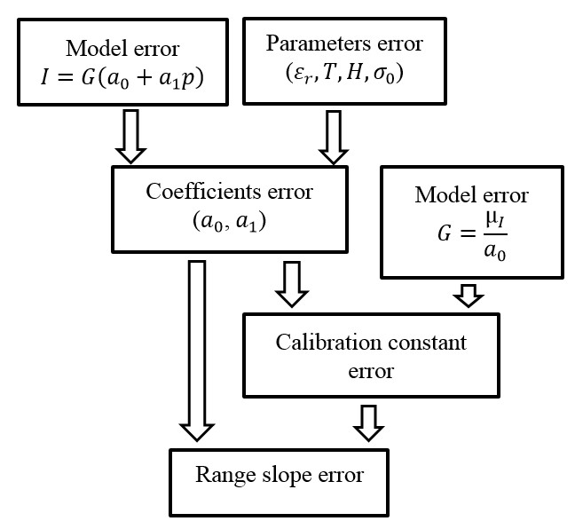
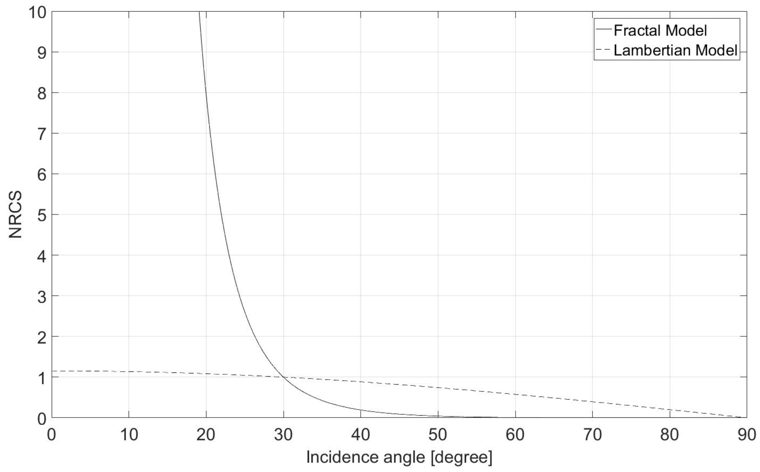
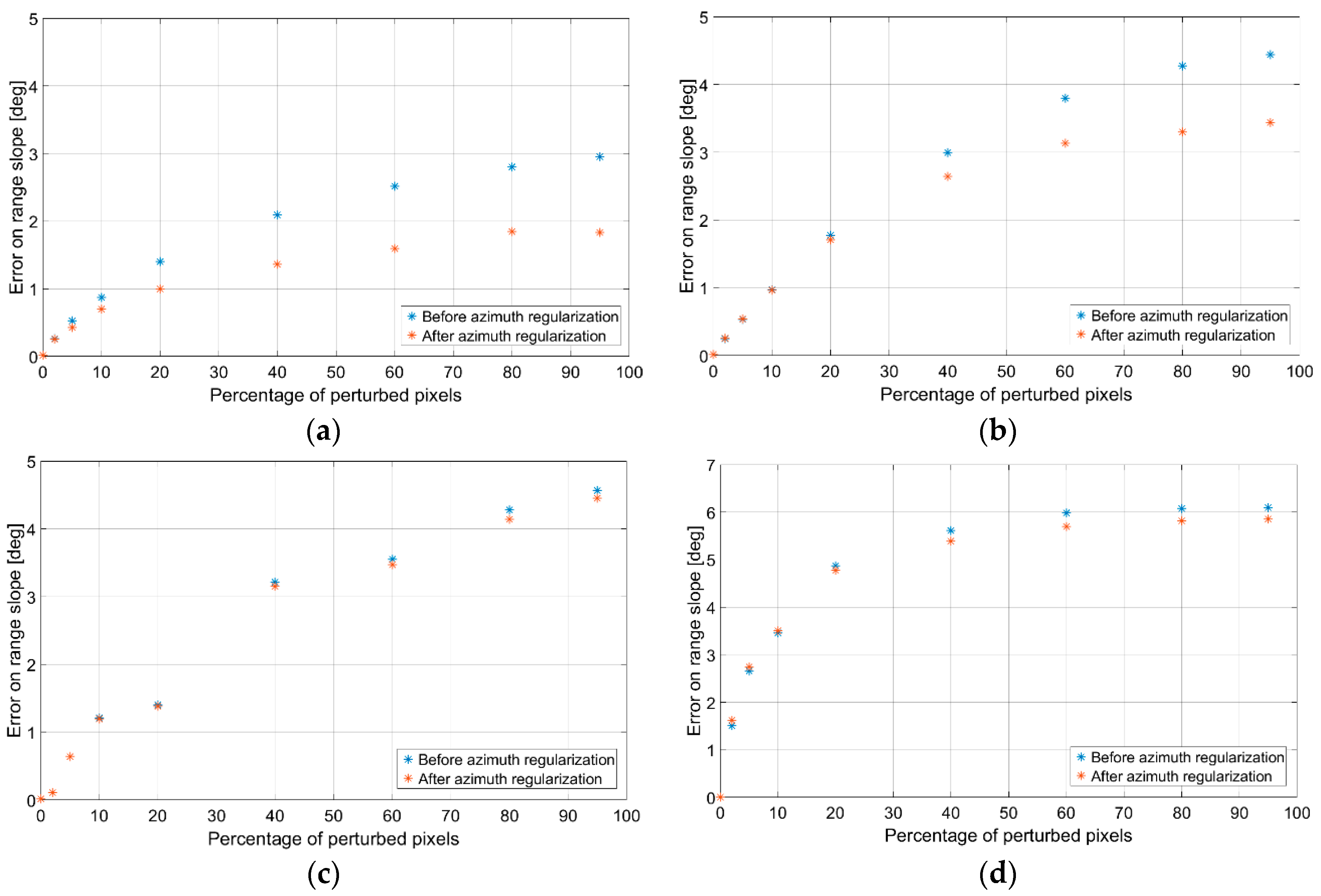
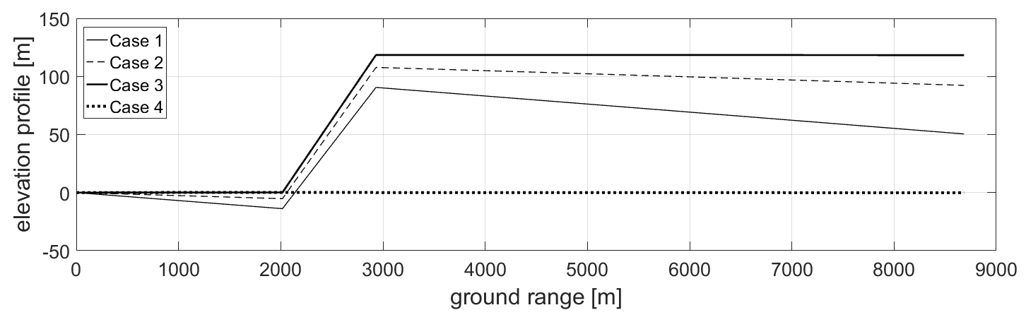
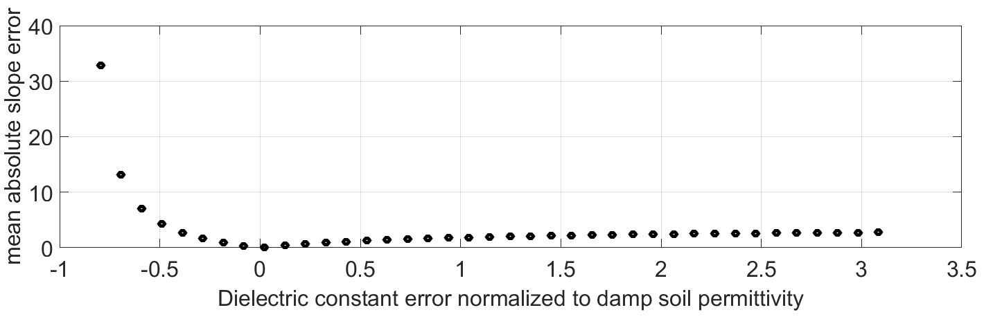
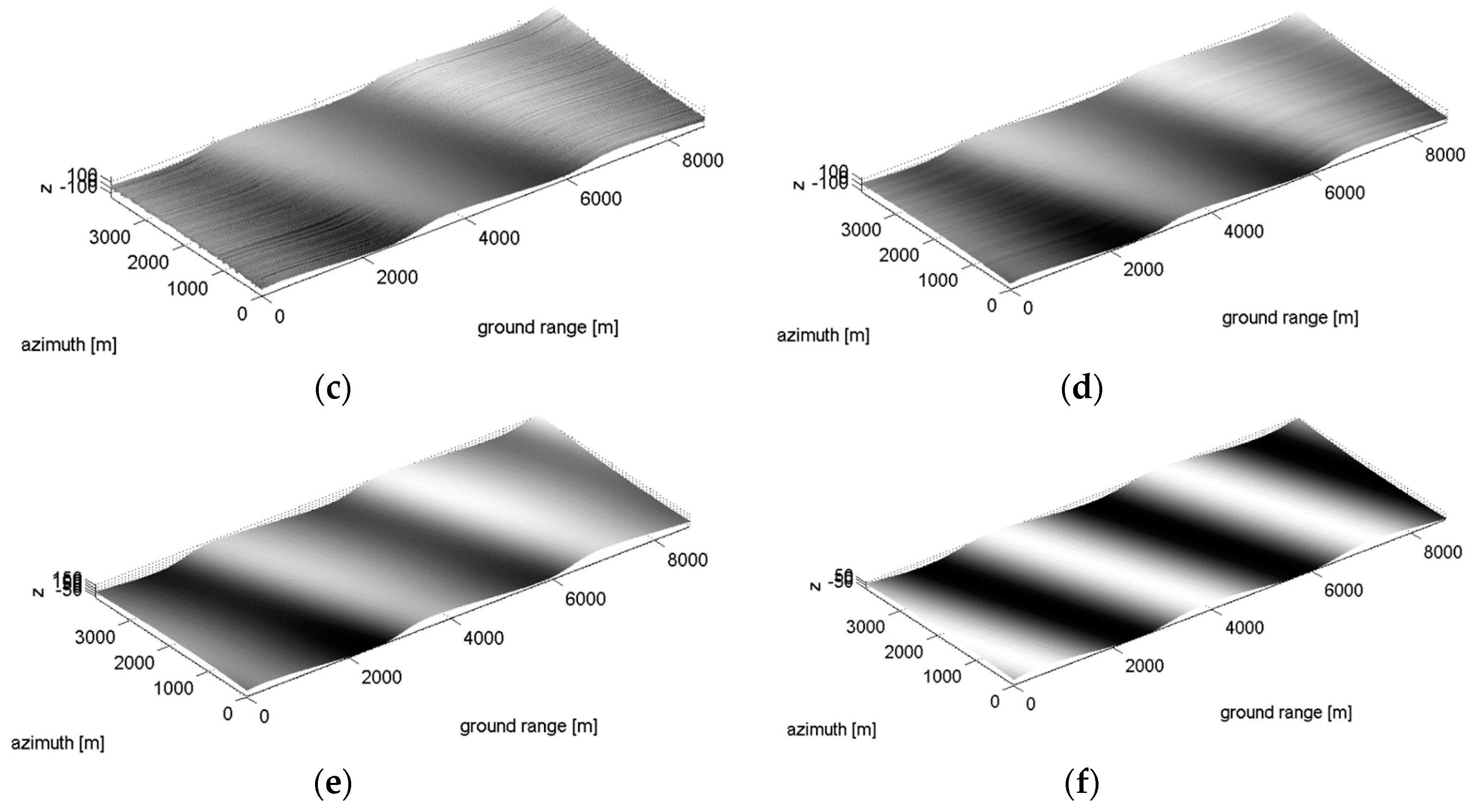
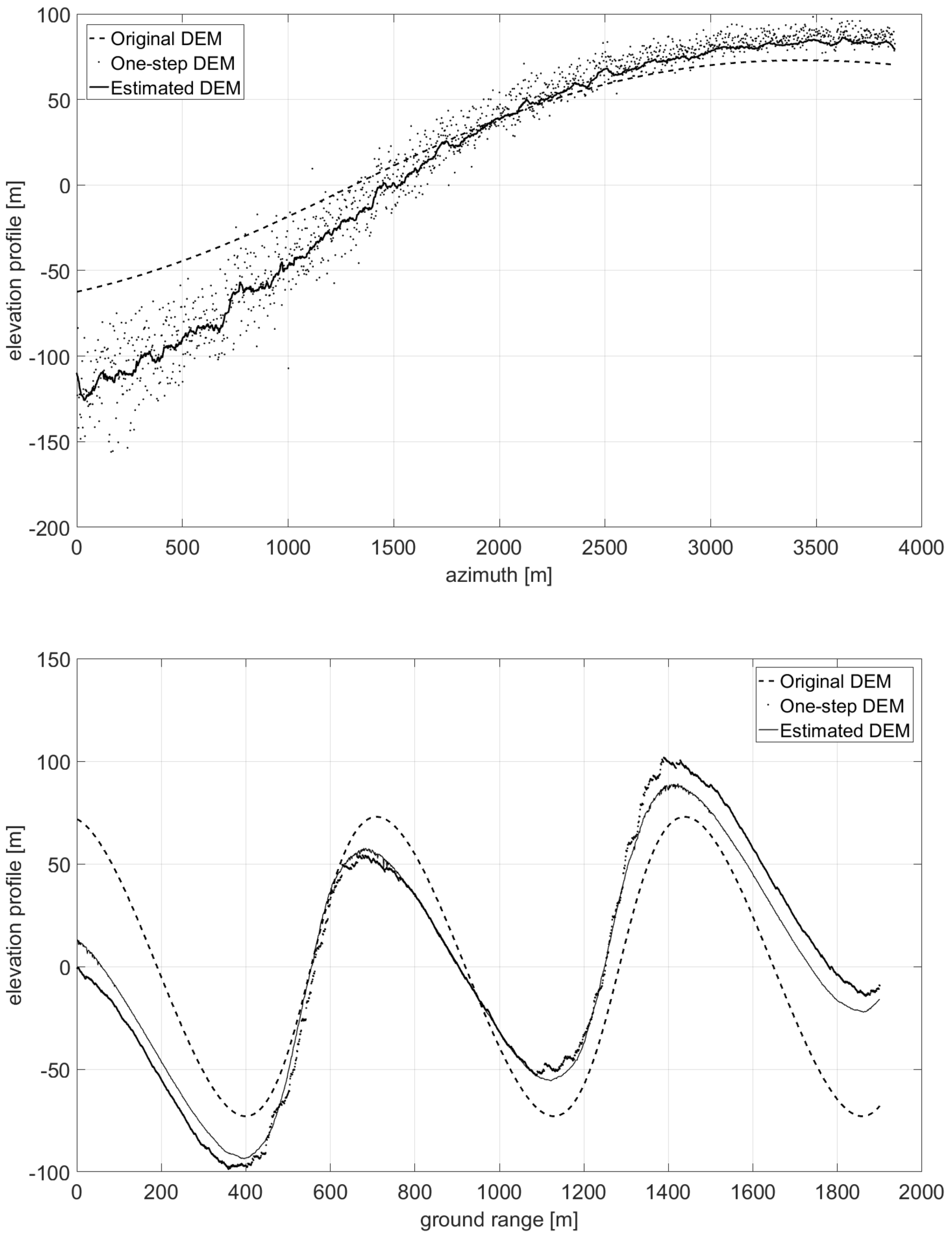
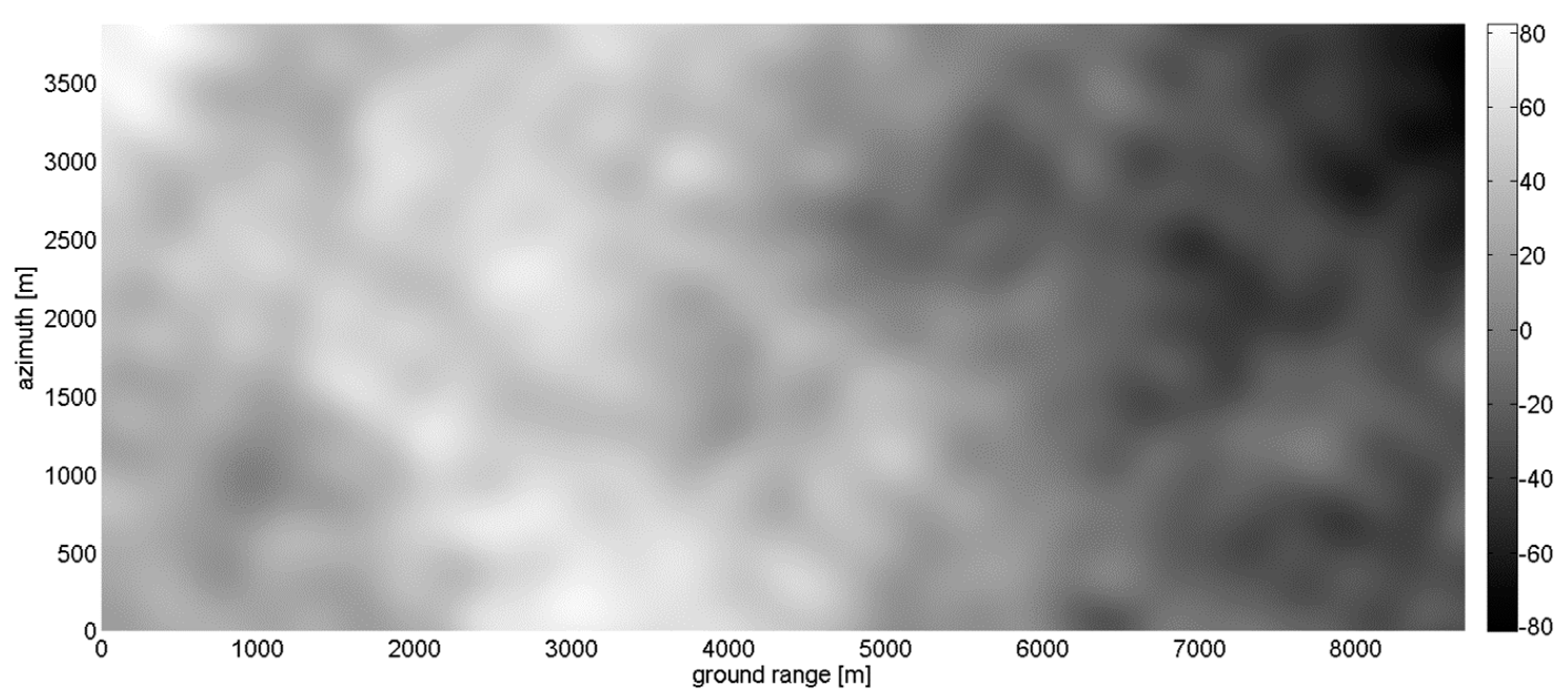
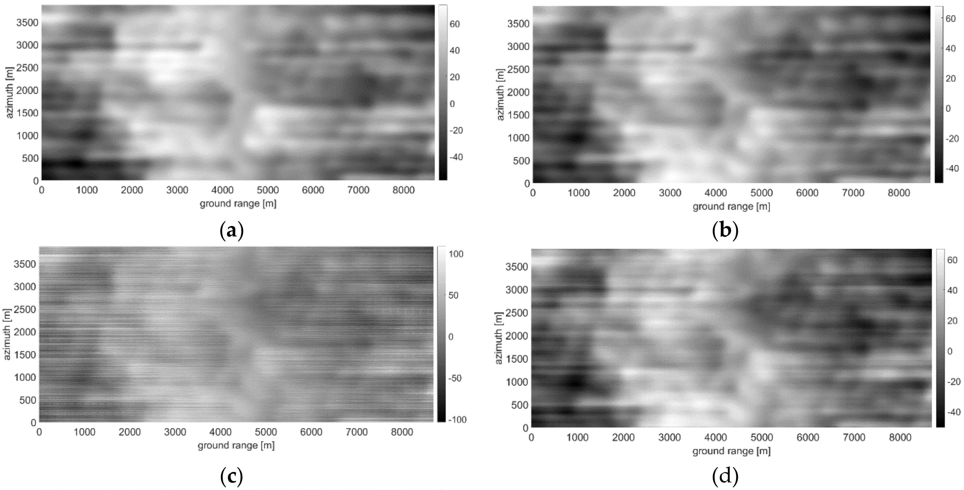
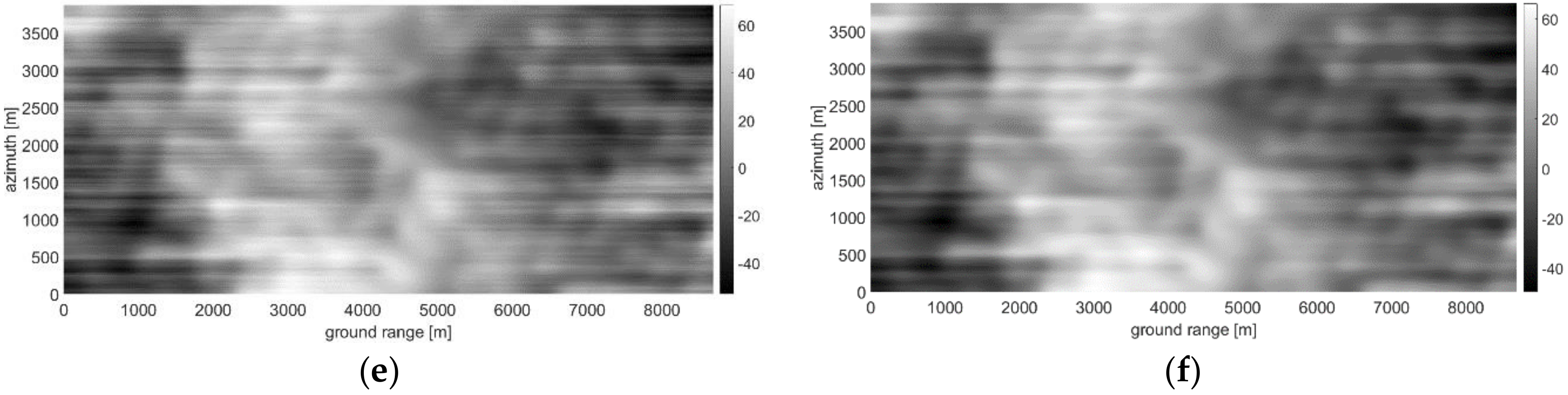
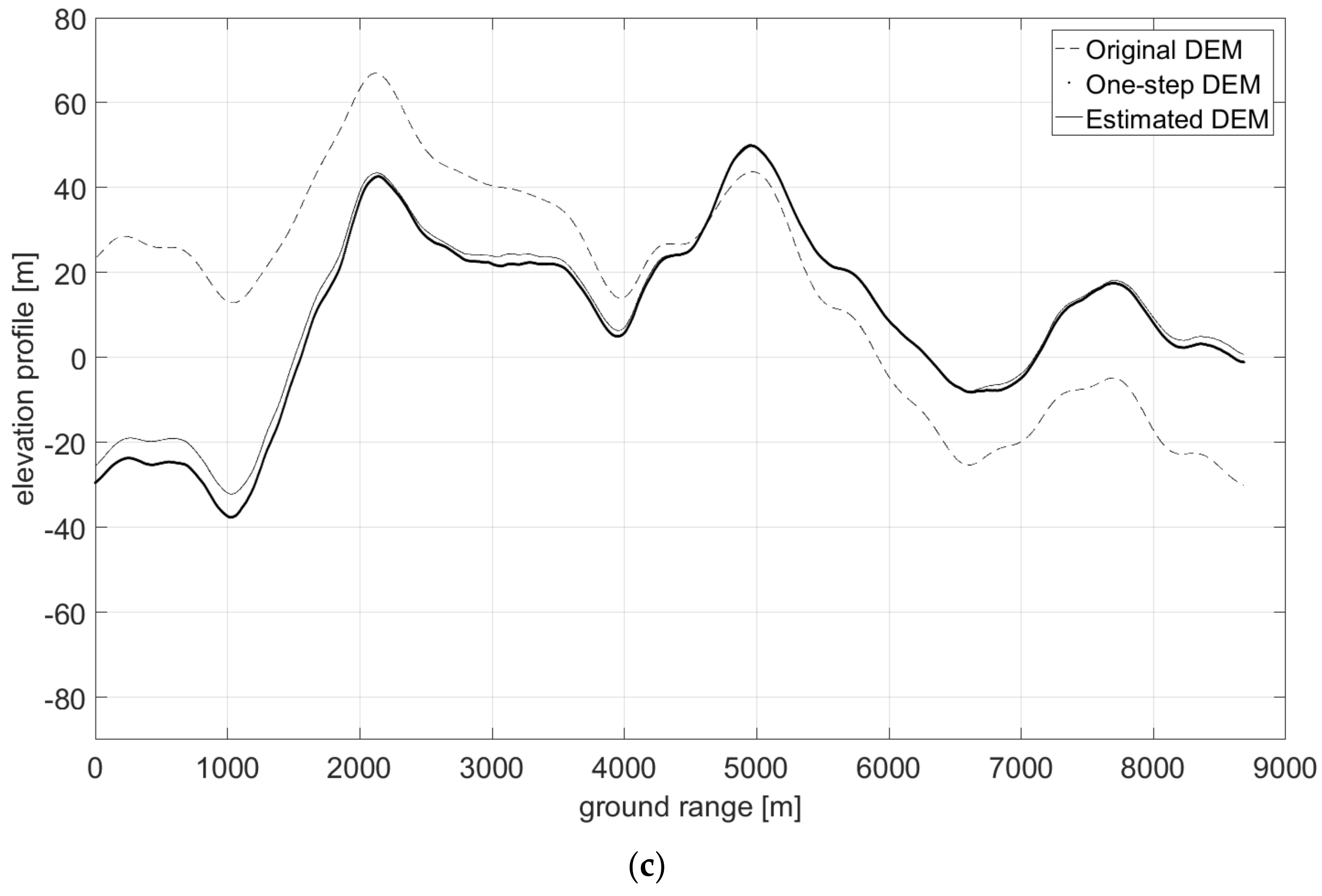
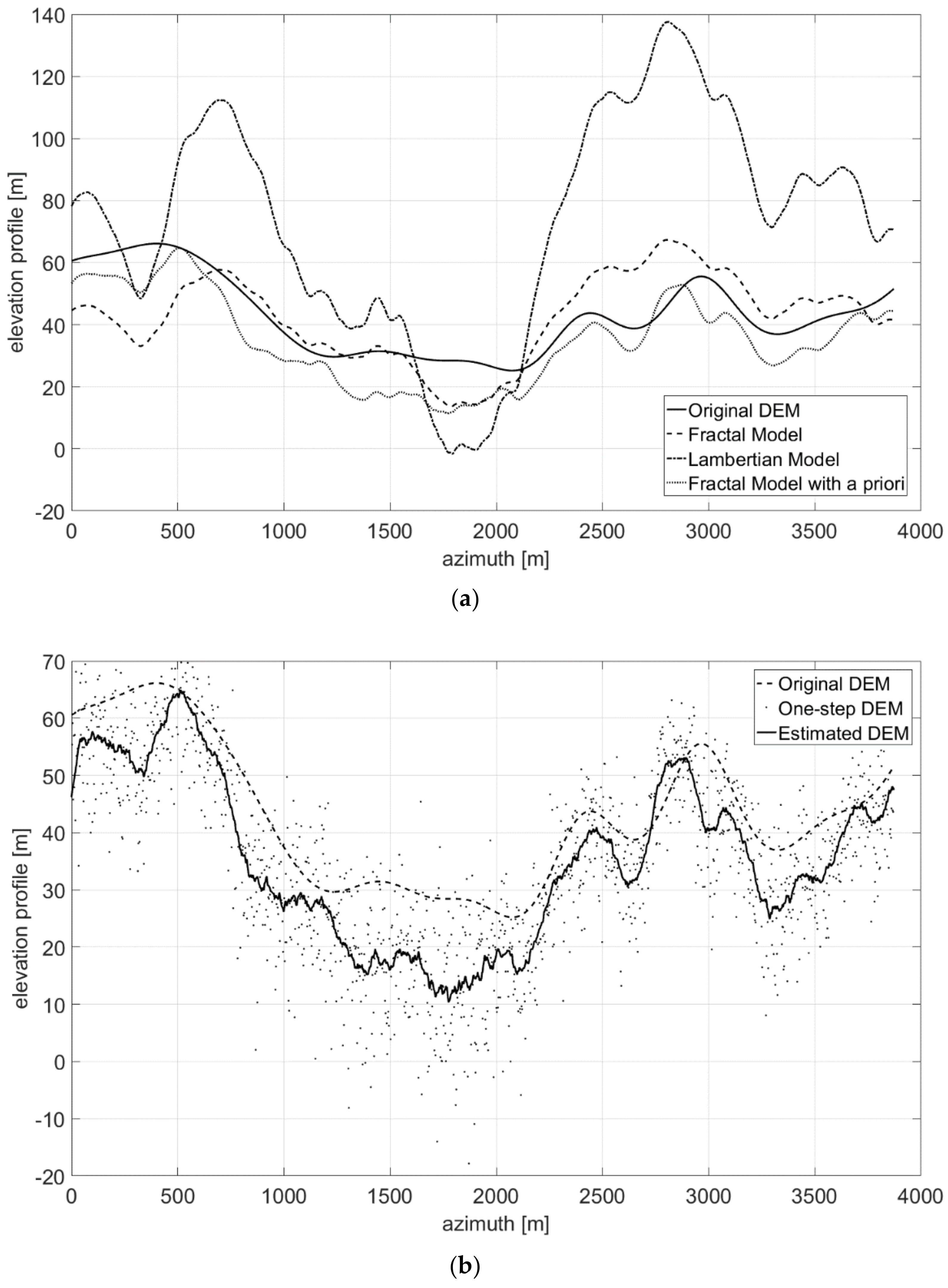
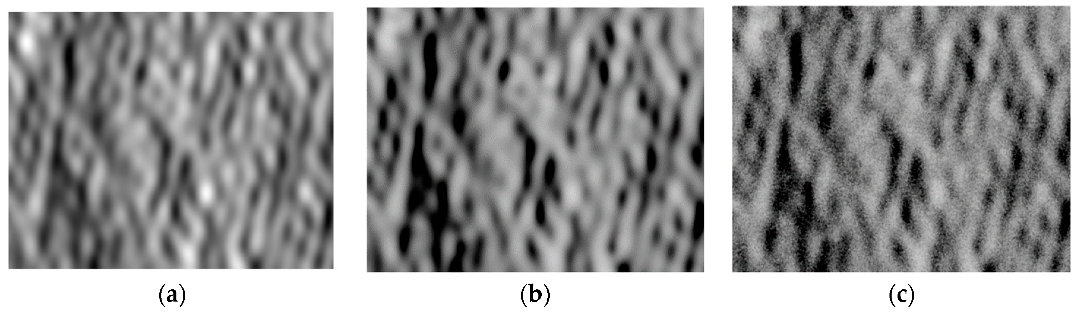
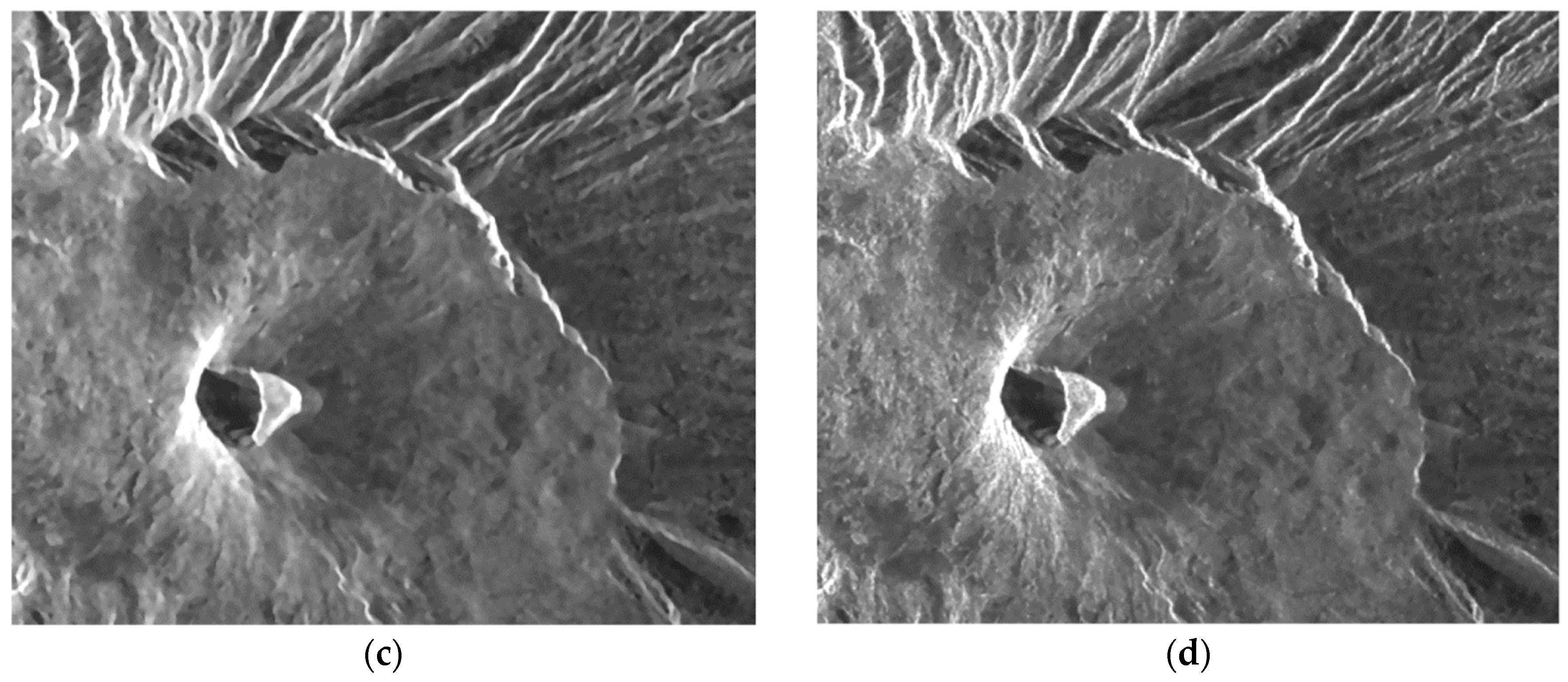
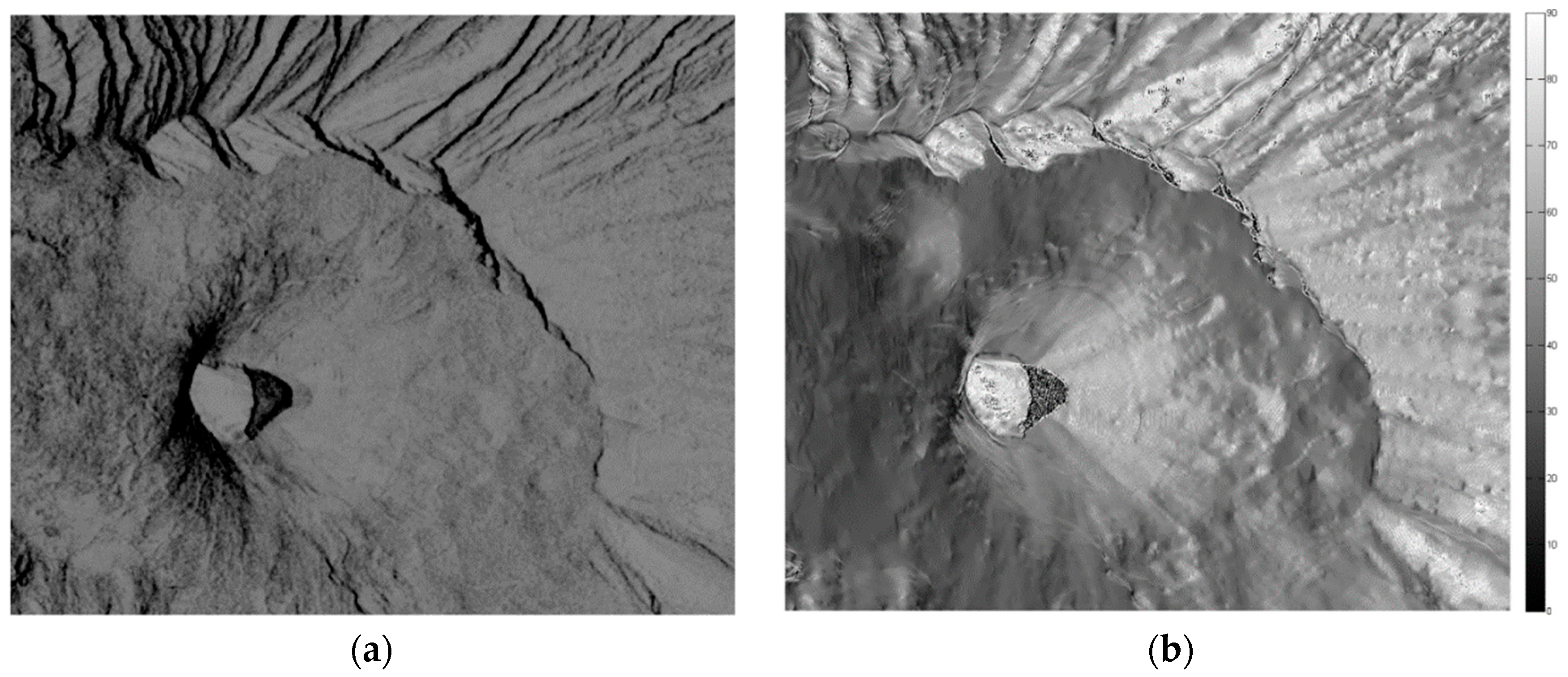
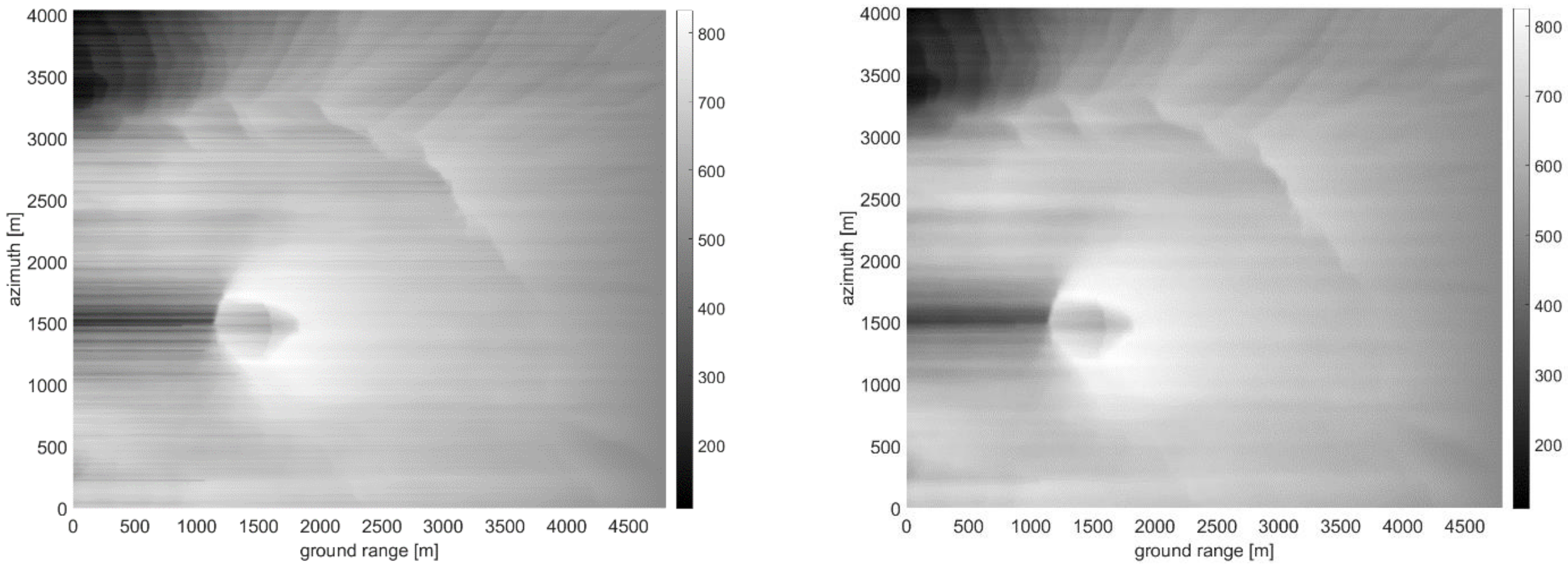
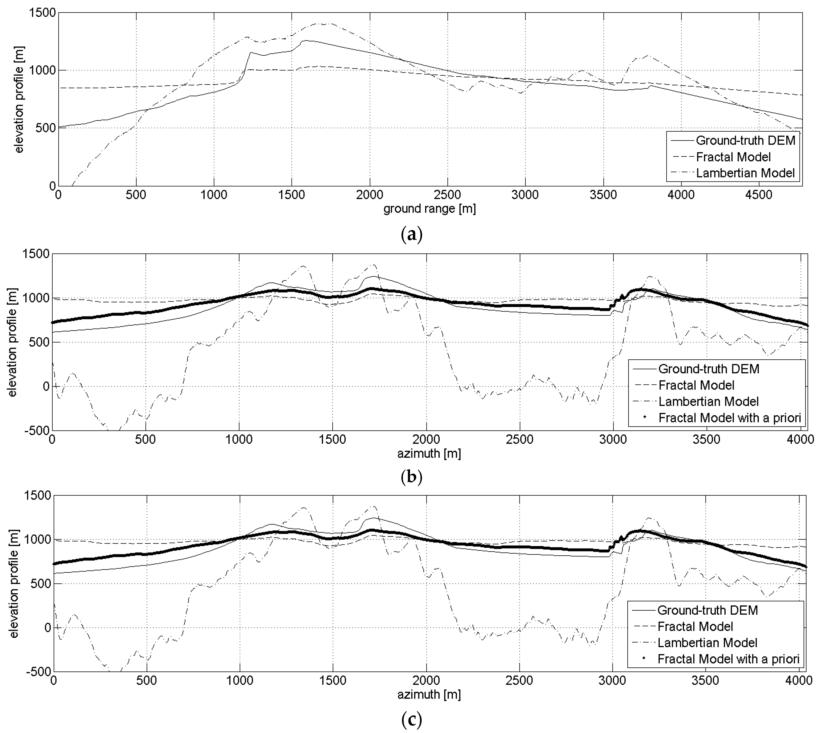
Table 1.
Quality measures for the sinusoidal DEM: speckle-free case.
| Error Magnitude | Elevation (m) | Range Slope (°) | Azimuth Slope (°) | ||||||||
|---|---|---|---|---|---|---|---|---|---|---|---|
| Median | Mean | Std dev | Median | Mean | Std dev | Median | Mean | Std dev | |||
| Before azimuth filtering | Fractal Model | 34.1 | 38.5 | 26.8 | 1.40 | 1.41 | 1.00 | 1.67 | 1.79 | 1.16 | |
| Lambertian Model | 132.9 | 150.0 | 106.1 | 10.20 | 10.46 | 5.94 | 3.73 | 5.54 | 5.08 | ||
| After azimuth filtering | Unknown starting points | Fractal Model | 33.9 | 38.2 | 26.7 | 1.41 | 1.41 | 0.99 | 1.67 | 1.65 | 0.64 |
| Lambertian Model | 132.5 | 149.0 | 105.0 | 10.07 | 10.35 | 5.89 | 2.36 | 4.66 | 4.66 | ||
| Known starting points | Fractal Model | 27.6 | 28.0 | 17.2 | 1.42 | 1.41 | 0.99 | 0.33 | 0.48 | 0.43 | |
| Lambertian Model | 124.5 | 137.2 | 94.5 | 10.07 | 10.35 | 5.89 | 0.87 | 3.21 | 4.50 | ||
Table 2.
Quality measures for the sinusoidal DEM: speckle case.
| Error Magnitude | Elevation (m) | Range Slope (°) | Azimuth Slope (°) | ||||||||
|---|---|---|---|---|---|---|---|---|---|---|---|
| Median | Mean | Std dev | Median | Mean | Std dev | Median | Mean | Std dev | |||
| Before azimuth filtering | Fractal Model | 30.0 | 35.3 | 26.3 | 2.78 | 4.23 | 4.78 | 74.46 | 63.27 | 25.34 | |
| Lambertian Model | 112.1 | 129.7 | 94.6 | 12.22 | 13.43 | 10.45 | 84.53 | 76.33 | 19.37 | ||
| After azimuth filtering | Unknown starting points | Fractal Model | 29.2 | 33.7 | 24.1 | 2.36 | 3.67 | 4.50 | 9.70 | 14.00 | 12.90 |
| Lambertian Model | 110.4 | 124.7 | 88.1 | 9.56 | 12.42 | 10.71 | 21.02 | 25.39 | 20.17 | ||
| Known starting points | Fractal Model | 23.5 | 25.2 | 16.9 | 2.36 | 3.67 | 4.50 | 9.60 | 13.86 | 12.97 | |
| Lambertian Model | 101.2 | 112.4 | 77.6 | 9.57 | 12.42 | 10.71 | 28.53 | 31.54 | 23.18 | ||
Table 3.
Quality measures for the sinusoidal DEM: without speckle.
| Error Magnitude | Elevation (m) | Range Slope (°) | Azimuth Slope (°) | ||||||||
|---|---|---|---|---|---|---|---|---|---|---|---|
| Median | Mean | Std dev | Median | Mean | Std dev | Median | Mean | Std dev | |||
| Before azimuth filtering—Unknown starting points—Fractal Model | 19.6 | 22.3 | 15.9 | 0.59 | 0.75 | 0.68 | 2.97 | 3.61 | 2.98 | ||
| After azimuth filtering | Unknown starting points | Fractal Model | 19.7 | 22.3 | 15.8 | 0.61 | 0.76 | 0.69 | 2.85 | 3.48 | 2.86 |
| Lambertian Model | 38.9 | 51.7 | 46.8 | 3.42 | 4.09 | 3.47 | 8.81 | 10.78 | 8.76 | ||
| Known starting points | Fractal Model | 17.4 | 19.9 | 14.1 | 0.61 | 0.76 | 0.69 | 2.03 | 2.79 | 2.57 | |
| Lambertian Model | 39.0 | 51.8 | 45.8 | 3.42 | 4.09 | 3.47 | 7.97 | 10.02 | 8.43 | ||
Table 4.
Quality measures for the sinusoidal DEM: speckle case; known starting points in range integration.
Table 4.
Quality measures for the sinusoidal DEM: speckle case; known starting points in range integration.
| Error Magnitude | Elevation (m) | Range Slope (°) | Azimuth Slope (°) | |||||||
|---|---|---|---|---|---|---|---|---|---|---|
| Median | Mean | Std dev | Median | Mean | Std dev | Median | Mean | Std dev | ||
| Before azimuth filtering | Fractal Model | 16.1 | 20.8 | 18.0 | 4.32 | 5.40 | 5.18 | 74.49 | 65.95 | 21.83 |
| Lambertian Model | 33.6 | 45.6 | 42.4 | 12.21 | 13.51 | 10.39 | 83.58 | 77.13 | 17.15 | |
| After azimuth filtering | Fractal Model | 17.4 | 19.7 | 14.0 | 2.93 | 4.18 | 4.07 | 7.19 | 9.28 | 7.92 |
| Lambertian Model | 27.7 | 38.0 | 35.3 | 8.01 | 10.71 | 9.37 | 18.37 | 21.31 | 15.70 | |
Table 5.
Quality measures for the sinusoidal DEM: multilook case; known starting points in range integration.
Table 5.
Quality measures for the sinusoidal DEM: multilook case; known starting points in range integration.
| Error Magnitude | Elevation (m) | Range Slope (°) | Azimuth Slope (°) | |||||||
|---|---|---|---|---|---|---|---|---|---|---|
| Median | Mean | Std dev | Median | Mean | Std dev | Median | Mean | Std dev | ||
| Before azimuth filtering | Fractal Model | 17.3 | 19.8 | 14.7 | 0.79 | 1.00 | 0.86 | 21.17 | 24.09 | 17.26 |
| Lambertian Model | 28.7 | 39.0 | 36.1 | 2.93 | 3.56 | 2.98 | 47.23 | 42.67 | 23.08 | |
| After azimuth filtering | Fractal Model | 17.6 | 19.8 | 14.3 | 0.71 | 0.89 | 0.75 | 3.43 | 4.10 | 3.76 |
| Lambertian Model | 27.9 | 38.0 | 35.4 | 2.71 | 3.30 | 2.78 | 8.59 | 10.86 | 9.14 | |
Table 6.
Quality measures for the actual multilook SAR image of the Vesuvius volcano.
| Error Magnitude | Elevation (m) | Range Slope (°) | Azimuth Slope (°) | ||||||||
|---|---|---|---|---|---|---|---|---|---|---|---|
| Median | Mean | Std dev | Median | Mean | Std dev | Median | Mean | Std dev | |||
| Before azimuth filtering | Fractal Model | 140.7 | 163.9 | 118.4 | 9.32 | 11.20 | 9.40 | 21.31 | 27.10 | 22.03 | |
| Lambertian Model | 318.8 | 501.1 | 492.0 | 24.43 | 29.61 | 21.20 | 83.39 | 79.50 | 25.65 | ||
| After azimuth filtering | Unknown starting points | Fractal Model | 140.7 | 163.9 | 118.3 | 9.38 | 11.33 | 9.51 | 12.20 | 15.08 | 12.69 |
| Lambertian Model | 312.0 | 490.8 | 481.8 | 28.55 | 33.86 | 21.73 | 60.78 | 56.79 | 27.99 | ||
| Known starting points | Fractal Model | 98.4 | 124.4 | 102.4 | 9.38 | 11.33 | 9.51 | 9.22 | 13.80 | 15.20 | |
| Lambertian Model | 307.7 | 492.3 | 498.6 | 28.55 | 33.86 | 21.73 | 60.07 | 56.13 | 28.17 | ||
© 2018 by the authors. Licensee MDPI, Basel, Switzerland. This article is an open access article distributed under the terms and conditions of the Creative Commons Attribution (CC BY) license (http://creativecommons.org/licenses/by/4.0/).
Share and Cite
MDPI and ACS Style
Di Martino, G.; Di Simone, A.; Riccio, D. Fractal-Based Local Range Slope Estimation from Single SAR Image with Applications to SAR Despeckling and Topographic Mapping. Remote Sens. 2018, 10, 1294. https://doi.org/10.3390/rs10081294
AMA Style
Di Martino G, Di Simone A, Riccio D. Fractal-Based Local Range Slope Estimation from Single SAR Image with Applications to SAR Despeckling and Topographic Mapping. Remote Sensing. 2018; 10(8):1294. https://doi.org/10.3390/rs10081294
Chicago/Turabian StyleDi Martino, Gerardo, Alessio Di Simone, and Daniele Riccio. 2018. "Fractal-Based Local Range Slope Estimation from Single SAR Image with Applications to SAR Despeckling and Topographic Mapping" Remote Sensing 10, no. 8: 1294. https://doi.org/10.3390/rs10081294
Note that from the first issue of 2016, this journal uses article numbers instead of page numbers. See further details here.