Virtual Structural Analysis of Jokisivu Open Pit Using ‘Structure-from-Motion’ Unmanned Aerial Vehicles (UAV) Photogrammetry: Implications for Structurally-Controlled Gold Deposits in Southwest Finland

Abstract

Unmanned aerial vehicles (UAVs) are rapidly growing remote sensing platforms for capturing high-resolution images of exposed rock surfaces. We used a DJI Phantom 3 Professional (P3P) quadcopter to capture aerial images that were used to generate a high-resolution three-dimensional (3-D) model of the Jokisivu open-pit gold deposit that is located in southwestern Finland. 158 overlapping oblique and nadir images were taken and processed with Agisoft Photoscan Pro to generate textured 3-D surface models. In addition, 69 overlapping images were taken from the steep faces of the open pit. We assessed the precision of the 3-D model by deploying ground control points (GCPs) and the average errors were found minimal along X (2.0 cm), Y (1.2 cm), and Z (5.0 cm) axes. The steep faces of the open pit were used for virtual structural measurements and kinematic analyses in CloudCompare and ArcGIS to distinguish the orientation of different fracture sets and statistical categorization, respectively. Three distinct fracture sets were observed. The NW-SE and NE-SW striking fractures form a conjugate geometry, whereas the NNW-SSE striking fractures cut the conjugate fracture set. The orientation of conjugate fractures match well with the resource model of the deposit and NW- and NE-trending segments of regional-scale anastomosing shear zones. Based on the conjugate geometry of fracture sets I and II, and the regional pattern of anastomosing shear system lead us to interpret an origin of gold mineralization in two stages. An early N-S or NNW-SSE crustal shortening, corresponding to the regional D4 (ca. 1.83–1.81 Ga) or pre-D4 (ca. 1.87–1.86 Ga) Svecofennian tectonic event(s) that produced anastomosing shear zones. Subsequent E-W directed D5 contraction (ca. 1.79–1.77 Ga) partly reactivated the anastomosing shear zones with the formation of conjugate system, which controlled the migration of fluids and gold mineralization in SW Finland.

1. Introduction

With the invention and rapid development of small, lightweight, civilian unmanned aerial vehicles (UAVs), close-range, high-resolution digital photogrammetry is becoming a popular technique in geoscience mapping and applications [1,2]. Modern UAVs are time efficient in the precise imaging of relatively large, low- to high-relief topographic surfaces and bedrock at low altitudes (for example <120 m above ground level). Although UAVs have a small camera footprint on the ground as compared to satellite images, by using the SfM approach, larger areas can be covered at high resolution [3,4]. In particular, UAVs offer close range imaging of subvertical faces of inaccessible cliffs, canyon, road cuts, mountain slopes, open-pit mines, and thus provide a convenient remote sensing platform to collect ultra-high-resolution imagery over outcrops that are difficult or impossible to access [5,6]. The combined ‘structure-from-motion’ and ‘multi-view stereopsis’ (SfM-MVS) workflow allows for building high-resolution, three-dimensional (3-D) models of rock faces that can be used for virtual structural analysis of planar structures [7,8,9,10].

In this study, we have adopted the UAV-based SfM-MVS approach to generate a high-resolution 3-D model of an open-pit mine and further show how the model can effectively be useful to virtually measure different structural features on the computer, which is otherwise difficult in terms of mine safety regulations and steep nature of open-pit faces. We used a commercially available, low-cost DJI’s Phantom 3 Professional (P3P) quadcopter (http://www.dji.com/) to capture high-resolution, low-altitude overlapping aerial images (Figure 1). The aerial images were processed in PhotoScan Professional version 1.2.4 from Agisoft LLC (hereafter referred to as PhotoScan) (http://www.agisoft.com/) to generate textured 3-D models. The 3-D models were imported in CloudCompare, which can deal with such kind of data formats, for detailed virtual structural analysis and segmentation of well-exposed surfaces. The data were further statistically categorized in ArcGIS platform.

Thus, our workflow steps are, as follows: (1) capturing aerial images with the P3P; (2) their processing in PhotoScan; (3) virtual structural and facets analysis using CloudCompare; and, (4) further categorization with ArcGIS (Figure 2). We applied this workflow for detailed structural analyses, as we illustrate with a case study of the Paleoproterozoic Jokisivu gold open-pit mine of SW Finland. However, the workflow can be equally applied in other environments, wherever gaps in the coverage of structural field data resulting from inaccessible outcrop need to be filled.

Paleoproterozoic gold mineralization in many parts of Finland, including SW Finland, is structurally controlled and it has been generally related to the episodic events of Svecofennian orogeny (1.9 to 1.78 Ga) [11,12,13,14]. However, little has been published on the temporal and spatial relationships between gold deposition and the kinematics of deformation. Detailed virtual structural analysis of part of the northern wall of the Jokisivu gold open-pit mine has allowed for us to determine the relative timing of different fracture sets that can be correlated within an array of regional scale gold-bearing shear zones in SW Finland. The localization of known gold deposits and prospects approximately matches this distribution of these regional scale shear zones and leads us to propose an origin of syntectonic gold mineralization in the region in two stages and it is discussed below. This tectono-metallogenic model potentially provides a new framework for exploration strategies in the area.

2. Unmanned Aerial Vehicle (UAV) Photogrammetry

2.1. Backgound

It has been demonstrated that by using SfM [15] and scale invariant feature transform (SIFT) [16] photogrammetric-based algorithms, a 3-D sparse point cloud model can be resolved from a series of 60–70% overlapping images [2,17]. The method involves the recognition of features that are present in multiple images and calculation of their spatial coordinates by triangulation based on intrinsic (e.g., focal length) and extrinsic (pose and orientation) camera parameters [18]. A much higher-resolution and dense point cloud model can be reconstructed from the sparse point cloud by multi-view stereopsis (MVS) image-matching algorithms [19,20].

The quality of the image depends on a number of factors, such as camera (sensor size, sensor type, sensor resolution), lens, and camera settings (ISO, aperture, shutter speed). Whereas, the quantity of photogrammetric data, accuracy and aerial coverage are limited by technical factors, such as aircraft maximum flight time and speed, remote control transmission range, camera axis to control vertical, inclined and horizontal orientations of the lens with respect to the Earth’s surface, overlapping ratio, UAV hover effects, and weather conditions. Image sharpness and quality benefit substantially from camera stabilization during flight. Additionally, modern UAVs resolve time synchronization between the camera shutter and on-board GPS and can produce geotagged images.

SfM builds on the principle of generating a 3-D spatial point cloud from a set of unconstrained overlapping two-dimensional (2-D) images that have been taken from different viewpoints. Camera parameters, camera positions, and camera orientations are automatically solved for each image [21]. Key points that have been matched in overlapping images allow for generating a sparse point cloud, which is only possible for stationary objects. The procedure is generally referred to as the bundle adjustment [21,22]. A subsequent dense point could model can be generated by increasing the number of spatial 3-D points while using MVS algorithms, resulting in a high density point cloud compared to the initial point cloud derived from the feature matching process based on SIFT. The model can be georeferenced using GCPs, camera locations (geotagged images), or both [23].

PhotoScan software, which is used in this study, is based on SfM-MVS algorithm automatically detecting a suite of tie points in overlapping multiple image pairs, and in turn, recognizes 3-D positions and orientation of the camera, and 3-D location of each feature in the images to generate a dense 3-D point cloud. The dense point cloud forms the basis to produce the orthomosaic, digital elevation model (DEM), and textured mesh. The latter can be imported into any commercial or open source 3-D modelling software packages, such as GEOVIA Surpac (Dassault Systèmes, Vélizy-Villacoublay, France), GOCAD, or CloudCompare for quantitative analysis.

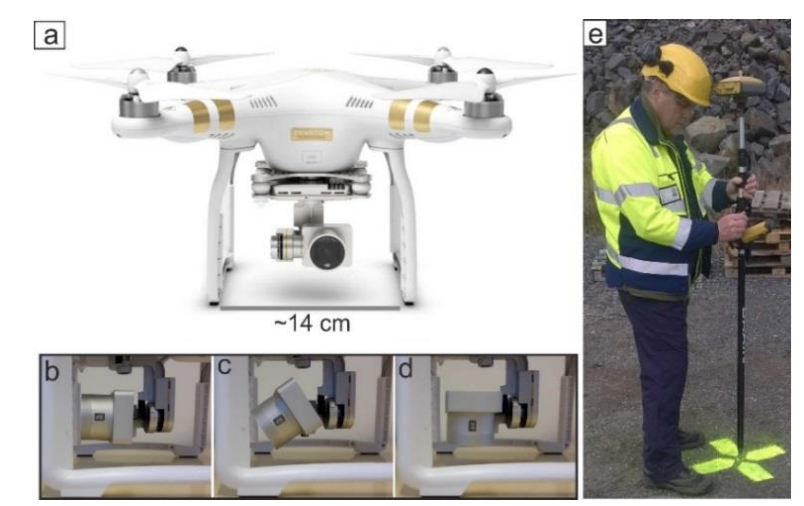
2.2. P3P Aerial Platform

The P3P is a 4-rotor micro-drone quadcopter with a user-friendly remote control, an electronically stabilized digital camera (12 megapixel resolution), GPS, and a maximum flight time of 23 min (Figure 1). The on-board GPS in the aircraft allows for embedding location information in each image and can be used for direct georeferencing [23,24]. An important feature of the P3P is its 3-axis (pitch, roll, yaw) electronic gimbal stabilization technology, which keeps the camera steady and in optimal level during flight or windy conditions (not over 10 m/s), yielding blurred-free images. The gimbal can tilt the camera vertically within 90° range allowing for the operator to collect oblique or nadir imagery (Figure 1). The transmission distance from the remote control is approximately 2000 m.

P3P comes along with the DJI Go application to remotely capture high-quality still images. The DJI Go application allows for the pilot to see real-time video footage, along with having full aircraft and camera control. Before flying the aircraft, it is obligatory to check the legal flight limitations and requirements from the local authorities. In our case, we followed Trafi regulations of Finland. We recommend that the new users should follow DJI flight video and the safety tutorials available on their website.

2.3. Image Acquisition and GCPs

In this study, images were acquired maually with a camera position orthogonal to the surface with an effective overlap of >80%. The photographic overlap was estimated with the grid lines available on the DJI Go application. Additional oblique images were taken to improve the quality in building the DEMs [25]. Images were captured during an overcast day for uniform lightening on the surface (Figure 3). The GPS information and camera parameters were embedded in each image as EXIF (Exchangeable Image File) metadata tags. The EXIF tags provide a real-world coordinate system to sparse- and dense-point clouds in the PhotoScan, resulting in thousands of real-world coordinates that are linked to points in each image, and allowing for the images to be orthorectified.

GCPs provide accurate georeferencing to the 3-D geometry [4,23] and can be used to assess the model in a case of direct georeferencing [24]. A minimum of three GCPs are required, however, depending on the size of the area and accuracy constraints, a uniform distribution of more than three GCPs are preferable [26]. In this study, ground measurements were performed with a Topcon HiPer^® RTK (Real-Time Kinematic) receiver that allows cm-accuracy along with the FC-200 field collector and TopSURV application (Figure 1e). The spatial accuracy of the instrument is lower than 10 to 30 mm in all dimensions. GCPs were evenly distributed around the scene. Each GCP is made from a 0.5 × 0.5 m size plastic template and sprayed with a luminous yellow color so that the centre point became always distinct for a precise GCP identification (Figure 1e). Eleven signals were placed around the mine pit (Figure 3a), seven were used as control points (

Table 1. Errors in X (easting), Y (northing), and Z (altitude) along control points.

Control Points	X Error (cm)	Y Error (cm)	Z Error (cm)
3	−1.6	1.3	−2.4
4	−0.8	0.1	9.2
6	3.2	−0.8	−7.3
7.1	0.5	0.9	−0.2
13	−1.1	−1.2	0.7
2	2.3	−1.7	−3.7
9	−2.6	1.5	3.5
Average	2.0	1.2	5.0

), and four as check points (

Table 2. Errors in X (easting), Y (northing), and Z (altitude) along check points.

Check Points	X Error (cm)	Y Error (cm)	Z Error (cm)
5	1.0	2.3	−6.5
10	0.3	−0.3	−9.2
11	−3.5	3.1	−2.6
8	0.3	2.7	−4.1
Average	1.8	2.4	6.1

). Whereas, the known length and width of the dome-shaped warehouse on the western side of the scene is used to further compare the distances with the model (Figure 3c).

3. Jokisivu Gold Mine Case Study

The Jokisivu quartz vein-hosted gold deposit is located ~8 km southwest from the town of Huittinen in southwestern Finland (Figure 3a) and is operated by Dragon Mining Ltd. The deposit lies within the Pirkkala Au area [12] and in the poorly-defined border zone of the Pirkanmaa and the Häme tectonic belts, which developed during the 1.9–1.8 Ga Svecofennian orogeny [14]. Most of the gold occurs as free grains in quartz veins and can be related to pyrrhotite, arsenopyrite, and tellurides [27]. The bedrock of the Jokisivu area consists of foliated granodioritic to tonalitic gneisses, mica gneisses, and minor mafic to intermediate volcanic rocks [14,27]. The mining of the Kujankallio open pit commenced in 2009 and underground development started in 2010 (Figure 3b). The ore bodies are composed of auriferous quartz vein arrays that are controlled by brittle-ductile shear zones that are interpreted as part of a regional-scale NW-SE trending shear system [12]. The proved and probable ore reserve are estimated around 500,000 tons at 3.6 g/t gold for 57,600 ounces as per December 2016.

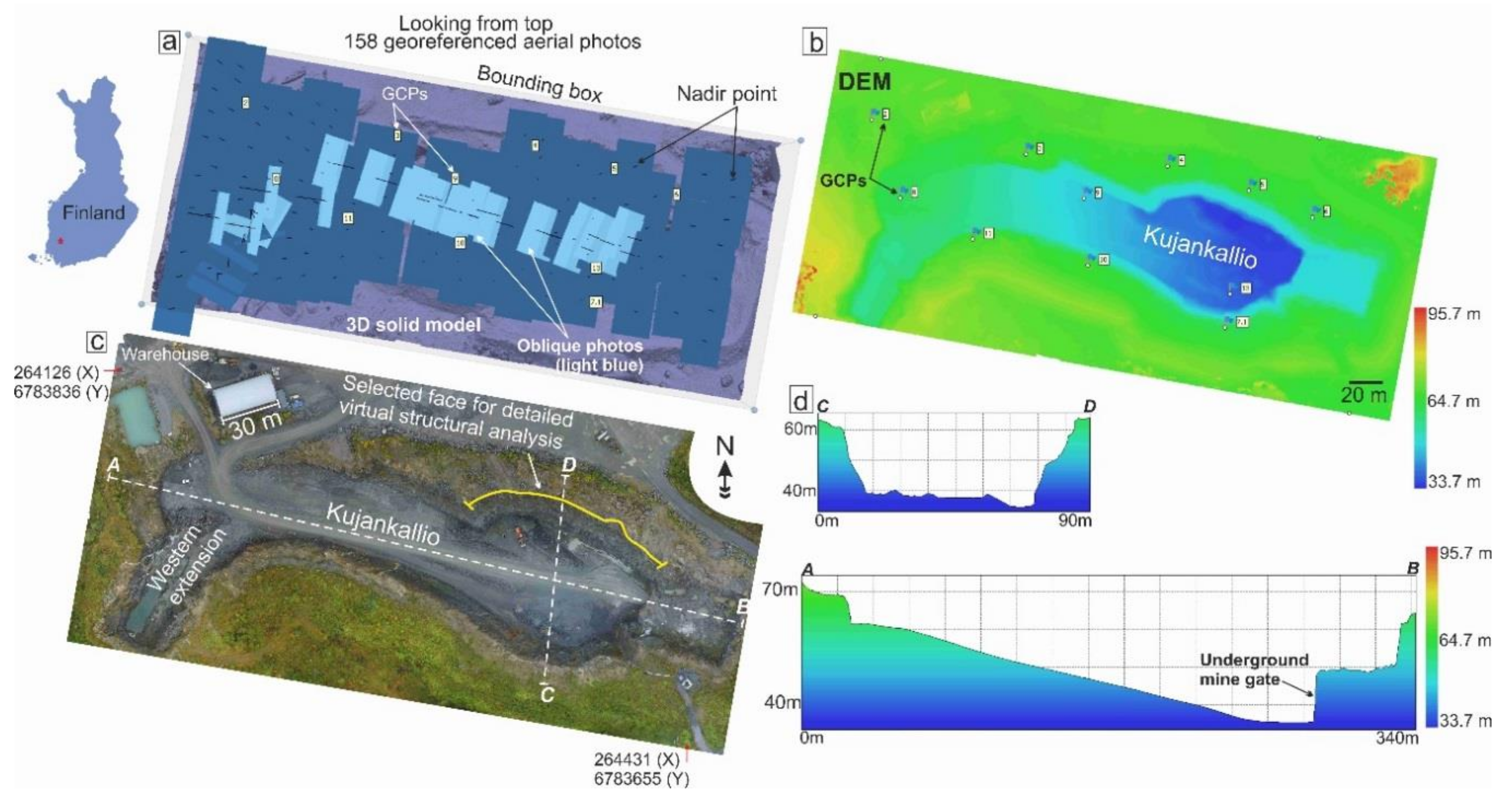
3.1. Kujankallio Open-Pit UAV Photogrammetry

During a manual flight at an altitude of ~79 m above ground surface, 158 images were captured using the P3P quadcopter on 22 April 2016 (Figure 3a). All of the images were taken in a static aircraft position before moving to the next point on the aerial route. An area of about 0.0598 km² was covered with a ground resolution of 2.86 cm/pixel. The total flight time was ~32 min (1.5 batteries). All the images were processed with an Intel^® Core™ i7-6920HQ CPU (2.90 GHz, Dell Precision, Finland) workstation with 64 GB RAM, 64-bit Windows 7 operating system and NVIDIA Quadro M2000M display adapter.

At the start, all images were imported and the picture quality was estimated using PhotoScan (Agisoft LLC, St. Petersburg, Russia) in order to detect and remove blurry images. The quality check function estimates the quality based on the sharpness level of each image. All images passed the quality test with values ranging from 0.82–0.89 out of 1. According to the PhotoScan recommendation, images producing values <0.5 should be discarded or disabled from the subsequent photogrammetric processing.

The 3-D reconstruction is a four-step process: image alignment, dense point cloud reconstruction, 3-D mesh generation, and finally, texture computation. The 3-D model can be georeferenced after the image alignment step by placing markers on photos where GCPs are located. The workflow starts with the photo alignment to find the camera positions and orientation of each photo. Photoscan estimated 75,927 tie points for sparse point cloud. The images were aligned with the ‘high’ accuracy setting and the pair pre-selection was set to the ‘reference’ mode. Reference mode allows for speeding up the feature-matching process when dealing with geotagged aerial images, as in this case taken with the P3P. The subsequent dense point cloud was reconstructed using ‘high’ quality setting and ‘mild’ depth filtering mode. Photoscan generated 27,493,593 points for the dense point cloud. In the next step, a mesh was computed from the dense point cloud using the surface type ‘height field’ with a face count (1,832,851) limited to ‘high’.

The mesh was subsequently textured with source images in the workflow while using the ‘adaptive orthophoto’ mapping mode. In this mapping mode, the horizontal elements of the model are textured with the orthographic projection, whereas the steep components are parameterized using the ‘generic’ mapping mode [18]. The total processing time of the workflow was about 2 h; however, it could vary depending on the computer specifications. A DEM (5.73 cm/pixel) was generated using the dense point cloud as a source data with a point density of 305 points/m². Finally, a high-resolution orthomosaic (2.86 cm/pixel) was produced with color correction disabled (Figure 3). Average errors calculated from seven control points are 2.0 cm in the X direction (easting), 1.2 cm in the Y direction (northing) and 5.0 cm in the Z direction (vertical) (Table 1), whereas average errors on four checkpoints are 1.8 cm in the X direction, 2.4 in the Y direction, and 6.1 in the Z direction (Table 2), along with root mean square errors (

Table 3. Control and check points root mean square errors (RMSE).

	X Error (cm)	Y Error (cm)	Z Error (cm)
Control points (7)	1.9	1.1	4.9
Check points (4)	1.8	2.3	6.1

). In addition, the accuracy was also assessed by comparing the actual dimensions (length and width) of the known objects on the ground with the measurements in the image. For example, the actual length and width of the dome-shaped warehouse on the western side of the open pit is 30 × 15 m, versus ~29.89 × 14.93 m in Photoscan, demonstrating minimal errors in the model. PhotoScan allows many quantitative analyses using DEM image including distance, area and volume measurements, and the generation of profile lines. The 2-D profiles across and along the open pit provide useful third dimension information on pit-wall slope angles (Figure 3d).

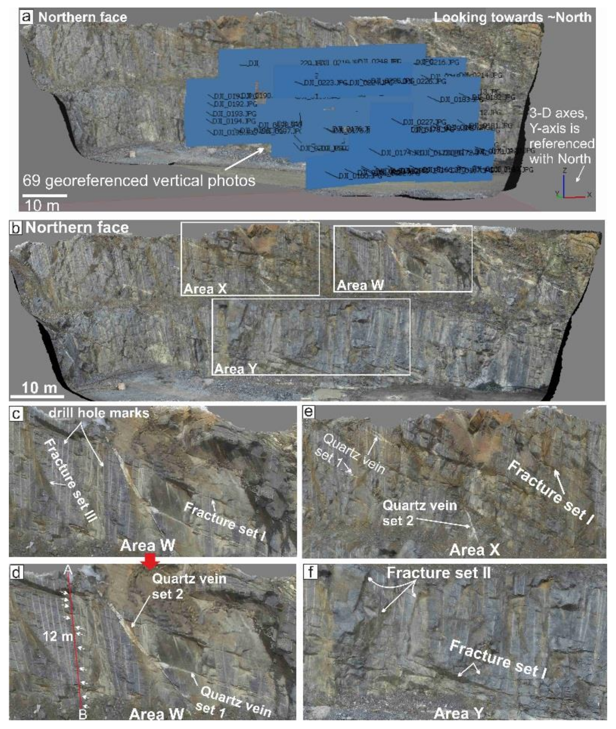
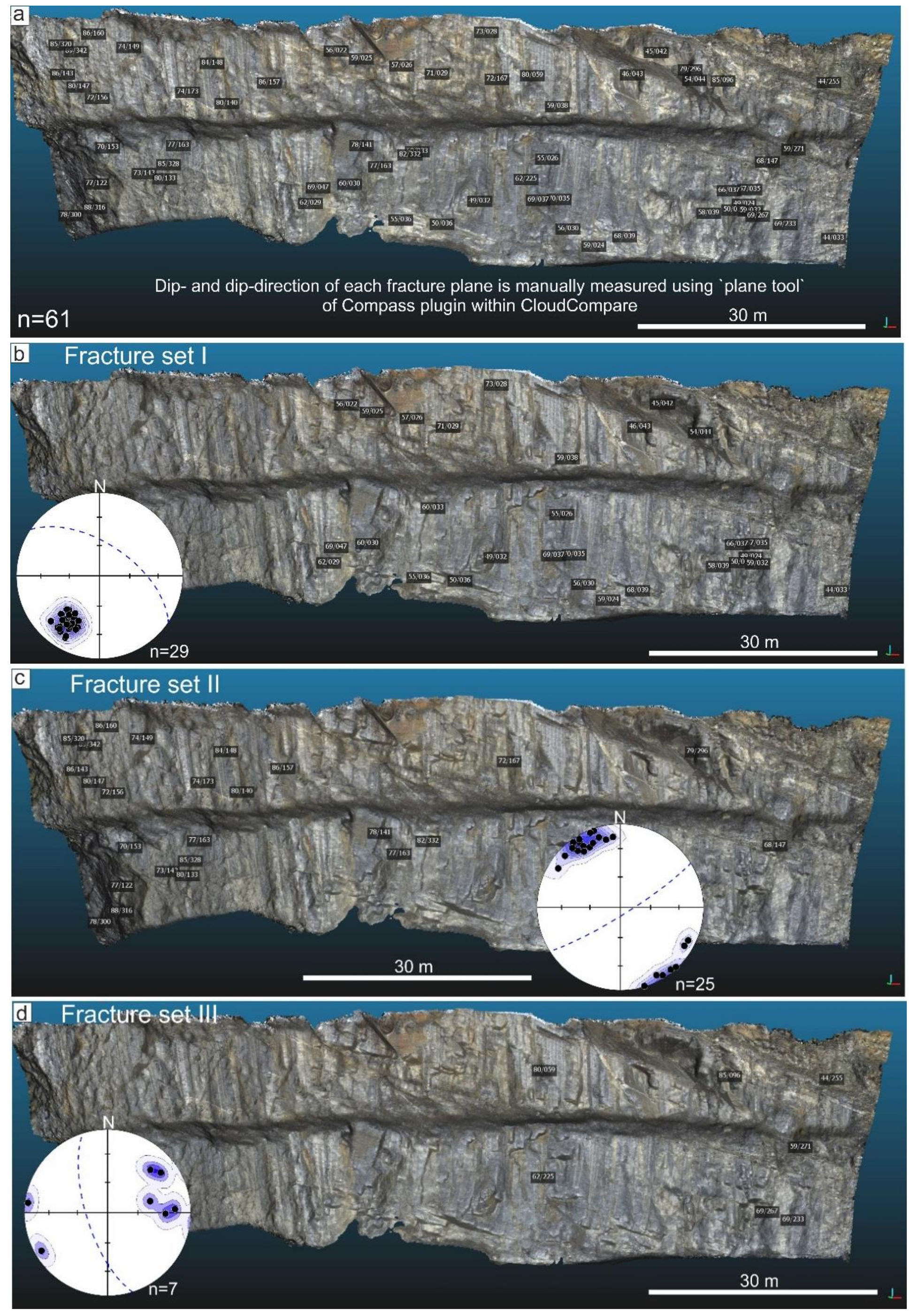
3.2. Northern Face Wall UAV Photogrammetry and Structural Analyses

For virtual structural measurements on a well-exposed part of the northern face of the open pit, we applied the same digital photogrammetry workflow as outlined above. The selected face section is ~100 m wide and ~33 m high and exhibits well exposed fracture surfaces (Figure 4).

The face is divided into upper and lower parts by a ~5 m wide bench. 69 images were manually taken in less than 12 min with a >80% overlap using P3P (Figure 4a). In order to image the steep face at a high resolution, the camera was kept at a horizontal orientation (Figure 1b) and maintained a distance of ~30–40 m to the face. All of the images were imported into the PhotoScan and passed the initial image quality check (0.85 to 0.91 out of 1). The high resolution of the model allowed detailed structural analysis of the exposed fracture planes, and is described below (Figure 4b–f).

The orthorectified image yielded a resolution of 1.45 cm/pixel. The 3-D model was imported and registered in the CloudCompare open-source software (http://www.danielgm.net/cc/), to virtually extract the orientation of planar surfaces both manually and automatically. For manual virtual measurements of planar structures, we used ‘Compass’ plugin [28] (Figure 5). 61 fracture sets were measured on well-exposed fracture planes while using the ‘Compass’ toolbox. ‘Facet’ plugin was applied to further extract planar data from the point could [29]. The method applies a least square fitting algorithm using either ‘Kd-tree’ or ‘fast-marching’ front propagation methods. We adopted the ‘Kd-tree’ feature for fracture segmentation as it recursively subdivides the point cloud in smaller planar patches and then fuses them based on similar orientation to yield fracture planes. Further categorization was applied using ‘Stereogram’ tool to interactively filter facets by orientation (dip/dip direction). The interactive filter allows for the user to compute dip- and dip-direction in angular steps. The results of the ‘Facet’ analyses were exported as a shapefile for ArcMAP (10.4.4) to classify the data into dip direction using different color palettes along with each facet value shown on the surface. The three-dimensionality, high fidelity, and resolution of the face allowed for us to thoroughly examine the structural elements down to centimeter scale.

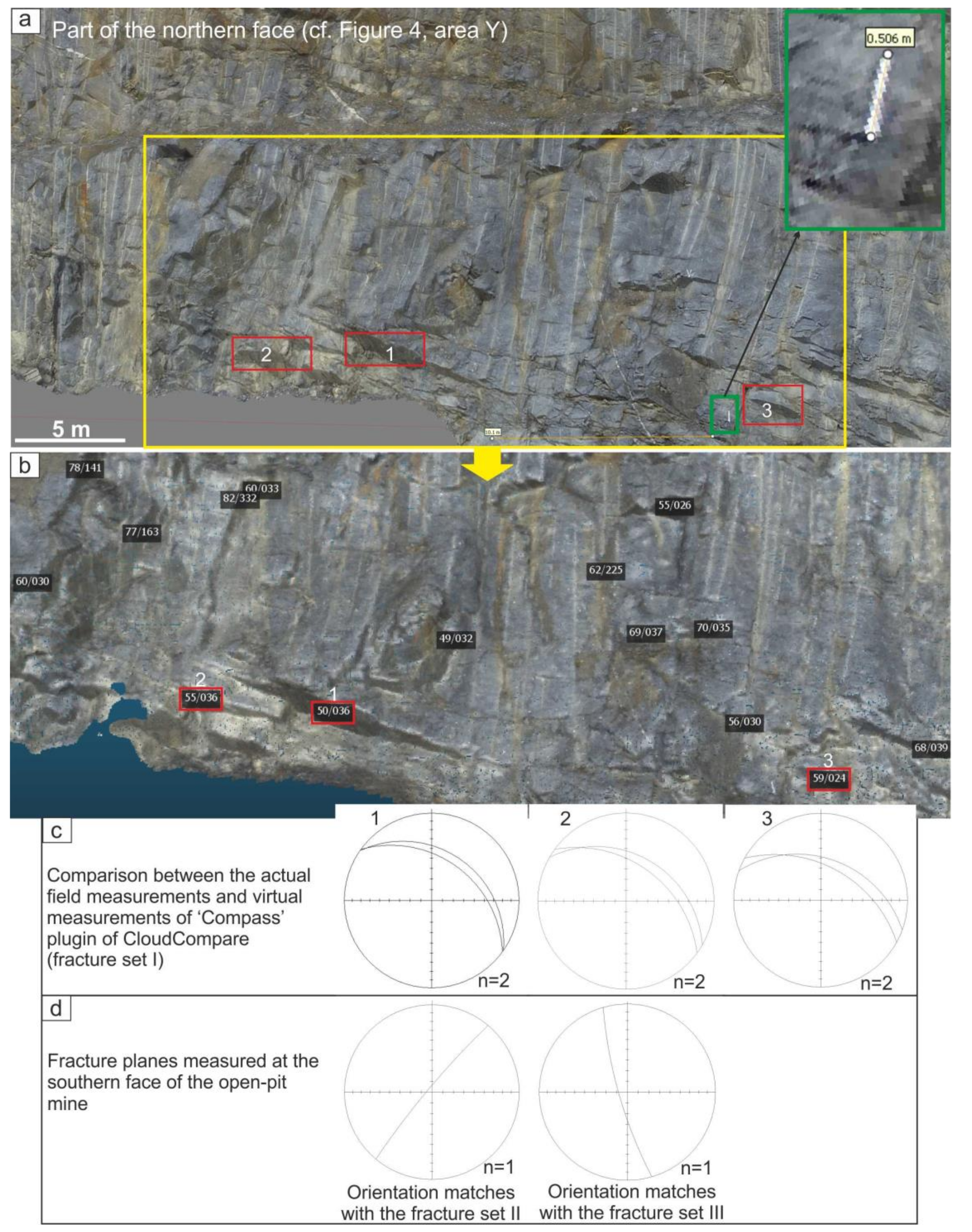
3.3. Comparison of ‘Compass’ Tool and Field Measurements

Close examination of areas labeled W, X, and Y (Figure 4) reveal three fracture sets (denoted I, II, and III) and two quartz-vein sets (labeled 1 and 2). Fracture set I strikes NW-SE, dips moderately NE (Figure 5b), and is the dominant fracture set. For estimating errors in our virtual structural data, three reference fracture planes (red boxes in Figure 6) that were exposed at the bottom of the face were manually measured in the field using a Cocla geological compass (made by Breithaupt Kassel, Germany). The steepness of the face and mine safety regulations did not allow for taking more measurements in the field. In addition, the accuracy was also assessed by comparing the length of a scale bar that was placed at the bottom of the face before the UAV photogrammetry process (Figure 6). The actual length of the scale bar is 50 cm, whereas, the length measured in the PhotoScan and CloudCompare (Version 2.9.1) show virtually the same values of 50.6 cm, demonstrating the robustness of the model.

The stereoplots (Figure 6c) show difference in the dip angles that were measured for these fractures is 8 to 9°, and for the dip direction 4° to 6°. Fracture set II strikes NE-SW and dips steeply SE (>70°) (Figure 5c). A fracture with similar dip and dip direction (86–310) was measured manually on the southern face close to the pit floor (Figure 6d). Fracture set III strikes NNW-SSE and dips moderately to steeply WSW (44° to 86°) (Figure 5d). It matches another manually measured fracture orientation (82–254) on the southern face of the pit (Figure 6d). Two well-developed sets of quartz veins (denoted as 1 and 2) are exposed in areas W and X of the open pit (Figure 4d,e), where they can be seen to be parallel to fracture sets I and III, respectively. No quartz veins that were associated with fracture set II were found in this part of the open pit, although they are present along fracture set II on the western extension (Figure 3c). The 3-D model for area W shows further that set 2 veins cut set 1 veins (Figure 4c,d) indicating that fracture set III postdates fracture set I. Close inspection of the 3-D model (Figure 4f) and stereoplots (Figure 5b,c) indicates that both fracture sets I and II cut across each other and form an acute angle (~60°), suggesting that they formed as a conjugate pair in the same stress field. This relationship further constrains the relative timing of fracture formation, where the conjugate pair predates fracture set III.

Besides structural measurements and observations, the 3-D model allows for the estimation of fracture properties, such as frequency or density. By projecting a scan line orthogonal to fracture set I on the pit face (Figure 4d), a frequency of 0.9 fractures per meter was obtained for this set.

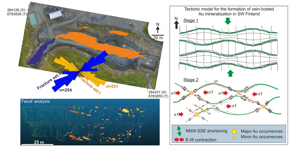
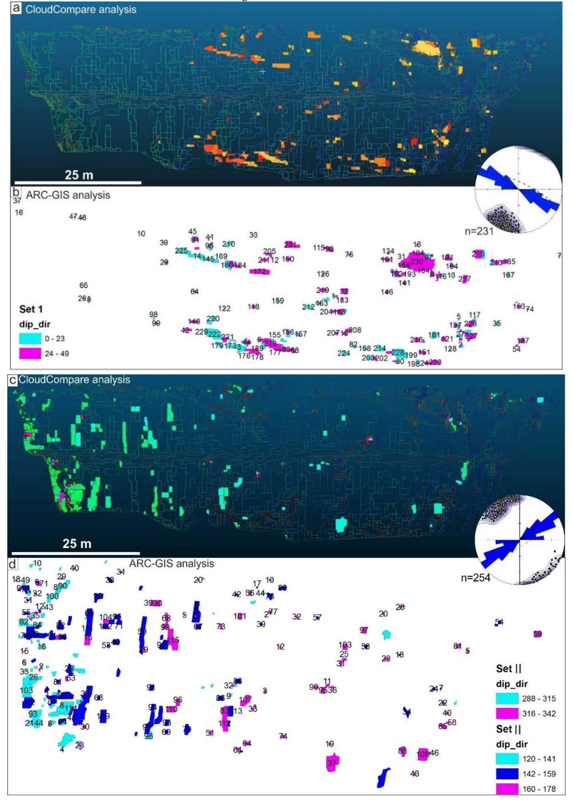
3.4. ‘Facet’ Analysis

Orientation of fractures was extracted directly from the shape of the dense 3-D point cloud. The different orientations of fracture sets were filtered with the ‘Stereogram’ plugin (Figure 7). 231 fractures were obtained for set I, 254 for set II, and 283 for set III. ‘Facet’ segmentation allowed for a visual estimate of the distribution of fractures sets across the selected pit wall in addition to quantitative dip and dip direction data that is in agreement with the orientation that was measured with the ‘Compass’ plugin (Figure 5 and Figure 7). Fracture set I is predominantly localized on the eastern half of the wall, whereas fracture set II dominates on the western side. Fracture set III is mostly restricted to the eastern side of the wall (Figure 7e,f).

3.5. ArcGIS Analysis

After segmentation in CloudCompare, ‘Facet’ results were exported as a shapefile for ArcMap (version10.4.4) analysis (Figure 7b,d,f). Data were classified into dip-direction range for their spatial distribution with respect to the north using different color palettes along with each facet numerical value. This statistical categorization provides a better visual estimate of the relative distribution of different fracture sets and their respective spatial orientations. Fracture set I appears uni-directional and dominantly dipping towards NE, whereas the majority of fracture set II planes are dipping towards SE. Fracture set III is bi-directional and fracture planes are dipping either towards ENE or WSW/WNW (Figure 7).

4. UAV Data and Structural Interpretations

In this paper, we have demonstrated a workflow from photogrammetric data acquisition using P3P followed by processing and 3-D model generation using Photoscan and segmentation of structural data using CloudCompare and ArcMap. We have linked the pre-existing methods in a sequence to tackle mapping of inaccessible rock faces.

Virtual structural analyses allow for us to digitally measure dip-angle and dip-direction of 61 well-exposed fracture surfaces using ‘Compass’ tool of the CloudCompare. 768 fractures that were extracted from the ‘Facet’ segmentation and their orientations match well with those that were obtained from the ‘Compass’ tool (cf. Figure 5 and Figure 7).

Overall, three fracture sets have been identified based on their orientation and crosscutting relationships. Fracture sets I (NW-SE) and II (NE-SW) intersect at an acute angle of about 60° and show mutual cross-cutting relationships, suggesting that they represent a conjugate pair of shear fractures.

Fracture set I follows the main Kujankallio open pit excavation axis, whereas fracture set II is near-parallel to its western extension (Figure 8a). The latter is NE-SW trending. Moreover, the surface resource model also follows the strike orientations of both fracture sets, which suggests that these fractures controlled the gold mineralization. It is further noteworthy that the orientations of fracture sets I and II are similar as those of NW- and NE-trending segments of the regional-scale anastomosing shear zones, respectively, which were mapped by [27,30] (Figure 8b). Although, the density of these regionalshear zones is expected much higher than what is shown on the map. Map pattern further illustrates that most of the gold deposits and prospects lie on or close to these shear zones (Figure 8b). The Jokisivu gold deposit and Satulinmäki gold prospect, located further southeast, are clear manifestations of gold localization along shear zones (Figure 8).

The Paleoproterozoic SW Finland is a multiply deformed and metamorphosed terrane [14,31,32]. Mid-amphibolite facies metamorphism has been suggested for the Pirkkala area based on the mineral assemblage [12]. The regional pattern of anastomosing shear zones and knowledge of the large-scale tectonic history of the area [33] lead us to interpret an origin of the mineralization in two stages. An early N-S or NNW-SSE crustal shortening, corresponding to the D4 (ca. 1.83–1.81 Ga) or pre-D4 (ca. 1.87–1.86 Ga) Svecofennian tectonic event(s). This N-S or NNW-SSE event in the SW Finland produced anastomosing crustal-scale shear zones with their acute angles facing east and west, similar in style as what was proposed by Bell [34] in metamorphic rocks (Figure 9).

Subsequent E-W directed contraction during the D5 event (ca. 1.79–1.77 Ga) then partly reactivated the anastomosing shear zones with the formation of conjugate system, which controlled the migration of fluids and gold mineralization in SW Finland. The D5 event was near orthogonal to the D4 deformation, with a transition from ductile (D4) to semi-brittle regime (D5). This new tectono-metallogenic model can be used for further exploration purposes in the region, where sites of conjugate intersection could be potential targets of major and minor gold occurrences (Figure 9b). Fracture set III is younger as it cuts the conjugate shear-zone system and has not associated with mineralization. It may be related to the regional-scale sinistral shear zone system seen west of the Jokisivu gold mine (Figure 8b).

5. Discussion

5.1. Advantages of SfM-MVS Based UAV Data Acquisition in Open-Pit Mines

Lineament mapping on high-resolution satellite and Google Earth images is a routine GIS-based exercise for demarcating structural features, both in foreland thrust belts [35,36] and crystalline terrains [37,38]. In the case of thick vegetation, glacial till, or alluvial cover, geophysical data, such as aeromagnetic and gravity images are used to detect regional structural features [39,40]. A range of satellite images with different spectral and spatial resolutions is commonly available for geological purposes. However, in case of newly excavated open-pit mines, the satellite images may not be immediately available and may not have a record of different phases of the mine excavation mainly because of factors, like, among others, restricted the running cycle of satellites in low or high Earth orbits, atmospheric correction, and cloud cover [41]. In such cases, morphological and structural analysis of open pits are commonly performed while using a combination of terrestrial photogrammetry, light detection and ranging (LiDAR), geodetic and theodolite surveys, core logging, and measuring orientations of structural elements with a geological compass and a range of other geotechnical instruments [42]. However, few studies have examined the application of UAV-based SfM-MVS for mapping slope geometry, assessing slope hazard or structural analysis [4,6].

In this paper, we have demonstrated a number of important advantages of this approach that can be summarized, as follows:

(a)

The only ground-based requirement for UAV-based surveys is an appropriate set of GCPs, whose configuration can be chosen in such a way to avoid active mining operations, restricted areas, and safety regulations. In contrast, data gathering with ground-based instruments is much more limited by these factors, whereas the cost of airborne LiDAR is comparatively high [43].

(b)

UAVs allow the acquisition of multi-scale spatial resolution (m to mm/pixel) and multi-temporal (time series) images of exposed rock surfaces [44]. Digital photogrammetry retains an advantage over laser scanning methods in terms of cost effectiveness, backpack portability, high-resolution photorealistic texturing, and color.

(c)

UAV quadcopters, in particular, have the advantage of being able to fly at low speed both horizontally and vertically while the camera can be pointed in any direction between 0 and 90° with respect to Earth’s surface (Figure 1). This freedom of movement and observation allows for them to take multi-resolution close-range images of nearly vertical rock faces, as shown herein for the Kujankallio open pit. Quadcopters also require less space for take-off and landing as fixed-wing UAVs.

(d)

Because of the relative simplicity and rapidity of installing GCPs, UAV helicopters can be effectively used for incremental mapping of successive excavation phases of open-pit mines from surface to bottom. The 3-D point cloud data obtained during each step can be compared and integrated to generate spatial side- and depth-overlays in a high-resolution four-dimensional (4-D) models of the open-pit mine evolution that can be fused with drill core data.

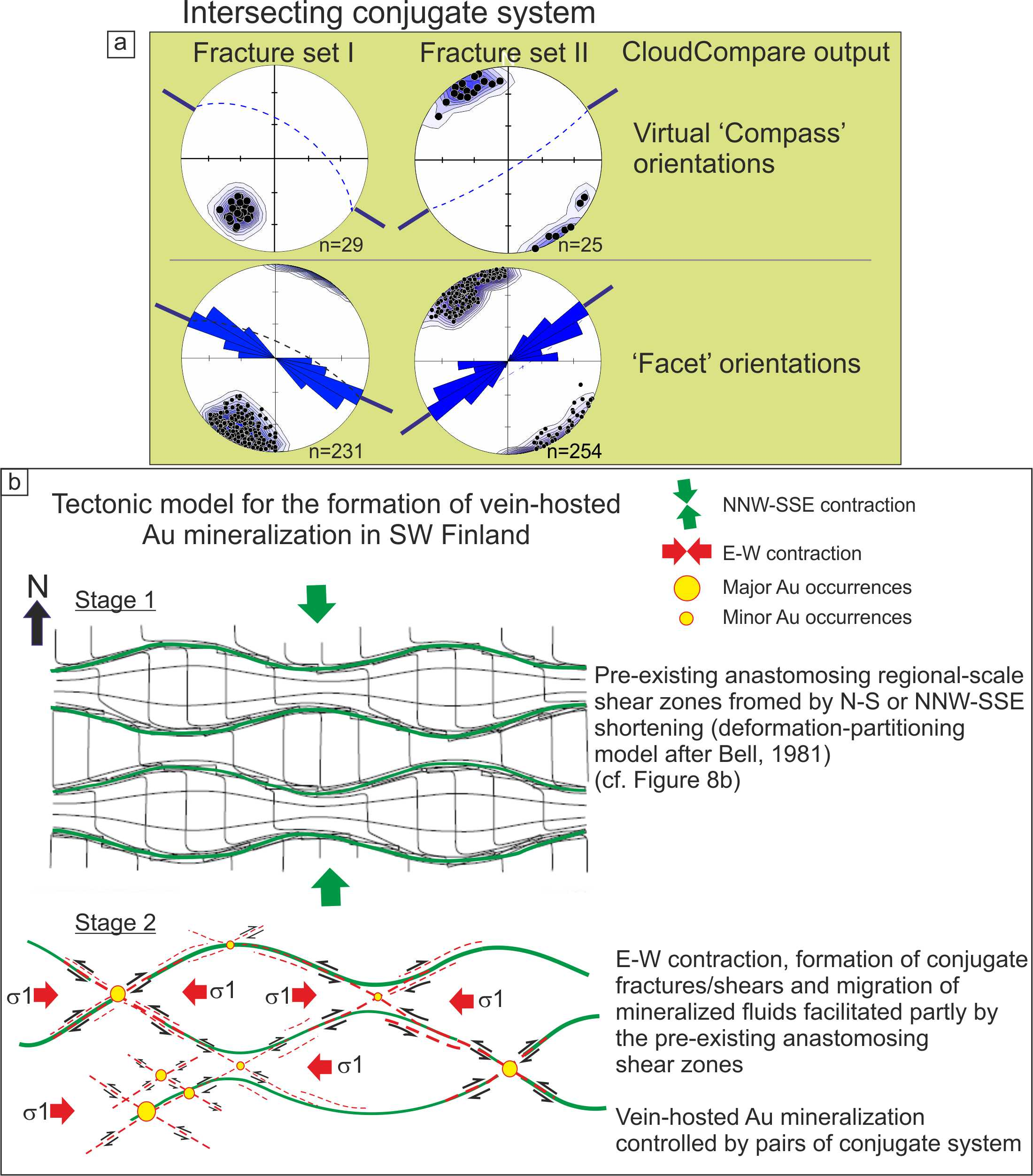
5.2. Tectonic Implications

The Jokisivu gold deposit and other significant gold occurrences in SW Finland show a marked structural control along major pre-existing crustal-scale shear zones [12]. The E-W striking anastomosing geometry of these shear zones reflects strain heterogeneity across different litho-tectonic belts, known as the Tampere schist belt, Pirkanmaa belt, and Häme schist belt (Figure 8b). Based on the conjugate geometry of fracture sets I and II, and the cross-cutting relationships between mineralized shear fractures, we interpret that the regional shear zone network was reactivated during the late-orogenic (D5) phase of E-W contraction. The latter constitutes the waning stage of the Svecofennian orogeny [33]. The shear zones themselves probably formed during the preceding (D4 or pre-D4) phase of NNW-SSE crustal shortening (Figure 9b). Similar structural controls have been proposed also for other late-kinematic orogenic gold bearing settings [45,46]. This tectonic model has important implications for mineral exploration in the region, which we suggest should focus on the identification and precise mapping of crustal-scale shear zones in Paleoproterozoic SE Finland.

6. Conclusions

We have used high-resolution UAV generated 3-D models to study fractures and the associated mineralized quartz veins in the Jokisivu gold mine of SW Finland. The georeferenced 3-D models of inaccessible rock faces of the open-pit wall allow detailed quantitative structural analyses down to the centimeter scale. The approach is independent of the resolution of the target surface due to the full control of the UAV in capturing the multiple images in X, Y (horizontal), and Z (vertical) directions with respect to the Earth’s surface.

The workflow that is presented in this study is based on the combination of well-established equipment and software programs, which allowed for us to decipher the relative kinematic timing of mineralized fractures via the collection of virtual structural data. Three different fracture sets and associated quartz veins have been identified, virtually mapped, and validated. Fracture sets I and II exhibit a conjugate geometry that matches well with the resource model and mine excavation axes of the Jokisivu gold deposit, highlighting the importance of studying the orientation of fracture sets and associated quartz veins.

We have found a significant correlation between the orientations of fracture sets I and II and regional scale anastomosing gold-bearing shear zones, which leads us to propose that the main phases of gold mineralization in SW Finland occurred during late-orogenic reactivation (D5) of this shear zone network around 1.79–1.77 Ga. This tectono-metallogenic model potentially provides a new framework for further exploration strategies in the region.

References

1. Eisenbeiß, H. UAV Photogrammetry. Ph.D. Thesis, ETH Zürich, Zürich, Switzerland, 2009. [Google Scholar]
2. Carrivick, J.; Smith, M.; Quincey, D. Structure from Motion in the Geosciences; Wiley-Blackwell: Hoboken, NJ, USA, 2016; ISBN 9781118895849. [Google Scholar]
3. Westoby, M.J.; Brasington, J.; Glasser, N.F.; Hambrey, M.J.; Reynolds, J.M. “Structure-from-Motion” photogrammetry: A low-cost, effective tool for geoscience applications. Geomorphology 2012, 179, 300–314. [Google Scholar] [CrossRef] [Green Version]
4. Bemis, S.P.; Micklethwaite, S.; Turner, D.; James, M.R.; Akciz, S.; Thiele, S.T.; Bangash, H.A. Ground-based and UAV-Based photogrammetry: A multi-scale, high-resolution mapping tool for structural geology and paleoseismology. J. Struct. Geol. 2014, 69, 163–178. [Google Scholar] [CrossRef]
5. Tavani, S.; Granado, P.; Corradetti, A.; Girundo, M.; Iannace, A.; Arbués, P.; Muñoz, J.A.; Mazzoli, S. Building a virtual outcrop, extracting geological information from it, and sharing the results in Google Earth via OpenPlot and Photoscan: An example from the Khaviz Anticline (Iran). Comput. Geosci. 2014, 63, 44–53. [Google Scholar] [CrossRef]
6. Tong, X.; Liu, X.; Chen, P.; Liu, S.; Luan, K.; Li, L.; Liu, S.; Liu, X.; Xie, H.; Jin, Y.; et al. Integration of UAV-based photogrammetry and terrestrial laser scanning for the three-dimensional mapping and monitoring of open-pit mine areas. Remote Sens. 2015, 7, 6635–6662. [Google Scholar] [CrossRef]
7. Vollgger, S.A.; Cruden, A.R. Mapping folds and fractures in basement and cover rocks using UAV photogrammetry, Cape Liptrap and Cape Paterson, Victoria, Australia. J. Struct. Geol. 2016, 85, 168–187. [Google Scholar] [CrossRef]
8. Riquelme, A.J.; Abellán, A.; Tomás, R.; Jaboyedoff, M. A new approach for semi-automatic rock mass joints recognition from 3D point clouds. Comput. Geosci. 2014, 68, 38–52. [Google Scholar] [CrossRef] [Green Version]
9. Riquelme, A.J.; Tomás, R.; Abellán, A. Characterization of rock slopes through slope mass rating using 3D point clouds. Int. J. Rock Mech. Min. Sci. 2016, 84, 165–176. [Google Scholar] [CrossRef] [Green Version]
10. Cawood, A.J.; Bond, C.E.; Howell, J.A.; Butler, R.W.H.; Totake, Y. LiDAR, UAV or compass-clinometer? Accuracy, coverage and the effects on structural models. J. Struct. Geol. 2017, 98, 67–82. [Google Scholar] [CrossRef] [Green Version]
11. Ojala, J. Gold in the Central Lapland Greenstone Belt; Special Pa; Geological Survey of Finland: Espoo, Finland, 2007; ISBN 9789522170200. [Google Scholar]
12. Eilu, P. Mineral Deposits and Metallogeny of Fennoscandia, 2nd ed.; Geological Survey of Finland: Espoo, Finland, 2012; ISBN 9789522171740. [Google Scholar]
13. Sayab, M.; Suuronen, J.-P.; Molnár, F.; Villanova, J.; Kallonen, A.; O’Brien, H.; Lahtinen, R.; Lehtonen, M. Three-dimensional textural and quantitative analyses of orogenic gold at the nanoscale. Geology 2016, 44. [Google Scholar] [CrossRef]
14. Saalmann, K.; Mänttäri, I.; Peltonen, P.; Whitehouse, M.J.; Grönholm, P.; Talikka, M. Geochronology and structural relationships of mesothermal gold mineralization in the Palaeoproterozoic Jokisivu prospect, southern Finland. Geol. Mag. 2010, 147, 551–569. [Google Scholar] [CrossRef]
15. Ullman, S. The Interpretation of Structure from Motion. Proc. R. Soc. Lond. B Biol. Sci. 1979, 203, 405–426. [Google Scholar] [CrossRef] [PubMed]
16. Lowe, D.G. Distinctive image features from scale-invariant keypoints. Int. J. Comput. Vis. 2004, 60, 91–110. [Google Scholar] [CrossRef]
17. Luhmann, T.; Robson, S.; Kyle, S.; Boehm, J. Close-Range Photogrammetry and 3D Imaging, 2nd ed.; De Gruyter: Berlin, Germany, 2014; ISBN 978-3-11-030278-3. [Google Scholar]
18. Verhoeven, G. Taking computer vision aloft—Archaeological three-dimensional reconstructions from aerial photographs with photoscan. Archaeol. Prospect. 2011, 18, 67–73. [Google Scholar] [CrossRef]
19. Seitz, S.M.; Curless, B.; Diebel, J.; Scharstein, D.; Szeliski, R. A Comparison and Evaluation of Multi-View Stereo Reconstruction Algorithms. In Proceedings of the 2006 IEEE Computer Society Conference on Computer Vision and Pattern Recognition (CVPR’06), New York, NY, USA, 17–22 June 2006; Volume 1, pp. 519–528. [Google Scholar]
20. Bradley, D.; Boubekeur, T.; Heidrich, W. Accurate multi-view reconstruction using robust binocular stereo and surface meshing. In Proceedings of the 2008 IEEE Conference on Computer Vision and Pattern Recognition, Anchorage, AK, USA, 23–28 June 2008; pp. 1–8. [Google Scholar]
21. Snavely, N.; Seitz, S.M.; Szeliski, R. Modeling the world from Internet photo collections. Int. J. Comput. Vis. 2008, 80, 189–210. [Google Scholar] [CrossRef]
22. Triggs, B.; McLauchlan, P.F.; Hartley, R.I.; Fitzgibbon, A.W. Bundle Adjustment—A Modern Synthesis; Springer: Berlin/Heidelberg, Germany, 2000; pp. 298–372. [Google Scholar]
23. Turner, D.; Lucieer, A.; Watson, C. An automated technique for generating georectified mosaics from ultra-high resolution Unmanned Aerial Vehicle (UAV) imagery, based on Structure from Motion (SFM) point clouds. Remote Sens. 2012, 4, 1392–1410. [Google Scholar] [CrossRef]
24. Turner, D.; Lucieer, A.; Wallace, L. Direct georeferencing of ultrahigh-resolution UAV imagery. IEEE Trans. Geosci. Remote Sens. 2014, 52, 2738–2745. [Google Scholar] [CrossRef]
25. James, M.R.; Robson, S. Mitigating systematic error in topographic models derived from UAV and ground-based image networks. Earth Surf. Process. Landf. 2014, 39, 1413–1420. [Google Scholar] [CrossRef] [Green Version]
26. Gonçalves, J.A.; Henriques, R. UAV photogrammetry for topographic monitoring of coastal areas. ISPRS J. Photogramm. Remote Sens. 2015, 104, 101–111. [Google Scholar] [CrossRef]
27. Luukkonen, A. Main Geological Features, Metallogeny and Hydrothermal Alteration Phenomena of Certain Gold and Gold-Tin-Tungsten Prospects in Southern Finland; University of Helsinki: Helsinki, Finland, 1994. [Google Scholar]
28. Thiele, S.T.; Grose, L.; Samsu, A.; Micklethwaite, S.; Vollgger, S.A.; Cruden, A.R. Rapid, semi-automatic fracture and contact mapping for point clouds, images and geophysical data. Solid Earth 2017, 8, 1241–1253. [Google Scholar] [CrossRef] [Green Version]
29. Dewez, T.J.B.; Girardeau-Montaut, D.; Allanic, C.; Rohmer, J. Facets: A cloudcompare plugin to extract geological planes from unstructured 3D point clouds. Int. Arch. Photogramm. Remote Sens. Spat. Inf. Sci. ISPRS Arch. 2016, 41, 799–804. [Google Scholar] [CrossRef]
30. Korsman, K.; Koistinen, T.; Kohonen, J.; Wennerstrom, M.; Ekdahl, E.; Honkamo, M.; Idman, H.; Pekkala, Y. Bedrock Map of Finland 1:1,000,000 Scale; Geological Survey of Finland: Espoo, Finland, 1997. [Google Scholar]
31. Sayab, M.; Suuronen, J.P.; Hölttä, P.; Aerden, D.; Lahtinen, R.; Kallonen, A.P. High-resolution X-ray computed microtomography: A holistic approach to metamorphic fabric analyses. Geology 2015, 43, 55–58. [Google Scholar] [CrossRef] [Green Version]
32. Skyttä, P.; Väisänen, M.; Mänttäri, I. Preservation of Palaeoproterozoic early Svecofennian structures in the Orijärvi area, SW Finland-Evidence for polyphase strain partitioning. Precambrian Res. 2006, 150, 153–172. [Google Scholar] [CrossRef]
33. Lahtinen, R.; Sayab, M.; Karell, F. Near-orthogonal deformation successions in the poly-deformed Paleoproterozoic Martimo belt: Implications for the tectonic evolution of Northern Fennoscandia. Precambrian Res. 2015, 270, 22–38. [Google Scholar] [CrossRef]
34. Bell, T.H. Foliation development—The contribution, geometry and significance of progressive, bulk, inhomogeneous shortening. Tectonophysics 1981, 75, 273–296. [Google Scholar] [CrossRef]
35. Sayab, M.; Khan, M.A. Temporal evolution of surface rupture deduced from coseismic multi-mode secondary fractures: Insights from the October 8, 2005 (Mw 7.6) Kashmir earthquake, NW Himalaya. Tectonophysics 2010, 493, 58–73. [Google Scholar] [CrossRef]
36. Hessami, K.; Koyi, H.A.; Talbot, C.J. The significance of strike slip faulting in basement zagros fold and thrust belt. J. Pet. Geol. 2001, 24, 5–28. [Google Scholar] [CrossRef]
37. Bishop, M.P.; Shroder, J.F. Remote sensing and geomorphometric assessment of topographic complexity and erosion dynamics in the Nanga Parbat massif Remote sensing and geomorphometric assessment of topographic complexity and erosion. Geol. Soc. Lond. Spec. Publ. 2000, 170, 181–200. [Google Scholar] [CrossRef]
38. Sayab, M. Tectonic significance of structural successions preserved within low-strain pods: Implications for thin- to thick-skinned tectonics vs. multiple near-orthogonal folding events in the Palaeo-Mesoproterozoic Mount Isa Inlier (NE Australia). Precambrian Res. 2009, 175, 169–186. [Google Scholar] [CrossRef]
39. Malehmir, A.; Tryggvason, A.; Lickorish, H.; Weihed, P. Regional structural profiles in the western part of the Palaeoproterozoic Skellefte Ore District, northern Sweden. Precambrian Res. 2007, 159, 1–18. [Google Scholar] [CrossRef]
40. Sayab, M.; Miettinen, A.; Aerden, D.; Karell, F. Orthogonal switching of AMS axes during type-2 fold interference: Insights from integrated X-ray computed tomography, AMS and 3D petrography. J. Struct. Geol. 2017, 103. [Google Scholar] [CrossRef]
41. Peterson, D.L.; Brass, J.A.; Smith, W.H.; Langford, G.; Wegener, S.; Dunagan, S.; Hammer, P.; Snook, K. Platform options of free-flying satellites, UAVs or the International Space Station for remote sensing assessment of the littoral zone. Int. J. Remote Sens. 2003. [Google Scholar] [CrossRef]
42. Read, J.; Stacey, P. Guidelines for Open Pit Slope Design; CSIRO Publishing: Clayton, Australia, 2009; ISBN 9780643094697. [Google Scholar]
43. Chen, J.; Li, K.; Chang, K.J.; Sofia, G.; Tarolli, P. Open-pit mining geomorphic feature characterisation. Int. J. Appl. Earth Obs. Geoinf. 2015, 42, 76–86. [Google Scholar] [CrossRef]
44. Lucieer, A.; de Jong, S.M.; Turner, D. Mapping landslide displacements using Structure from Motion (SfM) and image correlation of multi-temporal UAV photography. Prog. Phys. Geogr. 2014, 38, 97–116. [Google Scholar] [CrossRef]
45. Groves, D.I.; Goldfarb, R.J.; Knox-Robinson, C.M.; Ojala, J.; Gardoll, S.; Yun, G.Y.; Holyland, P. Late-kinematic timing of orogenic gold deposits and significance for computer-based exploration techniques with emphasis on the Yilgarn Block, Western Australia. Ore Geol. Rev. 2000, 17, 1–38. [Google Scholar] [CrossRef]
46. Goldfarb, R.J.; Baker, T.; Dubé, B.; Groves, D.I.; Hart, C.J.R.; Gosselin, P. Distribution, Character, and Genesis of Gold Deposits in Metamorphic Terranes. Soc. Econ. Geol. 2005, 100, 407–450. [Google Scholar] [CrossRef]
Figure 1. (a) Front view of the Phantom 3 Professional. (bd) Showing different camera orientations in horizontal, oblique and vertical positions. (e) Photo showing measurement of a ground control point with the Topcon HiPer® receiver with FC-200 field collector.
Remotesensing 10 01296 g001
Figure 2. Workflow adopted in this study (right side). Explanation of each step is summarized on the (left side).
Remotesensing 10 01296 g002
Figure 3. Steps involved for three-dimensional (3-D) model generation of the Kujankallio open pit and the western extension using SfM. (a) Photo alignment in a reference mode. The blue squares with nadir (center) lines represent camera positions and orientations automatically detected by the PhotoScan from the SfM process. Light blue squares show oblique images. 158 georeferenced images were taken at an altitude of ~79 m. 11 ground control points (GCPs) were deployed and incorporated their locations during the Photoscan workflow. (b) Digital elevation model (DEM) of the open pit showing elevation gradient from blue to red. Blue flags indicate location of GCPs. (c) Orthorectified image showing location of the surface profile sections and length of the warehouse. Thick yellow line showing the location of the northern face used for virtual quantitative structural analysis. Coordinates are in ETRS89/TM35FIN (3067). (d) Two profile sections (AB and CD) highlighting the surface geometry of the open pit.
Remotesensing 10 01296 g003
Figure 4. (a) High-resolution (1.4 cm/pixel) textured photogrammetric 3-D model of selected portions of the northern face (see Figure 3c for location). 69 georeferenced images were taken using the Phantom 3 Professional with the camera axis kept horizontal. (b) Three representative areas outlined with rectangular boxes (W, X, Y) where ‘virtual’ structural measurements were collected. (c,d) Close ups of area W viewed from different angles showing fracture set I and III and associated quartz veins 1 and 2. Vein set 2 is parallel to fracture set III. Fracture set III cuts fracture set I. (e) Area X exposing fracture set I and quartz vein sets 1 and 2. (f) Fracture sets I and II in Area Y.
Remotesensing 10 01296 g004
Figure 5. (a) Virtual structural data obtained from the 3-D model using the ‘Compass’ tool of ClouldCompare. (b) Orientations for fracture set I exhibit a prominent NW-SE strike and moderate dip to the NE. (c) Stereoplot of set II fractures striking NE-SW and very steeply dipping SE. (d) Fracture set III is NNW-SSE striking and steeply dipping towards the SW.
Remotesensing 10 01296 g005
Figure 6. Comparison of virtual ‘Compass’ measurements and field data. (a,b) Fractures labeled 1, 2, and 3 exposed at the bottom of the pit wall (highlighted in red boxes) that were used to check the orientations obtained with the ‘Compass’ tool. All of the fractures belong to Set I. Inset (green box) in ‘a’ shows length of the 50 m scale bar measured in the Photoscan. (c) Orientations measured in the field and virtually with the ‘Compass’ plugin showing a very close match. (d) Fracture belonging to set II and III measured on the southern face of the open pit with a similar orientation as those measured with the ‘Compass’ plugin from the northern face (cf. Figure 5c,d).
Remotesensing 10 01296 g006
Figure 7. Fracture planes and their orientations extracted using the ‘Facet’ plugin with an angular step at 5°. Different colors represent dip direction in all sub figures. Results were further analyzed in ArcMap to categorize dip directions. (a) Fracture set I and (b) ArcMap analysis showing facets in two distinct colors based on dip direction. ‘Facet’ data is plotted in a rose diagram and associated poles of fracture planes. The dominant strike of the fractures is NW-SE. (c) ‘Facet’ analysis of fracture set II trending NE-SW and (d) corresponding ArcMap plot. (e) Orientation of fracture set III calculated using ‘Facets’ and (f) ArcMap analysis. See text for further explanation. Colors palettes refer to dip directions in (d,f).
Remotesensing 10 01296 g007aRemotesensing 10 01296 g007b
Figure 8. (a) Surface resource model of the open-pit mine showing a good match with the strikes of fracture sets I and II. (b) Map showing the regional pattern of major shear zones (after [27,30]) and locations of various gold deposits and prospects in SW Finland: (1) Kedonojankulma, (2) Kivenkorva W, (3) Kivenkorva E, (4) Kokkojoki, 5) Riukka, (6) Satulinmäki, (7) Sukula, (8) Uunimäki, (9) Jokisivu, (10) Korvenmaa, (11) Palokallio, (12) Ritakallio, (13) Liesjärvi, (14) Hopeavuori, (15) Kaapelinkulma. Tectonic domains: TB, Tampere schist belt; PB, Pirkanmaa belt; HB, Häme schist belt. Inset shows mean orientations of fracture sets I, II and III.
Remotesensing 10 01296 g008
Figure 9. (a) Orientation data for fracture sets I and II. Virtual outcrop analysis allows for interpretation of fracture sets I and II as a conjugate pair. (b) Tectonic model showing pre-existing anastomosing shear zones formed syn- or pre-D4 (NNW-SSE contraction), which were later reactivated with the formation of new conjugate shears during E-W tectonic shortening (D5). Intersecting areas could be potential sites of gold occurrences as seen in the case of Jokisivu gold mine, Satulinmäki and other gold prospects.
Remotesensing 10 01296 g009