Regional Patterns and Asynchronous Onset of Ice-Wedge Degradation since the Mid-20th Century in Arctic Alaska

 , ,
, ,
Abstract
:
1. Introduction
2. Materials and Methods
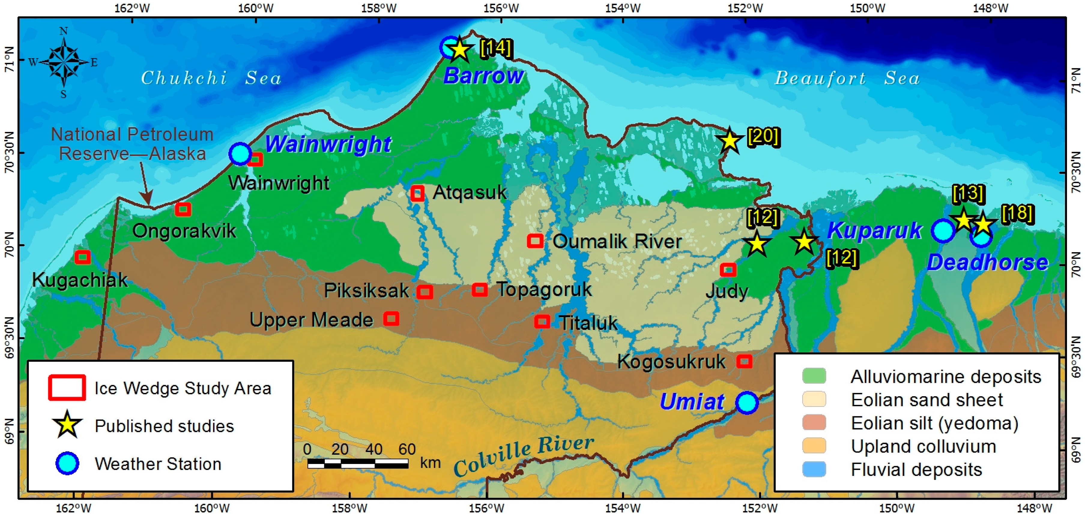
2.1. Study Area
2.2. Data Sources
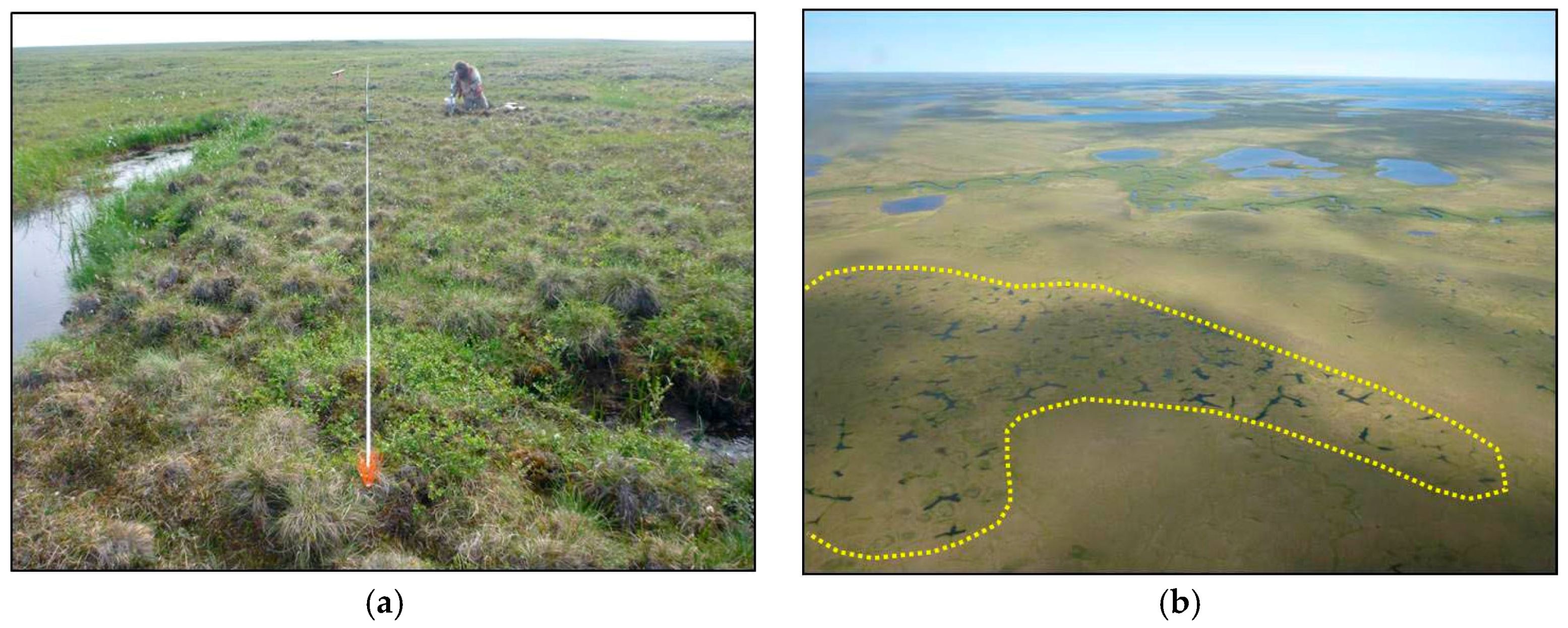
2.3. Field Observations and Terrain Mapping
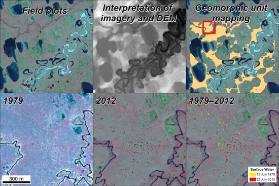
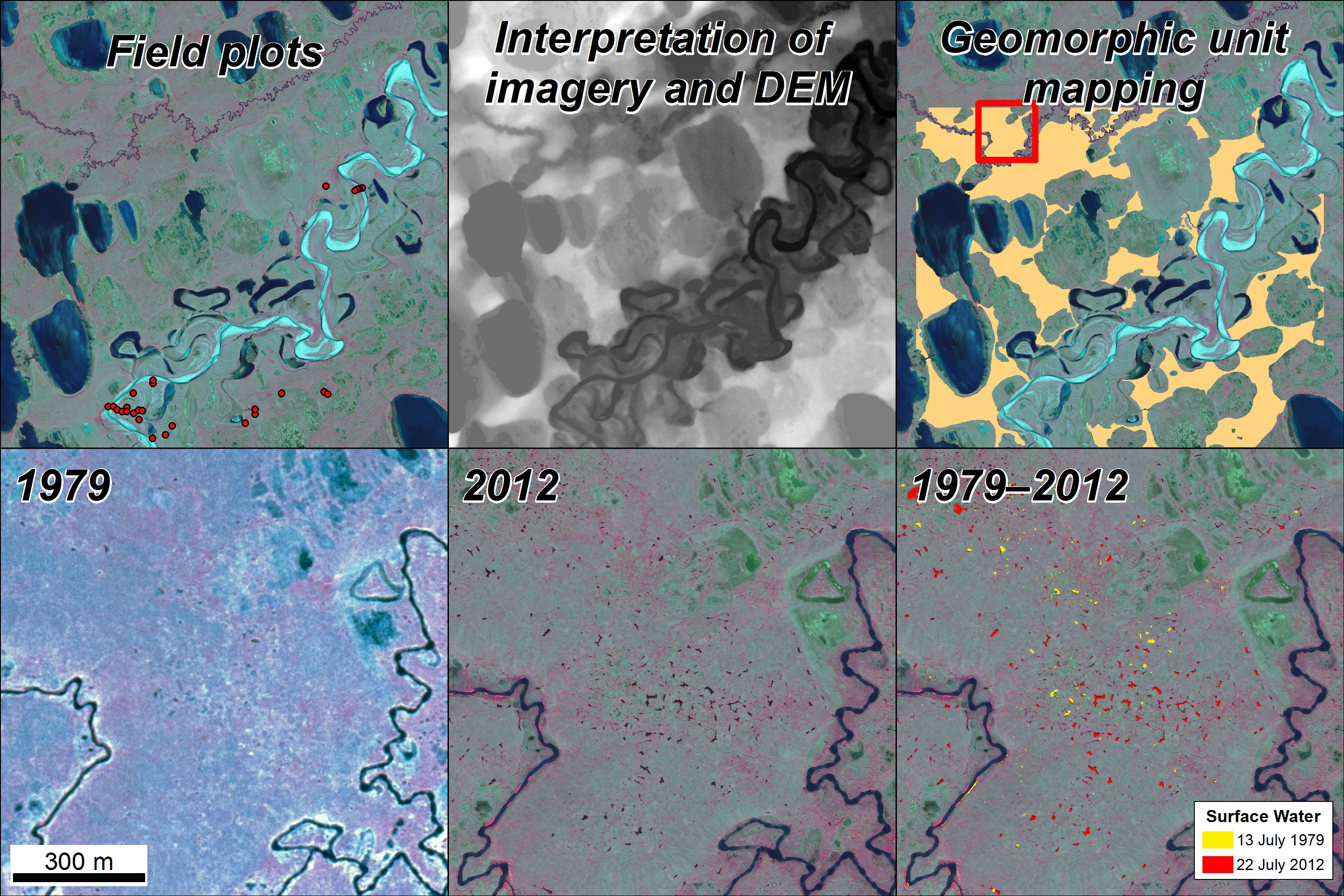
2.4. Surface Water Mapping
3. Results
3.1. Field Observations and Terrain Mapping
3.2. Surface Water Mapping
4. Discussion
4.1. Mechanisms for Asynchronous Onset
4.2. Sources of Uncertainty
4.3. Implications for North Slope Ecosystems
5. Conclusions
Supplementary Materials
Author Contributions
Funding
Acknowledgments
Conflicts of Interest
References
- Washburn, A.L. Geocryology: A Survey of Periglacial Processes and Environments; John Wiley & Sons, Inc.: Hoboken, NJ, USA, 1980. [Google Scholar]
- French, H.M. The Periglacial Environment; John Wiley & Sons, Ltd: Chichester, UK, 2007. [Google Scholar]
- De Koven Leffingwell, E. The Canning River Region, Northern Alaska; Government Printing Office: Washington, DC, USA, 1919.
- Lachenbruch, A.H. Mechanics of Thermal Contraction Cracks and Ice-Wedge Polygons in Permafrost; The Waverly Press: Baltimore, MD, USA, 1962. [Google Scholar]
- Romanovskii, N. Formation of Ice Wedges—Polygonal Patterns; Nauka: Novosibirsk, Russia, 1977. [Google Scholar]
- Jorgenson, M.T.; Shur, Y. Evolution of lakes and basins in northern Alaska and discussion of the thaw lake cycle. J. Geophys. Res. 2007, 112. [Google Scholar] [CrossRef] [Green Version]
- Schirrmeister, L.; Froese, D.; Tumskoy, V.; Wetterich, S. Yedoma: Late Pleistocene ice-rich syngenetic permafrost of Beringia. In Encyclopedia of Quaternary Science, 2nd ed.; Elias, S.A., Mock, C.J., Eds.; Elsevier: Amsterdam, The Netherlands, 2012; pp. 542–552. [Google Scholar]
- Gallant, A.L.; Binnian, E.F.; Omernik, J.M.; Shasby, M.B. Ecoregions of Alaska; United States Government Printing Office: Washington, DC, USA, 1995.
- Kanevskiy, M.; Shur, Y.; Fortier, D.; Jorgenson, M.T.; Stephani, E. Cryostratigraphy of late Pleistocene syngenetic permafrost (yedoma) in northern Alaska, Itkillik River exposure. Quat. Res. 2011, 75, 584–596. [Google Scholar] [CrossRef]
- Liljedahl, A.K.; Hinzman, L.D.; Schulla, J. Ice-wedge polygon type controls low-gradient watershed-scale hydrology. In Proceedings of the Tenth International Conference on Permafrost, Salekhard, Russia, 25–29 June 2012; pp. 231–236. [Google Scholar]
- Anderson, B.A.; Cooper, B.A. Distribution and Abundance of Spectacled Eiders in the Kuparuk and Milne Point Oilfields, Alaska, 1993; Alaska Biological Research, Inc.: Fairbanks, AK, USA, 1994. [Google Scholar]
- Jorgenson, M.T.; Shur, Y.L.; Pullman, E.R. Abrupt increase in permafrost degradation in Arctic Alaska. Geophys. Res. Lett. 2006, 33. [Google Scholar] [CrossRef] [Green Version]
- Raynolds, M.K.; Walker, D.A.; Ambrosius, K.J.; Brown, J.; Everett, K.R.; Kanevskiy, M.; Kofinas, G.P.; Romanovsky, V.E.; Shur, Y.; Webber, P.J. Cumulative geoecological effects of 62 years of infrastructure and climate change in ice-rich permafrost landscapes, Prudhoe Bay Oilfield, Alaska. Glob. Chang. Biol. 2014, 20, 1211–1224. [Google Scholar] [CrossRef] [PubMed]
- Liljedahl, A.K.; Boike, J.; Daanen, R.P.; Fedorov, A.N.; Frost, G.V.; Grosse, G.; Hinzman, L.D.; Iijma, Y.; Jorgenson, J.C.; Matveyeva, N.; et al. Pan-Arctic ice-wedge degradation in warming permafrost and its influence on tundra hydrology. Nat. Geosci. 2016, 9, 312–318. [Google Scholar] [CrossRef]
- Necsoiu, M.; Dinwiddie, C.L.; Walter, G.R.; Larsen, A.; Stothoff, S.A. Multi-temporal image analysis of historical aerial photographs and recent satellite imagery reveals evolution of water body surface area and polygonal terrain morphology in Kobuk Valley National Park, Alaska. Environ. Res. Lett. 2013, 8. [Google Scholar] [CrossRef]
- Kokelj, S.V.; Lantz, T.C.; Wolfe, S.A.; Kanigan, J.C.; Morse, P.D.; Coutts, R.; Molina-Giraldo, N.; Burn, C.R. Distribution and activity of ice wedges across the forest-tundra transition, western Arctic Canada: Ice wedges across tree line. J. Geophys. Res. Earth Surf. 2014, 119, 2032–2047. [Google Scholar] [CrossRef]
- Wolter, J.; Lantuit, H.; Fritz, M.; Macias-Fauria, M.; Myers-Smith, I.; Herzschuh, U. Vegetation composition and shrub extent on the Yukon coast, Canada, are strongly linked to ice-wedge polygon degradation. Polar Res. 2016, 35. [Google Scholar] [CrossRef] [Green Version]
- Jorgenson, M.T.; Kanevskiy, M.; Shur, Y.; Moskalenko, N.; Brown, D.R.N.; Wickland, K.; Striegl, R.; Koch, J. Role of ground ice dynamics and ecological feedbacks in recent ice wedge degradation and stabilization. J. Geophys. Res. Earth Surf. 2015, 120. [Google Scholar] [CrossRef]
- Kanevskiy, M.; Shur, Y.; Jorgenson, T.; Brown, D.R.N.; Moskalenko, N.; Brown, J.; Walker, D.A.; Raynolds, M.K.; Buchhorn, M. Degradation and stabilization of ice wedges: Implications for assessing risk of thermokarst in northern Alaska. Geomorphology 2017, 297, 20–42. [Google Scholar] [CrossRef]
- Tape, K.D.; Flint, P.L.; Meixell, B.W.; Gaglioti, B.V. Inundation, sedimentation, and subsidence creates goose habitat along the Arctic coast of Alaska. Environ. Res. Lett. 2013, 8. [Google Scholar] [CrossRef]
- Jones, B.M.; Grosse, G.; Arp, C.D.; Miller, E.; Liu, L.; Hayes, D.J.; Larsen, C.F. Recent Arctic tundra fire initiates widespread thermokarst development. Sci. Rep. 2015, 5. [Google Scholar] [CrossRef] [PubMed] [Green Version]
- Carter, L.D. A Pleistocene sand sea on the Alaskan Arctic coastal plain. Science 1981, 211, 381–383. [Google Scholar] [CrossRef] [PubMed]
- Williams, J.R. Engineering-Geologic Maps of Northern Alaska, Wainwright Quadrangle; U.S. Geological Survey: Menlo Park, CA, USA, 1983.
- Haugen, R.K.; Brown, J. Coastal-inland distributions of summer air temperature and precipitation in northern Alaska. Arct. Alp. Res. 1980, 12, 403–412. [Google Scholar] [CrossRef]
- Circumpolar arctic vegetation map (1:7,500,000 scale), Conservation of Arctic Flora and Fauna (CAFF) Map No. 1. 2003. Available online: https://www.geobotany.uaf.edu/cavm/ (accessed on 3 June 2018).
- Jorgenson, M.T.; Grunblatt, J. Landscape-Level Ecological Mapping of Northern Alaska and Field Site Photography; U.S. Fish and Wildlife Service: Fairbanks, AK, USA, 2013.
- Jorgenson, M.T.; Roth, J.E.; Miller, P.F.; Macander, M.J.; Duffy, M.S.; Wells, A.F.; Frost, G.V.; Pullman, E.R. An Ecological Land Survey and Landcover Map of the Arctic Network; U.S. Department of the Interior: Fort Collins, CO, USA, 2009.
- Kreig, R.A.; Reger, R.D. Air-Photo Analysis and Summary of Land-Form Soil Properties Along the Route of the Trans-Alaska Pipeline System; Alaska Division of Geological and Geophysical Surveys: Fairbanks, AK, USA, 1982.
- Viereck, L.A.; Dyrness, C.T.; Batten, A.R.; Wenzlick, K.J. The Alaska Vegetation Classification; U.S. Department of Agriculture, Forest Service, Pacific Northwest Research Station: Portland, OR, USA, 1992.
- Burn, C.R.; Zhang, Y. Permafrost and climate change at Herschel Island (Qikiqtaruq), Yukon Territory, Canada. J. Geophys. Res. Earth Surf. 2009, 114. [Google Scholar] [CrossRef] [Green Version]
- Johannessen, O.M.; Bengtsson, L.; Miles, M.W.; Kuzmina, S.I.; Semenov, V.A.; Alekseev, G.V.; Nagurnyi, A.P.; Zakharov, V.F.; Bobylev, L.P.; Pettersson, L.H.; et al. Arctic climate change: Observed and modelled temperature and sea-ice variability. Tellus A Dyn. Meteorol. Oceanogr. 2004, 56, 328–341. [Google Scholar] [CrossRef] [Green Version]
- Harris, I.; Jones, P.D.; Osborn, T.J.; Lister, D.H. Updated high-resolution grids of monthly climatic observations—The CRU TS3.10 Dataset. Int. J. Climatol. 2013, 34, 623–642. [Google Scholar] [CrossRef] [Green Version]
- Mantua, N.J.; Hare, S.R.; Zhang, Y.; Wallace, J.M.; Francis, R.C.A. Pacific interdecadal climate oscillation with impacts on salmon production. Bull. Am. Meteorol. Soc. 1997, 78, 1069–1079. [Google Scholar] [CrossRef]
- Cai, L.; Alexeev, V.A.; Arp, C.D.; Jones, B.M.; Liljedahl, A.K.; Gädeke, A. The Polar WRF downscaled historical and projected twenty-first century climate for the coast and foothills of Arctic Alaska. Front. Earth Sci. 2018, 5. [Google Scholar] [CrossRef]
- Shur, Y.L.; Jorgenson, M.T. Patterns of permafrost formation and degradation in relation to climate and ecosystems. Permafr. Periglac. Process. 2007, 18, 7–19. [Google Scholar] [CrossRef]
- Shur, Y.; Hinkel, K.M.; Nelson, F.E. The transient layer: Implications for geocryology and climate-change science. Permafr. Periglac. Process. 2005, 16, 5–17. [Google Scholar] [CrossRef]
- Farquharson, L.M.; Mann, D.H.; Grosse, G.; Jones, B.M.; Romanovsky, V.E. Spatial distribution of thermokarst terrain in Arctic Alaska. Geomorphology 2016, 273, 116–133. [Google Scholar] [CrossRef] [Green Version]
- Jorgenson, M.T.; Grosse, G. Remote sensing of landscape change in permafrost regions. Permafr. Periglac. Process. 2016, 27, 324–338. [Google Scholar] [CrossRef]
- Bartsch, A.; Höfler, A.; Kroisleitner, C.; Trofaier, A. Land cover mapping in northern high latitude permafrost regions with satellite data: Achievements and remaining challenges. Remote Sens. 2016, 8, 979. [Google Scholar] [CrossRef]
- Liljedahl, A.K.; Hinzman, L.D.; Harazono, Y.; Zona, D.; Tweedie, C.E.; Hollister, R.D.; Engstrom, R.; Oechel, W.C. Nonlinear controls on evapotranspiration in arctic coastal wetlands. Biogeosciences 2011, 8, 3375–3389. [Google Scholar] [CrossRef] [Green Version]
- Koch, J.C. Lateral and subsurface flows impact arctic coastal plain lake water budgets. Hydrol. Process. 2016, 30, 3918–3931. [Google Scholar] [CrossRef]
- Liljedahl, A.K.; Hinzman, L.D.; Kane, D.L.; Oechel, W.C.; Tweedie, C.E.; Zona, D. Tundra water budget and implications of precipitation underestimation. Water Resour. Res. 2017, 53, 6472–6486. [Google Scholar] [CrossRef] [PubMed] [Green Version]
- Koch, J.C.; Jorgenson, M.T.; Wickland, K.P.; Kanevskiy, M.; Striegl, R.G. Ice wedge degradation and stabilization impacts water budgets and nutrient cycling in Arctic thaw ponds. J. Geophys. Res. Biogeosci. 2018. [Google Scholar] [CrossRef]
- Macander, M.J.; Swingley, C.S.; Joly, K.; Raynolds, M.K. Landsat-based snow persistence map for northwest Alaska. Remote Sens. Environ. 2015, 163, 23–31. [Google Scholar] [CrossRef]
- Günther, F.; Overduin, P.P.; Sandakov, A.V.; Grosse, G.; Grigoriev, M.N. Short-and long-term thermo-erosion of ice-rich permafrost coasts in the Laptev Sea region. Biogeosciences 2013, 10, 4297–4318. [Google Scholar] [CrossRef] [Green Version]
- Jones, B.M.; Stoker, J.M.; Gibbs, A.E.; Grosse, G.; Romanovsky, V.E.; Douglas, T.A.; Kinsman, N.E.M.; Richmond, B.M. Quantifying landscape change in an arctic coastal lowland using repeat airborne LiDAR. Environ. Res. Lett. 2013, 8. [Google Scholar] [CrossRef]
- Whitley, M.A.; Frost, G.V.; Jorgenson, M.T.; Macander, M.J.; Maio, C.V.; Winder, S.G. Assessment of LiDAR and spectral techniques for high-resolution mapping of sporadic permafrost on the Yukon-Kuskokwim Delta, Alaska. Remote Sens. 2018, 10, 258. [Google Scholar] [CrossRef]
- Lara, M.J.; Nitze, I.; Grosse, G.; Martin, P.; McGuire, A.D. Reduced arctic tundra productivity linked with landform and climate change interactions. Sci. Rep. 2018, 8. [Google Scholar] [CrossRef] [PubMed]


| Station 1 | Mean Temperature (°C) | Mean Precipitation (mm) | ||
|---|---|---|---|---|
| Annual | Summer | Winter | ||
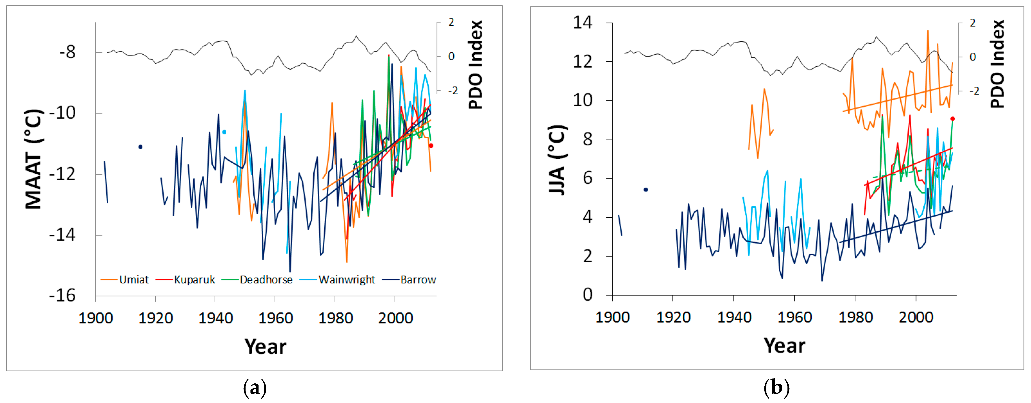
| Wainwright | −9.8 | +5.7 | −22.2 | 98.6 |
| Barrow | −11.4 | +3.5 | −23.1 | 116.9 |
| Umiat | −11.4 | +10.0 | −27.0 | 70.0 |
| Kuparuk | −11.1 | +6.6 | −24.9 | 101.6 |
| Deadhorse | −11.1 | +6.3 | −24.7 | 101.4 |
| Study Area | Region | Lat (°N) | Long (°W) | Period | ||
|---|---|---|---|---|---|---|
| 1950 | 1982 | 2012 1 | ||||
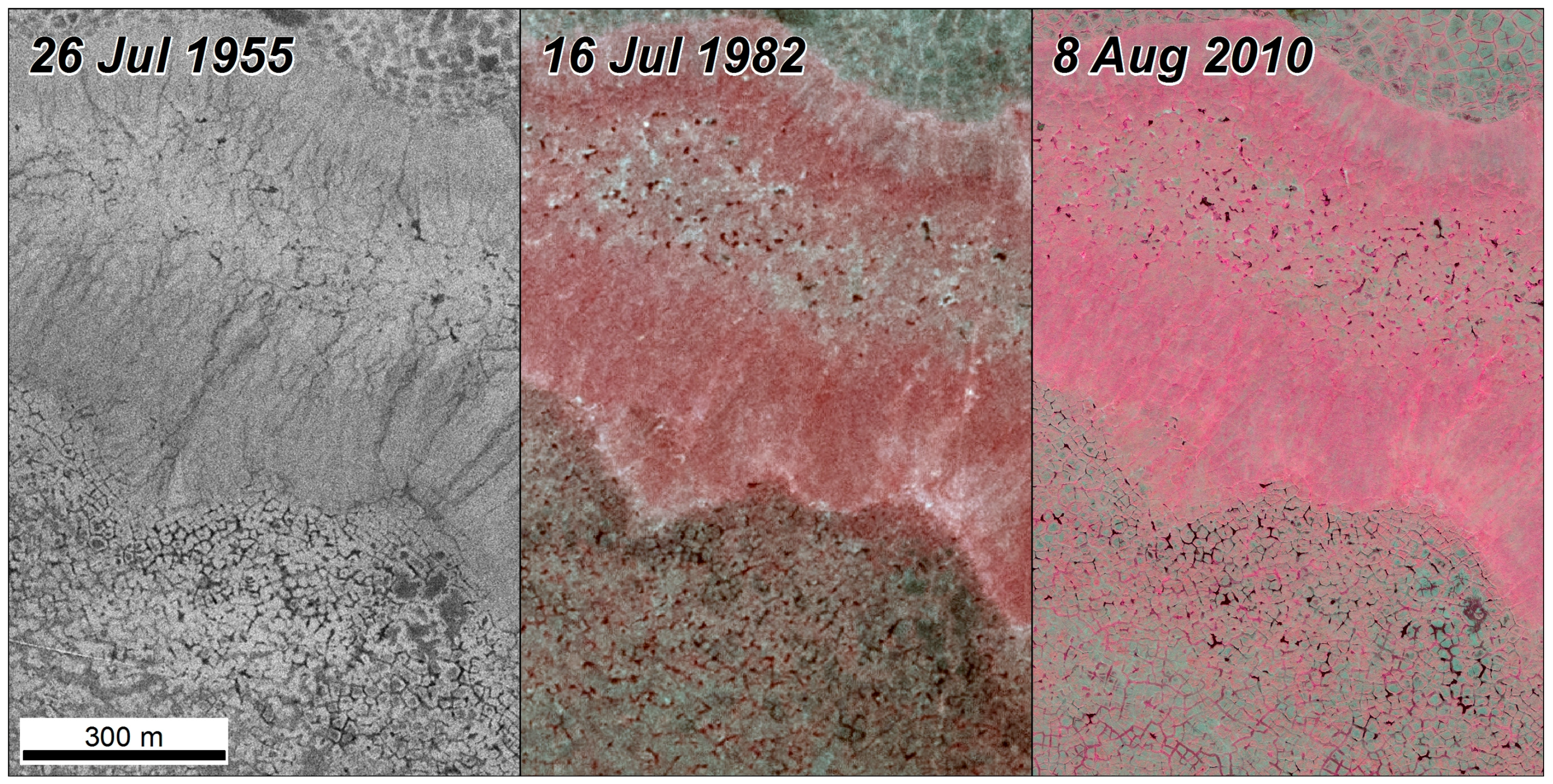
| Kugachiak | Chukchi coastal plain | 70.0 | 162.3 | 26 Jul. 1955 | 16 Jul. 1982 | 8 Aug. 2010 (GE1) |
| Ongorakvik | Chukchi coastal plain | 70.3 | 160.9 | 16 Jul. 1949 | 2 Aug. 1985 | 5 Jul. 2012 (WV2) |
| Wainwright | Chukchi coastal plain | 70.6 | 159.8 | 1 Jul. 1949 | 18 Jul. 1982 | 8 Jul. 2012 (WV2) |
| U. Meade | Arctic foothills | 69.8 | 157.5 | 12 Jul. 1949 | 16 Jul. 1982 | 19 Jul. 2009 (GE1) |
| Atqasuk | Beaufort coastal plain | 70.5 | 157.2 | 25 Jul. 1955 | 2 Aug. 1985 | 22 Jul. 2012 (GE1) |
| Piksiksak | Arctic foothills | 70.0 | 157.0 | 23 Jul. 1955 | 16 Jul. 1982 | 22 Jul. 2012 (GE1) |
| Topagoruk | Arctic foothills | 70.0 | 156.2 | 23 Jul. 1955 | 16 Jul. 1982 | 9 Jul. 2010 (GE1) |
| Oumalik R. | Beaufort coastal plain | 70.3 | 155.4 | 25 Jul. 1955 | 16 Jul. 1982 | 15 Jul. 2009 (GE1) |
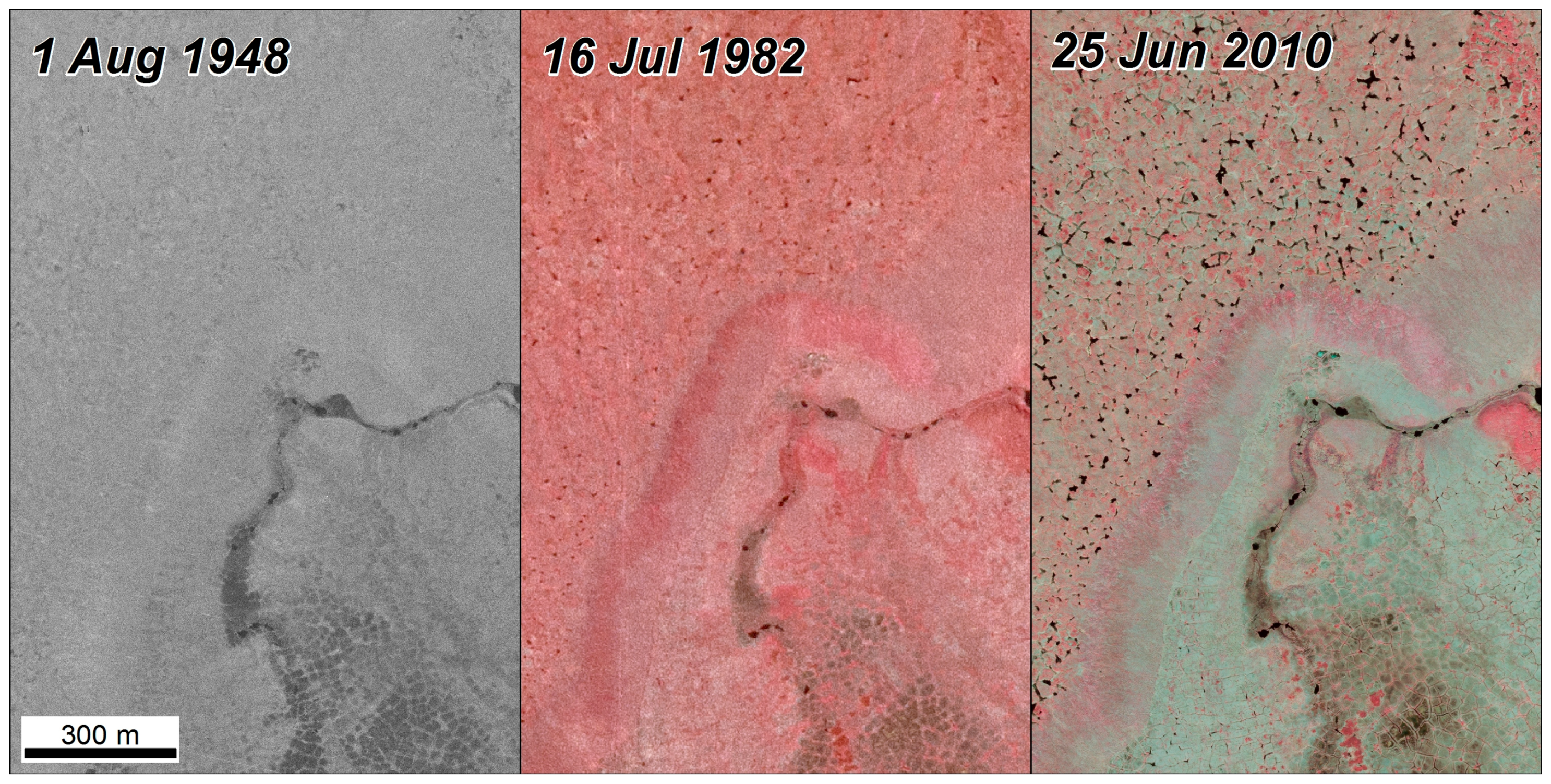
| Titaluk | Arctic foothills | 69.8 | 155.2 | 1 Aug. 1948 | 16 Jul. 1982 | 25 Jun. 2010 (WV2) |
| Judy Creek | Beaufort coastal plain | 70.1 | 152.4 | 24 Jul. 1955 | 13 Jul. 1979 | 22 Jul. 2012 (GE1) |
| Kogosukruk | Arctic foothills | 69.6 | 152.2 | 23 Jul. 1955 | 1 Aug. 1977 | 22 Aug. 2011 (WV2) |
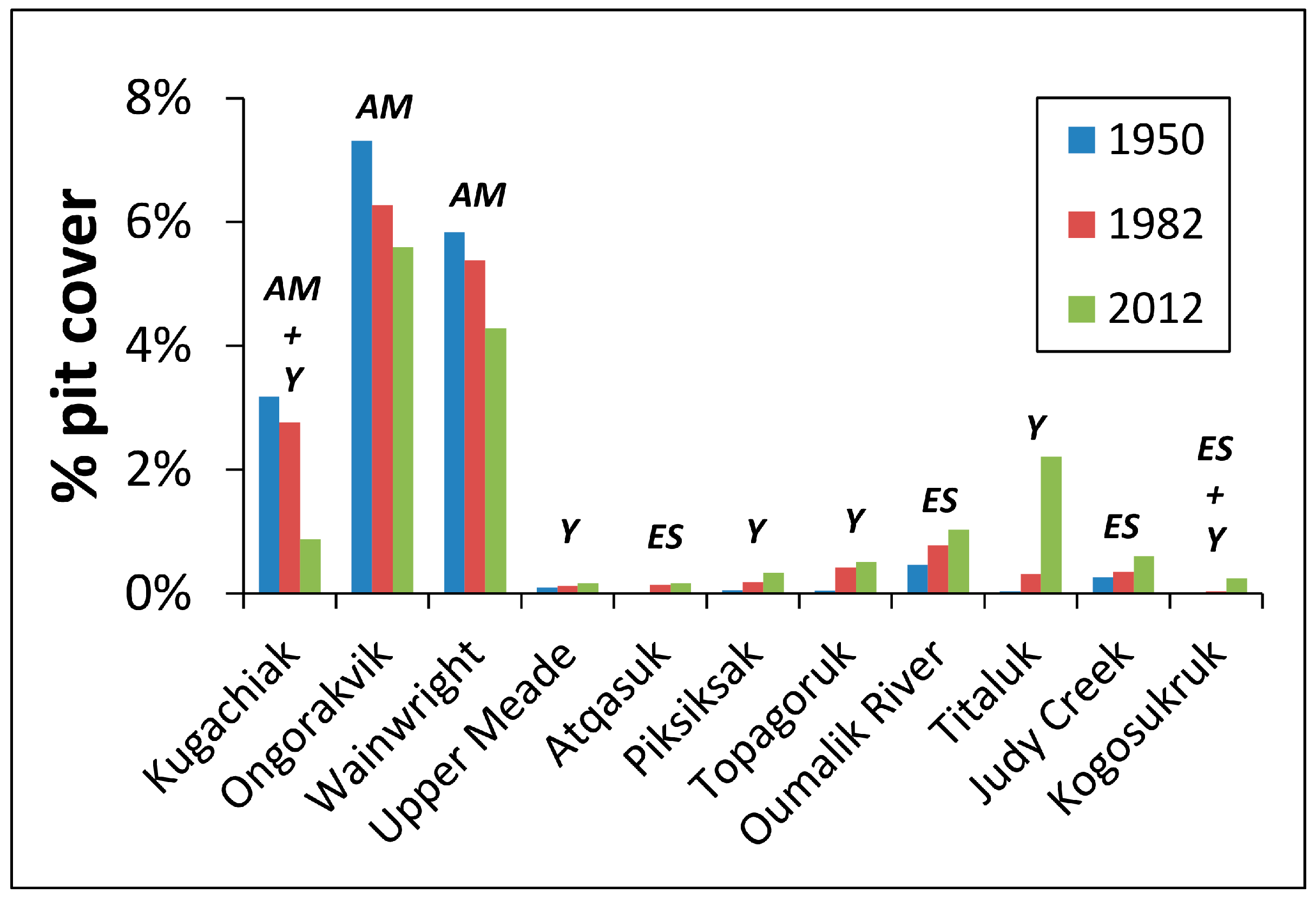
| Study Area | Geomorphic Unit (s) | Residual Upland | Δ Pit Extent (c. 1950–2012) | ||
|---|---|---|---|---|---|
| Area (ha) | % | Area (ha) | % | ||
| Kugachiak | alluvial-marine, yedoma | 1723.3 | 53.9% | −39.7 | −72.5% |
| Ongorakvik | alluvial-marine | 1477.8 | 84.0% | −25.4 | −23.5% |
| Wainwright | alluvial-marine | 750.6 | 47.6% | −11.7 | −26.7% |
| Upper Meade | yedoma | 1200.1 | 73.7% | 0.9 | 74.8% |
| Atqasuk | eolian sand | 1412.0 | 31.7% | 1.9 | 7692.9% |
| Piksiksak | yedoma | 1550.4 | 43.4% | 4.4 | 561.9% |
| Topagoruk | yedoma | 2824.9 | 63.3% | 13.2 | 1080.6% |
| Oumalik River | eolian sand | 941.0 | 55.8% | 5.3 | 122.4% |
| Titaluk | yedoma | 507.4 | 17.8% | 11.0 | 6092.6% |
| Judy Creek | eolian sand | 1059.0 | 23.7% | 3.6 | 130.3% |
| Kogosukruk | eolian sand, yedoma | 2489.7 | 55.8% | 5.5 | 1194.3% |
© 2018 by the authors. Licensee MDPI, Basel, Switzerland. This article is an open access article distributed under the terms and conditions of the Creative Commons Attribution (CC BY) license (http://creativecommons.org/licenses/by/4.0/).
Share and Cite
Frost, G.V.; Christopherson, T.; Jorgenson, M.T.; Liljedahl, A.K.; Macander, M.J.; Walker, D.A.; Wells, A.F. Regional Patterns and Asynchronous Onset of Ice-Wedge Degradation since the Mid-20th Century in Arctic Alaska. Remote Sens. 2018, 10, 1312. https://doi.org/10.3390/rs10081312
Frost GV, Christopherson T, Jorgenson MT, Liljedahl AK, Macander MJ, Walker DA, Wells AF. Regional Patterns and Asynchronous Onset of Ice-Wedge Degradation since the Mid-20th Century in Arctic Alaska. Remote Sensing. 2018; 10(8):1312. https://doi.org/10.3390/rs10081312
Chicago/Turabian StyleFrost, Gerald V., Tracy Christopherson, M. Torre Jorgenson, Anna K. Liljedahl, Matthew J. Macander, Donald A. Walker, and Aaron F. Wells. 2018. "Regional Patterns and Asynchronous Onset of Ice-Wedge Degradation since the Mid-20th Century in Arctic Alaska" Remote Sensing 10, no. 8: 1312. https://doi.org/10.3390/rs10081312