Land Surface Temperature and Urban Density: Multiyear Modeling and Relationship Analysis Using MODIS and Landsat Data


1
Department of Engineering, University of Perugia, via Duranti 93, 06125 Perugia, Italy
2
Department of Computer Science, Khon Kaen University, Khon Kaen 40002, Thailand
*
Author to whom correspondence should be addressed.
Remote Sens. 2018, 10(9), 1471; https://doi.org/10.3390/rs10091471
Submission received: 28 July 2018
/
Revised: 5 September 2018
/
Accepted: 12 September 2018
/
Published: 14 September 2018
(This article belongs to the Special Issue Applications of Land Surface Temperature and its Combination with other Satellite Land Products)
Abstract
:This work aims to model and relate the urban density and land surface temperature (LST) by a straightforward and efficient approach. Although the urban density-LST relation is widely addressed in literature, this study allows for its modeling and parameterization in an accurate way, providing a further scientific support for the city planning policy. The urban density and the LST analysis is carried out in the Bangkok area for the years 2004, 2008, 2012, and 2016; in this time interval, the city exhibited an evident urban expansion. Firstly, by using land cover maps obtained from Landsat reflective observations, the urban land density growth across the years studied is evaluated by applying a ring-based approach, a method employed in urban theory, providing urban density curves as a function of the distance from the city center. For each year, the urban density curve is well modeled by an inverse S-shape function, the parameters of which highlight an urban sprawl over the years studied and an outskirt growth in recent years. Then, employing 237 MODIS LST images, the night-time and daytime mean LST patterns for each year were processed applying the same ring-based analysis, obtaining LST trends versus distance. Albeit the mean LST decreases away from the city core, the daytime and night-time trends are different in both shape and values. The daytime LST exhibits a trend also modeled by an inverse S-shape function, whereas the night-time one is modeled by a quadratic function. Finally, the urban density-LST relationship is inferred across the years: For daytime, the relation is quadratic with a coefficient of determination r2 around 0.98–0.99, whereas for night-time the relation is linear with r2 of the order of 0.95–0.96. The proposed approach allows for reliable modeling and to straightforwardly infer a very accurate urban density-LST relationship.

1. Introduction
The rapid urbanization process plays a key role in the heating phenomenon known as urban heat island (UHI) [1], involving both air and surface temperatures in different ways [2]. The UHI has effects on human comfort, air pollution, energy management, urban planning policy, and climate changes [3,4,5,6,7]. In fact, land surface temperature (LST) images retrieved from satellite sensor thermal observations, from which UHI maps are derived, supply a scientific support to assess if the urban development model is compliant with the environmental sustainability [8,9,10,11].
Over the years, land use and land cover changes have different environmental implications and the urbanization, i.e., the conversion of natural surfaces to uses associated with population and economy growth, has a great impact on urban climate. Field measurements and numerical simulations prove that changes in surface properties and vegetation presence in urban areas can be effective in modifying the near-surface local climate [12]. The LST decreases as the albedo of built-up surface increases, whilst the same trend is not generally followed by the air temperature [13]. A review of the potential strategies to mitigate the urban heat island effects that are applicable in the design phase of urban development is found in [14].
Urban studies increasingly require accurate and widespread spatial information to monitor the land use changes and the surface thermal pattern [15]. Remote sensing instruments provide data over large areas and suitable image processing and statistical analysis allow to derive spatial parameters useful to detect urban changes and thermal involvements. The employment of satellite remote sensing technologies in urban studies is useful since the multi-temporal and multispectral images are easily integrated into geographic information systems (GISs) [16,17].
In literature, different works have been proposed to infer a relationship between urban land covers and LST changes. For instance, the significant role of land use/cover changes in the variation of land surface temperatures is reiterated in [18,19,20]. The effect of urban impervious surfaces on LST considering different scales in time and space is reported in [21]. A city-specific analysis of annual LST variations resulting from increasing urbanization is described in [22].
By means of satellite imagery, the proposed work will provide a further insight into the relationship between urban density and heating effects, useful for city planning policy, supported by model parameterization. This study first addresses the identification of the urban land density growth across the years 2004, 2008, 2012, and 2016 over the Bangkok (Thailand) area using Landsat reflective observations. In Bangkok, exhibiting a monocentric urban expansion, the urban density is expected to be higher in the city core and to decrease toward the hinterland, i.e., the urban fringes. Usually, the urban land density trend versus distance is not linear or describable by a negative exponential or an inverse power function. As illustrated and analyzed in [23], several cities exhibit a density curve having an inverse S-shape. This means that the built-up land density diminishes slightly in the main city core, whilst the decreasing rate is more evident in the intermediate urban/suburban areas, then, it diminishes slowly again in the outskirts and urban fringes. To model an urban density exhibiting this behavior with a suitable fitting curve, as the inverse S-shape function, a standardized approach was applied: It is based on a concentric ring partitioning, as described in [23], providing an urban density curve as a function of the distance from the city center. Then, using 237 MODIS LST images, the mean LST pattern for each of the four years, considering night-time and daytime separately, was processed applying the same ring-based analysis. Overall, the first aim of the work is the modeling and parameterization of both mean LST and urban density curves as a function of the distance from the city center, using a nonlinear least-squares fitting method. Then, the urban density-LST relationship is inferred across the years, highlighting the impact of the urban expansion on the daytime and night-time surface heating.
2. Study Area
The study area of the proposed work is Bangkok, the capital and the most populated and largest city in Thailand, see Figure 1, with a population of 6.3 million within the municipality. The urban area, crossed by the Chao Phraya River delta, is characterized by a low-lying topography with the presence of several parks in the Bangkok city core, although the overall greenery presence in the city is moderate [10]. The city core is mainly constituted by medium/high-density residential zones, commercial areas, historical protection zone, and military and public utilities zones [10,24].
It has a tropical climate, influenced by the Asian monsoon occurring between October and February, with the air temperatures ranging from an average value of 22 °C in December to 35 °C in April. Three seasons are experienced in Bangkok: Winter, summer, and the rainy season. The winter season starts in November until mid-February, the summer season begins at mid-February until mid-May, and the rainy season takes place between mid-May and October. The dry northeast monsoon occurs between October and February, when the summer season starts. A previous work [25] highlighted the presence of a surface urban heat island (SUHI) pattern quite similar in winter and summer, more evident in daytime (mean peak of 6 °C) with respect to night-time (mean peak 1–2 °C).
3. Data Sets
3.1. Landsat Data
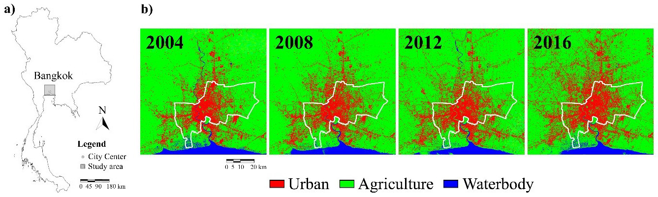
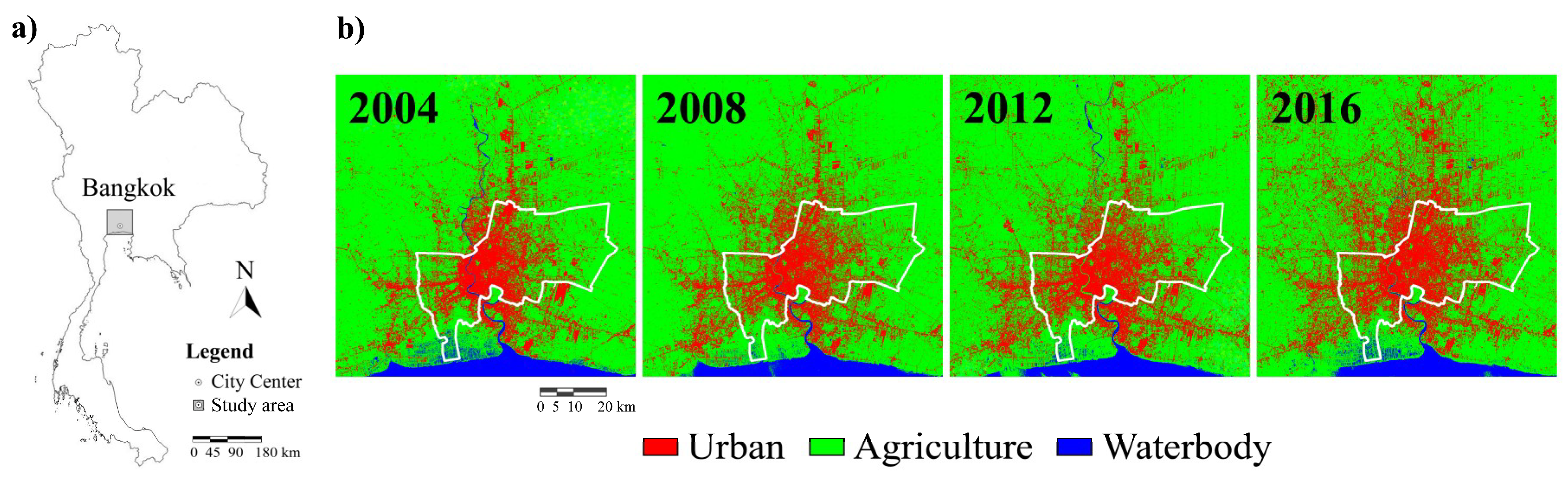
Land Use and Land Cover (LULC) maps of the Bangkok area (90 km × 90 km) for years 2004, 2008, 2012, and 2016, see Figure 1b, were retrieved by processing eight cloud-free images of reflective data measured by a Landsat-7 Enhanced Thematic Mapper Plus (ETM+) and Landsat-8 Operational Land Imager (OLI) and are reported in Table 1. Each Landsat platform covers the same area every 16 days.
These images, with reflective bands in the visible, near-infrared, and short-wavelength infrared and a spatial resolution of 30 m, were downloaded from the US Geological Survey (USGS) archive [26]. The Fast Line-of-sight Atmospheric Analysis of Hypercubes (FLAASH) atmospheric correction model embedded in the ENVI 4.5 software was applied.
The LULC maps provide three types of land cover, namely built-up (or urban), agricultural, and water body classes, derived by a supervised maximum likelihood classification approach using ENVI 4.5 [27,28]. The LULC map accuracy was evaluated by selected sites in Google Earth Pro high-resolution images, providing a Kappa coefficient of 0.81, 0.91, 0.87, and 0.83 for the land cover maps of 2004, 2008, 2012, and 2016, respectively, and an overall accuracy of 89% as a mean value for the four maps.
3.2. MODIS Data
Products from a MODIS sensor onboard Terra and Aqua satellites were employed to map the land surface temperature over the area of interest, downloaded from the Oak Ridge National Laboratory Distributed Active Archive Center (ORNL DAAC) website [29]. Both Landsat and MODIS products are projected into the Universal Transverse Mercator (UTM)-WGS 84 coordinate system. MOD11A2 (Terra) and MYD11A2 (Aqua) eight-day LST products, having 1-km spatial resolution, were used. These LST images consist of daily 1-km LST values averaged over an eight-day period. For the LST retrieval from MODIS observations, a split-window algorithm in clear-sky conditions is adopted, producing an accuracy better than 1 K [30]. Cloudy pixels in each image are masked out.
In this study we excluded the LST products during the rainy/monsoon season (May–October), having very few cloud-free images. Therefore, within each year LST maps during the winter season (November–January) and the summer season (February–April) were considered.
Terra satellite passes over Thailand at approximately 10:00 a.m. and 22:00 local time; Aqua satellite at around 14:00 and 2:00 a.m. (local time is +7:00 from UTC time).
Overall, we considered all the winter and summer MODIS LST images for the four years selected, i.e., 2004, 2008, 2012, 2016: A total of 237 clear-sky images (81, 37, 50, and 69 for 2004, 2008, 2012, and 2016, respectively) were processed. Specifically, for each year, all the images were divided into daytime (10:00 and 14:00) and night-time (22:00 and 02:00). Then, they were averaged producing two mean LST images over Bangkok. In this way, a mean LST pattern for each specific year is available, with night-time and daytime considered separately, at a 1-km spatial resolution. As an example, Figure 2 reports the two average maps for 2004 and 2016.
4. Methods
4.1. Urban Land Density Computation
An urban area is constituted by impervious surfaces and urban vegetation zones, the former represented by a built-up environment dominating the urban texture. The main urban area for a city includes the urban center or urban core, the inner suburban zones, and the outskirts.
In this study, a standardized approach for defining the spatial extent of a city and the urban land density was applied: It is based on a concentric ring partitioning, as described in [31,32], a method with a limited bias [23].
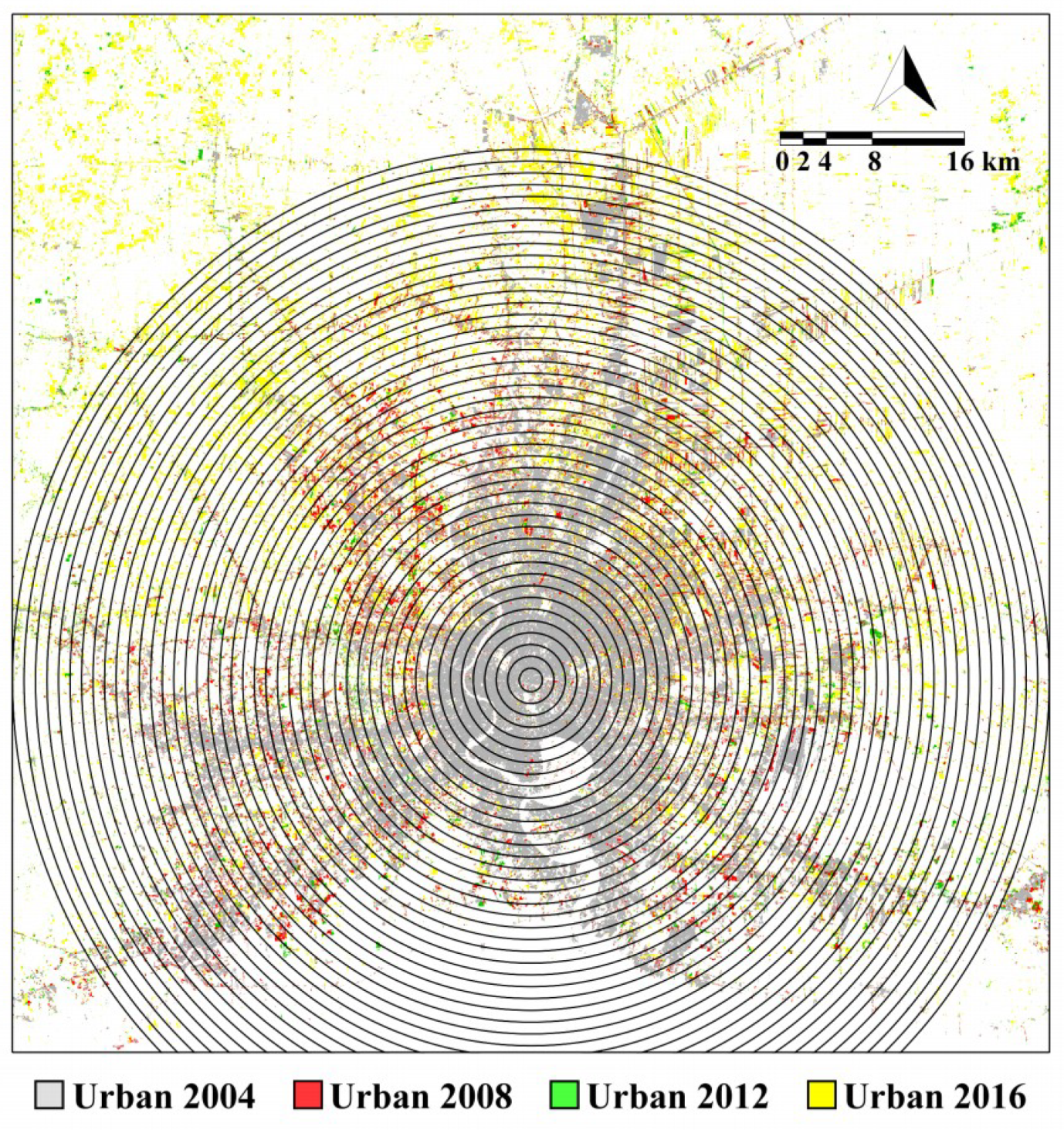
Therefore, once the study area center has been identified, Bangkok city was partitioned into a series of concentric rings 1-km wide, expanding outward starting from the center. The outer ring, representing the urban fringes (outside border), was selected to comprise metropolitan area outskirts that show a certain continuity of built-up surface presence.
The concentric partition of Bangkok is shown in Figure 3. The city center (latitude 13°45′7″N, longitude 100°31′48″E) is positioned in the commercial core zone; overall, Bangkok exhibits a monocentric urban expansion. For the four years 2004-2008-2012-2016, the urban land density in each ring was computed considering the pixels classified as “urban” in the LULC Landsat maps, i.e., dividing the area of the urban land by the total land area of the ring. Water pixels were discarded in the density computation [23].
From Figure 3, we can see that the missing part of the rings in the bottom is located over the sea, and therefore not considered in the density computation.
4.2. Inverse S-Shape Function
The spatial variation of urban land density as a function of the distance from the city center can be described by a modified sigmoid function exhibiting an inverse S-shape as reported in [23]
where: f is the urban density, r is the distance from the city center; c is a constant, asymptote of f, representing the background value of the urban built-up density in the outskirts (or hinterland) of the city. When c increases, it means that manmade surfaces in the hinterland grow due to the urban development of the study area; α is a constant controlling the slope of the density function; D is a constant estimating the radius of the main urban area. When D increases with time, it indicates the expansion of the urban area for a city.
The parameter interpretation is reliable when a monocentric urban expansion is assumed, as for Bangkok; for multinucleated cities such urban density fitting is not suitable.
As theoretically demonstrated in [23], significant parameters to evaluate the compactness of a city can be derived from Equation (1). The compactness refers to a high urban density in the city core and to a sharp reduction in the areas surrounding the core: Compact cities have f(r) with a steep slope, whilst for sprawling cities f(r) is clearly less steep. The f(r) slope, kS, computed in the intermediate urban zone between the city core and the urban fringes, is defined as [23]:
The kS (1/km) value is prone to decrease when the city exhibits an expansive urban growth.
4.3. Model Parameter Evaluation
In order to fit the function f(r) to the selected data, a nonlinear least-squares fitting method was applied. This approach fits the nonlinear model in Equation (1) to the data by estimating and refining the coefficients c, α, and D using an iterative process. The nlinfit function of the Statistic Toolbox of MATALAB R2015a, based on an iterative least-squares estimation, was employed to compute the f(r) parameters shaping the urban density curve for each year.
The same nlinfit function is also used for the parameterization of different nonlinear fitting models, as reported in Section 5.
4.4. Normalized LST
The application of the ring analysis to the temperature maps provides a mean LST trend versus distance as well as urban land density. To compare data from images of different years and seasons, considering the inter-annual variability of the atmospheric conditions, the LST for each pixel is scaled between the maximum and minimum values obtaining the normalized LSTn by the relation [33]:
where LST is the land surface temperature of a pixel, LSTmax and LSTmin are the maximum and minimum values of the study area for a specific scene. LSTn, computed to reduce the atmospheric condition effects for multi-year maps, is not an absolute surface temperature, but a generalized measure represented by an index between 0 and 1 (as the urban density) describing the variation pattern of the surface heating.
In this work, first the LSTn pattern from the eight mean LST maps of 2004, 2008, 2012, and 2016 is computed. Then, the mean daytime and night-time LSTn in each 1-km wide ring of Figure 3, discarding the water pixels, is produced. In the next section, we will show the results of this approach, the modeling and the comparison with the urban land density variation.
5. Results
5.1. Urban Land Density Modeling
By using the approach shown in Figure 3, the urban land density variation with the distance from the city center is reported in in Figure 4 for the four years.
As expected, the urban density reduces away from the city center. Also, it grows with years especially in the intermediate urban areas and outskirts, with a more intense hinterland sprawl in 2016. The urban density has the maximum values in the first 8 km from the center where it does not change significantly during the years studied. The little dip at 3 km is ascribed to the presence of parks in the city core [10]. The urban land density versus distance exhibits a trend following an inverse S-shape function. Therefore, Figure 5 shows the results of the function fitting (Equation (1)) on the urban density data reported in Figure 4. The corresponding fitting parameters c, α, and D are reported as well as the coefficient of determination r2. The very high r2 values confirm the reliability of the model function in following the urban density variability.
The parameter c slightly increases in the period 2004–2012, with an evident rise in 2016, highlighting the clear growth of built-up density in the outskirts in the last period. An increase of D with time is also found, indicating the expansion of the main urban area radius.
The kS parameter, see Table 2, decreases as the year increases, suggesting an expansive suburban growth trend: The 2016 density function of Figure 5 shows a less steep slope with respect to previous years and therefore the built-up density, from the city core towards the hinterland, has a more smoothed reduction.
5.2. Normalized LST Modeling
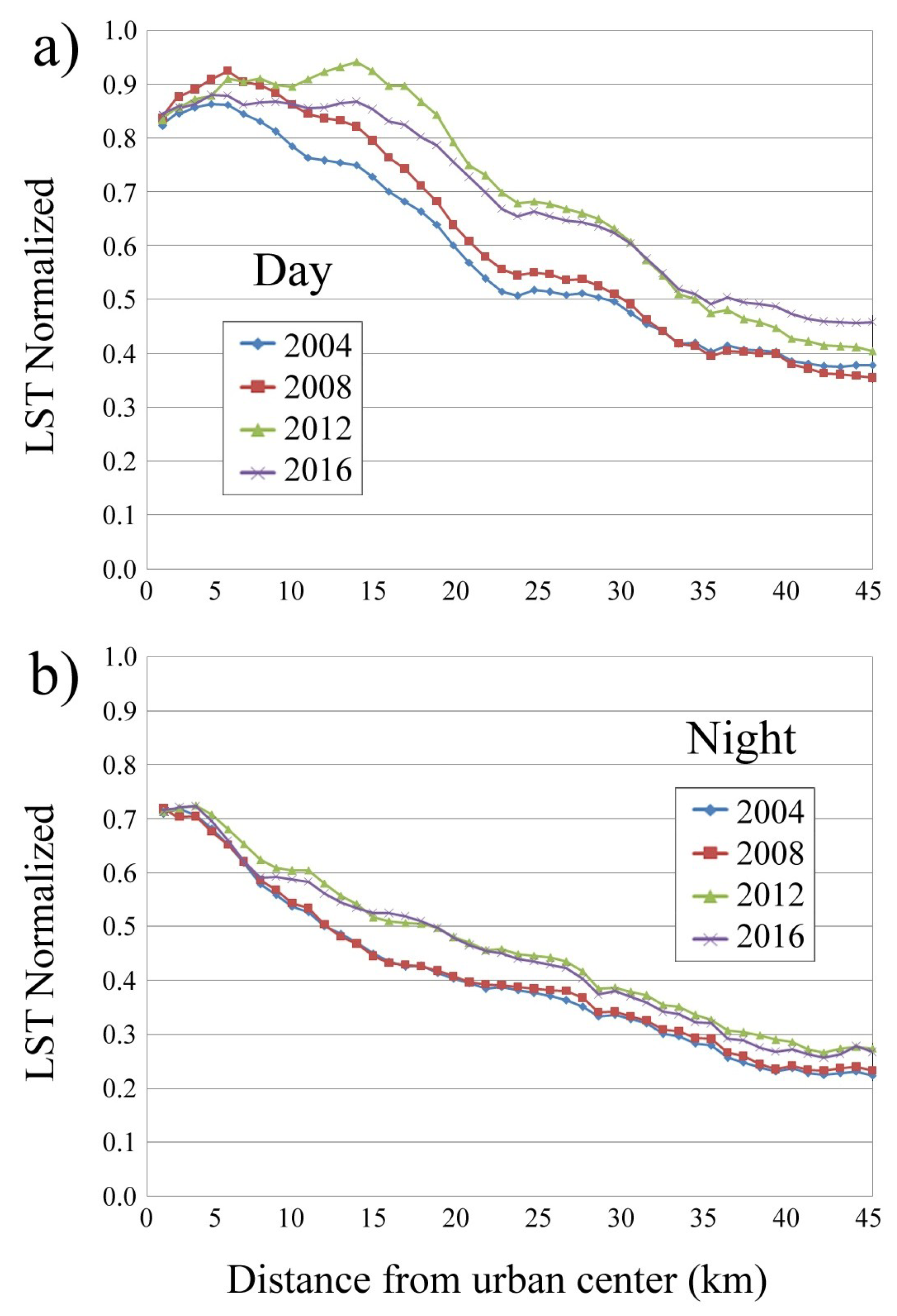
The mean LSTn as a function of the distance from the city center is computed for daytime and night-time, and is reported in Figure 6.
Even though the mean LSTn decreases away from the city center, daytime and night-time behavior is different in both values and shape. During the daytime, the LSTn values range from 0.4 to 0.9, whereas at night the range is between 0.2 and 0.7. The daytime LSTn for 2012 and 2016 keeps high values up to 18 km, whereas during the night high values are kept up to 4 km: This fact highlights a strong daytime urban heating expansion beyond the urban core in recent years, which is smoothed at night-time. Overall, the decreasing rate is more evident in the intermediate urban/suburban areas, whilst in the outskirts and urban fringes the diminishing trend is slighter.
In the first 8 km from the center, where the high urban land density has not exhibited significant changes during the years as shown in Figure 4, the daytime LSTn values are rather steady, whereas the night-time ones are stable in the first 4 km and decrease from 4 to 8 km, see Figure 6. This behavior suggests a perceptible night-time cooling effect in the outermost city core with respect to the first 4 km. The night-time LST growth with years arises from about 8 km from the city center up to the urban fringes, with similar values for the two pairs 2004–2008 and 2012–2016. Beyond 8 km, the daytime growth with years is more intense.
Concerning the fitting function for data of Figure 6, the daytime mean LSTn exhibits a trend that is again describable by an inverse S-shape function, whereas the night-time one follows a simpler quadratic function. Figure 7 shows the results of the function fitting, with the corresponding parameters and r2. The high r2 values prove the fitting reliability in describing the LST density variability.
The daytime inverse S-shape function features a LST growth in the urban fringes as proved by the rise of c in the last period. The kS parameters, shown in Table 3, are quite similar over the first three years; the lower kS value of 2016 indicates a daytime thermal expansion, also confirmed by the curve slope smoothing for 2016 in Figure 7a, showing a heating growth in the suburban areas and outskirts. This sprawling heating trend reflects the expansive suburban growth trend of Table 2. The outermost areas, if not densely urbanized, contain large rural zones which help reduce the warming rate of the outskirts and suburban zones, especially at night [34], as shown in Figure 7b.
5.3. Urban Density-LST Relationship
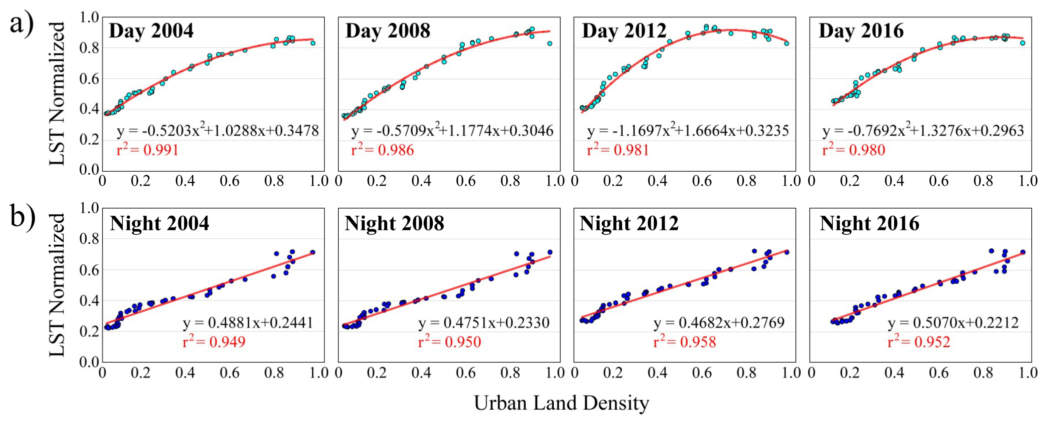
It is interesting to evaluate if the urban density data and the mean LSTn computed in each concentric ring show a distinct and accurate relationship. Figure 8 reports the yearly scatterplots for day and night, with the correspondent regression equations and r2.
For night-time, the fitting with the highest coefficient of determination is linear, with an r2 value of approximately 0.95–0.96, whereas for daytime it is quadratic, with an r2 value of approximately 0.98–0.99. The r2 values prove the efficiency of the relationship determined for urban density-LSTn, with the daytime one exhibiting a very high accuracy. It is important to notice that the LST normalization does not alter the curve behavior with respect to the ones not normalized, the latter providing the same coefficients of determination.
6. Discussion
The proposed research focuses on urban areas and surface heating patterns: the topic choice originates from the increasing interest in monitoring and prediction of the impact of heat events in worldwide cities, exposed to climate changes by global warming and localized urbanization effects such as the UHI [35].
Specifically, the first aim of this work is to compute the urban density and the mean LST curves as a function of the distance from the city center, and to model and parameterize them with fitting functions. In this way, clear and quantitative information regarding the urban density and LST behavior moving away from the city center is provided: the study can be easily replicated for other megacities exhibiting an urban growth across the years.
The results show that the Bangkok urban density curves are fitted by inverse S-shape functions with r2 equal to 0.99, reflecting the slight density decrease in the main city core and outskirts and the steeper slope in the intermediate urban areas; in Jiao [23], using the same ring approach and fitting function across 28 Chinese cities, the r2 values range between 0.88 and 0.99.
Concerning the surface temperature curve modelling, inverse S-shape and quadratic functions fitted the daytime and nighttime mean LSTn, respectively, highlighting the different heating mechanisms between day and night. The nighttime cooling effect just outside the 4-km ring, as detailed in Section 5.2, is not observed during daytime. Also, the daytime LST growth in the intermediate urban area is more intense. The day–night different shape may be ascribed to different factors. As reported in [10], the area surrounding the city core is constituted by residential, commercial and public zones: during the daytime, the intense human activities and the combined traffic congestion increase the surface warming, enlarging the heat island footprint [25]; during nighttime, due to the reduced working activities, a mitigation of the heating intensity and its footprint in such Bangkok zones is evident, as shown in [25]. The role of the anthropogenic heat release (e.g., air conditioning systems, energy use in transportation) as essential contributor to daytime urban warming due to intense human and economic activities is also confirmed in [6,36,37].
In this intermediate urban area, further investigations are needed to explain the highest surface temperature values for 2012 with respect to 2016. This behavior could be ascribed to changes over the years of the intrinsic factors underlying the urban heating dynamics (anthropogenic heat release, surface albedo and agricultural/rural classes), which affect the mean LST and may potentially explain the occasional crossings of the daytime yearly LSTn curves, unlike the urban density curves. In fact, the heat released from energy consumption can modify its intensity during the years, as well as changes in materials and albedo of pavement surfaces and building rooftops affect the thermal patterns [8,14]. Also, in the suburban areas and outskirts, the mean surface temperature is not only driven by the built-up area, but also by the agricultural classes that can experience changes during the years due to different crop practices. The surface transformations of agricultural classes implicate thermal condition variations (the more evident is for the bare soil-vegetation change). A more complete understanding of such LST variations needs an in-depth temporal and spatial investigation of these factors not analyzed here.
Anyway the study, carried out across the years both daytime and nighttime processing a great amount of MODIS images to encompass a multiplicity of surface thermal conditions, makes the research reliable and meaningful. In addition, the proposed model parameterization allows to identify how the suburban sprawl trend is reflected in a heating sprawl in the suburban areas. The analysis of the city compactness or dispersion, evaluated by the fitting function slope parameter, can be an index of the current and future thermal environment [38], providing a further indication for perspective urban developments. In fact, as reported in [38] for Beijing (China), numerical model experiments show that a dispersed city is efficient in mitigating the mean UHI intensity, but produces a larger regional warming effect spread out over the entire urban area compared to a compact city.
The second aim of the work is to infer the urban density-LST relationship. The accurate fitting results, confirmed by r2 ranging from 0.95 to 0.99, is obtained by a straightforward approach, providing an additional understanding of the relation between urban land density and heating effects, useful as a scientific support to a sustainable urban planning policy. An interesting comparison can be performed with the results reported in [39], where the relationship LST-impervious surface density was inferred by a ring-based approach in Bangkok, Jakarta (Indonesia), and Manila (Philippines), using data from a single Landsat-8 passage. A linear relationship was found, with r2 equal to 0.62, 0.92, and 0.82 for Bangkok, Jakarta and Manila, respectively, with greater dispersion in correspondence of the highest values of urban density. In our work such dispersion is less evident, since the annual mean mitigates the surface thermal variabilities. Morabito et al. [22], using mean LST from MODIS over a 13-year, observed linear relationships between built-up surface per km2 and LST for 4 Italian cities, with r2 in the range 0.57–0.77.
On the other hand, uncertainties and limitations remain in this research: first, the urban density and the mean LST are functions of the city center distance, but the ring-based analysis does not allow to identify if an evident directional anisotropy occurs. Second, the study examined the mean LST for clear days, whose values might be significantly larger than those in cloudy conditions, especially for surfaces with high solar radiation absorption. Although the applied LST normalization reduces the thermal variabilities, some effects could persist. Third, as previously pointed out, a more complete understanding of the LST anomalies in the yearly growth needs a detailed analysis and complementary data, both in time and space, of surface material changes, rural class modifications and human activity intensity. Finally, an investigation on the relationship between the mean LST trend and the city topography, e.g., the horizontal and vertical building distribution, is a further analysis that can improve the understanding of this topic.
7. Conclusions
Although the analysis of the impact of the urban land covers on the surface thermal pattern is widely addressed in literature, the application of the ring-based method to the two investigated dataset (built-up density and LST) allows to model and characterize them across the years as a function of the distance from the city center. Such standpoint provides a reliable fitting model of the two parameters and a straightforward and accurate relation between them.
The study is efficient and reliable for a city exhibiting a monocentric urban sprawl and, taking into account the daily/monthly variability of an urban LST pattern, it is important to process a great amount of satellite images if the study is aimed to provide a comparison across years (in this work 237 clear-sky MODIS scenes were processed). Moreover, this approach could be applied to other geophysical parameters retrievable from satellite images in order to evaluate their correlation with respect to the built-up density variability moving away from the city core. However, further investigations would improve this study: refinements in the ring-based approach for a potential anisotropy identification, comparison studies with other megacities in different parts of the world, analysis of the LST trend with the city topography.
Author Contributions
C.K. and S.B. conceived and designed the experiments; C.K. performed the experiments; C.K. and S.B. analyzed the data; S.B. wrote the paper.
Funding
This research was funded by the Department of Engineering of University of Perugia within the “Fondo di Ricerca di Base di Ateneo 2018”.
Conflicts of Interest
The authors declare no conflict of interest.
References
- Peng, S.; Piao, S.; Ciais, P.; Friedlingstein, P.; Ottle, C.; Bréon, F.M.; Nan, H.; Zhou, L.; Myneni, R.B. Surface urban heat island across 419 global big cities. Environ. Sci. Technol. 2011, 46, 696–703. [Google Scholar] [CrossRef] [PubMed]
- Anniballe, R.; Bonafoni, S.; Pichierri, M. Spatial and Temporal Trends of the Surface and Air Heat Island over Milan Using MODIS Data. Remote Sens. Environ. 2014, 150, 163–171. [Google Scholar] [CrossRef]
- Fallmann, J.; Forkel, R.; Emeis, S. Secondary Effects of Urban Heat Island Mitigation Measures on Air Quality. Atmos. Environ. 2016, 125, 199–211. [Google Scholar] [CrossRef]
- Chen, W.; Zhang, Y.; Pengwang, C.; Gao, W. Evaluation of Urbanization Dynamics and Its Impacts on Surface Heat Islands: A Case Study of Beijing, China. Remote Sens. 2017, 9, 453. [Google Scholar] [CrossRef]
- Bhargava, A.; Lakmini, S.; Bhargava, S. Urban Heat Island Effect: It’s Relevance in Urban Planning. J. Biodivers. Endanger. Species 2017. [Google Scholar] [CrossRef]
- Liao, W.; Liu, X.; Wang, D.; Sheng, Y. The Impact of Energy Consumption on the Surface Urban Heat Island in China’s 32 Major Cities. Remote Sens. 2017, 9, 250. [Google Scholar] [CrossRef]
- Wiesner, S.; Bechtel, B.; Fischereit, J.; Gruetzun, V.; Hoffmann, P.; Leitl, B.; Rechid, D.; Schlünzen, K.H.; Thomsen, S. Is It Possible to Distinguish Global and Regional Climate Change from Urban Land Cover Induced Signals? A Mid-Latitude City Example. Urban Sci. 2018, 2, 12. [Google Scholar] [CrossRef]
- Bonafoni, S.; Baldinelli, G.; Verducci, P. Sustainable strategies for smart cities: Analysis of the town development effect on surface urban heat island through remote sensing methodologies. Sustain. Cities Soc. 2017, 29, 211–218. [Google Scholar] [CrossRef]
- Bechtel, B. A New Global Climatology of Annual Land Surface Temperature. Remote Sens. 2015, 7, 2850–2870. [Google Scholar] [CrossRef] [Green Version]
- Keeratikasikorn, C.; Bonafoni, S. Urban Heat Island Analysis over the Land Use Zoning Plan of Bangkok by Means of Landsat 8 Imagery. Remote Sens. 2018, 10, 440. [Google Scholar] [CrossRef]
- Fan, C.; Myint, S.W.; Kaplan, S.; Middel, A.; Zheng, B.; Rahman, A.; Huang, H.P.; Brazel, A.; Blumberg, D.G. Understanding the Impact of Urbanization on Surface Urban Heat Islands—A Longitudinal Analysis of the Oasis Effect in Subtropical Desert Cities. Remote Sens. 2017, 9, 672. [Google Scholar] [CrossRef]
- Taha, H. Urban Climates and Heat Islands: Albedo, Evapotranspiration, and Anthropogenic Heat. Energy Build. 1997, 25, 99–103. [Google Scholar] [CrossRef]
- Baldinelli, G.; Bonafoni, S.; Rotili, A. Albedo Retrieval from Multispectral Landsat 8 Observation in Urban Environment: Algorithm Validation by in situ Measurements. IEEE J. Sel. Top. Appl. Earth Obs. Remote Sens. 2017, 10, 4504–4511. [Google Scholar] [CrossRef]
- Gago, E.J.; Roldan, J.; Pacheco-Torres, R.; Ordóñez, J. The City and Urban Heat Islands: A Review of Strategies to Mitigate Adverse Effects. Renew. Sustain. Energy Rev. 2013, 25, 749–758. [Google Scholar] [CrossRef]
- Xu, Y.; Ren, C.; Cai, M.; Edward, N.Y.Y.; Wu, T. Classification of Local Climate Zones Using ASTER and Landsat Data for High-Density Cities. IEEE J. Sel. Top. Appl. Earth Obs. Remote Sens. 2017, 10, 3397–3405. [Google Scholar]
- Weng, Q. Thermal infrared remote sensing for urban climate and environmental studies: Methods, applications, and trends. ISPRS J. Photogramm. Remote Sens. 2009, 64, 335–344. [Google Scholar] [CrossRef]
- Quattrochi, D.A.; Luvall, J.C. Thermal infrared remote sensing for analysis of landscape ecological processes: Methods and applications. Landsc. Ecol. 1999, 14, 577–598. [Google Scholar] [CrossRef]
- Zhao, G.; Dong, J.; Liu, J.; Zhai, J.; Cui, Y.; He, T.; Xiao, X. Different patterns in daytime and nighttime thermal effects of urbanization in Beijing-Tianjin-Hebei urban agglomeration. Remote Sens. 2017, 9, 121. [Google Scholar] [CrossRef]
- Ibrahim, F.G.R. Urban Land Use Land Cover Changes and Their Effect on Land Surface Temperature: Case Study Using Dohuk City in the Kurdistan Region of Iraq. Climate 2017, 5, 13. [Google Scholar] [CrossRef]
- Nurwanda, A.; Honjo, T. Analysis of Land Use Change and Expansion of Surface Urban Heat Island in Bogor City by Remote Sensing. ISPRS Int. J. Geo-Inf. 2018, 7, 165. [Google Scholar] [CrossRef]
- Ma, Q.; Wu, J.; He, C. A hierarchical analysis of the relationship between urban impervious surfaces and land surface temperatures: Spatial scale dependence, temporal variations, and bioclimatic modulation. Landsc. Ecol. 2016, 31, 1139–1153. [Google Scholar] [CrossRef]
- Morabito, M.; Crisci, A.; Messeri, A.; Orlandini, S.; Raschi, A.; Maracchi, G.; Munafò, M. The impact of built-up surfaces on land surface temperatures in Italian urban areas. Sci. Total Environ. 2016, 551–552. [Google Scholar] [CrossRef] [PubMed]
- Jiao, L. Urban land density function: A new method to characterize urban expansion. Landsc. Urban Plan. 2015, 139, 26–39. [Google Scholar] [CrossRef]
- Department of Public Works and Town & Country Planning. Available online: https://dpt.go.th/en/ (accessed on 12 September 2018).
- Keeratikasikorn, C.; Bonafoni, S. Satellite Images and Gaussian Parameterization for an Extensive Analysis of Urban Heat Islands in Thailand. Remote Sens. 2018, 10, 665. [Google Scholar] [CrossRef]
- US Geological Survey USGS. Available online: http://earthexplorer.usgs.gov (accessed on 11 September 2018).
- Bolstad, P.V.; Lillesand, T.M. Rapid Maximum Likelihood Classification. Photogramm. Eng. Remote Sens. 1991, 57, 67–74. [Google Scholar]
- Phiri, D.; Morgenroth, J. Developments in Landsat Land Cover Classification Methods: A Review. Remote Sens. 2017, 9, 967. [Google Scholar] [CrossRef]
- Distributed Active Archive Center DAAC ORNL. Available online: https://daac.ornl.gov/get_data/ (accessed on 12 September 2018).
- Wan, Z. New refinements and validation of the MODIS land-surface temperature/emissivity products. Remote Sens. Environ. 2008, 112, 59–74. [Google Scholar] [CrossRef]
- Wolman, H.; Galster, G.; Hanson, R. The fundamental challenge in measuring sprawl: Which land should be considered? Prof. Geogr. 2005, 57, 94–105. [Google Scholar]
- Schneider, A.; Woodcock, C.E. Compact, dispersed, fragmented, extensive? A comparison of urban growth in twenty-five global cities using remotely sensed data, pattern metrics and census information. Urban Stud. 2008, 45, 659–692. [Google Scholar] [CrossRef]
- Carlson, T.N.; Arthur, S.T. The impact of land use—Land cover changes due to urbanization on surface microclimate and hydrology: A satellite perspective. Glob. Planet. Chang. 2000, 25, 49–65. [Google Scholar] [CrossRef]
- Zhou, D.; Li, D.; Sun, G.; Zhang, L.; Liu, Y.; Hao, L. Contrasting effects of urbanization and agriculture on surface temperature in eastern China. J. Geophys. Res. Atmos. 2016, 121, 9597–9606. [Google Scholar] [CrossRef]
- McCarthy, M.P.; Best, M.J.; Betts, R.A. Climate change in cities due to global warming and urban effects. Geophys. Res. Lett. 2010, 37. [Google Scholar] [CrossRef] [Green Version]
- Du, H.; Wang, D.; Wang, Y.; Zhao, X.; Qin, F.; Jiang, H.; Cai, Y. Influences of land cover types, meteorological conditions, anthropogenic heat and urban area on surface urban heat island in the Yangtze River Delta Urban Agglomeration. Sci. Total Environ. 2016, 571. [Google Scholar] [CrossRef] [PubMed]
- Shahmohamadi, P.; Che-Ani, A.I.; Etessam, I.; Maulud, K.N.A.; Tawil, N.M. Healthy Environment: The Need to Mitigate Urban Heat Island Effects on Human Health. Procedia Eng. 2011, 20, 61–70. [Google Scholar] [CrossRef]
- Yang, L.; Niyogi, D.; Tewari, M.; Aliaga, D.; Chen, F.; Tian, F.; Ni, G. Contrasting impacts of urban forms on the future thermal environment: Example of Beijing metropolitan area. Environ. Res. Lett. 2016, 11. [Google Scholar] [CrossRef]
- Estoque, R.C.; Murayama, Y.; Myint, S.W. Effects of landscape composition and pattern on land surface temperature: An urban heat island study in the megacities of Southeast Asia. Sci. Total Environ. 2017, 577, 349–359. [Google Scholar] [CrossRef] [PubMed]
Figure 1.
(a) Bangkok position in Thailand (city center coordinates: latitude 13°45′7″N, longitude 100°31′48″E). (b) Land Use and Land Cover (LULC) map of Bangkok (90 km × 90 km) obtained from Landsat data for 2004, 2008, 2012, and 2016 (see Section 3.1). The white line is the Bangkok administrative boundary.

Figure 2.
Daytime and night-time average land surface temperature (LST) (°C) in 2004 and 2016 from MODIS.
Figure 2.
Daytime and night-time average land surface temperature (LST) (°C) in 2004 and 2016 from MODIS.
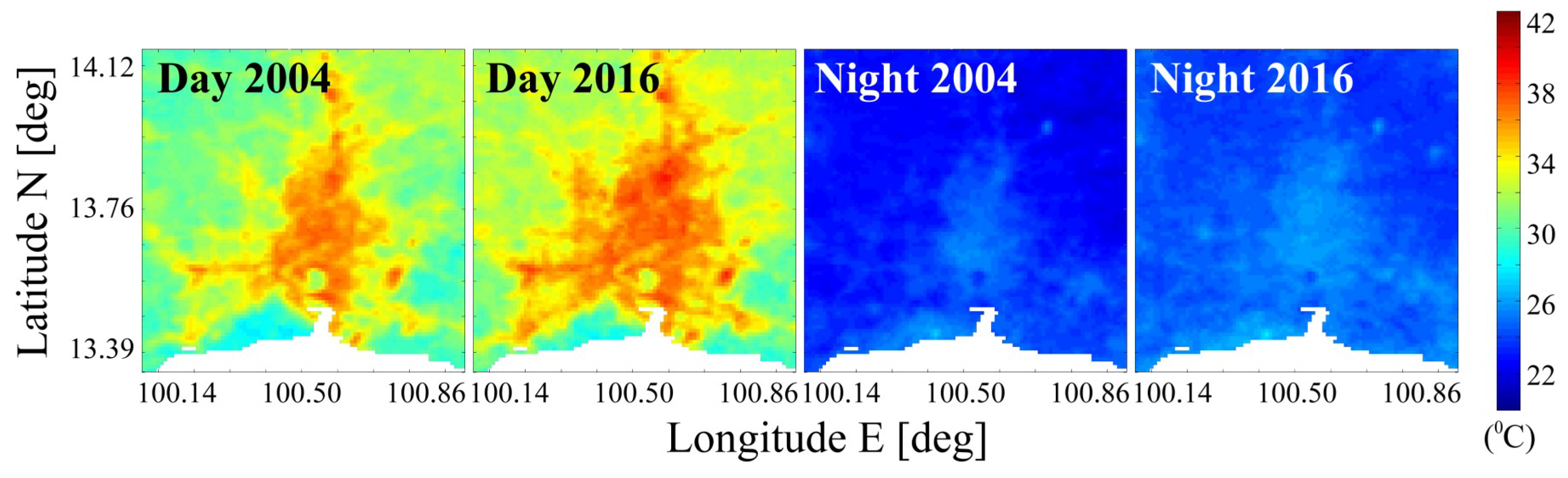
Figure 3.
The concentric ring-based partitioning of Bangkok for the four years. Ring distance is 1 km.
Figure 3.
The concentric ring-based partitioning of Bangkok for the four years. Ring distance is 1 km.

Figure 4.
Urban land density of Bangkok versus distance from the city center, for the years 2004, 2008, 2012, and 2016. LULC Landsat maps were used to select the “urban” category pixels.
Figure 4.
Urban land density of Bangkok versus distance from the city center, for the years 2004, 2008, 2012, and 2016. LULC Landsat maps were used to select the “urban” category pixels.
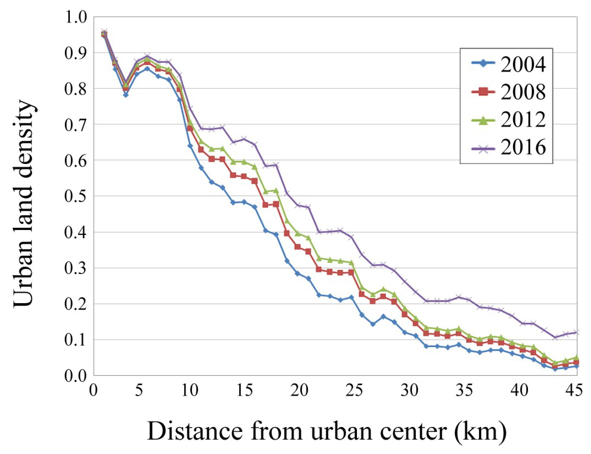
Figure 5.
Fitting of the land density data with the inverse S-shape function (Equation (1)) and corresponding parameters c, α, and D. The coefficient of determination r2 is reported.
Figure 5.
Fitting of the land density data with the inverse S-shape function (Equation (1)) and corresponding parameters c, α, and D. The coefficient of determination r2 is reported.
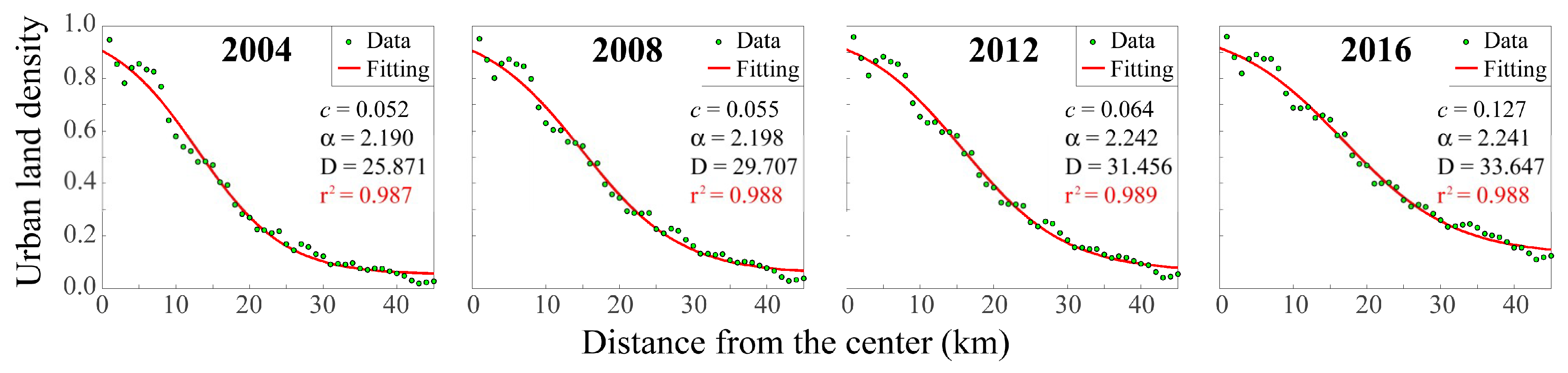
Figure 6.
Mean LSTn versus distance from the city center, for the years 2004, 2008, 2012, and 2016: (a) daytime; (b) night-time.
Figure 6.
Mean LSTn versus distance from the city center, for the years 2004, 2008, 2012, and 2016: (a) daytime; (b) night-time.

Figure 7.
Fitting of the mean LSTn data as a function of the city center distance. The r2 is also reported. (a) daytime: Inverse S-shape function and correspondent parameters c, α, and D.; (b) night-time: Quadratic function.
Figure 7.
Fitting of the mean LSTn data as a function of the city center distance. The r2 is also reported. (a) daytime: Inverse S-shape function and correspondent parameters c, α, and D.; (b) night-time: Quadratic function.
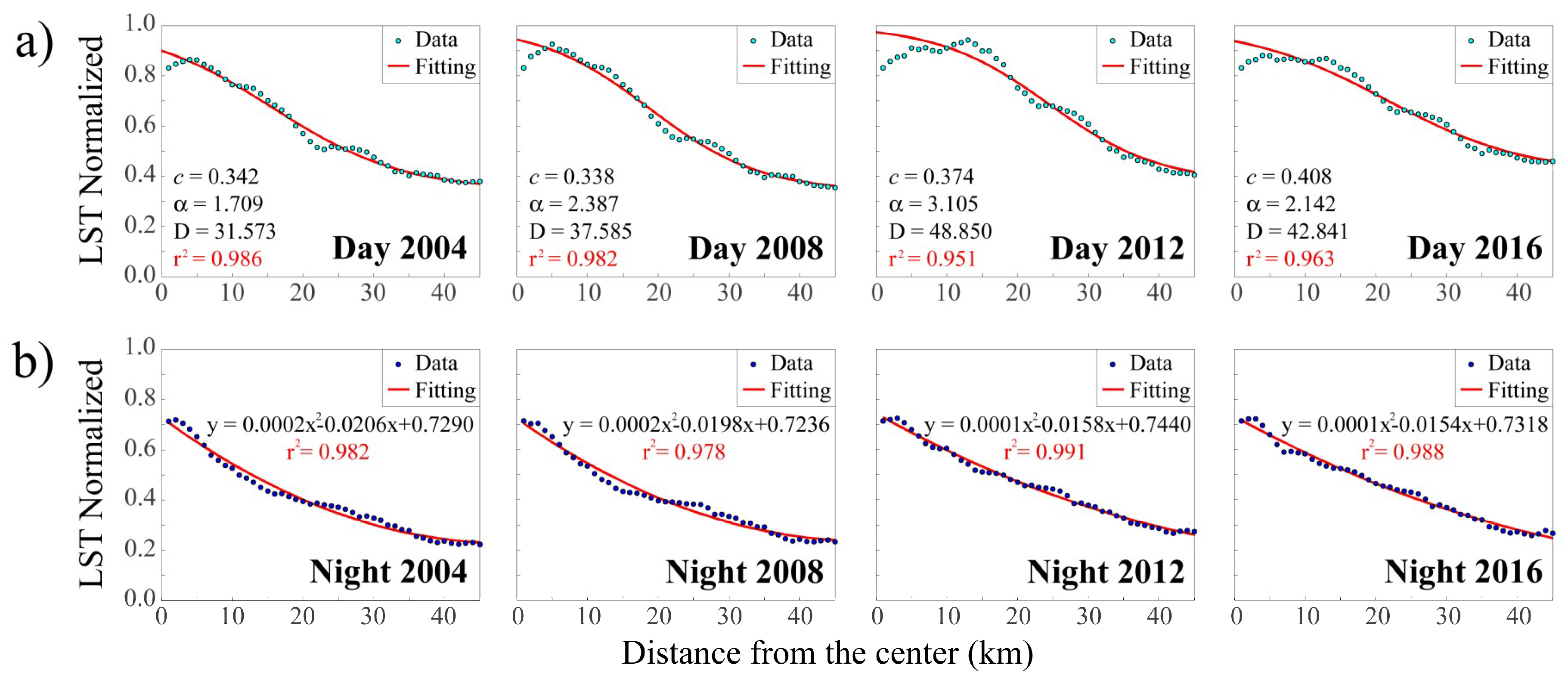
Figure 8.
Urban land density data versus LSTn computed in each concentric ring. Regression function and r2 are reported for each year. (a) daytime; (b) night-time.
Figure 8.
Urban land density data versus LSTn computed in each concentric ring. Regression function and r2 are reported for each year. (a) daytime; (b) night-time.

Table 1.
Landsat scenes used for Land Use and Land Cover (LULC) maps. WRS = Worldwide Reference System.
Table 1.
Landsat scenes used for Land Use and Land Cover (LULC) maps. WRS = Worldwide Reference System.
| No. | Date | WRS-2 Path/Row | Sensor |
|---|---|---|---|
| 1–2 | 31/12/2004 | WRS-2 129/50-51 | Landsat-7 ETM+ |
| 3–4 | 09/01/2008 | WRS-2 129/50-51 | Landsat-7 ETM+ |
| 5–6 | 11/05/2012 | WRS-2 129/50-51 | Landsat-7 ETM+ |
| 7–8 | 12/04/2016 | WRS-2 129/50-51 | Landsat-8 OLI/TIRS |
Table 2.
Slope parameter kS (1/km) for urban land density.
| 2004 | 2008 | 2012 | 2016 | |
|---|---|---|---|---|
| kS | 0.035 | 0.031 | 0.029 | 0.025 |
Table 3.
Parameter kS (1/km) for LSTn.
| 2004 | 2008 | 2012 | 2016 | |
|---|---|---|---|---|
| kS Day | 0.016 | 0.018 | 0.017 | 0.013 |
© 2018 by the authors. Licensee MDPI, Basel, Switzerland. This article is an open access article distributed under the terms and conditions of the Creative Commons Attribution (CC BY) license (http://creativecommons.org/licenses/by/4.0/).
Share and Cite
MDPI and ACS Style
Bonafoni, S.; Keeratikasikorn, C. Land Surface Temperature and Urban Density: Multiyear Modeling and Relationship Analysis Using MODIS and Landsat Data. Remote Sens. 2018, 10, 1471. https://doi.org/10.3390/rs10091471
AMA Style
Bonafoni S, Keeratikasikorn C. Land Surface Temperature and Urban Density: Multiyear Modeling and Relationship Analysis Using MODIS and Landsat Data. Remote Sensing. 2018; 10(9):1471. https://doi.org/10.3390/rs10091471
Chicago/Turabian StyleBonafoni, Stefania, and Chaiyapon Keeratikasikorn. 2018. "Land Surface Temperature and Urban Density: Multiyear Modeling and Relationship Analysis Using MODIS and Landsat Data" Remote Sensing 10, no. 9: 1471. https://doi.org/10.3390/rs10091471
Note that from the first issue of 2016, this journal uses article numbers instead of page numbers. See further details here.