SMOS Neural Network Soil Moisture Data Assimilation in a Land Surface Model and Atmospheric Impact

Abstract

The assimilation of Soil Moisture and Ocean Salinity (SMOS) data into the ECMWF (European Centre for Medium Range Weather Forecasts) H-TESSEL (Hydrology revised-Tiled ECMWF Scheme for Surface Exchanges over Land) model is presented. SMOS soil moisture (SM) estimates have been produced specifically by training a neural network with SMOS brightness temperatures as input and H-TESSEL model SM simulations as reference. This can help the assimilation of SMOS information in several ways: (1) the neural network soil moisture (NNSM) data have a similar climatology to the model, (2) no global bias is present with respect to the model even if local biases can remain. Experiments performing joint data assimilation (DA) of NNSM, 2 m air temperature and relative humidity or NNSM-only DA are discussed. The resulting SM was evaluated against a large number of in situ measurements of SM obtaining similar results to those of the model with no assimilation, even if significant differences were found from site to site. In addition, atmospheric forecasts initialized with H-TESSEL runs (without DA) or with the analysed SM were compared to measure of the impact of the satellite information. Although NNSM DA has an overall neutral impact in the forecast in the Tropics, a significant positive impact was found in other areas and periods, especially in regions with limited in situ information. The joint NNSM, T_2m and RH_2m DA improves the forecast for all the seasons in the Southern Hemisphere. The impact is mostly due to T_2m and RH_2m but SMOS NN DA alone also improves the forecast in July- September. In the Northern Hemisphere, the joint NNSM, T_2m and RH_2m DA improves the forecast in April–September, while NNSM alone has a significant positive effect in July–September. Furthermore, forecasting skill maps show that SMOS NNSM improves the forecast in North America and in Northern Asia for up to 72 h lead time.

1. Introduction

The amount of moisture in the soil is an important variable to understand the coupling of the continental surface and the atmosphere [1,2]. Soil moisture (SM) initialization is also crucial for seasonal forecasting studies since anomalies may persist at monthly to seasonal time-scales [3]. Local studies have shown the interest of assimilating in situ measurements of SM [4]. However, SM in situ measurements are too scarce at the global scale. Satellite remote sensing observations have their own limitations such as a limited accuracy and relatively long revisit times but they allow a global coverage.

The classical way to assimilate satellite observations is to use directly the satellite measurements [5,6,7]. Several experiments have been conducted to assimilate SM-related observations such as microwave brightness temperatures ($T_{\mathrm{b}}$s). For instance, the launch of the Soil Moisture and Ocean Salinity (SMOS) satellite [8] in November 2009 has offered global L-band (1.4 GHz) observations in polarimetry mode with multi-angular capabilities and a revisit time of three days or less. SMOS $T_{\mathrm{b}}$s are available in near-real-time (NRT) since the beginning of the mission. The assimilation of SMOS $T_{\mathrm{b}}$s has been used to constrain hydrological models [5,6]. The assimilation of SMOS $T_{\mathrm{b}}$s into a numerical weather prediction (NWP) forecasting system is however a complex task. The $T_{\mathrm{b}}$s assimilation requires the implementation of an observation operator going from SM to multi-angular and dual-polarization $T_{\mathrm{b}}$s in the top of the atmosphere using approximative radiative transfer computations [7,9,10]. In fact, one admitted advantage of assimilating $T_{\mathrm{b}}$s is that they have relatively well-defined associated instrument uncertainties. However, the assimilation of $T_{\mathrm{b}}$s requires not only the instrument noise, but also the radiative transfer uncertainties which can be very hard to specify [11]. Another advantage is that $T_{\mathrm{b}}$s can be easily available in NRT, which makes their use possible in an operational system. However, a neural network approach was implemented recently by the European Space Agency to develop the SMOS NRT SM product [12].

The assimilation of SM instead of the $T_{\mathrm{b}}$s has also been studied in different contexts. For instance SMOS SMs have been assimilated into land surface-hydrological models over the Great Lakes basin [13] and Ouémé catchment in Benin [14], into the Noah land surface model of the NASA land information system [15], into the SVAT (Soil Vegetation Atmosphere Transfer) models [16,17], and in carbon-cycle models [18]. The two approaches (i.e., the assimilation of $T_{\mathrm{b}}$s or retrieved SMs) were compared using the Variable Infiltration Capacity (VIC) hydrological model in [6]. The best results were achieved by assimilating the SM measurements. The authors interpreted this result as a consequence of the difficulty to model and to bias-correct the $T_{\mathrm{b}}$s obtained from radiative transfer estimations. Assimilating retrieved SM instead of $T_{\mathrm{b}}$s seems therefore an interesting approach.

In an assimilation framework, the SM retrievals need to be re-scaled to remove biases (model versus observations) and to be relatively consistent with the model. The goal is to avoid model/observations differences that could introduce divergences in the assimilation process. A common technique used to achieve this goal is to transform a posteriori the Cumulative Density Function (CDF) of the retrieved SM to match the modelled SM CDF [19,20]. However, when the two CDFs, computed at the pixel level, are matched (also at pixel level) the satellite spatial information can be distorted significantly towards the model patterns. Alternatively, it has been proposed to use a neural network (NN) to link observables such as microwave $T_{\mathrm{b}}$s or backscattering coefficients to model SM fields in particular from NWP models [21,22]. Such an approach has been developed to retrieve SM from SMOS observations [23]. An interesting property of the NN SM trained using modelled SM outputs is that, by construction, they share some statistical properties with the modelled SMs. For instance, they have no global bias with the reference SM. Both SMs (model and retrieved ones) show a similar climatology, even if they can have significant regional differences [24]. This is due to the fact that the “NN calibration” is performed globally. In fact, once trained, the NN output SM is driven only by the satellite observations and can be different to the SM predicted by the model. The overall NN methodology has been proposed to compute SM fields for an efficient data assimilation in [21,22].

The analysis of the SM has been conducted in the past jointly with near surface variables such as T_2m and RH_2m (hereafter called the “Screen Level Variables” or SLV). For instance, it has been shown that it is possible to jointly assimilate aircraft $T_{\mathrm{b}}$s and SLVs (T_2m and RH_2m), and that this approach gives more consistent results than assimilating $T_{\mathrm{b}}$s and SLVs separately [25]. Several data assimilation (DA) techniques (see [26] for a general description of DA techniques) have been compared: the optimal interpolation (OI), the two-dimensional variational assimilation (2D-VAR), or a Simplified Extended Kalman Filter (SEKF, with constant error covariance matrix). The SEKF technique improves the boundary layer forecasting skill [27,28,29,30,31] and it gives SM increments as a function of soil depth that are more realistic than those obtained using OI. This SEKF approach also brings a consistent improvement on SLV and SM forecasts, while allowing for an easier assimilation of satellite observations [20,30,32]. Since T_2m and RH_2m are not always representative of the SM content, it is also interesting to assimilate directly SM information to assess its individual information content. The assimilation of TMI (TRMM Microwave Imager) SM gave accurate estimates when compared to in situ observations and it influenced local weather parameters including the planetary boundary layer height and cloud coverage [33]. The assimilation of ERS SM index increased the correlation (and decreased the root mean square error) with respect to the Oklahoma Mesonet in situ measurements [34]. The corresponding forecasts for T_2m and RH_2m improved only marginally compared to the control experiment. The current operational system at ECMWF uses a SEKF joint analysis of T_2m, RH_2m and SM index from the Advanced Scatterometer (ASCAT) and show a neutral impact on both SM and SLVs [20].

The goal of this study is to perform DA experiments to analyse SM using a SMOS SM dataset obtained with a NN trained on the ECMWF land surface model and to evaluate its impact in NWP. Three configurations were tested: (1) a control experiment with no DA (hereafter “open loop”), (2) a configuration with NNSM-only (SMOS neural network soil moisture) data assimilation, and (3) a joint NNSM plus SLVs data assimilation. Experiments were conducted at the global scale and over a full year to determine where and when SMOS SM information improves the forecast.

This paper is organized as follows. Section 2 describes the remote sensing, in situ, and model data considered in this paper. Section 3 discusses the NN approach used to obtain SM from SMOS $T_{\mathrm{b}}$s, the DA framework and the evaluation methodology. Section 4 presents the results of the SM analysis using SLVs and NNSM. It also discusses the impact on atmospheric forecasts. The results are discussed in the context of other published works in Section 5. Finally, Section 6 summarizes the results and the conclusions.

2. Data

2.1. SMOS Level 3 Brightness Temperatures

SMOS was launched by ESA in November 2009 to monitor key elements of the water cycle [8]. It has a Y-shaped radiometer with 69 antennas that are used in interferometric mode to synthesize an aperture of ∼7.7 m. The spatial resolution on the ground varies from ∼30 km to ∼60 km across the field of view and it is 43 km on average. SMOS measures the thermal emission from the Earth at 1.4 GHz in full polarization and for incidence angles from 0${}^{\circ }$ to 60${}^{\circ }$. The revisit period is three days at the equator and decreases with increasing latitude. Equator overpass time is 6:00 (solar local time) for ascending overpasses and 18:00 (solar local time) for descending overpasses.

This study made use of the L3TB brightness temperature product [35] by the French SMOS ground segment CATDS (Centre Aval de Traitement de Données SMOS) because L3TB brightness temperatures are provided averaged in incidence angle bins of $5^{\circ }$-width and with polarizations referred to the Earth reference system (horizontal and vertical, H and V). L3TB data are provided on a 25-km Equal Area Scalable-Earth Grid (EASE grid) version 2 [36] as two daily products for ascending and descending overpasses (MIR_CDF3TA and MIR_CDF3TD products, respectively). The version of the data used in this study is version 310.

2.2. HTESSEL Model Data

The land surface model used in this study is the “Tiled ECMWF Scheme for Surface Exchanges over Land” (TESSEL) with improved land surface hydrology (H-TESSEL) [37]. The improvements include a new soil hydrology with more realistic runoff, a revision of the snow parametrisation and the bare ground evaporation and a monthly varying climatology of leaf area index (LAI) based on MODIS data [38,39,40]. H-TESSEL uses four soil layers. The depths of the three top soil layers are 0–7 cm, 7–28 cm, and 28–100 cm. The ECMWF Integrated Forecast System (IFS) uses a spectral representation of meteorological fields where each field is expanded in series of spherical harmonics. The spatial resolution is determined by the truncation of the series at a given total wavenumber. In this study, the model was run with a spectral truncation T511, since the equivalent spatial resolution of approximately 39 km is similar to that of SMOS. Following the ERA-Interim/Land [41] approach, H-TESSEL was forced with the near surface atmospheric fields obtained from the ERA-Interim re-analysis [42].

2.3. ECMWF Data Interpolated to the Grid of the SMOS Level 3 Brightness Temperatures Data Set

This study used the CATDS AUX_CDFECA and AUX_CDFECD products, which contain ECMWF IFS data re-sampled from a Gaussian N400 grid to the EASE grid of the SMOS L3TB product using a bilinear spatial interpolation and interpolated linearly in time to match the time of SMOS overpasses in between two consecutive 3 h forecasts. Therefore, we used those products to extract the volumetric moisture content in the first soil layer (0–7-cm depth; hereafter ECMWF SM${}_1$) to train the NNs. In addition, the snow depth and the soil temperature in the first layer were used to filter out regions with snow or frozen soils (see Section 3).

2.4. In Situ Measurements

Surface synoptic observations (SYNOP) of T_2m and RH_2m are used by NWP centers to analyse SM. First, a screen level analysis is performed, which provides gridded fields of analysed T_2m and RH_2m. Subsequently, these fields are used as input of the SM analysis [30,43]. This is the approach used in this study to assimilate SLVs.

In addition to data for assimilation, in situ measurements were also used for evaluation. The analysed SM fields discussed in this study, along with the model open loop (i.e., no DA), were evaluated against in situ measurements of SM for a large number of sites (>800 sites,

Table 1. In situ networks used in this study. The depths are quoted as two numbers: the first one is the upper depth, and the second one is the lower depth of the sensor. Both numbers are equal when the sensor is placed horizontally. The third column gives the number of sensors remaining for each network after applying all of the criteria used for the evaluation that are discussed in Section 2.4. The fourth column gives the average number of points in the time series for each network that satisfies the evaluation criteria.

Network	Depth (m)	Sensors	N${}_{\mathit{points}}$	Location	Reference
DAHRA	0.05–0.05	1	1137	Senegal	[45]
REMEDHUS	0.00–0.05	23	1016	Spain	[46]
SMOSMANIA	0.05–0.05	19	1009	France	[47]
HOBE	0.00–0.05	46	687	Denmark	[48]
PERUGIA	0.05–0.05	2	719	Italy	[49]
FMI	0.05–0.05	8	245	Finland	...
SCAN	0.05–0.05	240	816	USA	[50]
SNOTEL	0.05–0.05	347	537	USA	[51]
USCRN	0.05–0.05	122	931	USA	[52]
ARM	0.05–0.05	31	717	USA	...
PBO-H2O	0.00–0.05	101	206	USA	[53]
CTP-SMTMN	0.00–0.05	33	365	China	[54]

). All of the in situ data were obtained from the International Soil Moisture Network [44]. Since the microwave radiation detected from space comes from the first few centimeters of the soil, only SM measurements at depth ranges from 0 to 5 cm (vertical sensors) and ∼$5\pm 1$ cm (horizontal sensors) were used. The sites are located in four continents and cover a large spectrum of climate conditions. Table 1 shows a summary of the networks used, including the depth of the measurement, the location and the number of sensors.

3. Methods

Figure 1 shows a flow chart of the SMOS NNSM data assimilation and the evaluation methodology, which can be divided in three main blocks. First, instead of implementing an observation operator computing the radiative transfer from SM to $T_{\mathrm{b}}$s, here, the NN is trained to find a non-linear mapping from $T_{\mathrm{b}}$s to SM. This is presented in detail in Section 3.1. Second, the NNSM data, with and without SLVs, are assimilated into H-TESSEL using the ECMWF surface-only Land Data Assimilation System (so-LDAS) as discussed in Section 3.2. Finally, the so-LDAS analysed SM fields were used to initialise atmospheric forecasts, allowing evaluation of the impact of SMOS NNSM DA on NWP as detailed in Section 3.4.

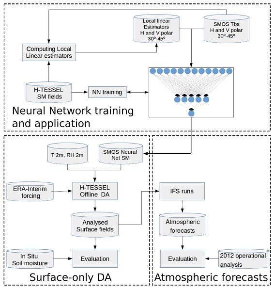
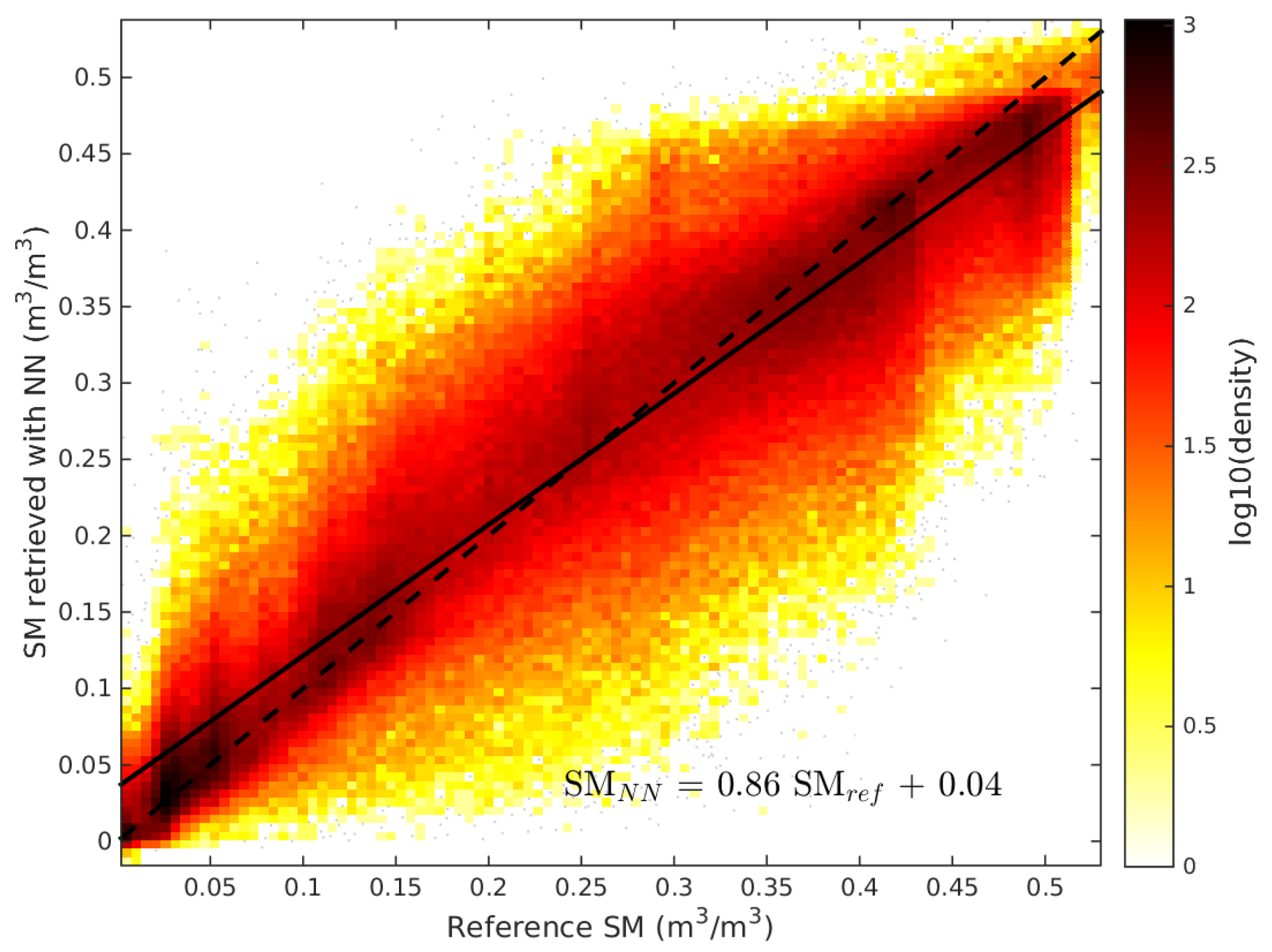
3.1. Using a Neural Network to Compute a New Soil Moisture Data Set

The reference data used to train the NN is ECMWF SM${}_1$ collocated in space and time with SMOS $T_{\mathrm{b}}$s (Section 2). In order to maximize the swath width of the SM retrieval and the quantity of data available for assimilation, only incidence angles from 30${}^{\circ }$ to 45${}^{\circ }$ were used, as for the ESA NRT SM product [12]. Twelve quantities were used as predictors to retrieve soil moisture: six $T_{\mathrm{b}}$s and six SM linear expectations (index $I_2$ in [12]) for two polarizations (H and V) and three angle bins (30–35${}^{\circ }$, 35–40${}^{\circ }$, 40–45${}^{\circ }$).

The training database was constructed using data from 10 November 2010 to 31 December 2013. The data were temporally sampled with a time step of 5 days. Finally, the data were also spatially sampled with a step of three grid points both in latitude and longitude. ECMWF H-TESSEL model estimations of snow depth and the temperature of the first soil layer were used to filter out regions with snow or frozen soils. In addition, SMOS data with a probability of being affected by artificial emission (radio frequency interferences) higher than 20% as given by the RFI_Prob parameter in SMOS Level 3 files were also filtered out.

From the filtered data subset, 60% of the samples were used for the actual NN training, 20% were used for evaluation of the training process and to avoid over-training, while the final 20% was used as a test set to evaluate the performance of the trained NN a posteriori. The training was done using gradient back-propagation and the Levenberg-Marquardt algorithm [55]. A two layer NN with one hidden layer with 5 non-linear neurons and a second layer with one linear neuron was used as this architecture manages to capture the relationship between the input data and the target SM dataset while keeping the NN as simple as possible [12,23]. The training was stopped after 50 iterations when the mean squared difference was asymptotically approaching to a minimum without significant signs of over-training in the evaluation subset. The NN output uncertainty was computed taking into account the radiometric noise of the $T_{\mathrm{b}}$s and a 1% error for the extreme ECMWF SM${}_1$ values used to compute the local SM linear expectations $I_2$ (which is a conservative upper limit to the model background error used for the DA, which is shown in Figure 2).

Figure 3 shows a scatter plot of the SM estimated from the NN for the test subset with respect to ECMWF SM${}_1$. The Pearson correlation R of both data sets was 0.94, which imply a good ability of the NN to capture the dynamics of the ECMWF SM${}_1$ dataset. The standard deviation of the difference (STDD) was 0.054 m${}^3$m${}^{-3}$ and the Root Mean Square Error or Difference (RMSE) was also 0.054 m${}^3$m${}^{-3}$, which implies that there is not a significant bias in between both SM datasets.

Taking into account that the model surface SM was used as reference data for the NN training, it is pertinent to discuss whether this approach can introduce cross-correlated errors between the observations and the model. This was actually considered since the methodology was proposed [21]. Systematic errors of the model such as a possible global SM bias with respect to ground truth will also be present in the NN output. Nevertheless, this is not a problem since satellite data needs to be calibrated towards the model in order to be assimilated. Another issue could be possible regional errors (both biases and errors in the dynamics/climatology). However, Jimenez et al. [24] have shown that these regional errors are not reproduced by the NN because they do not affect the training. In summary, after the training stage, the NN output is a function of the input variables (satellite observations). Therefore, regional model errors are not reproduced since they are not present in the satellite observations and correlations between NNSM and model SM errors are not expected.

3.2. Offline Surface-Only Land Data Assimilation System

The data assimilation framework used in this study is the ECMWF surface-only Land Data Assimilation System (so-LDAS).

Table 2. Comparison of the IFS Land Data Assimilation System (LDAS) and the surface-only LDAS.

	IFS-LDAS	so-LDAS
Assimilation technique	SEKF	SEKF
Assimilation window	12 h	24 h
Surface-atmosphere coupling	fully coupled	uncoupled, surface forced by ERA-Interim
Observation input grid	Independent of the model grid	Same grid as the model grid
Analysis	RH2m, T2m, SM, soil temperature, snow cover and snow temperature	SM
Observation input	RH2m, T2m, ASCAT SM, LST, snow cover and snow temperature, SMOS TBs (in development)	RH2m and T2m analysed with IFS-LDAS, ASCAT SM, SMOS SM
Increment applied	analysis time	Initial time step and additional trajectory
Background error	0.01 m${}^3$m${}^{-3}$	5% of water holding capacity

summarizes the main differences of the so-LDAS and the LDAS of the Integrated Forecast System (IFS-LDAS). The so-LDAS was used for this study because it uses a similar point-wise Simplified Extended Kalman filter scheme as the IFS-LDAS [20] to perform a joint assimilation of analysed SLVs provided by the IFS-LDAS and remote sensing SM but allow carrying out long surface-only DA experiments faster than the IFS-LDAS. It is worth noting that the methodology of using NNs to link the satellite observables to model variables is independent of the actual DA technique and therefore it could also have been used within other DA frameworks such as Ensemble Kalman Filters or Particle Filters.

The so-LDAS relies on an offline sequential data assimilation in a 24-h window, based on the H-TESSEL land surface model [37] with ERA-Interim atmospheric forcing [42]. The control vector x has three elements corresponding to the SM from the three first soil layers of the model. For each observation within the assimilation window, the observation vector $y_o$ has one element when only NNSM is assimilated or three elements if T_2m and RH_2m are also assimilated. The analysis increments, $\Delta x$, are computed as the product of the Kalman gain matrix K and the innovations or first guest departures vector (difference of the model at time t, $y_t$, and the observation operator h applied to the control vector at time 0).

$$\Delta x=K(y^t-h\left(x^0\right))$$

(1)

The Kalman gain is computed as:

$$K=B{H}^T{(HB{H}^T+R)}^{-1}$$

(2)

where B is the background error covariance matrix, R is the observation error covariance matrix and H is the Jacobian of the observation operator, which is estimated by perturbing each component of the control vector. The observations are assimilated over a 24 h window divided in 1-h bins. The increments are applied at the beginning of the 24-h data assimilation window, as in the simplified 2D-VAR proposed by [29]. Following the approach of [31], for every 24-h analysis cycle, five trajectories of H-TESSEL are produced. The first trajectory provides the model background. Three more trajectories are produced by perturbing the soil moisture initial condition of the first, second and third layer, respectively. In the last trajectory the analysis increments are applied at the beginning of the 24-h window. It provides the analysed trajectory.

The matrix B is time-independent (simplified EKF). For each grid point, B is a diagonal matrix whose non-zero elements are the errors ${\sigma }_b$ of the three upper model layers, which were fixed to 5% of the water holding capacity, which is the difference between the volumetric field capacity and the wilting point. It is calculated for each layer and grid point as a function of soil type [56]. The model and the DA framework use volumetric SM in m${}^3$/m${}^3$ units. Figure 2 shows a global map of the model background error ${\sigma }_b$.

For each grid point, the observation error covariance matrix R is a diagonal matrix with elements ${\sigma }_{T_{2m}}$ (set to 1 K) and ${\sigma }_{R{H}_{2m}}$ (set to 4%) and ${\sigma }_{SM}$. The uncertainty of the NN output (${\sigma }_{NN}$) is variable in space and time but it is a lower limit to the actual observation error [12]. Therefore, in the context of this DA study ${\sigma }_{SM}$, was taken as three times the NN output error. The multiplicative factor used to compute ${\sigma }_{SM}$ was determined to obtain an average close to 0.05 m${}^3$/m${}^3$, which is the error used for the operational assimilation of ASCAT in the ECMWF IFS.. Figure 2 shows an example of ${\sigma }_{SM}$.

Table 3. Experiments compared in this study. Experiment labels are shown in column 1. Column 2 shows if SM is assimilated or not. Column 3 shows the observation error assumed for the SM dataset (${\sigma }_{SM}$) as a function of ${\sigma }_{NN}$, which is provided by the retrieval algorithm. Figure 2 shows an example of ${\sigma }_{NN}$. Column 4 shows if T_2m and RH_2m are also assimilated for each experiment.

Label	SM	${\mathit{\sigma }}_{\mathit{SM}}$	SLV
OL	no	...	no
NNSM	yes	$3\times {\sigma }_{NN}$	no
NNSM-SLV	yes	$3\times {\sigma }_{NN}$	yes
NNSM${}_{LW}$	yes	$9\times {\sigma }_{NN}$	no
SLV*	yes	$9\times {\sigma }_{NN}$	yes

summarizes the assimilation experiments conducted for this study. The first three experiments are the Open-Loop (OL, H-TESSEL without assimilation), “NNSM” and “NNSM-SLV”. In addition, two other experiments were carried out to evaluate the sensitivity of the DA to the observation error ${\sigma }_{SM}$ and the relative importance of NNSM and the SLVs for the assimilation: A low weight NNSM experiment “NNSM${}_{LW}$” was carried out multiplying ${\sigma }_{NN}$ by an additional factor of 3 with respect to the “NNSM” experiment. A “NNSM${}_{LW}$-SLV” experiment was also carried out. As discussed in Section 4 and Section 5, this experiment is close to the SLV-alone case, because the relative weight of the SM data for the assimilation is very low. Therefore, for simplicity it will be referred to in the following as SLV*.

3.3. Soil Moisture Analysis Evaluation against In Situ Measurements

The analysed fields and the model open loop have been evaluated against in situ measurements using the following protocol. Sites and times covered by snow and with frozen soil (first layer temperature lower than 274 K) were filtered out. The in situ measurements were compared to the closest model grid point. To select a given in situ measurement, a time window of ±30 min around the model time was used. Data from a given time are used to compute statistical metrics only if a SM value is available for all of the datasets shown in Table 3, ensuring that all time series contain exactly the same number of points, and there are at least 200 common points. Table 1 shows the number of sensors that satisfied the previous criteria for each network and the mean number of points in the time series. The STD and RMS of the difference time series were computed. The bias was computed as the mean of the analysed (or OL) times series minus the mean of the in situ measurement times series. Those metrics, in addition to the Pearson correlation, were computed sensor by sensor with respect to the closest grid point. Afterwards, the metrics were analysed site per site and network per network. The results are presented in Section 4.3.

3.4. Impact of the Soil Moisture Analysis on the Forecast

The OL and the analysed surface fields were used to initialise atmospheric forecast experiments at a T511 resolution (39 km) for the whole 2012. To evaluate the different forecasts, the following method was used. The analysis of the IFS that was operational in 2012 was used as reference and the different forecasts were compared to this reference in periods of three months. In a second step, the scores obtained for the forecast using the surface model with no DA were subtracted from the scores obtained for the forecasts using analysed surface fields. Therefore, negative values imply that the forecast using analysed SM are closer to the reference than the forecast with no surface assimilation. The results are discussed in Section 4.4. It is worth noting that the evaluation statistics are very robust as the forecast period is long and allows a detailed analysis for the different seasons.

4. Results

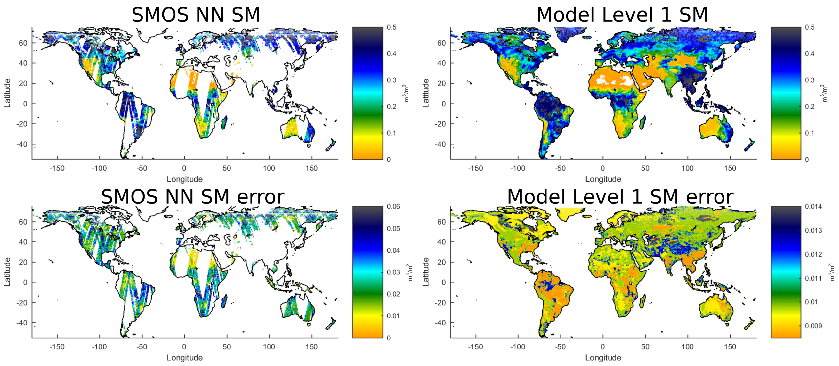
4.1. Observations and Model Comparison

Using the NN trained as explained in Section 3, a new SM dataset for the year 2012 was computed specifically for this DA experiment. Figure 2 shows an example of the NNSM data. By construction, the NNSM map is similar to the H-TESSEL map, but it shows small differences coming from the SMOS $T_{\mathrm{b}}$s and the trained NN. To get further insight into the data set to be assimilated, NNSM, RH_2m, and T_2m were compared systematically to the model simulations. Figure 4 shows the mean innovations (observations–model) for NNSM and RH_2m for January–March (JFM) and July–September (JAS). Figure 4 also shows the mean innovations for T_2m but computed as model–observations because the T_2m and SM relationship is, in principle, inverse (the more SM the lower T_2m, and conversely). In general, the innovations for the different observables are in good agreement. For instance, in North America, in all seasons, innovations show different signs on the west and east coasts with respect to the central region. All innovations are generally in good agreement in South America. However, some differences can also be seen for example in India and Australia in JFM, as they are in agreement for NNSM and RH_2m but not T_2m in India and they are in agreement for T_2m and RH_2m but not for NNSM in Australia. For a given observable, the sign of the innovations can change with time. For instance, innovations are negative for NNSM in Australia in JFM and positive in April-September (only JAS is shown in Figure 4). Innovations are also negative for NNSM and RH_2m in South America for most of the year except in JAS, when they are positive in large regions of this continent.

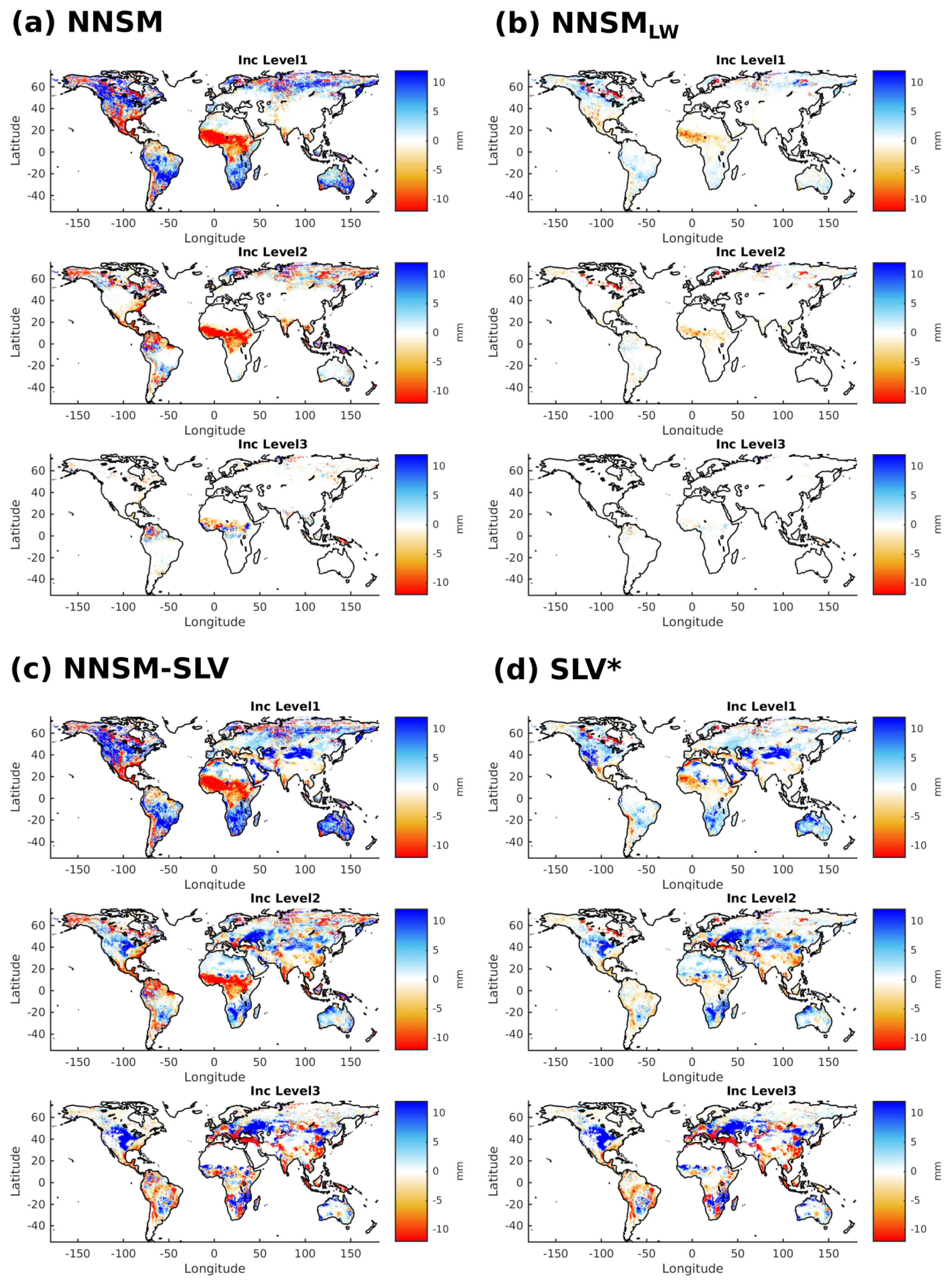
4.2. Data Assimilation

Figure 5a–d show the sum of the increments in the period from July to September for the four DA experiments. As expected, when the observation errors increase the increments decrease from ∼10 mm (NNSM) to values lower than ∼5 mm (NNSM${}_{LW}$) for the first model layer. For the first model layer, the increments show clear geographical patterns, being negative in the Sahel region and from the north of South America to the south of North America and positive elsewhere. The increments in the second model layer are smaller but still significant close to the Equator and at high northern latitudes. Finally, Figure 5b shows that when the observation error is high (NNSM${}_{LW}$), the low weight given to NNSM data during the assimilation makes that the impact is very low.

As expected, the third model soil layer increments are mainly due to SLV DA (see Figure 5a,c), while surface SM has more impact on the first layer (see Figure 5c,d). The effect of SLV DA is clear in comparing the results for NNSM${}_{LW}$ (Figure 5b) and SLV* (Figure 5d). As discussed above, in experiment NNSM${}_{LW}$ SM is almost not assimilated except in the Sahel and Northern Canada. Therefore, the most significant positive increments from SLV DA are present in central Asia and North America, while the DA removes moisture from the model third layer in parts of India, China, Europe and South America. It is noteworthy that the analysis of SLV gives positive increments in Asia in areas where SMOS data is not available due to contamination by artificial emission at 1.4 GHz (radio frequency interference, RFI).

The seasonal behaviour of the assimilation of NNSM is shown in Figure 6 for experiment NNSM. Cumulative increments in Australia, South Africa and parts of South America are negative in January-March and October-December and they are positive from April to September. This behavior is in agreement with NNSM innovations (Figure 4).

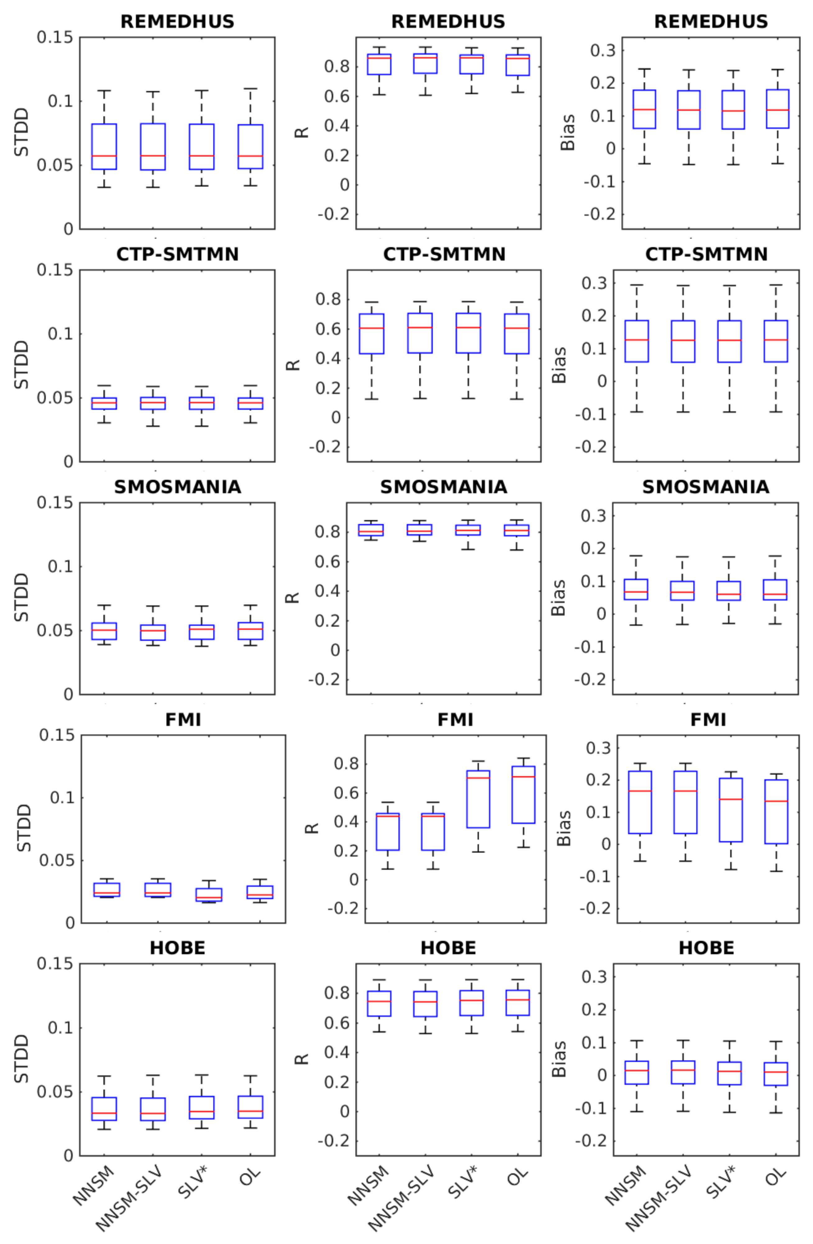
4.3. Evaluation of the Soil Moisture Analysis

The analysed soil moisture fields and the model open loop were compared to in situ measurements of SM in the surface layer (∼0–5 cm) for the sites discussed in Section 2 using the protocol presented in Section 3.3. Figure 7 and Figure 8 summarize the results as box plots computed network by network. On each box, the central mark indicates the median of the distribution and the bottom and top edges of the box indicate the 25th ($q_{25}$) and 75th ($q_{75}$) percentiles, respectively. The results for Dahra and Perugia are shown in

Table 4. Evaluation against in situ measurements. Mean standard deviation of the difference (STDD), Pearson correlation (R) and bias with respect to the in situ measurements for each network of in situ sensors.

	DAHRA			PERUGIA
	STDD	R	Bias	STDD	R	Bias
NNSM	0.048	0.71	0.112	0.057	0.79	0.079
NNSM-SLV	0.050	0.72	0.115	0.057	0.79	0.075
SLV*	0.054	0.72	0.118	0.057	0.79	0.075
OL	0.053	0.72	0.117	0.057	0.79	0.079

because they only have one and two sensors, respectively.

NNSM degrades the SM analysis at the Finish Meteorological Institute (FMI) site (Figure 7). The effect is seen consistently in R, which decreases, and $STDD$, which increases. In contrast, in the ARM network, NNSM and NNSM-SLV give better results than OL and SLV* in terms of $STDD$ (lower median, $q_{25}$ and q${}_{75}$) and R (higher median, $q_{25}$ and q${}_{75}$) with very similar bias. For all the other networks, including Dhara and Perugia, the distributions of $STDD$, R and bias for the NNSM, NNSM-SLV and SLV* experiments are similar to those of the OL run, except for SMOSMANIA, which shows a slightly lower median of R for NNSM and NNSM-SLV while showing also a slightly lower dispersion. Taking into account the low impact in the surface layer found at those locations and the low increments shown in the previous section for model layers 2 and 3 when assimilating only surface soil moisture, the comparison of model and in situ measurements for deeper layers was not studied further. The impact of SLV DA for lower layers is larger but this paper is mainly devoted to the NN approach to assimilate SMOS SM instead of SMOS Tbs. The impact of SLVs on deeper layers has been discussed in other studies [7,20,57].

Even if the distribution of the statistical metrics network by network is very similar for the analyzed fields with respect to the OL run, there are significant differences for some sites. Upper panel of Figure 9 shows the difference of the correlation of the SM from the NNSM experiment with respect to in situ measurements and the correlation of the OL experiment with respect to in situ measurements ($R_{NNSM\_inSitu}-R_{OL\_inSitu}$) for the sites in North America. Points are blue when the performance of the analysis increases (R increases). Similarly, lower panel of Figure 9 shows the difference in $RM{S}_{NNSM\_inSitu}-R_{OL\_inSitu}$ site by site in North America with an inverse colorbar so that points are blue when the performance of the analysis increases (RMS decreases). Most of the sites in the half east part of the United States show a neutral impact or an increase in performance. The situation is more complex in the half west part, where more variability was found but while for some sites the performance increases (blue) for other sites it decreases (reddish points) making that the overall distribution of metrics is similar to the OL as shown by the box plots of Figure 7 and Figure 8.

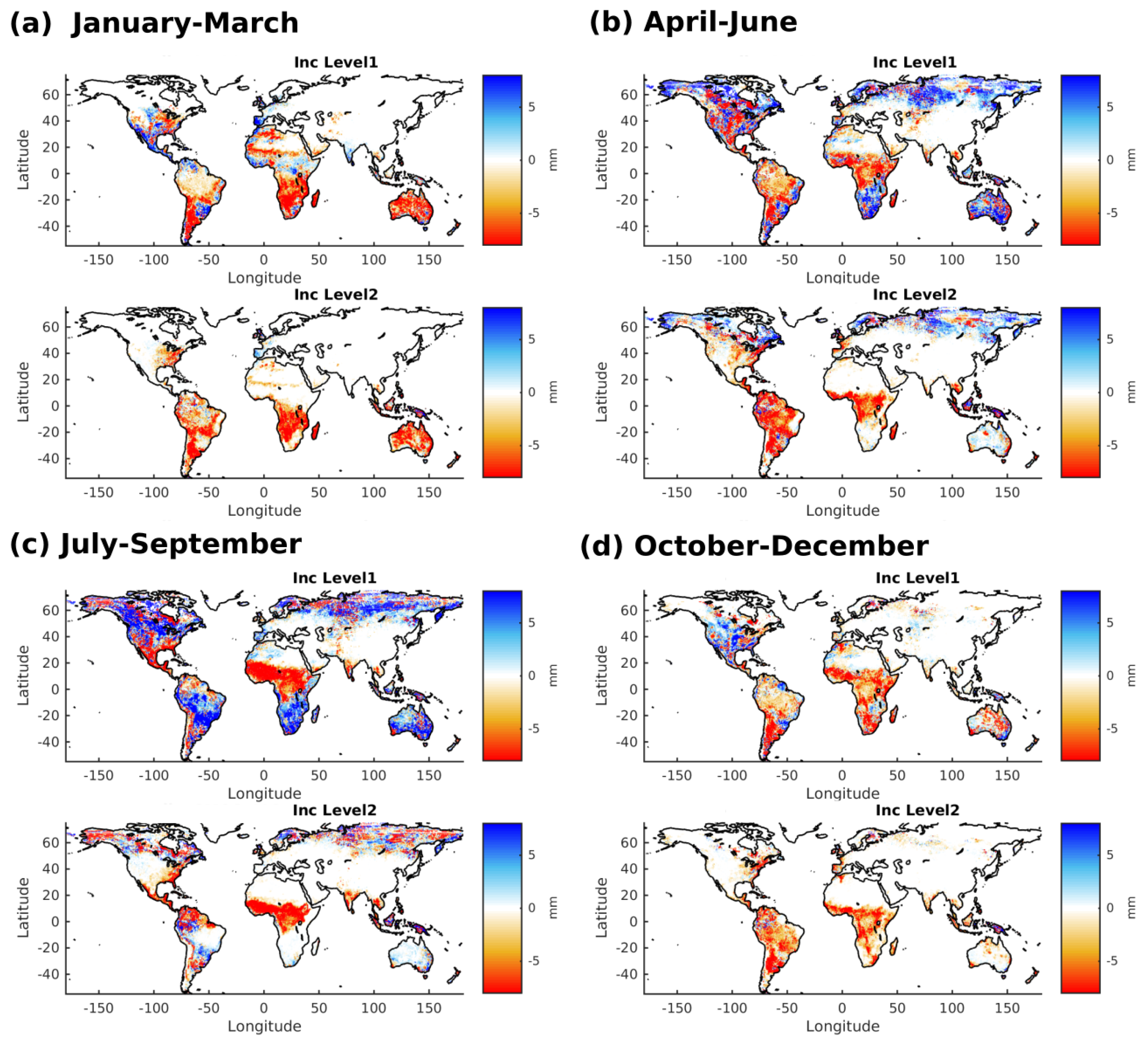
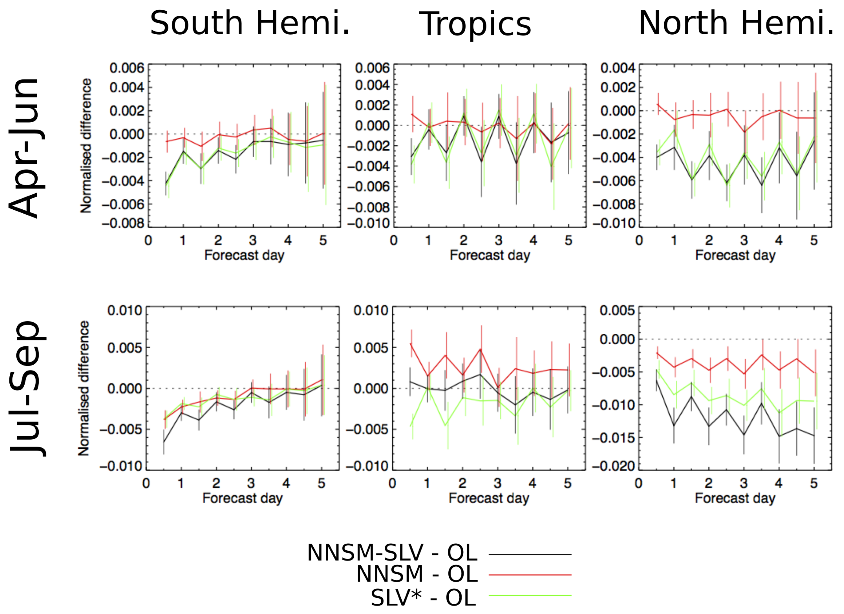
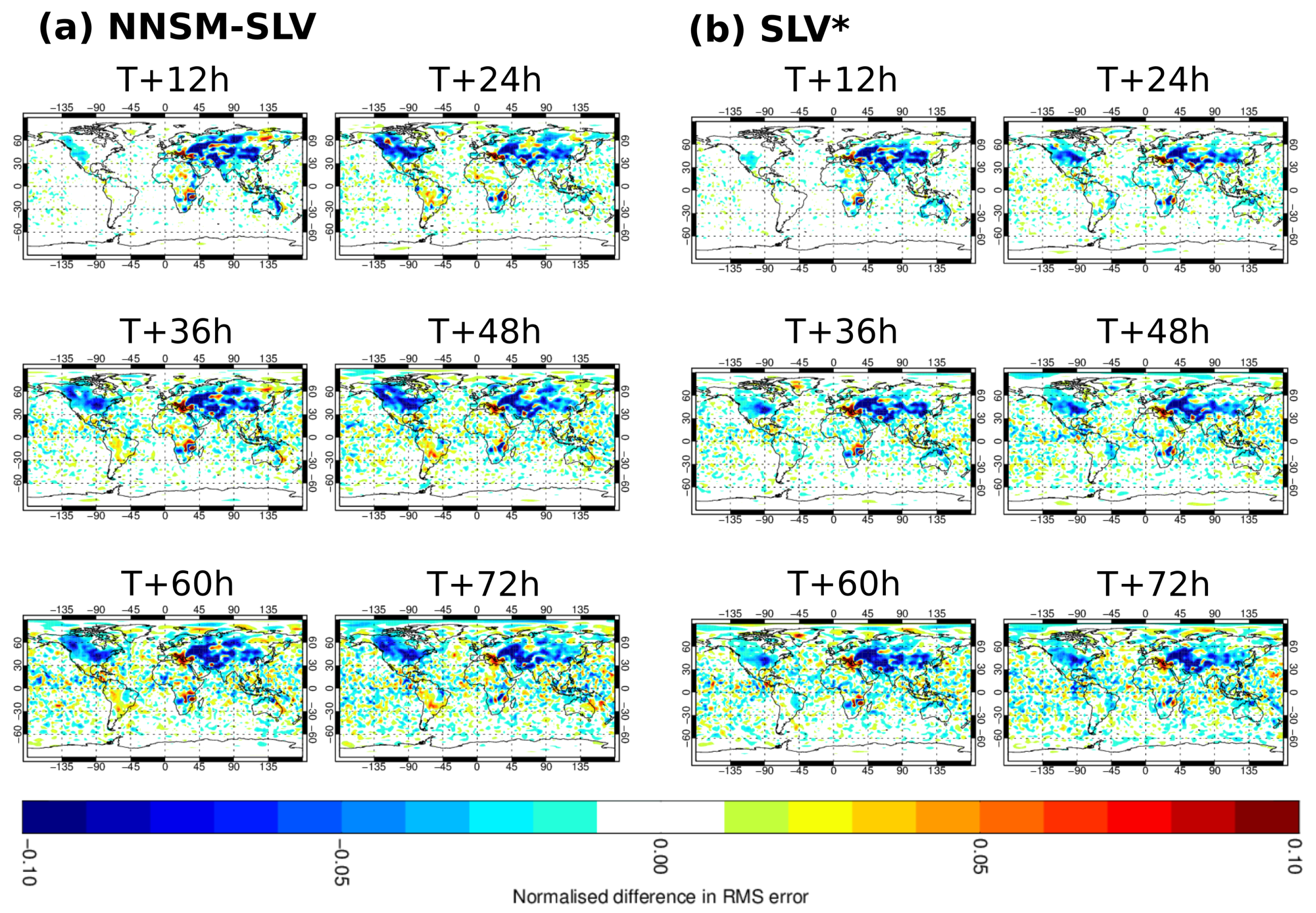
4.4. Sensitivity of the Atmosphere to the Soil Moisture Analysis

As explained in Section 3.4, the open loop and the analysed surface fields were used to compute atmospheric forecast experiments for the whole year 2012, which were evaluated with respect to the operational IFS analysis in periods of three months using several metrics as the root mean square difference (RMS) or the standard deviation (STD). The metrics obtained for the forecasts using as input the SM analysis from experiments NNSM, NNSM-SLV, NNSM${}_{LW}$ and SLV* were compared to those of the forecast using as input the SM fields with no assimilation (OL). Some of the results are shown in Figure 10 and Figure 11 as the difference in RMS for the forecasts using the analyzed SM fields (with respect the 2012 IFS analysis, see Section 3.4) minus the RMS of the forecast OL SM fields (with respect the 2012 IFS analysis). Therefore, negative scores mean that the forecast using the analysed surface fields exhibit better performance than the forecasts using the open loop. Figure 10 shows the skill to forecast T_2m as a function of the forecast day averaged in periods of three months. Similar results were found for RH_2m or for the dew point forecast. A neutral impact was found for experiment NNSM${}_{LW}$, therefore it is not shown in Figure 10.

In the tropics (20${}^{\circ }$S–20${}^{\circ }$N, middle panels of Figure 10), all experiments exhibit similar performance to the open loop, with errorbars indicating non-significant impacts. However, the experiments NNSM-SLV and SLV* show some small improvements for October–December (not shown in Figure 10). In contrast, experiment NNSM might imply a slight decrease of performance in July–September (taking into account the errorbars, the RMS difference is compatible with a neutral impact).

Left panels of Figure 10 show the results for the Southern Hemisphere extra tropics (20${}^{\circ }$S–90${}^{\circ }$S). The forecasts using SM from experiments NNSM-SLV or SLV* show an improvement for all the seasons. The improvement is higher in July–December, being significant until days 4–5 in October–December (not shown in Figure 10). When using SM from the NNSM experiment the forecast skill improve up to day 2–3 in July–September. It is noteworthy that in this period, the forecast skill when using the NNSM-SLV analysis is better than that using the SLV* analysis. In conclusion, SMOS NNSM adds significant information to the SLVs and improves the forecast in the Southern Hemisphere extra tropics mainly in the southern spring.

Right panels of Figure 10 show the results for the Northern Hemisphere extra tropics (20${}^{\circ }$N–90${}^{\circ }$N). Forecasts using NNSM-SLV and SLV* show an increase in performance in April–September (Figure 10). As in the Southern Hemisphere, the RMS decreases more for forecasts using NNSM-SLV than for those using only the SM analysis with SLV* DA. The forecast using the SM analysis from the NNSM NN DA alone also has a significant positive effect in July–September.

To get further insight into the increase in forecasts skill when using the NNSM and NNSM-SLV analyzed SM fields, it was also studied using global maps. Figure 11 shows maps of the forecast skill for air temperature at 850 hPa averaged for the July–September period as a function of the forecast time from 12 to 72 h. The six left panels (Figure 11a) show the results for experiment NNSM-SLV and the six right panels (Figure 11b) show the results for experiment SLV*. The comparison of Figure 11a,b show that NNSM-SLV improves the forecast in Canada and to a lesser extend in Northern Asia up to 72 h with respect to the SLV* analysis. Figure 4, Figure 5a and Figure 6c show that innovations and increments in those regions in summer are positive, meaning that SMOS NN SM is adding moisture to the model and this improves the atmospheric forecast for variables close to the surface such as T_2m, RH_2m or the dew point.

5. Discussion

5.1. On the Low Impact of the Soil Moisture Analysis at Locations with In Situ Measurements

As discussed in Section 4.3, even if there are significant differences from site to site, the global impact of the soil moisture analysis is low at the locations where in situ measurements are available. One must bear in mind that the ratio of observation error versus model error is in principle different for each site and it can be high in some places, giving low weight to the observations for the DA. It is also important to remark that the regions with more SM in situ measurements (North America and Europe) are also those were NWP models are the best constrained by a large number of conventional observations and the models are already very good.

Blankenship et al. [15] discussed the assimilation of SMOS SM into the Noah LSM via an Ensemble Kalman Filter within the National Aeronautics and Space Administration Land Information System. An experiment was run for the warm season of 2011 in central and southeastern United States. This experiment showed that SMOS DA significantly increased the correlation of Noah SM with station measurements from 0.45 to 0.57 in the 0–10 cm layer. However, the modest contribution of the SM DA into state-of-the-art models at the sites with in situ measurements found in this study is in agreement with previous results from other DA experiments. The first results on the assimilation of SMOS $T_{\mathrm{b}}$s observations for SM analysis at ECMWF were slightly beneficial for soil moisture analysis in a 15-days period at the location of two stations of the SCAN network, increasing the correlation from 0.72 to 0.79 [9]. As discussed above, many sites and larger time periods must be analyzed to obtain robust results. A more general result using tens of sites was discussed by Muñoz-Sabater et al. [58], who presented a one-month DA experiment over North America. They obtained correlations of 0.68, 0.64 and 0.70 against in situ measurements by the USCRN network for OL, SMOS $T_{\mathrm{b}}$s DA and SMOS $T_{\mathrm{b}}$s + SLVs DA, respectively, and 0.63, 0.61 and 0.65 against in situ measurements by the SCAN network for OL, SMOS $T_{\mathrm{b}}$s DA and SMOS $T_{\mathrm{b}}$s + SLVs DA, respectively.

Lievens et al. [59] discussed the assimilation of SMOS $T_{\mathrm{b}}$s into the GLEAM model and tested the performance to improve SM and land evaporation estimates. They compared the analyzed SM to in situ measurements over 358 sites finding a correlation of 0.65 for the OL and 0.68 for the SMOS $T_{\mathrm{b}}$s DA experiment. Similar conclusions were obtained by Kolassa et al. [60], who used NN estimates of SM computed from Soil Moisture Active Passive (SMAP) observations for DA into the National Aeronautics and Space Administration (NASA) Catchment model over the contiguous United States for April 2015 to March 2017. Assimilating the NN retrievals without further bias correction improved the correlations against in situ measurements for 14 SMAP core validation sites by 0.12, over the model-only skill and reduced the surface SM STD by 0.005 m${}^3$m${}^{-3}$. Assimilating the NN retrievals after a localized bias correction yielded slightly lower surface correlation and STD improvements. Finally, similar results were discussed by Gevaert et al. [61] studying the joint assimilation of SM retrieved from multiple passive microwave frequencies into the Australian Water Resources Assessment landscape hydrology model. L- and X-band SM improved the correlation with respect to in situ measurements by 0.11 and 0.08, while SM derived from C-band observations improved the correlation by 0.04.

The current study uses a much larger evaluation data set (more than 900 sensors) than those used in the studies cited above and, as shown in Figure 9, at some sites the correlation improves by similar (or higher) values to those found in previous studies [60,61]. In summary, the average low impact of the SM analysis at the location of in situ measurement sites is in agreement with previous studies. Of course, one must bear in mind that, even if the evaluation has been done in a large number of sites, the conclusions are not necessarily representative for the entire globe. Furthermore, in the regions where these in situ measurements have been acquired the models are already very good thanks to the large number of conventional observations that are already used for assimilation and evaluation.

5.2. On the Effect for Atmospheric Forecasts

Regarding the impact of SM or $T_{\mathrm{b}}$s data assimilation on atmospheric forecasts, there is a limited number of studies that can be used for comparison. A first study of the impact of directly assimilating SMOS $T_{\mathrm{b}}$s observations on SM analysis and the atmospheric scores near the surface was presented by Muñoz-Sabater et al. [9]. The results did not provide evidence of significant improvements of air temperature and air humidity. In a subsequent study the sensitivity to SMOS observation errors and model errors was studied further but the conclusion was that the atmospheric impact, limited to the closest layer to the surface, is minimal [58]. Muñoz-Sabater et al. [7,9] used fully coupled surface and atmosphere simulations for a one-month DA experiment over one continent. They assimilated SMOS $T_{\mathrm{b}}$s using a radiative transfer observation operator. In contrast, the current study used atmospheric forecast initialized with the analyzed surface fields but it is global and it spans a complete year. Instead of SMOS $T_{\mathrm{b}}$s, a SM dataset obtained from SMOS observations was assimilated after using an off-line NN as observation operator. The current study relies on a 24 h window DA, while the Muñoz-Sabater et al. studies [9,58] used a 12 h DA window (although it is not suitable for operational applications). The offline approach has the great advantage to enable performing, at a reasonable computing cost, the extensive set of DA experiments required for research purposes, for instance to study the relative impact of different observation types into the assimilation. In addition it makes it possible to run one-year long DA experiments, which ensures the statistical robustness of the results such as the positive impact on the atmospheric forecast discussed in Section 4.2. The offline approach used a NN to invert the SMOS observations to compute a SM data set that is, by construction, consistent with the global climatology of the model. In spite of the global consistency in the climatology and the non-existence of a global bias, local bias can be present as discussed when analyzing the innovations in Section 4. However, Kolassa et al. [60] found that an intermediate step of local bias correction after training the NN using model fields do not change significantly the results.

6. Summary and Conclusions

A set of SM DA experiments was presented and evaluated for NWP applications in order to measure the information provided by the SMOS observations. The DA experiments were carried out using the H-TESSEL land surface model and the offline so-LDAS in order to use a very computationally efficient system for long assimilation experiments (one full year here). The analysis was done for SM in the first three layers of the model by assimilating jointly SMOS SM retrievals and conventional T_2m and RH_2m. The SM retrievals were produced specifically for this study, by training a NN using SMOS brightness temperatures as input and H-TESSEL data as SM examples. This approach has several advantages: (1) the SMOS information is processed in NRT since the NN processing is very fast, (2) the SMOS retrievals share some statistical features with the model (such as global bias, or similar climatology) to facilitate their assimilation without any CDF-matching that can distort the satellite spatial information towards the model patterns, and (3) to avoid the use of a surface radiative transfer that is still difficult to model and for which it is difficult to provide state-dependent uncertainties.

The different SM analyses were studied and compared for the four quarters of 2012. Some seasonal effects and regional differences were found when using SMOS NNSM. For instance cumulative increments for experiments using NNSM in Australia, South Africa and parts of South America are negative in October-March, but they are positive from April to September. The increments in the first soil layer due to the assimilation of T_2m and RH_2m are significant in the west of North America, central Asia, the Sahel, South Africa, part of the Amazon region, and Australia. Furthermore, the SLVs complement well the SMOS SM observations by better constraining the SM content of deeper soil layers.

The different SM analyzed fields were evaluated against a large number of in situ SM measurements. Significant differences were found from site to site but on average the SM analysis gives similar results to the model open loop for the sites with in situ measurements. This is in agreement with previous results in the literature, and can be understood since the models are already constrained by many conventional observations on these locations. However, in the current study, the different DA experiments where also evaluated by using the analysed SM fields to initialise atmospheric forecasting experiments, to assess their impact on NWP performance. NNSM data assimilation may slightly degrade the forecast in the Tropics in July–September. However, all experiments using jointly NNSM and SLVs improve the forecast for all the seasons in the Southern hemisphere, where conventional observations are lacking. The NNSM-only DA also improves the forecast in July–September. Finally, in the Northern Hemisphere, the experiments with NNSM and SLVs improve the forecast in April–September. NNSM-only DA also improves the forecast in July–September. Maps of the forecasting skill with respect to the open loop experiment show that SMOS NNSM improves the forecast in North America and to a lesser extend in Northern Asia for up to 72 h.

In conclusion, an innovative technique that uses a NN to retrieve a SMOS SM consistent with the model (by construction) prior to the assimilation was discussed and evaluated. The results obtained for the assimilation of SMOS NNSM are promising as they show a positive impact in the forecast. The low computational cost of the offline NN SM retrieval with respect to an online approximative radiative transfer observation operator and the promising results have triggered a strong interest for operational applications.

References

1. Koster, R.D.; Dirmeyer, P.A.; Guo, Z.; Bonan, G.; Chan, E.; Cox, P.; Gordon, C.T.; Kanae, S.; Kowalczyk, E.; Lawrence, D.; et al. Regions of strong coupling between soil moisture and precipitation. Science 2004, 305, 1138–1140. [Google Scholar] [CrossRef] [PubMed]
2. Tuttle, S.; Salvucci, G. Empirical evidence of contrasting soil moisture–precipitation feedbacks across the United States. Science 2016, 352, 825–828. [Google Scholar] [CrossRef] [PubMed]
3. Seneviratne, S.I.; Corti, T.; Davin, E.L.; Hirschi, M.; Jaeger, E.B.; Lehner, I.; Orlowsky, B.; Teuling, A.J. Investigating soil moisture–climate interactions in a changing climate: A review. Earth-Sci. Rev. 2010, 99, 125–161. [Google Scholar] [CrossRef]
4. Parrens, M.; Mahfouf, J.F.; Barbu, A.; Calvet, J.C. Assimilation of surface soil moisture into a multilayer soil model: design and evaluation at local scale. Hydrol. Earth Syst. Sci. 2014, 18, 673–689. [Google Scholar] [CrossRef] [Green Version]
5. De Lannoy, G.J.; Reichle, R.H. Global Assimilation of Multiangle and Multipolarization SMOS Brightness Temperature Observations into the GEOS-5 Catchment Land Surface Model for Soil Moisture Estimation. J. Hydrometeorol. 2016, 17, 669–691. [Google Scholar] [CrossRef] [Green Version]
6. Lievens, H.; Lannoy, G.D.; Bitar, A.A.; Drusch, M.; Dumedah, G.; Franssen, H.J.H.; Kerr, Y.; Tomer, S.; Martens, B.; Merlin, O.; et al. Assimilation of SMOS soil moisture and brightness temperature products into a land surface model. Remote Sens. Environ. 2016, 180, 292–304. [Google Scholar] [CrossRef]
7. Muñoz Sabater, J.; Lawrence, H.; Albergel, C.; de Rosnay, P.; Isaken, L.; Mecklenburg, S.; Kerr, Y.; Drusch, M. Assimilation of SMOS Brightness Temperatures in the ECMWF Integrated Forecasting System. QJRMS 2019, in press. [Google Scholar]
8. Kerr, Y.; Waldteufel, P.; Wigneron, J.P.; Delwart, S.; Cabot, F.; Boutin, J.; Escorihuela, M.J.; Font, J.; Reul, N.; Gruhier, C.; et al. The SMOS Mission: New Tool for Monitoring Key Elements ofthe Global Water Cycle. Proc. IEEE 2010, 98, 666–687. [Google Scholar] [CrossRef] [Green Version]
9. Muñoz-Sabater, J. Incorporation of passive microwave Brightness Temperatures in the ECMWF soil moisture analysis. Remote Sens. 2015, 7, 5758–5784. [Google Scholar] [CrossRef]
10. De Rosnay, P.; Muñoz Sabater, J.; Albergel, C.; Isaken, L.; English, S.; Drusch, M.; Wigneron, J. SMOS brightness temperature forward modelling and long term monitoring at ECMWF. RSE 2019. submitted. [Google Scholar]
11. Aires, F.; Prigent, C.; Buehler, S.A.; Eriksson, P.; Milz, M.; Crewell, S. Towards more realistic hypotheses for the information content analysis of cloudy/precipitating situations–Application to a hyperspectral instrument in the microwave. Q. J. R. Meteorol. Soc. 2019, 145, 1–14. [Google Scholar] [CrossRef]
12. Rodríguez-Fernández, N.J.; Muñoz-Sabater, J.; Richaume, P.; Albergel, C.; de Rosnay, P.; Kerr, Y.H.; Drusch, M.; Mecklenburg, S. SMOS near real time soil moisture product: Processor overview and first validation results. Hydrol. Earth Syst. Sci. 2017, 21, 5201–5216. [Google Scholar] [CrossRef]
13. Xu, X.; Tolson, B.A.; Li, J.; Staebler, R.M.; Seglenieks, F.; Haghnegahdar, A.; Davison, B. Assimilation of SMOS soil moisture over the Great Lakes basin. Remote Sens. Environ. 2015, 169, 163–175. [Google Scholar] [CrossRef]
14. Leroux, D.J.; Pellarin, T.; Vischel, T.; Cohard, J.M.; Gascon, T.; Gibon, F.; Mialon, A.; Galle, S.; Peugeot, C.; Seguis, L. Assimilation of SMOS soil moisture into a distributed hydrological model and impacts on the water cycle variables over the Ouémé catchment in Benin. Hydrol. Earth Syst. Sci. 2016, 20, 2827–2840. [Google Scholar] [CrossRef]
15. Blankenship, C.B.; Case, J.L.; Zavodsky, B.T.; Crosson, W.L. Assimilation of SMOS Retrievals in the Land Information System. IEEE Trans. Geosci. Remote Sens. 2016, 54, 6320–6332. [Google Scholar] [CrossRef] [PubMed] [Green Version]
16. Martens, B.; Miralles, D.; Lievens, H.; Fernández-Prieto, D.; Verhoest, N. Improving terrestrial evaporation estimates over continental Australia through assimilation of SMOS soil moisture. Int. J. Appl. Earth Obs. Geoinf. 2016, 48, 146–162. [Google Scholar] [CrossRef]
17. Ridler, M.E.; Madsen, H.; Stisen, S.; Bircher, S.; Fensholt, R. Assimilation of SMOS-derived soil moisture in a fully integrated hydrological and soil-vegetation-atmosphere transfer model in Western Denmark. Water Resour. Res. 2014, 50, 8962–8981. [Google Scholar] [CrossRef]
18. Scholze, M.; Kaminski, T.; Knorr, W.; Blessing, S.; Vossbeck, M.; Grant, J.; Scipal, K. Simultaneous assimilation of SMOS soil moisture and atmospheric CO2 in-situ observations to constrain the global terrestrial carbon cycle. Remote Sens. Environ. 2016, 180, 334–345. [Google Scholar] [CrossRef]
19. Drusch, M.; Wood, E.; Gao, H. Observation operators for the direct assimilation of TRMM microwave imager retrieved soil moisture. Geophys. Res. Lett. 2005, 32. [Google Scholar] [CrossRef]
20. De Rosnay, P.; Drusch, M.; Vasiljevic, D.; Balsamo, G.; Albergel, C.; Isaksen, L. A simplified Extended Kalman Filter for the global operational soil moisture analysis at ECMWF. Q. J. R. Meteorol. Soc. 2013, 139, 1199–1213. [Google Scholar] [CrossRef]
21. Aires, F.; Prigent, C.; Rossow, W.B. Sensitivity of satellite microwave and infrared observations to soil moisture at a global scale: 2. Global statistical relationships. J. Geophys. Res. 2005, 110. [Google Scholar] [CrossRef] [Green Version]
22. Aires, F.; Prigent, C. Toward a new generation of satellite surface products? J. Geophys. Res. Atmos. (1984–2012) 2006, 111. [Google Scholar] [CrossRef] [Green Version]
23. Rodríguez-Fernández, N.J.; Aires, F.; Richaume, P.; Kerr, Y.H.; Prigent, C.; Kolassa, J.; Cabot, F.; Jiménez, C.; Mahmoodi, A.; Drusch, M. Soil moisture retrieval using neural networks: Application to SMOS. IEEE Trans. Geosci. Remote Sens. 2015, 53, 5991–6007. [Google Scholar] [CrossRef]
24. Jiménez, C.; Clark, D.B.; Kolassa, J.; Aires, F.; Prigent, C. A joint analysis of modeled soil moisture fields and satellite observations. J. Geophys. Res. Atmos. 2013, 118, 6771–6782. [Google Scholar] [CrossRef] [Green Version]
25. Seuffert, G.; Wilker, H.; Viterbo, P.; Drusch, M.; Mahfouf, J. The usage of screen-level parameters and microwave brightness temperature for soil moisture analysis. J. Hydrometeorol. 2004, 5, 516–531. [Google Scholar] [CrossRef]
26. Kalnay, E. Atmospheric Modeling, Data Assimilation and Predictability; Cambridge University Press: Cambridge, UK, 2002. [Google Scholar] [CrossRef]
27. Mahfouf, J.F. Analysis of soil moisture from near-surface parameters: A feasibility study. J. Appl. Meteorol. 1991, 30, 1534–1547. [Google Scholar] [CrossRef]
28. Douville, H.; Viterbo, P.; Mahfouf, J.F.; Beljaars, A.C. Evaluation of the optimum interpolation and nudging techniques for soil moisture analysis using FIFE data. Mon. Weather Rev. 2000, 128, 1733–1756. [Google Scholar] [CrossRef]
29. Balsamo, G.; Bouyssel, F.; Noilhan, J. A simplified bi-dimensional variational analysis of soil moisture from screen-level observations in a mesoscale numerical weather-prediction model. Q. J. R. Meteorol. Soc. 2004, 130, 895–915. [Google Scholar] [CrossRef]
30. Mahfouf, J.F.; Bergaoui, K.; Draper, C.; Bouyssel, F.; Taillefer, F.; Taseva, L. A comparison of two off-line soil analysis schemes for assimilation of screen level observations. J. Geophys. Res. Atmos. 2009, 114. [Google Scholar] [CrossRef]
31. Balsamo, G.; Mahfouf, J.; Bélair, S.; Deblonde, G. A land data assimilation system for soil moisture and temperature: An information content study. J. Hydrometeorol. 2007, 8, 1225–1242. [Google Scholar] [CrossRef]
32. Drusch, M.; Scipal, K.; De Rosnay, P.; Balsamo, G.; Andersson, E.; Bougeault, P.; Viterbo, P. Towards a Kalman Filter based soil moisture analysis system for the operational ECMWF Integrated Forecast System. Geophys. Res. Lett. 2009, 36. [Google Scholar] [CrossRef]
33. Drusch, M. Initializing numerical weather prediction models with satellite-derived surface soil moisture: Data assimilation experiments with ECMWF’s Integrated Forecast System and the TMI soil moisture data set. J. Geophys. Res. Atmos. (1984–2012) 2007, 112. [Google Scholar] [CrossRef]
34. Scipal, K.; Drusch, M.; Wagner, W. Assimilation of a ERS scatterometer derived soil moisture index in the ECMWF numerical weather prediction system. Adv. Water Resour. 2008, 31, 1101–1112. [Google Scholar] [CrossRef]
35. Al Bitar, A.; Mialon, A.; Kerr, Y.; Cabot, F.; Richaume, P.; Jacquette, E.; Quesney, A.; Mahmoodi, A.; Tarot, S.; Parrens, M.; et al. The Global SMOS Level 3 daily soil moisture and brightness temperature maps. Earth Syst. Sci. Data 2017, 9, 293–315. [Google Scholar] [CrossRef]
36. Brodzik, M.J.; Billingsley, B.; Haran, T.; Raup, B.; Savoie, M.H. EASE-Grid 2.0: Incremental but Significant Improvements for Earth-Gridded Data Sets. ISPRS Int. J. Geo-Inf. 2012, 1, 32–45. [Google Scholar] [CrossRef] [Green Version]
37. Balsamo, G.; Beljaars, A.; Scipal, K.; Viterbo, P.; van den Hurk, B.; Hirschi, M.; Betts, A.K. A revised hydrology for the ECMWF model: Verification from field site to terrestrial water storage and impact in the Integrated Forecast System. J. Hydrometeorol. 2009, 10, 623–643. [Google Scholar] [CrossRef]
38. Balsamo, G.; Dutra, E.; Boussetta, S.; Beljaars, A.; Viterbo, P.; van den Hurk, B. Recent advances in land surface modelling at ECMWF. In Proceedings of the ECMWF/GLASS workshop on Land Surface Modelling, Reading, UK, 9–12 November 2009; pp. 9–12. [Google Scholar]
39. Albergel, C.; Balsamo, G.; Rosnay, P.d.; Muñoz-Sabater, J.; Boussetta, S. A bare ground evaporation revision in the ECMWF land-surface scheme: Evaluation of its impact using ground soil moisture and satellite microwave data. Hydrol. Earth Syst. Sci. 2012, 16, 3607–3620. [Google Scholar] [CrossRef]
40. Boussetta, S.; Balsamo, G.; Beljaars, A.; Kral, T.; Jarlan, L. Impact of a satellite-derived leaf area index monthly climatology in a global numerical weather prediction model. Int. J. Remote Sens. 2013, 34, 3520–3542. [Google Scholar] [CrossRef]
41. Balsamo, G.; Albergel, C.; Beljaars, A.; Boussetta, S.; Brun, E.; Cloke, H.; Dee, D.; Dutra, E.; Muñoz-Sabater, J.; Pappenberger, F.; et al. ERA-Interim/Land: A global land surface reanalysis data set. Hydrol. Earth Syst. Sci. 2015, 19, 389–407. [Google Scholar] [CrossRef]
42. Dee, D.; Uppala, S.; Simmons, A.; Berrisford, P.; Poli, P.; Kobayashi, S.; Andrae, U.; Balmaseda, M.; Balsamo, G.; Bauer, P.; et al. The ERA-Interim reanalysis: Configuration and performance of the data assimilation system. Q. J. R. Meteorol. Soc. 2011, 137, 553–597. [Google Scholar] [CrossRef]
43. De Rosnay, P.; Balsamo, G.; Albergel, C.; Muñoz-Sabater, J.; Isaksen, L. Initialisation of land surface variables for numerical weather prediction. Surv. Geophys. 2014, 35, 607–621. [Google Scholar] [CrossRef]
44. Dorigo, W.; Wagner, W.; Hohensinn, R.; Hahn, S.; Paulik, C.; Xaver, A.; Gruber, A.; Drusch, M.; Mecklenburg, S.; Oevelen, P.v.; et al. The International Soil Moisture Network: A data hosting facility for global in situ soil moisture measurements. Hydrol. Earth Syst. Sci. 2011, 15, 1675–1698. [Google Scholar] [CrossRef]
45. Tagesson, T.; Fensholt, R.; Guiro, I.; Rasmussen, M.O.; Huber, S.; Mbow, C.; Garcia, M.; Horion, S.; Sandholt, I.; Holm-Rasmussen, B.; et al. Ecosystem properties of semiarid savanna grassland in West Africa and its relationship with environmental variability. Glob. Chang. Biol. 2015, 21, 250–264. [Google Scholar] [CrossRef] [PubMed]
46. Martínez-Fernández, J.; Ceballos, A. Mean soil moisture estimation using temporal stability analysis. J. Hydrol. 2005, 312, 28–38. [Google Scholar] [CrossRef]
47. Calvet, J.C.; Fritz, N.; Froissard, F.; Suquia, D.; Petitpa, A.; Piguet, B. In situ soil moisture observations for the CAL/VAL of SMOS: The SMOSMANIA network. In Proceedings of the IGARSS 2007 Geoscience and Remote Sensing Symposium, Barcelona, Spain, 23–27 July 2007; pp. 1196–1199. [Google Scholar]
48. Bircher, S.; Skou, N.; Jensen, K.H.; Walker, J.P.; Rasmussen, L. A soil moisture and temperature network for SMOS validation in Western Denmark. Hydrol. Earth Syst. Sci. 2012, 16, 1445–1463. [Google Scholar] [CrossRef] [Green Version]
49. Morbidelli, R.; Saltalippi, C.; Flammini, A.; Rossi, E.; Corradini, C. Soil water content vertical profiles under natural conditions: Matching of experiments and simulations by a conceptual model. Hydrol. Process. 2014, 28, 4732–4742. [Google Scholar] [CrossRef]
50. Schaefer, G.; Cosh, M.; Jackson, T. The USDA natural resources conservation service soil climate analysis network (SCAN). J. Atmos. Ocean. Technol. 2007, 24, 2073–2077. [Google Scholar] [CrossRef]
51. Leavesley, G.; David, O.; Garen, D.; Lea, J.; Marron, J.; Pagano, T.; Perkins, T.; Strobel, M. A modeling framework for improved agricultural water supply forecasting. In Proceedings of the AGU Fall Meeting Abstracts, San Francisco, CA, USA, 15–19 December 2008; Volume 1, p. 0497. [Google Scholar]
52. Bell, J.; Palecki, M.; Baker, C.; Collins, W.; Lawrimore, J.; Leeper, R.; Hall, M.; Kochendorfer, J.; Meyers, T.; Wilson, T.; et al. U.S. Climate Reference Network soil moisture and temperature observations. J. Hydrometeorol. 2013, 14, 977–988. [Google Scholar] [CrossRef]
53. Larson, K.M.; Small, E.E.; Gutmann, E.D.; Bilich, A.L.; Braun, J.J.; Zavorotny, V.U. Use of GPS receivers as a soil moisture network for water cycle studies. Geophys. Res. Lett. 2008, 35. [Google Scholar] [CrossRef] [Green Version]
54. Yang, K.; Qin, J.; Zhao, L.; Chen, Y.; Tang, W.; Han, M.; Chen, Z.; Lv, N.; Ding, B.; Wu, H.; et al. A multiscale soil moisture and freeze–thaw monitoring network on the third pole. Bull. Am. Meteorol. Soc. 2013, 94, 1907–1916. [Google Scholar] [CrossRef]
55. Moré, J.J. The Levenberg-Marquardt algorithm: Implementation and theory. In Numerical Analysis; Springer: Berlin/Heidelberg, Germany, 1978; pp. 105–116. [Google Scholar] [Green Version]
56. Noilhan, J.; Mahfouf, J.F. The ISBA land surface parameterisation scheme. Glob. Planet Chang. 1996, 14, 145–159. [Google Scholar] [CrossRef]
57. De Lannoy, G.J.M.; de Rosnay, P.; Reichle, R. Soil Moisture Data Assimilation; Springer: New York, NY, USA, 2016. [Google Scholar]
58. Muñoz-Sabater, J.; de Rosnay, P.; Albergel, C.; Isaksen, L. Sensitivity of soil moisture analyses to contrasting background and observation error scenarios. Water 2018, 10, 890. [Google Scholar] [CrossRef]
59. Lievens, H.; Martens, B.; Verhoest, N.; Hahn, S.; Reichle, R.; Miralles, D. Assimilation of global radar backscatter and radiometer brightness temperature observations to improve soil moisture and land evaporation estimates. Remote Sens. Environ. 2017, 189, 194–210. [Google Scholar] [CrossRef]
60. Kolassa, J.; Reichle, R.H.; Liu, Q.; Cosh, M.; Bosch, D.D.; Caldwell, T.G.; Colliander, A.; Holifield Collins, C.; Jackson, T.J.; Livingston, S.J.; et al. Data assimilation to extract soil moisture information from SMAP observations. Remote Sens. 2017, 9, 1179. [Google Scholar] [CrossRef]
61. Gevaert, A.I.; Renzullo, L.J.; Van Dijk, A.I.; Woerd, H.J.; Weerts, A.H.; De Jeu, R.A. Joint assimilation of soil moisture retrieved from multiple passive microwave frequencies increases robustness of soil moisture state estimation. Hydrol. Earth Syst. Sci. 2018, 22, 4605–4619. [Google Scholar] [CrossRef] [Green Version]
Figure 1. Flow chart of the neural network data assimilation and evaluation methodology.
Remotesensing 11 01334 g001
Figure 2. (Upper left): SMOS NNSM for day 4 June 2012. (Lower left): SMOS NNSM observation error. (Upper right): model background for the same day and first layer (ECMWF SM 1 ). (Lower right): Model background error (5% of the water holding capacity). Units are m 3 /m 3 .
Remotesensing 11 01334 g002
Figure 3. Scatter plot of the SM estimated from the NN for the test sub set with respect to the reference ECMWF SM 1 data set.
Remotesensing 11 01334 g003
Figure 4. Mean innovations (observation minus model for NNSM and RH2m and model minus observation for T2m) for two periods of three months.
Remotesensing 11 01334 g004
Figure 5. Increments sum in mm for the period July-September for experiments NNSM and NNSM L W (panels a and b) and for experiments NNSM-SLV and SLV* (panels c and d).
Remotesensing 11 01334 g005
Figure 6. Increments for the upper two model layers for experiment NNSM. (a) Sum of the increments from January to March. (b) Sum of the increments from April to June. (c) Sum of the increments from July to September. (d) Sum of the increments from October to December.
Remotesensing 11 01334 g006
Figure 7. Box plots for the STDD, the Pearson correlation R, and the bias of different experiments with respect to in situ measurements network by network. On each box, the central mark indicates the median, and the bottom and top edges of the box indicate the 25th ( q 25 ) and 75th ( q 75 ) percentiles, respectively. Points are considered as outliers if they are greater than q 75 + 1 . 5 × ( q 75 q 25 ) or less than q 25 1 . 5 × ( q 75 q 25 ) . The whiskers extend to the most extreme data points not considered outliers.
Remotesensing 11 01334 g007
Figure 8. Same as Figure 7 for networks located in North America.
Remotesensing 11 01334 g008
Figure 9. (Upper) difference of the Pearson correlation of NNSM experiment time series with respect to in situ measurements and the Pearson correlation of OL experiment time series with respect to in situ measurements. (Lower) difference of the RMS of NNSM experiment time series with respect to in situ measurements and RMS of OL experiment time series with respect to in situ measurements. In both cases, blue points show that the analysed time series are closer to the in situ measurement (higher correlation and lower RMS).
Remotesensing 11 01334 g009
Figure 10. Evaluation of the atmospheric forecast skill. The plots show the RMSE of the T2m forecast for the assimilation experiments minus the RMSE for the OL experiment as a function of the forecast day in two periods: April–June (upper panels) and July–September (lower panels). The results are shown for three latitude ranges: [−90°, −20°] (left panels), [−20°, 20°] (middle panels), [20°, 90°] (right panels).
Remotesensing 11 01334 g010
Figure 11. Evaluation on the forecast skill for air temperature at 850 hPa as a function of time (from 12 to 72 h). Average over July–September of the RMS difference of NNSM-SLV (a) and SLV (b) with respect to the open loop (negative values, blue colors, indicate an improvement of the forecast skills).
Remotesensing 11 01334 g011