Statistical Stability and Spatial Instability in Mapping Forest Tree Species by Comparing 9 Years of Satellite Image Time Series

 , , , and
Abstract
:
1. Introduction
2. Material
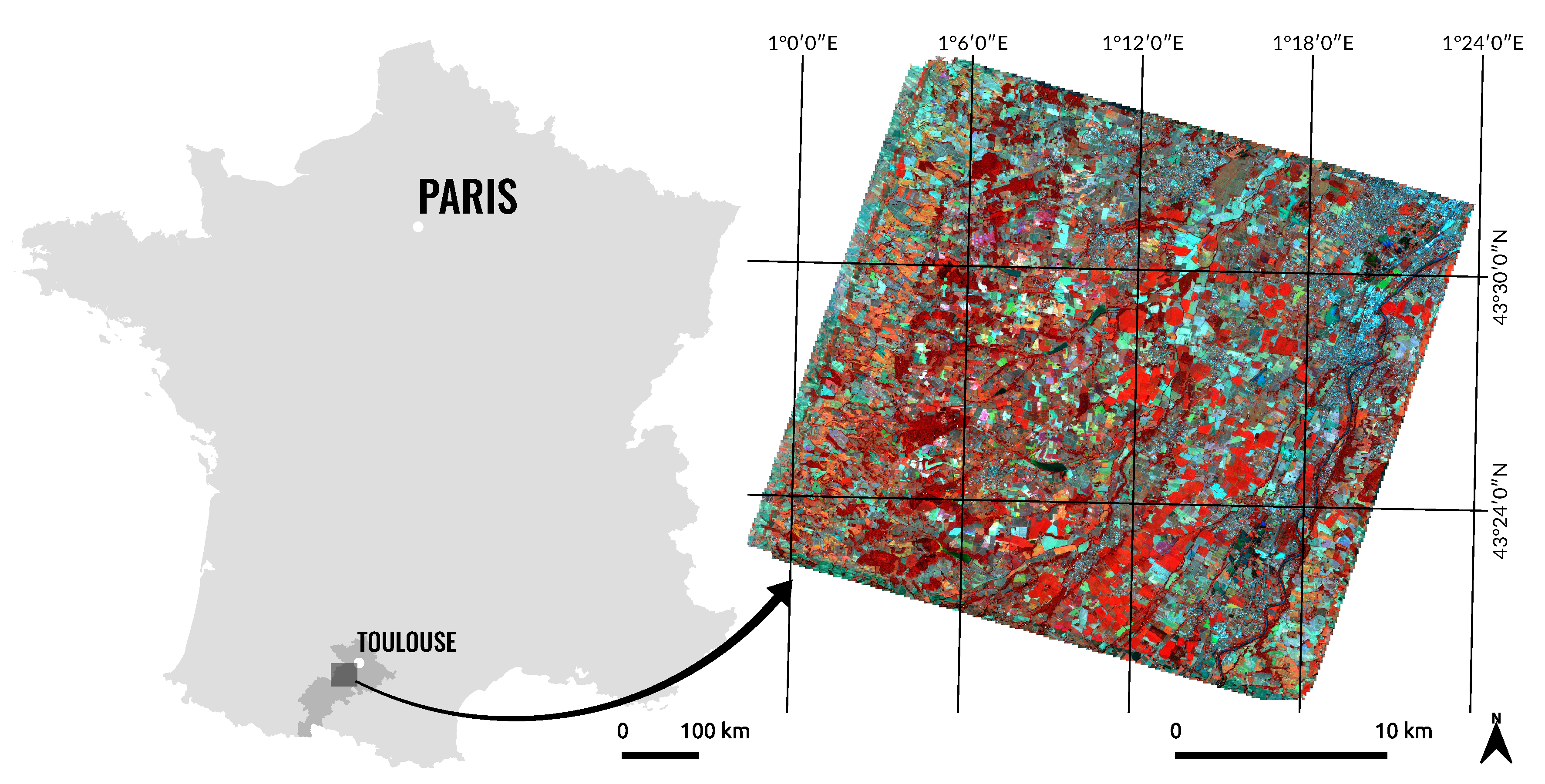
2.1. Study Area
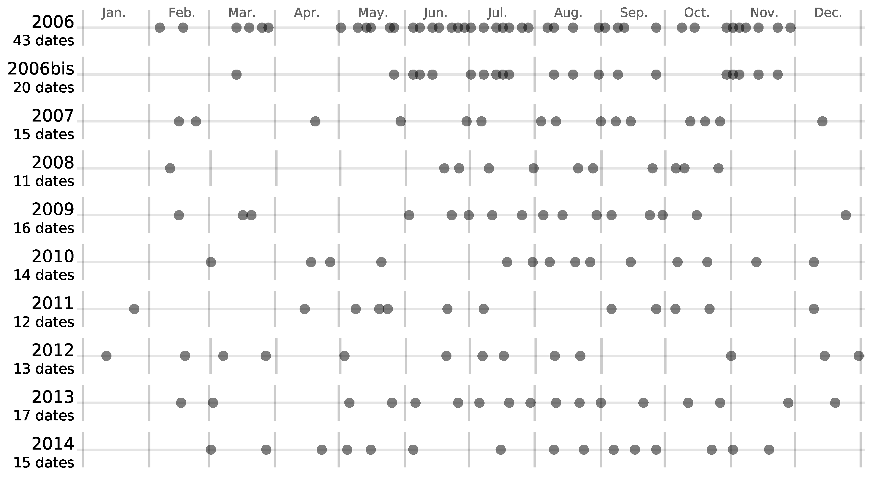
2.2. Satellite Image Time Series
2.3. Ancillary Data
2.4. Field Data
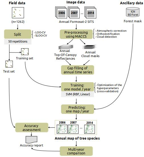
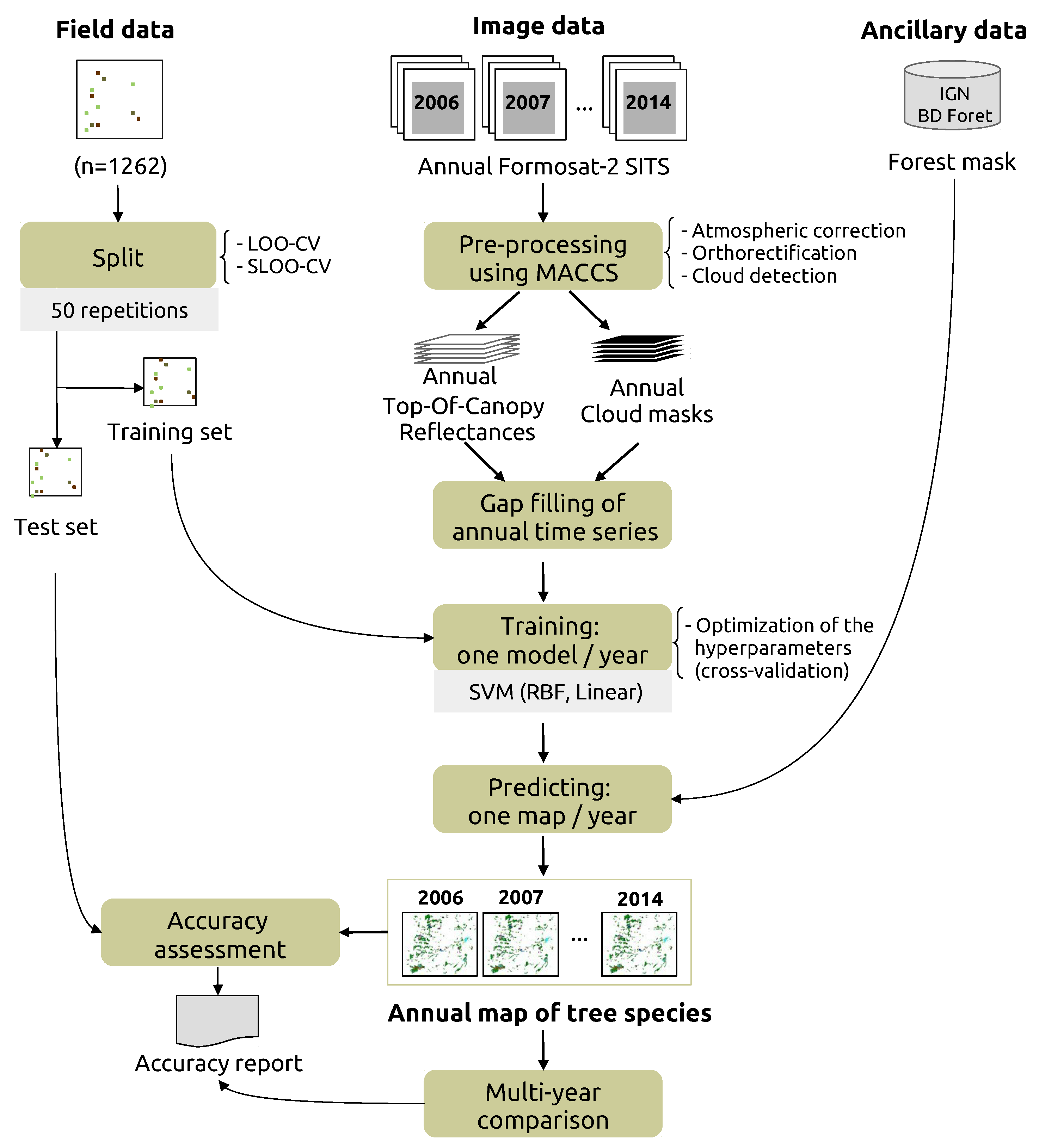
3. Classification Protocol
3.1. Pre-Processing
3.2. Training
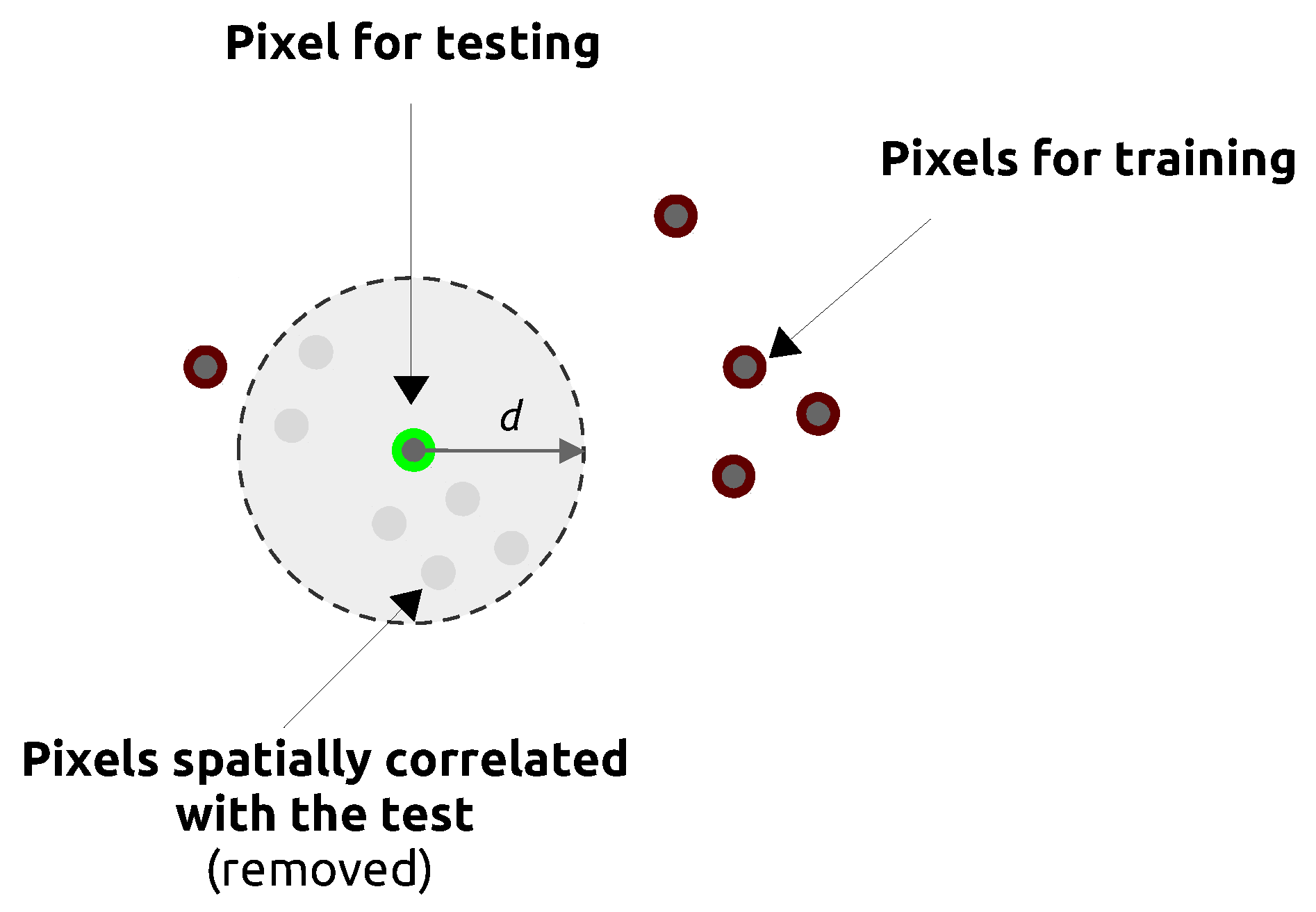
3.3. Estimating Prediction Errors by Spatial Cross-Validation
3.4. Accuracy Assessment of One-Year Classifications and Comparison
4. Results
4.1. Overall Statistical Performances
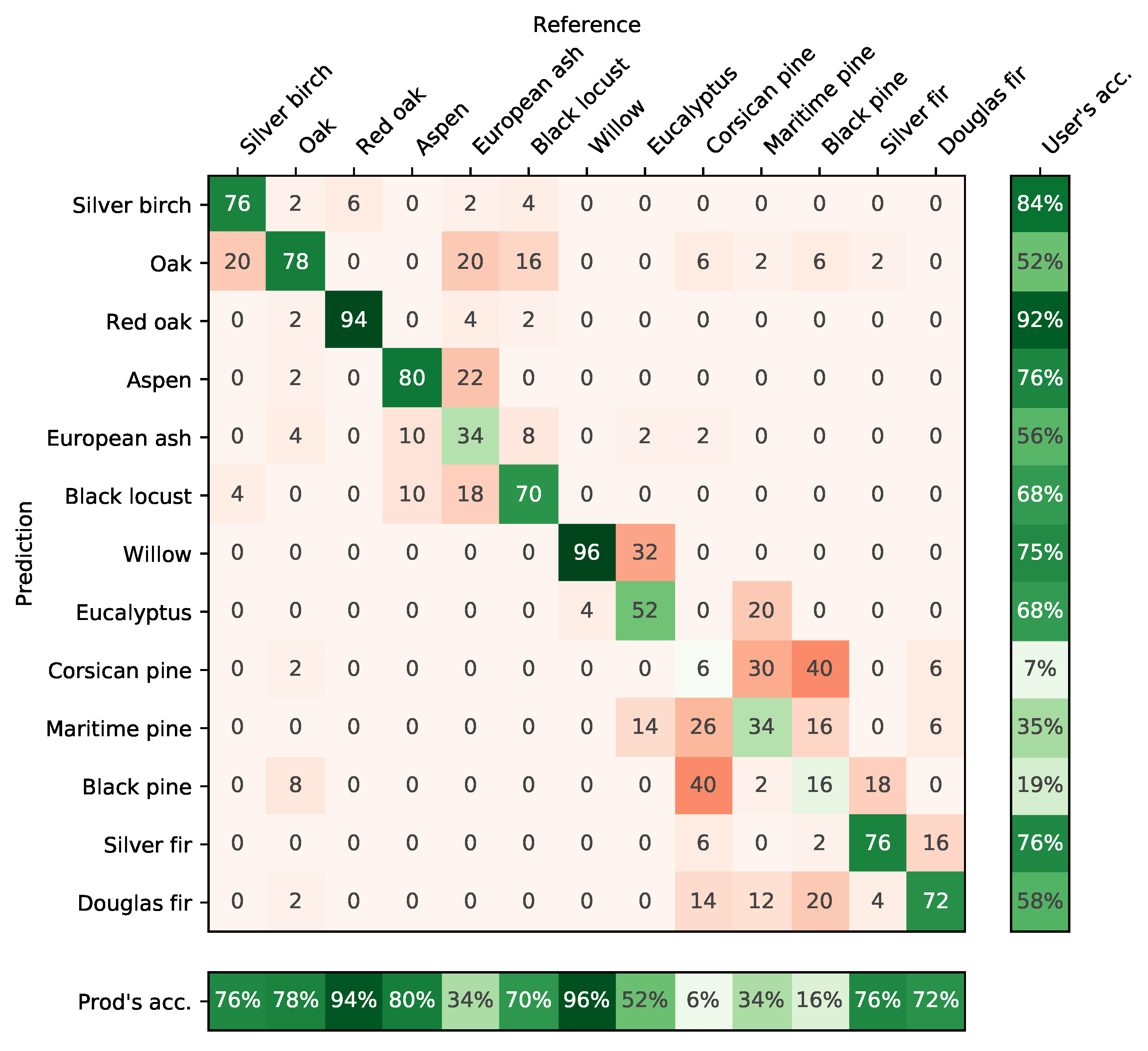
4.2. Accuracy per Species
4.3. Confusion between Species
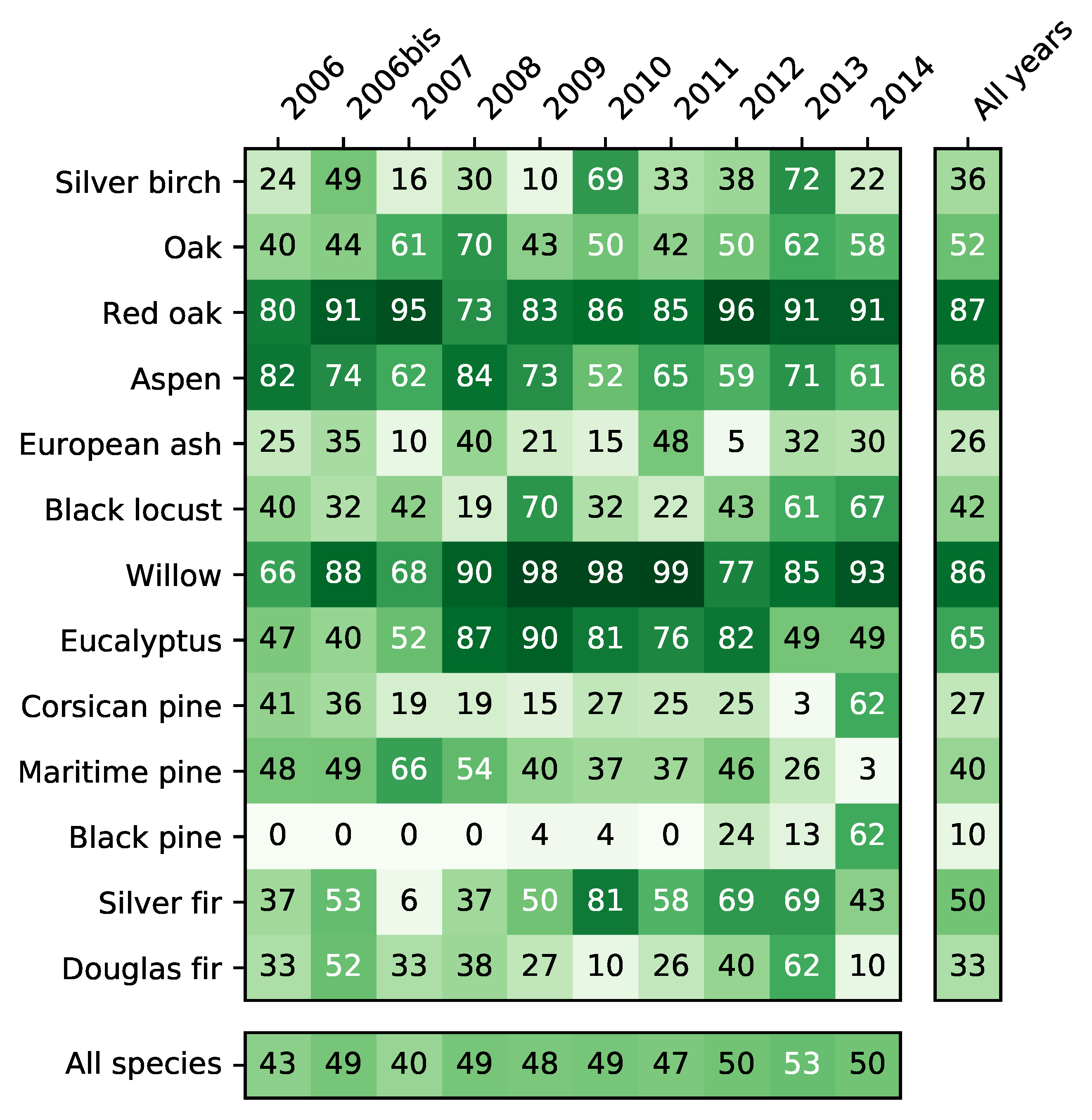
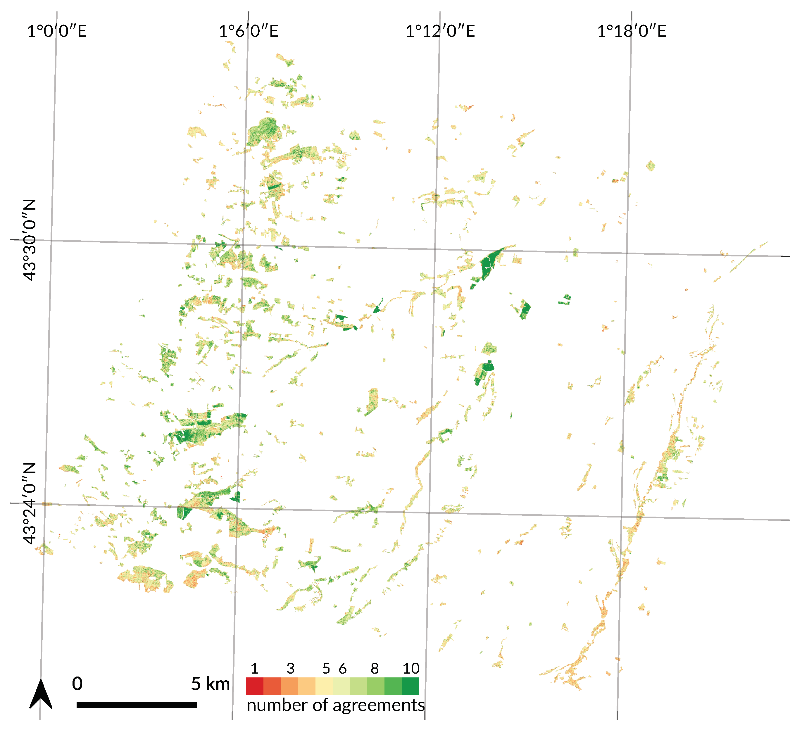
4.4. Spatial Agreement between Years
5. Discussion
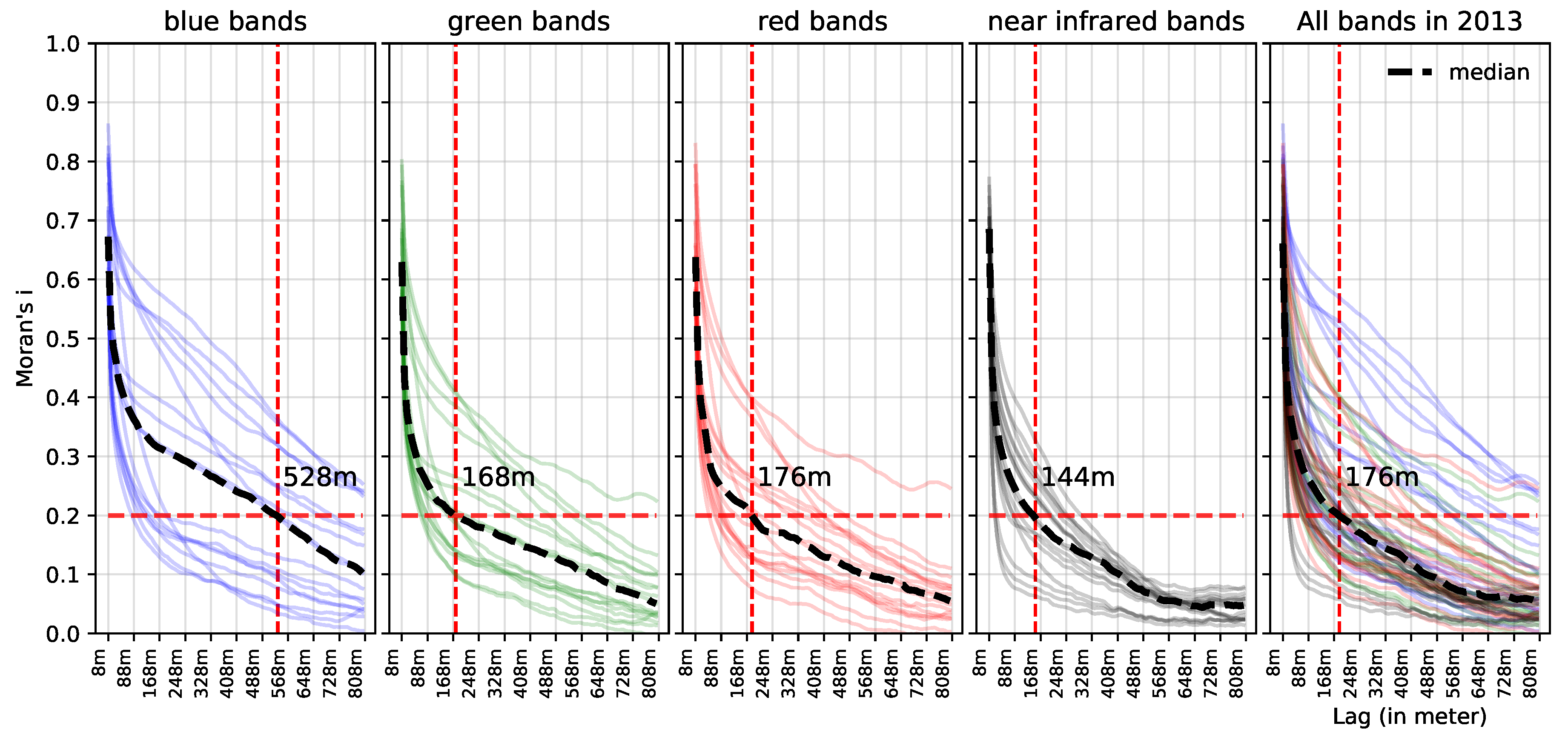
5.1. Effect of Spatial Autocorrelation: The SLOO-CV Strategy as a Standard
5.2. Effect of the Size of the Reference Sample
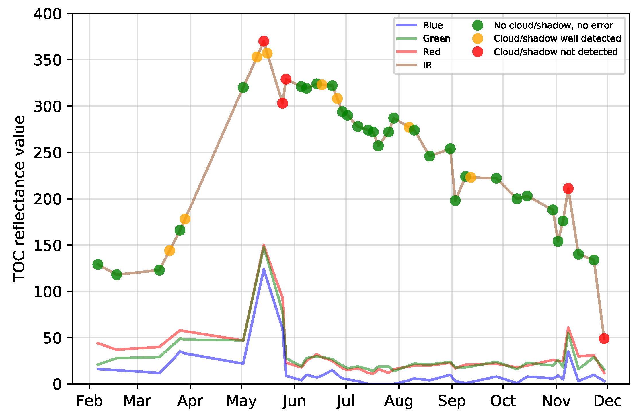
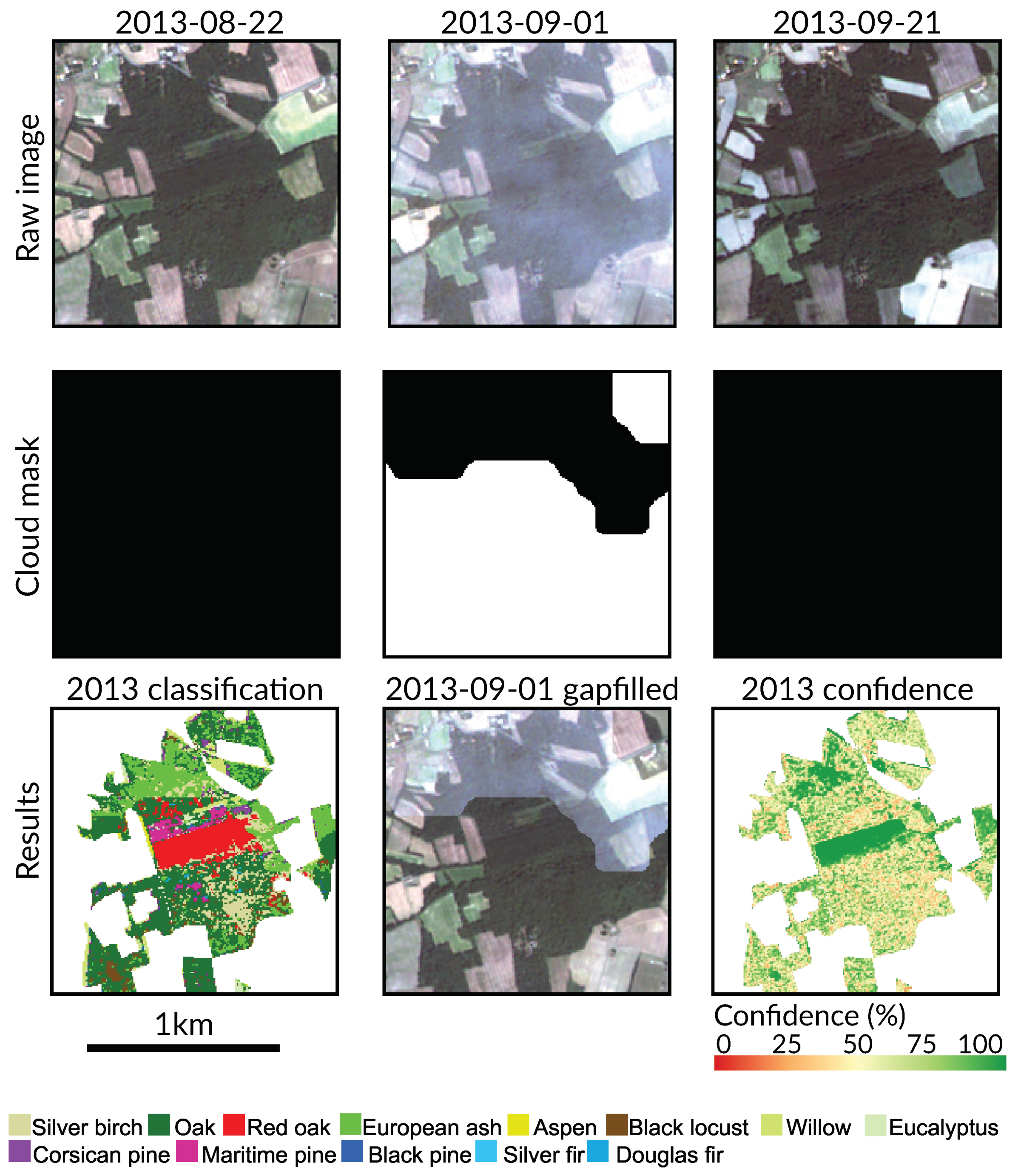
5.3. Effect of Clouds and Cloud Shadows
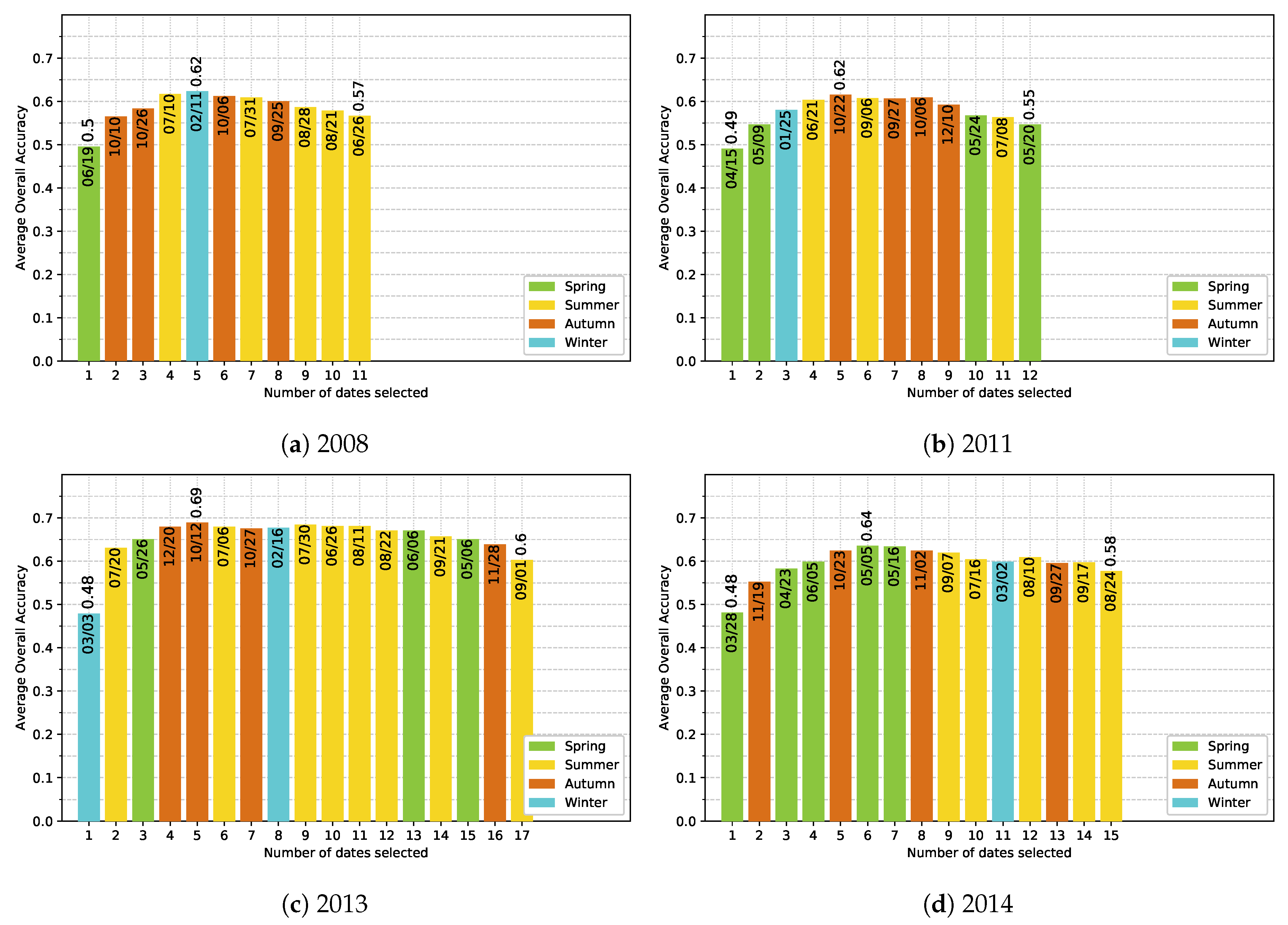
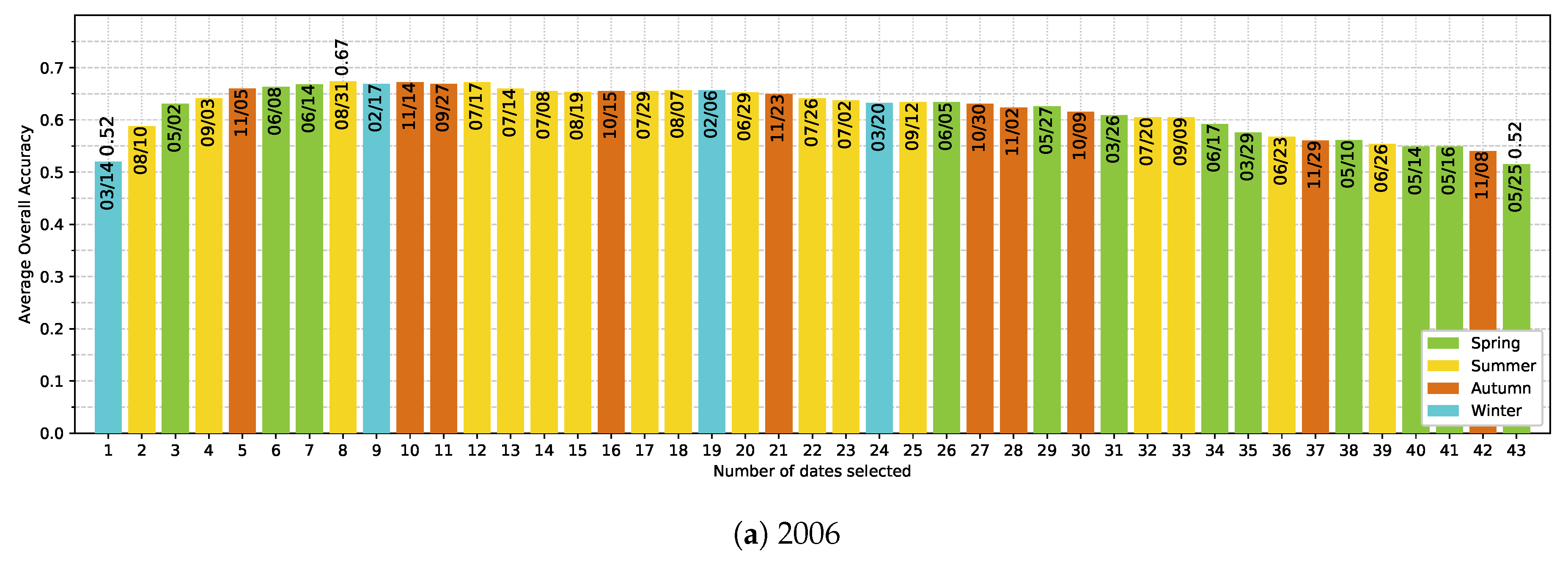
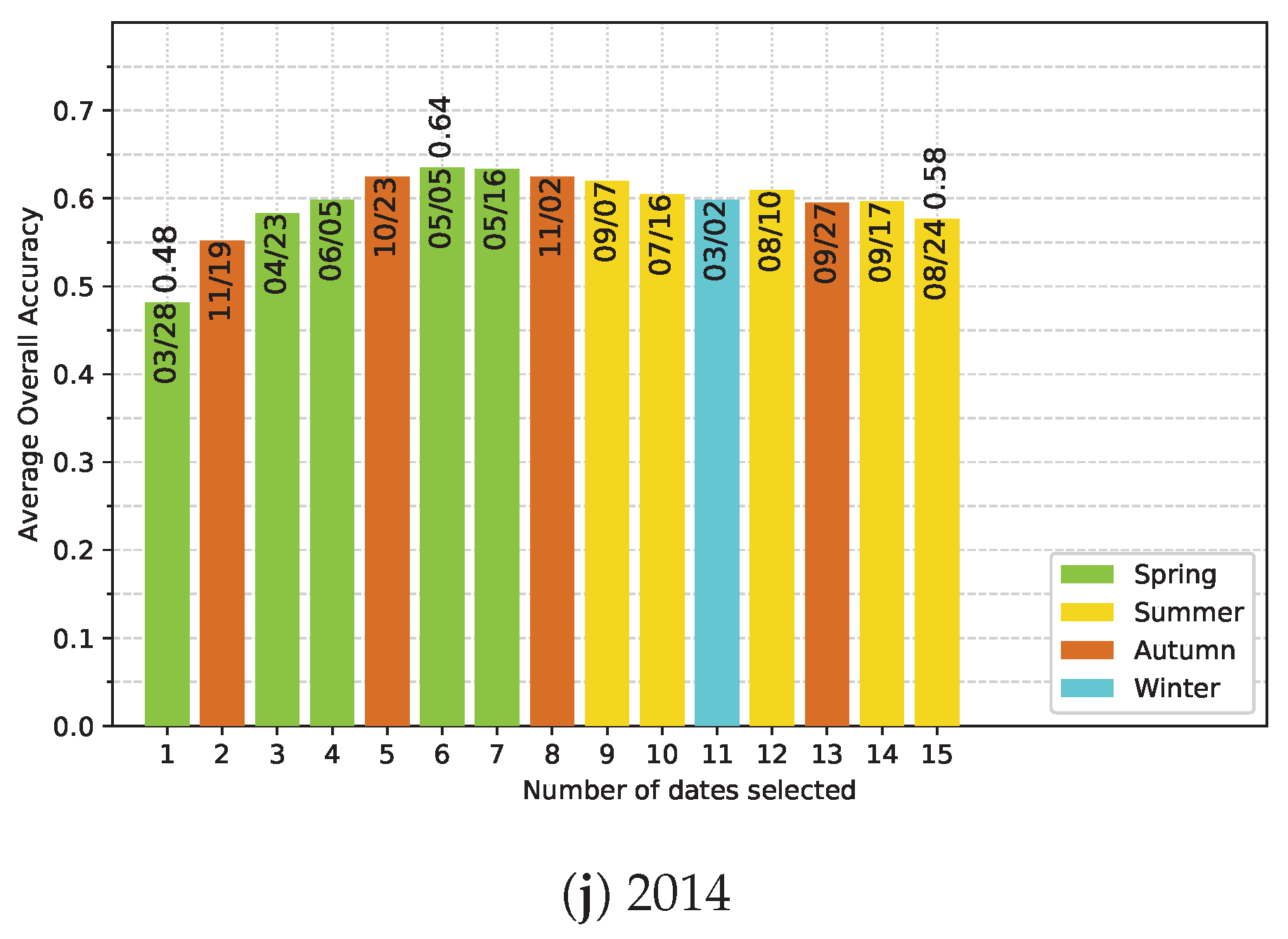
5.4. Effect of the Available Dates in the SITS
5.5. Differences between Species
6. Conclusions
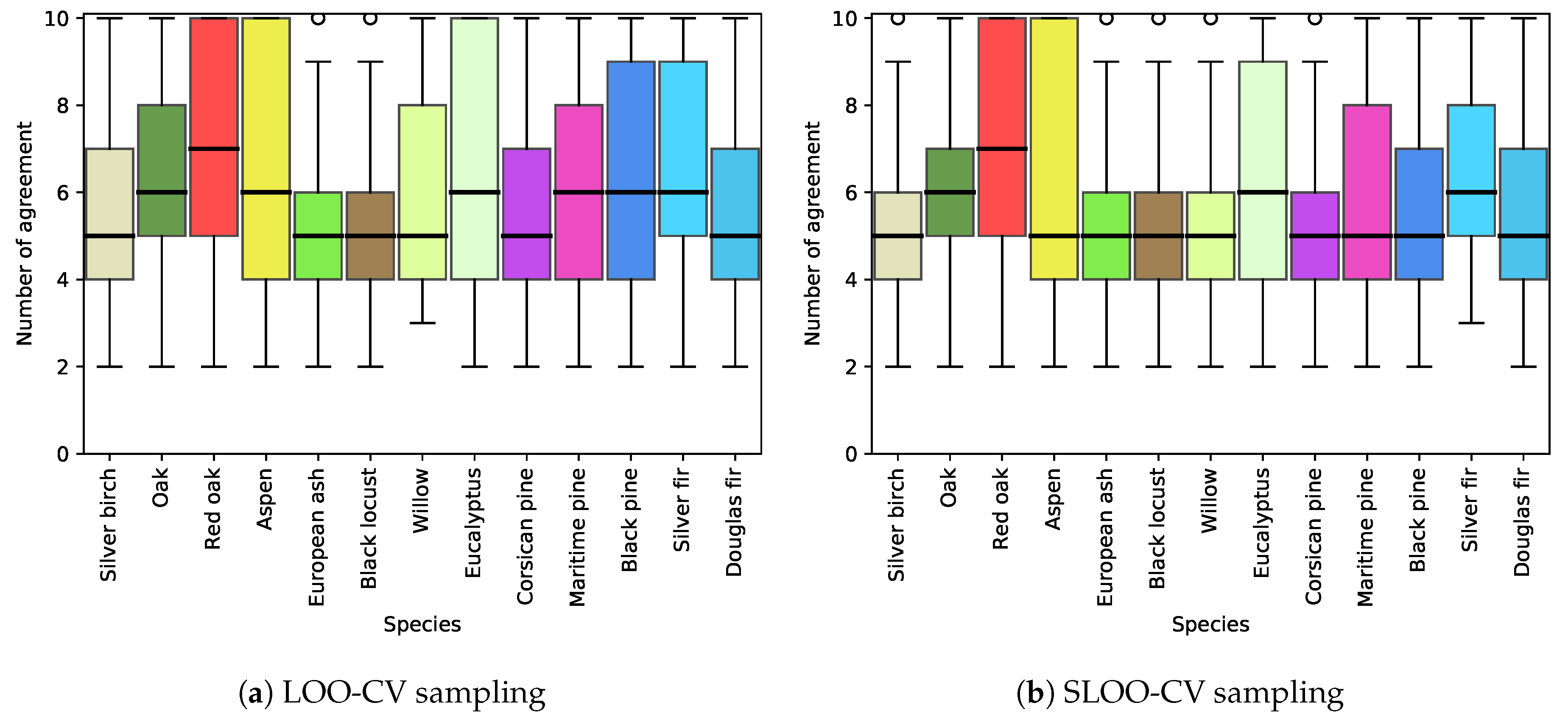
- Spatial autocorrelation within validation data drastically overestimates the classification accuracy. In our context, an average optimistic bias of 0.4 of OA is observed when spatial dependence remained (LOO-CV strategy vs SLOO-CV). In further studies, we recommend adapting the data-splitting procedure to systematically reduce or eliminate spatial autocorrelation in the validation set in order to provide more robust conclusions about the true predictive performance.
- Noise in the time series (i.e., undetected clouds and shadows) affects the SVM based classification performances. Despite accurate masks of clouds and shadows and a gap-filling approach to correct invalid pixels, residual noise impacts the learning and prediction processes. Feature selection is a good option to ignore noisy data, reduce data dimension, and to find the optimal subset of images for classification. There is a clear benefit (+0.08 of OA in average) of using fewer images containing the maximum discrimination information about the tree species classes.
- The use of multitemporal images improves the tree species discrimination compared to single-date image. However, there is no clear evidence that the positive effect is really due to phenological differences between species. The most important dates varied from one year to another with no strong preference for images acquired at the key seasons.
- The monospecific broadleaf plantations of Aspen, Red Oak and Eucalyptus are the easiest to classify. Conifers are the most difficult. The lowest accuracy was obtained for Silver birch, European ash and Black pines for which only a few forest stands were available.
Author Contributions
Funding
Acknowledgments
Conflicts of Interest
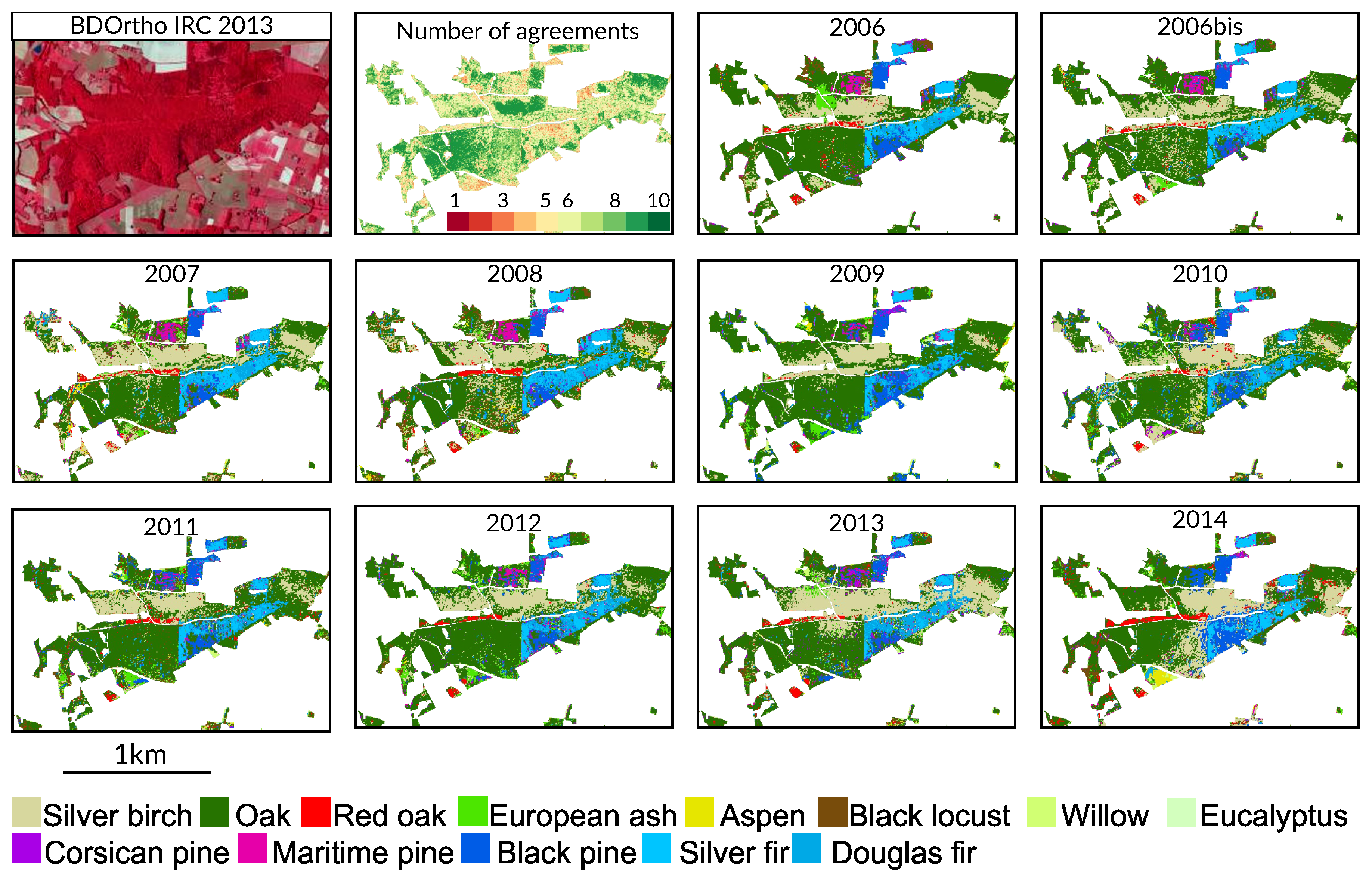
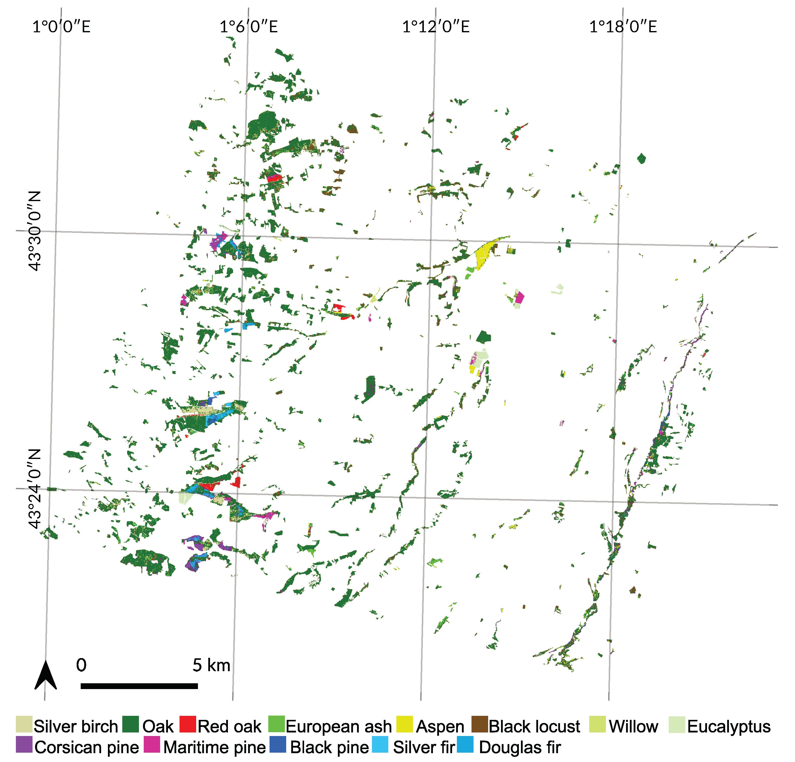
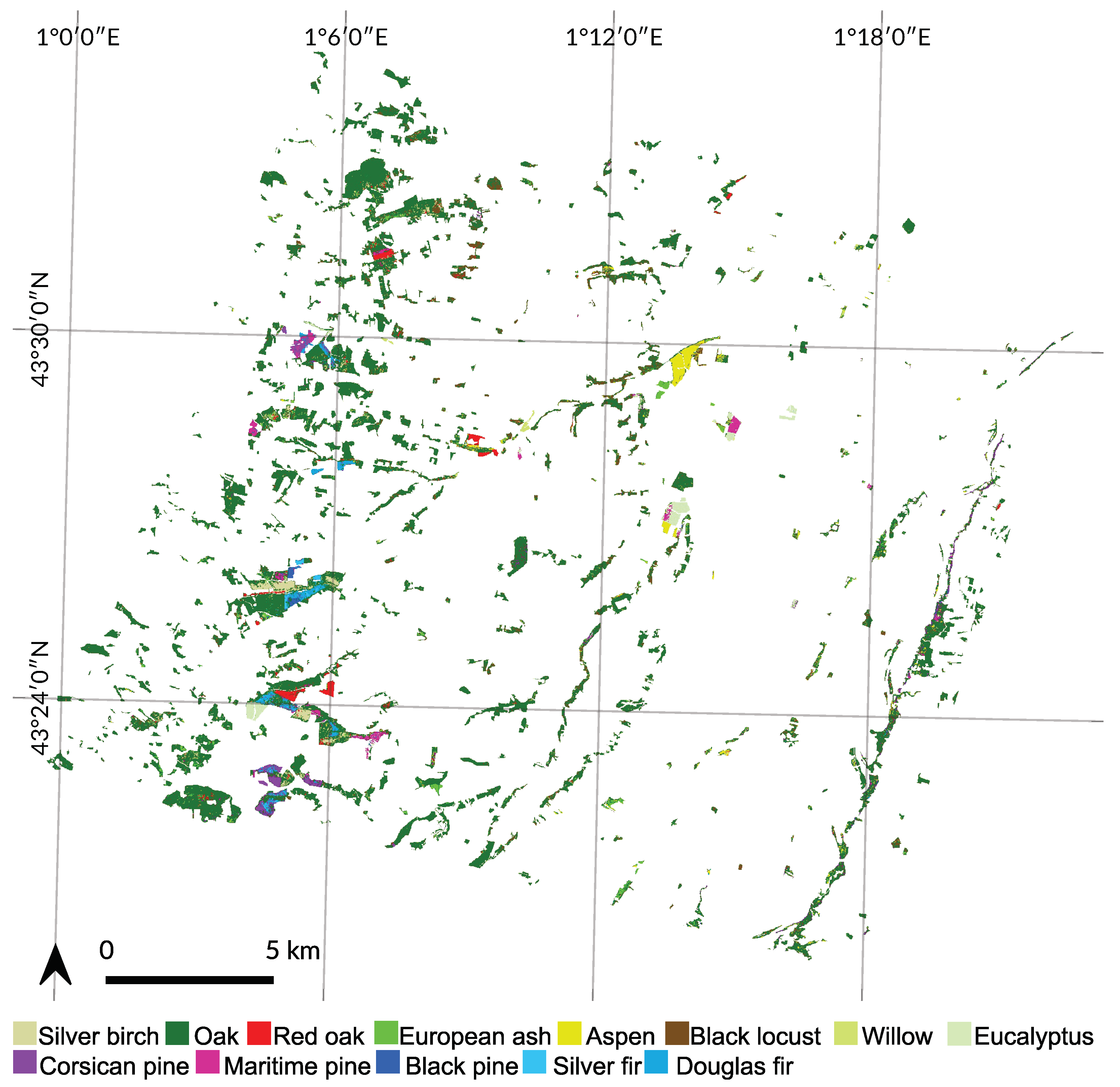
Appendix A. Tree Species Map


Appendix B. Significance Tables for Prediction between Years

| 2006 | 2006bis | 2007 | 2008 | 2009 | 2010 | 2011 | 2012 | 2013 | 2014 | |
|---|---|---|---|---|---|---|---|---|---|---|
| 2006 | nan | 244 | 242 | 255 | 302 | 354 | 313 | 194 | 193 | 309 |
| 2006bis | 244 | nan | 198 | 551 | 335 | 407 | 307 | 556 | 384 | 459 |
| 2007 | 242 | 198 | nan | 143 | 112 | 90 | 208 | 120 | 57 | 144 |
| 2008 | 255 | 551 | 143 | nan | 349 | 345 | 365 | 433 | 275 | 257 |
| 2009 | 302 | 335 | 112 | 349 | nan | 288 | 299 | 348 | 173 | 229 |
| 2010 | 354 | 407 | 90 | 345 | 288 | nan | 382 | 284 | 215 | 384 |
| 2011 | 313 | 307 | 208 | 365 | 299 | 382 | nan | 315 | 166 | 250 |
| 2012 | 194 | 556 | 120 | 433 | 348 | 284 | 315 | nan | 356 | 451 |
| 2013 | 193 | 384 | 57 | 275 | 173 | 215 | 166 | 356 | nan | 360 |
| 2014 | 309 | 459 | 144 | 257 | 229 | 384 | 250 | 451 | 360 | nan |
| 2006 | 2006bis | 2007 | 2008 | 2009 | 2010 | 2011 | 2012 | 2013 | 2014 | |
|---|---|---|---|---|---|---|---|---|---|---|
| 2006 | nan | 0 | 0 | 0 | 0 | 0 | 0 | 0 | 0 | 6 |
| 2006bis | 0 | nan | 6 | 20 | 18 | 30 | 29 | 30 | 10 | 7 |
| 2007 | 0 | 6 | nan | 4 | 10 | 0 | 6 | 5 | 0 | 6 |
| 2008 | 0 | 20 | 4 | nan | 22 | 27 | 25 | 42 | 4 | 5 |
| 2009 | 0 | 18 | 10 | 22 | nan | 30 | 11 | 32 | 16 | 11 |
| 2010 | 0 | 30 | 0 | 27 | 30 | nan | 16 | 30 | 0 | 12 |
| 2011 | 0 | 29 | 6 | 25 | 11 | 16 | nan | 16 | 6 | 7 |
| 2012 | 0 | 30 | 5 | 42 | 32 | 30 | 16 | nan | 4 | 13 |
| 2013 | 0 | 10 | 0 | 4 | 16 | 0 | 6 | 4 | nan | 7 |
| 2014 | 6 | 7 | 6 | 5 | 11 | 12 | 7 | 13 | 7 | nan |
Appendix C. Effect of Clouds and Cloud Shadows

| Species | 2006 | 2006bis | 2007 | 2008 | 2009 | 2010 | 2011 | 2012 | 2013 | 2014 |
|---|---|---|---|---|---|---|---|---|---|---|
| Silver birch | 26 | 0 | 17 | 1 | 9 | 0 | 0 | 0 | 4 | 0 |
| Oak | 24 | 0 | 20 | 11 | 6 | 5 | 1 | 0 | 2 | 0 |
| Red Oak | 21 | 0 | 11 | 0 | 1 | 6 | 3 | 0 | 0 | 0 |
| Aspen | 29 | 0 | 8 | 0 | 0 | 1 | 4 | 3 | 0 | 0 |
| European Ash | 22 | 0 | 11 | 6 | 5 | 1 | 0 | 0 | 3 | 1 |
| Black locust | 25 | 0 | 11 | 1 | 0 | 0 | 5 | 0 | 2 | 0 |
| Willow | 27 | 0 | 6 | 2 | 2 | 0 | 6 | 2 | 0 | 0 |
| Eucalyptus | 23 | 0 | 7 | 0 | 0 | 5 | 4 | 0 | 2 | 0 |
| Corsican Pine | 16 | 0 | 16 | 11 | 2 | 5 | 5 | 0 | 1 | 4 |
| Maritime Pine | 25 | 0 | 9 | 9 | 3 | 3 | 2 | 0 | 0 | 0 |
| Black Pine | 30 | 0 | 17 | 5 | 10 | 1 | 0 | 0 | 2 | 0 |
| Silver Fir | 28 | 0 | 17 | 5 | 8 | 5 | 0 | 0 | 3 | 0 |
| Douglas | 26 | 0 | 10 | 9 | 5 | 4 | 4 | 0 | 0 | 0 |
Appendix D. Training Size per Species
| Species | SLOO-CV | LOO-CV |
|---|---|---|
| Broadleaf | ||
| Silver birch | 35 | 35 |
| Oak | 97 | 97 |
| Red oak | 118 | 118 |
| Aspen | 142 | 142 |
| European ash | 50 | 50 |
| Black locust | 50 | 50 |
| Willow | 21 | 21 |
| Eucalyptus | 85 | 85 |
| Conifer | ||
| Corsican pine | 33 | 33 |
| Maritime pine | 79 | 79 |
| Black pine | 26 | 26 |
| Silver fir | 54 | 54 |
| Douglas fir | 46 | 46 |
| Total | 836 | 836 |
Appendix E. Ranking-based feature selection of Image Dates for Each Single-Year Classification


References
- Thompson, I.D.; Okabe, K.; Tylianakis, J.M.; Kumar, P.; Brockerhoff, E.G.; Schellhorn, N.A.; Parrotta, J.A.; Nasi, R. Forest Biodiversity and the Delivery of Ecosystem Goods and Services: Translating Science into Policy. BioScience 2011, 61, 972–981. [Google Scholar] [CrossRef]
- Bunker, D.E.; Declerck, F.; Bradford, J.C.; Colwell, R.K.; Perfecto, I.; Phillips, O.L.; Sankaran, M.; Naeem, S. Species loss and aboveground carbon storage in a tropical forest. Science 2005, 310, 1029–1031. [Google Scholar] [CrossRef] [PubMed]
- Thompson, I.D.; Mackey, B.; McNulty, S.; Mosseler, A. Forest resilience, biodiversity, and climate change. In A Synthesis of the Biodiversity/Resilience/Stability Relationship in Forest Ecosystems; Technical Series No. 43; Secretariat of the Convention on Biological Diversity: Montreal, QC, Canada, 2009. [Google Scholar]
- Harris, J. Soil microbial communities and restoration ecology: Facilitators or followers? Science 2009, 325, 573–574. [Google Scholar] [CrossRef] [PubMed]
- Gamfeldt, L.; Snäll, T.; Bagchi, R.; Jonsson, M.; Gustafsson, L.; Kjellander, P.; Ruiz-Jaen, M.C.; Fröberg, M.; Stendahl, J.; Philipson, C.D.; et al. Higher levels of multiple ecosystem services are found in forests with more tree species. Nat. Commun. 2013, 4, 1340. [Google Scholar] [CrossRef]
- Seidl, R.; Thom, D.; Kautz, M.; Martin-Benito, D.; Peltoniemi, M.; Vacchiano, G.; Wild, J.; Ascoli, D.; Petr, M.; Honkaniemi, J.; et al. Forest disturbances under climate change. Nat. Clim. Chang. 2017, 7, 395–402. [Google Scholar] [CrossRef] [Green Version]
- Boyd, D.S.; Danson, F. Satellite remote sensing of forest resources: Three decades of research development. Prog. Phys. Geogr. 2005, 29, 1–26. [Google Scholar] [CrossRef]
- Walsh, S.J. Coniferous tree species mapping using LANDSAT data. Remote Sens. Environ. 1980, 9, 11–26. [Google Scholar] [CrossRef]
- Fassnacht, F.E.; Latifi, H.; Stereńczak, K.; Modzelewska, A.; Lefsky, M.; Waser, L.T.; Straub, C.; Ghosh, A. Review of studies on tree species classification from remotely sensed data. Remote Sens. Environ. 2016, 186, 64–87. [Google Scholar] [CrossRef]
- Meyera, P.; Staenzb, K.; Ittena, K.I. Semi-automated procedures for tree species identification in high spatial resolution data from digitized colour infrared-aerial photography. ISPRS J. Photogramm. Remote Sens. 1996, 51, 5–16. [Google Scholar] [CrossRef]
- Trichon, V.; Julien, M.P. Tree species identification on large-scale aerial photographs in a tropical rain forest, French Guiana—Application for management and conservation. For. Ecol. Manag. 2006, 225, 51–61. [Google Scholar]
- Waser, L.; Ginzler, C.; Kuechler, M.; Baltsavias, E.; Hurni, L. Semi-automatic classification of tree species in different forest ecosystems by spectral and geometric variables derived from Airborne Digital Sensor (ADS40) and RC30 data. Remote Sens. Environ. 2011, 115, 76–85. [Google Scholar] [CrossRef]
- Immitzer, M.; Atzberger, C.; Koukal, T. Tree Species Classification with Random Forest Using Very High Spatial Resolution 8-Band WorldView-2 Satellite Data. Remote Sens. 2012, 4, 2661–2693. [Google Scholar] [CrossRef] [Green Version]
- Carleer, A.; Wolff, E. Exploitation of very high resolution satellite data for tree species identification. Photogramm. Eng. Remote Sens. 2004, 70, 135–140. [Google Scholar] [CrossRef]
- Lin, C.; Popescu, S.; Thomson, G.; Tsogt, K.; Chang, C. Classification of tree species in overstorey canopy of subtropical forest using QuickBird images. PLoS ONE 2015, 10, e0125554. [Google Scholar] [CrossRef]
- Ustin, S.; Gitelson, A.; Jacquemoud, S.; Schaepman, M.; Asner, G.; Gamon, J.; Zarco-Tejada, P. Retrieval of Foliar Information about Plant Pigment Systems from High Resolution Spectroscopy. Remote Sens. Environ. 2009, 113, S67–S77. [Google Scholar] [CrossRef]
- Ghiyamat, A.; Shafri, H. A review on hyperspectral remote sensing for homogeneous and heterogeneous forest biodiversity assessment. Int. J. Remote Sens. 2010, 31, 1837–1856. [Google Scholar] [CrossRef]
- Féret, J.B.; Asner, G.P. Tree Species Discrimination in Tropical Forests Using Airborne Imaging Spectroscopy. IEEE Trans. Geosci. Remote Sens. 2012, 51, 73–84. [Google Scholar] [CrossRef]
- Aval, J.; Fabre, S.; Zenou, E.; Sheeren, D.; Fauvel, M.; Briottet, X. Object-based fusion for urban tree species classification from hyperspectral, panchromatic and nDSM data. Int. J. Remote Sens. 2019, 40, 5339–5365. [Google Scholar] [CrossRef]
- Cano, E.; Denux, J.P.; Bisquert, M.; Hubert-Moy, L.; Chéret, V. Improved forest-cover mapping based on MODIS time series and landscape stratification. Int. J. Remote Sens. 2017, 38, 1865–1888. [Google Scholar] [CrossRef] [Green Version]
- Aragones, D.; Rodriguez-Galiano, V.; Caparros-Santiago, J.; Navarro-Cerrillo, R. Could land surface phenology be used to discriminate Mediterranean pine species? Int. J. Appl. Earth Obs. Geoinf. 2019, 78, 281–294. [Google Scholar] [CrossRef]
- Wolter, P.; Mladenoff, D.; Host, G.; Crow, T. Improved forest classification in the northern Lake States using multi-temporal Landsat imagery. Photogramm. Eng. Remote Sens. 1995, 61, 1129–1143. [Google Scholar]
- Foody, G.; Hill, R. Classification of tropical forest classes from Landsat TM data. Int. J. Remote Sens. 1996, 17, 2353–2367. [Google Scholar] [CrossRef]
- Zhu, X.; Liu, D. Accurate mapping of forest types using dense seasonal Landsat time-series. ISPRS J. Photogramm. Remote Sens. 2014, 96, 1–11. [Google Scholar] [CrossRef]
- Diao, C.; Wang, L. Incorporating plant phenological trajectory in exotic saltcedar detection with monthly time series of Landsat imagery. Remote Sens. Environ. 2016, 182, 60–71. [Google Scholar] [CrossRef]
- Pasquarella, V.J.; Holden, C.; Woodcock, C. Improved mapping of forest type using spectral-temporal Landsat features. Remote Sens. Environ. 2018, 210, 193–207. [Google Scholar] [CrossRef]
- Tigges, J.; Lakes, T.; Hostert, P. Urban vegetation classification: Benefits of multitemporal RapidEye satellite data. Remote Sens. Environ. 2013, 136, 66–75. [Google Scholar] [CrossRef]
- He, Y.; Yang, J.; Caspersen, J.; Jones, T. An Operational Workflow of Deciduous-Dominated Forest Species Classification: Crown Delineation, Gap Elimination, and Object-Based Classification. Remote Sens. 2019, 11, 2078. [Google Scholar] [CrossRef]
- Key, T.; Warner, T.; McGraw, J.; Fajvan, M. A Comparison of Multispectral and Multitemporal Information in High Spatial Resolution Imagery for Classification of Individual Tree Species in a Temperate Hardwood Forest. Remote Sens. Environ. 2001, 75, 100–112. [Google Scholar] [CrossRef]
- Hill, R.A.; Wilson, A.; George, M.; Hinsley, S. Mapping tree species in temperate deciduous woodland using time-series multi-spectral data. Appl. Veg. Sci. 2010, 13, 86–99. [Google Scholar] [CrossRef]
- Lisein, J.; Michez, A.; Claessens, H.; Lejeune, P. Discrimination of Deciduous Tree Species from Time Series of Unmanned Aerial System Imagery. PLoS ONE 2015, 10, e0141006. [Google Scholar] [CrossRef]
- Immitzer, M.; Vuolo, F.; Atzberger, C. First experience with sentinel-2 data for crop and tree species classifications in central Europe. Remote Sens. 2016, 8, 166. [Google Scholar] [CrossRef]
- Bolyn, C.; Michez, A.; Gaucher, P.; Lejeune, P.; Bonnet, S. Forest mapping and species composition using supervised per pixel classification of Sentinel-2 imagery. Biotechnol. Agron. Soc. Environ. 2018, 22, 16. [Google Scholar]
- Persson, M.; Lindberg, E.; Reese, H. Tree Species Classification with Multi-Temporal Sentinel-2 Data. Remote Sens. 2018, 10, 1794. [Google Scholar] [CrossRef]
- Liu, Y.; Gong, W.; Hu, X.; Gong, J. Forest Type Identification with Random Forest Using Sentinel-1A, Sentinel-2A, Multi-Temporal Landsat-8 and DEM Data. Remote Sens. 2018, 10, 946. [Google Scholar] [CrossRef]
- Spracklen, B.D.; Spracklen, D.V. Identifying European Old-Growth Forests using Remote Sensing: A Study in the Ukrainian Carpathians. Forests 2019, 10, 127. [Google Scholar] [CrossRef]
- Zhen, Z.; Quackenbush, L.J.; Stehman, S.V.; Zhang, L. Impact of training and validation sample selection on classification accuracy and accuracy assessment when using reference polygons in object-based classification. Int. J. Remote Sens. 2013, 34, 6914–6930. [Google Scholar] [CrossRef]
- Sheeren, D.; Fauvel, M.; Josipović, V.; Lopes, M.; Planque, C.; Willm, J.; Dejoux, J.F. Tree Species Classification in Temperate Forests Using Formosat-2 Satellite Image Time Series. Remote Sens. 2016, 8, 734. [Google Scholar] [CrossRef]
- Hammond, T.O.; Verbyla, D.L. Optimistic bias in classification accuracy assessment. Int. J. Remote Sens. 1996, 17, 1261–1266. [Google Scholar] [CrossRef]
- Chen, D.; Wei, H. The effect of spatial autocorrelation and class proportion on the accuracy measures from different sampling designs. ISPRS J. Photogramm. Remote Sens. 2009, 64, 140–150. [Google Scholar] [CrossRef]
- Meyer, H.; Reudenbach, C.; Hengl, T.; Katurji, M.; Nauss, T. Improving performance of spatio-temporal machine learning models using forward feature selection and target-oriented validation. Environ. Model. Softw. 2018, 101, 1–9. [Google Scholar] [CrossRef]
- Schratz, P.; Muenchow, J.; Iturritxa, E.; Richter, J.; Brenning, A. Hyperparameter tuning and performance assessment of statistical and machine-learning algorithms using spatial data. Ecol. Model. 2019, 406, 109–120. [Google Scholar] [CrossRef] [Green Version]
- Dedieu, G.; Karnieli, A.; Hagolle, O.; Jeanjean, H.; Cabot, F.; Ferrier, P.; Yaniv, Y. Venµs: A joint Israel-French Earth Observation scientific mission with High spatial and temporal resolution capabilities. In Second Recent Advances in Quantitative Remote Sensing; Sobrino, J.A., Ed.; Publicacions de la Universitat de València: Valencia, Spain, 2006; pp. 517–521. [Google Scholar]
- Hagolle, O.; Dedieu, G.; Mougenot, B.; Debaecker, V.; Duchemin, B.; MEYGRET, A. Correction of aerosol effects on multi-temporal images acquired with constant viewing angles: Application to Formosat-2 images. Remote Sens. Environ. 2008, 112, 1689–1701. [Google Scholar] [CrossRef] [Green Version]
- Hagolle, O.; Huc, M.; Pascual, D.; Dedieu, G. A multi-temporal method for cloud detection, applied to FORMOSAT-2, VENµS, LANDSAT and SENTINEL-2 images. Remote Sens. Environ. 2010, 114, 1747–1755. [Google Scholar] [CrossRef]
- Hagolle, O.; Huc, M.; Pascual, D.; Dedieu, G. A multi-temporal and multi-spectral method to estimate aerosol optical thickness over land, for the atmospheric correction of FormoSat-2, LandSat, VENS and sentinel-2 images. Remote Sens. 2015, 7, 2668–2691. [Google Scholar] [CrossRef]
- Grizonnet, M.; Michel, J.; Poughon, V.; Inglada, J.; Savinaud, M.; Cresson, R. Orfeo ToolBox: Open source processing of remote sensing images. Open Geospat. Data Softw. Stand. 2017, 2, 15. [Google Scholar] [CrossRef]
- Kandasamy, S.; Baret, F.; Verger, A.; Neveux, P.; Weiss, M. A comparison of methods for smoothing and gap filling time series of remote sensing observations—Application to MODIS LAI products. Biogeosciences 2013, 10, 4055–4071. [Google Scholar] [CrossRef]
- Vapnik, V.N. Adaptive and Learning Systems for Signal Processing Communications, and Control; Statistical Learning Theory; Wiley-Interscience: Hoboken, NJ, USA, 1998. [Google Scholar]
- Mountrakis, G.; Im, J.; Ogole, C. Support vector machines in remote sensing: A review. ISPRS J. Photogramm. Remote Sens. 2011, 66, 247–259. [Google Scholar] [CrossRef]
- Kavzoglu, T.; Colkesen, I. A kernel functions analysis for support vector machines for land cover classification. Int. J. Appl. Earth Obs. Geoinf. 2009, 11, 352–359. [Google Scholar] [CrossRef]
- Graves, S.; Asner, G.; Martin, R.; Anderson, C.; Colgan, M.; Kalantari, L.; Bohlman, S. Tree Species Abundance Predictions in a Tropical Agricultural Landscape with a Supervised Classification Model and Imbalanced Data. Remote Sens. 2016, 8, 161. [Google Scholar] [CrossRef]
- Pedregosa, F.; Varoquaux, G.; Gramfort, A.; Michel, V.; Thirion, B.; Grisel, O.; Blondel, M.; Prettenhofer, P.; Weiss, R.; Dubourg, V.; et al. Scikit-learn: Machine learning in Python. J. Mach. Learn. Res. 2011, 12, 2825–2830. [Google Scholar]
- Le Rest, K.; Pinaud, D.; Monestiez, P.; Chadoeuf, J.; Bretagnolle, V. Spatial leave-one-out cross-validation for variable selection in the presence of spatial autocorrelation. Glob. Ecol. Biogeogr. 2014, 23, 811–820. [Google Scholar] [CrossRef] [Green Version]
- Pohjankukka, J.; Pahikkala, T.; Nevalainen, P.; Heikkonen, J. Estimating the prediction performance of spatial models via spatial k-fold cross validation. Int. J. Geogr. Inf. Sci. 2017, 31, 2001–2019. [Google Scholar] [CrossRef]
- Moran, P.A.P. Notes on Continuous Stochastic Phenomena. Biometrika 1950, 37, 17–23. [Google Scholar] [CrossRef] [PubMed]
- Dale, M.R.; Fortin, M.J. Spatial Analysis: A Guide For Ecologists, 2nd ed.; Cambridge University Press: Cambridge, UK, 2014. [Google Scholar]
- Karasiak, N.; Sheeren, D.; Fauvel, M.; Willm, J.; Dejoux, J.F.; Monteil, C. Mapping tree species of forests in southwest France using Sentinel-2 image time series. In Proceedings of the 2017 9th International Workshop on the Analysis of Multitemporal Remote Sensing Images (MultiTemp), Brugge, Belgium, 27–29 June 2017; pp. 1–4. [Google Scholar]
- Congalton, R.G. A review of assessing the accuracy of classifications of remotely sensed data. Remote Sens. Environ. 1991, 37, 35–46. [Google Scholar] [CrossRef]
- Griffith, D.A.; Chun, Y. Spatial Autocorrelation and Uncertainty Associated with Remotely-Sensed Data. Remote Sens. 2016, 8, 535. [Google Scholar] [CrossRef]
- Mu, X.; Hu, M.; Song, W.; Ruan, G.; Ge, Y.; Wang, J.; Huang, S.; Yan, G. Evaluation of Sampling Methods for Validation of Remotely Sensed Fractional Vegetation Cover. Remote Sens. 2015, 7, 16164–16182. [Google Scholar] [CrossRef] [Green Version]
- Roberts, D.R.; Bahn, V.; Ciuti, S.; Boyce, M.S.; Elith, J.; Guillera-Arroita, G.; Hauenstein, S.; Lahoz-Monfort, J.J.; Schröder, B.; Thuiller, W.; et al. Cross-validation strategies for data with temporal, spatial, hierarchical, or phylogenetic structure. Ecography 2017, 40, 913–929. [Google Scholar] [CrossRef]
- Stehman, S. Sampling designs for accuracy assessment of land cover. Int. J. Remote Sens. 2009, 30, 5243–5272. [Google Scholar] [CrossRef]
- Lyons, M.B.; Keith, D.A.; Phinn, S.R.; Mason, T.J.; Elith, J. A comparison of resampling methods for remote sensing classification and accuracy assessment. Remote Sens. Environ. 2018, 208, 145–153. [Google Scholar] [CrossRef]
- Ramezan, C.A.; Warner, T.A.; Maxwell, A.E. Evaluation of Sampling and Cross-Validation Tuning Strategies for Regional-Scale Machine Learning Classification. Remote Sens. 2019, 11, 185. [Google Scholar] [CrossRef]
- Millard, K.; Richardson, M. On the Importance of Training Data Sample Selection in Random Forest Image Classification: A Case Study in Peatland Ecosystem Mapping. Remote Sens. 2015, 7, 8489–8515. [Google Scholar] [CrossRef] [Green Version]
- Brenning, A. Spatial cross-validation and bootstrap for the assessment of prediction rules in remote sensing: The R package sperrorest. In Proceedings of the 2012 IEEE International Geoscience and Remote Sensing Symposium, Munich, Germany, 22–27 July 2012; pp. 5372–5375. [Google Scholar]
- Cánovas-García, F.; Alonso-Sarría, F.; Gomariz-Castillo, F.; Oñate-Valdivieso, F. Modification of the random forest algorithm to avoid statistical dependence problems when classifying remote sensing imagery. Comput. Geosci. 2017, 103, 1–11. [Google Scholar] [CrossRef] [Green Version]
- Foody, G.M. Sample size determination for image classification accuracy assessment and comparison. Int. J. Remote Sens. 2009, 30, 5273–5291. [Google Scholar] [CrossRef]
- Sun, Y.; Wong, A.K.; Kamel, M.S. Classification of imbalanced data: A review. Int. J. Pattern Recognit. Artif. Intell. 2009, 23, 687–719. [Google Scholar] [CrossRef]
- Eilers, P. A perfect smoother. Anal. Chem. 2011, 75, 3299–3304. [Google Scholar] [CrossRef]
- Hermance, J.F.; Jacob, R.W.; Bradley, B.A.; Mustard, J.F. Extracting Phenological Signals from Multiyear AVHRR NDVI Time Series: Framework for Applying High-Order Annual Splines with Roughness Damping. IEEE Trans. Geosci. Remote Sens. 2007, 45, 3264–3276. [Google Scholar] [CrossRef]
- Green, A.A.; Berman, M.; Switzer, P.; Craig, M.D. A transformation for ordering multispectral data in terms of image quality with implications for noise removal. IEEE Trans. Geosci. Remote Sens. 1988, 26, 65–74. [Google Scholar] [CrossRef] [Green Version]
- Hughes, G. On the mean accuracy of statistical pattern recognizers. IEEE Trans. Inf. Theory 1968, 14, 55–63. [Google Scholar] [CrossRef]
- Melgani, F.; Bruzzone, L. Classification of hyperspectral remote sensing images with support vector machines. IEEE Trans. Geosci. Remote Sens. 2004, 42, 1778–1790. [Google Scholar] [CrossRef] [Green Version]
- Pal, M.; Foody, G.M. Feature Selection for Classification of Hyperspectral Data by SVM. IEEE Trans. Geosci. Remote Sens. 2010, 48, 2297–2307. [Google Scholar] [CrossRef] [Green Version]
- Whitney, A. A Direct Method of Nonparametric Measurement Selection. IEEE Trans. Comput. 1971, C-20, 1100–1103. [Google Scholar] [CrossRef]
- Hościło, A.; Lewandowska, A. Mapping Forest Type and Tree Species on a Regional Scale Using Multi-Temporal Sentinel-2 Data. Remote Sens. 2019, 11, 929. [Google Scholar] [CrossRef]


| Species | Sample Size | Forest Stands |
|---|---|---|
| Broadleaf | ||
| Silver birch (Betula pendula) | 85 | 3 |
| Oak (Quercus robur/pubescens/petraea) | 115 | 12 |
| Red Oak (Quercus rubra) | 147 | 7 |
| Aspen (Populus spp.) | 211 | 6 |
| European Ash (Fraxinus excelsior) | 80 | 3 |
| Black locust (Robinia pseudoacacia) | 63 | 7 |
| Willow (Salix spp.) | 50 | 3 |
| Eucalyptus (Eucalyptus spp.) | 148 | 4 |
| Conifer | ||
| Corsican Pine (Pinus nigra subsp. laricio) | 70 | 6 |
| Maritime Pine (Pinus pinaster) | 103 | 7 |
| Black Pine (Pinus nigra) | 55 | 2 |
| Silver Fir (Abies alba) | 75 | 5 |
| Douglas Fir (Pseudotsuga menziesii) | 60 | 7 |
| 2006 | 2006bis | 2007 | 2008 | 2009 | 2010 | 2011 | 2012 | 2013 | 2014 | |
|---|---|---|---|---|---|---|---|---|---|---|
| Classification accuracy (average Overall Accuracy ± standard deviation) | ||||||||||
| SLOO-CV | 0.52 ± 0.13 | 0.57 ± 0.15 | 0.48 ± 0.12 | 0.57 ± 0.10 | 0.55 ± 0.11 | 0.56 ± 0.12 | 0.55 ± 0.11 | 0.58 ± 0.14 | 0.60 ± 0.11 | 0.58 ± 0.11 |
| LOO-CV | 1.00 ± 0.02 | 0.99 ± 0.03 | 0.99 ± 0.02 | 0.98 ± 0.04 | 0.99 ± 0.03 | 0.98 ± 0.03 | 0.97 ± 0.04 | 0.98 ± 0.04 | 0.99 ± 0.02 | 1.00 ± 0.02 |
| Characteristics of each SITS | ||||||||||
| Number of images | 43 | 20 | 15 | 11 | 16 | 14 | 12 | 13 | 17 | 15 |
| Images in spring | 13 | 4 | 2 | 1 | 2 | 3 | 4 | 3 | 3 | 5 |
| Images in autumn | 10 | 6 | 4 | 4 | 3 | 4 | 4 | 2 | 4 | 4 |
| Cloud coverage | 25% | 0% | 12% | 5% | 4% | 3% | 2% | 0% | 1% | 0% |
© 2019 by the authors. Licensee MDPI, Basel, Switzerland. This article is an open access article distributed under the terms and conditions of the Creative Commons Attribution (CC BY) license (http://creativecommons.org/licenses/by/4.0/).
Share and Cite
Karasiak, N.; Dejoux, J.-F.; Fauvel, M.; Willm, J.; Monteil, C.; Sheeren, D. Statistical Stability and Spatial Instability in Mapping Forest Tree Species by Comparing 9 Years of Satellite Image Time Series. Remote Sens. 2019, 11, 2512. https://doi.org/10.3390/rs11212512
Karasiak N, Dejoux J-F, Fauvel M, Willm J, Monteil C, Sheeren D. Statistical Stability and Spatial Instability in Mapping Forest Tree Species by Comparing 9 Years of Satellite Image Time Series. Remote Sensing. 2019; 11(21):2512. https://doi.org/10.3390/rs11212512
Chicago/Turabian StyleKarasiak, Nicolas, Jean-François Dejoux, Mathieu Fauvel, Jérôme Willm, Claude Monteil, and David Sheeren. 2019. "Statistical Stability and Spatial Instability in Mapping Forest Tree Species by Comparing 9 Years of Satellite Image Time Series" Remote Sensing 11, no. 21: 2512. https://doi.org/10.3390/rs11212512