Learning Control Policies of Driverless Vehicles from UAV Video Streams in Complex Urban Environments


1
Loughborough University London, E15-2GZ, UK
2
Institute for Digital Technologies, Loughborough University London, E152GZ, UK
*
Author to whom correspondence should be addressed.
Remote Sens. 2019, 11(23), 2723; https://doi.org/10.3390/rs11232723
Submission received: 1 October 2019
/
Revised: 5 November 2019
/
Accepted: 14 November 2019
/
Published: 20 November 2019
(This article belongs to the Section Urban Remote Sensing)
Abstract
:The way we drive, and the transport of today are going through radical changes. Intelligent mobility envisions to improve the efficiency of traditional transportation through advanced digital technologies, such as robotics, artificial intelligence and Internet of Things. Central to the development of intelligent mobility technology is the emergence of connected autonomous vehicles (CAVs) where vehicles are capable of navigating environments autonomously. For this to be achieved, autonomous vehicles must be safe, trusted by passengers, and other drivers. However, it is practically impossible to train autonomous vehicles with all the possible traffic conditions that they may encounter. The work in this paper presents an alternative solution of using infrastructure to aid CAVs to learn driving policies, specifically for complex junctions, which require local experience and knowledge to handle. The proposal is to learn safe driving policies through data-driven imitation learning of human-driven vehicles at a junction utilizing data captured from surveillance devices about vehicle movements at the junction. The proposed framework is demonstrated by processing video datasets captured from uncrewed aerial vehicles (UAVs) from three intersections around Europe which contain vehicle trajectories. An imitation learning algorithm based on long short-term memory (LSTM) neural network is proposed to learn and predict safe trajectories of vehicles. The proposed framework can be used for many purposes in intelligent mobility, such as augmenting the intelligent control algorithms in driverless vehicles, benchmarking driver behavior for insurance purposes, and for providing insights to city planning.
1. Introduction
Transportation and driving of the present may become history sooner than we think as the advances of self-driving cars continue to move towards a future where owning a car and driving ourselves is obsolete [1]. Intelligent Mobility (IM) encapsulates the digital disruption of traditional transportation-related industries, such as automotive engineering, logistics, and public transportation. A key enabler of IM is the development of connected autonomous vehicles (CAVs), which are vehicles that enable navigation without assistance from humans [2]. Arguably, the uptake of connected and autonomous vehicles is ‘the greatest change to how we travel since the invention of the motor car’. Leading brands in the automotive industry have realised the potential and the inevitability of self-driving cars with many, including Ford, planning to have a “fully autonomous vehicle” on the roads by 2021 [3]. The Society of Motor Manufacturers and Traders (SMMT) 2019 Connected Report estimates that in the next 10 years, in the United Kingdom alone, current driver assistance technology and the next generation of self-driving systems will save 3900 lives and create 420,000 new jobs in automotive and related areas [4].
Another important enabling element of intelligent mobility is smart infrastructure. Smart infrastructure means that roads and intersections could be fitted with sensors and connected to a wider network of the city and vehicles within it, allowing data to be gathered, stored and shared from infrastructure to vehicles and vice versa. Smart infrastructure will enable traffic data to be collected, and analyzed for multiple purposes, such as improved city planning, automated traffic management and for providing insights to insurance purposes. For example, south in Atlanta, a 2.3-mile corridor has been set up with hundreds of Internet of Things (IoT) sensors over its 26 intersections. These sensors capture data of oncoming traffic and respond (change signals) in real-time, and in 2018 reported reducing accidents by 25%. Advancements are being made to this roadway to prepare for autonomous vehicles [5].
Autonomous vehicles rely on being provided control algorithms to handle traffic conditions that they face. They should be equipped with driving policies, which enable them to make decisions under different situations. Some of the policies are learnt by training the driverless cars under many different road conditions. However, given the nature of uncertainties associated with driving, it is extremely difficult to exhaust all possible traffic conditions and road intersections that the autonomous vehicles will have to navigate in the real world [6].
As connected autonomous vehicles (CAVs) are set to become a reality on our roads and in our cities, it is important to consider the infrastructure and how it can be used as a tool to facilitate the new age of driving [7]. Information on traffic and road conditions, including unexpected obstacles or events, can be analyzed in real-time, sent to nearby CAVs, enabling then to make a more informed decision, and therefore, improve safety and efficiency of traffic [8,9]. Smart infrastructure is becoming a reality in some states in the US, such as in Ohio, where the 33 Smart Mobility Corridor [10] plans to be the real-world playground for testing smart infrastructure and CAV systems. Smart intersections are already in use in the city of Marysville, set up by Honda [11], and by 2020 it is planned that 1800 vehicles will be equipped with connective technology allowing them to connect to each other, and the infrastructure.
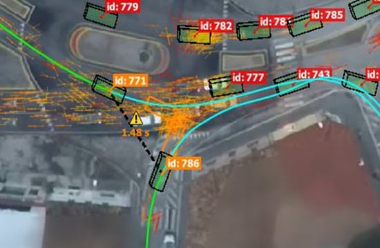
The focus of this paper is to investigate how the infrastructure can be used to learn driving policies by observing safe driving behavior of humans. We envisage a futuristic use case where the optimum policies learnt can be transferred to CAVs by the infrastructure, through high speed connections with the CAVs. This is particularly useful around complicated intersections and junctions that vehicles may have had data to be trained on. Furthermore, such a real-time policy transferring functionality can be used for centralized traffic control in smart city applications. Tesla uses the ‘fleet’ idea which means that driving experience and data is shared across all vehicles in their fleet, therefore, a single car in the fleet is not improving and updating its policies from not only it’s own driving, but also by all the cars in the fleet [12]. Using infrastructure would mean that connected autonomous vehicles would have the driving trajectories from all cars that visit that junction, the successful maneuvers would be recorded, and the optimal policy for a certain goal could be transferred to an approaching CAV. Privacy could be maintained by not recording anything about the cars on the intersection other than position, speed and type (car, motorcycle, lorry, bus, etc.). An example of a video captured from a drone, to identify the vehicle trajectories is shown in Figure 1. Also note that in Figure 1, the identities of the vehicles are anonymized.
To learn optimal driving policies, we propose to utilize data captured by the infrastructure. Data driven policy learning majorly falls into two categories: Reinforcement learning [13], and Imitation learning [14]. Reinforcement learning enables a machine to learn optimal decision-making behavior, i.e., policies, by trying to maximize rewards given by the environment it operates. Imitation learning is a data-driven policy learning algorithm, that learns optimal policies by observing expert behavior. In contrast to Reinforcement Learning, Imitation learning does not require rewards, but need to be provided examples of expert behavior. In this paper, we propose a data-driven imitation learning framework to learn driving policies from safe human-driving. In effect, we treat humans that drive safely, as experts. The contributions of this paper are, as follows:
- A new framework for infrastructure-led policy learning is proposed to augment intelligent control algorithms of connected autonomous vehicles with situational knowledge specific to a selected geo-location;
- A novel deep imitation learning framework based on long short term memory (LSTM) networks [15] is proposed as data-driven driving policy learning algorithm, by utilizing a new data set captured through uncrewed aerial vehicles (UAVs).
The rest of this paper is organized as follows: The related work are background details are presented in Section 2, and the proposed framework for infrastructure-led policy learning is presented in Section 3. The experimental details, including the dataset description, are provided in Section 4. Section 5 presents the results, and the discussion and Section 6 concludes the paper with directions for future work.
2. Background and Related Work
The following sections describe the literature related to the current contribution, followed up with background on neural networks as function approximator that will form the basis of the proposed algorithm.
2.1. Connected Intelligent Infrastructure as Enabler of Intelligent Mobility
As was discussed in the introduction of this paper, as autonomous driving advances, infrastructure will advance with it as an enabling technology. The authors of Reference [16] use discrete mathematics and V2I (vehicle to infrastructure) communication as a method to get autonomous vehicles to drive through an intersection, in this case, a symmetric four-way junction, with no collisions whilst driving continuously, and so therefore, reducing congestion and waiting time at intersections. When an autonomous vehicle approaches the intersection it will send its information, such as acceleration and velocity to the intersection manager which will in response assign it a slot, giving a minimum/maximum velocity for an approach to ensure it and other cars can all drive through the intersection, collision and interrupt free.
The study in Reference [16] assumes that all vehicles approaching the intersection have the ability to connect and send their features to the Automated Intersection Manager, however, that may not be a realistic approximation for the near future. In Reference [17], an intersection control algorithm is created for automated vehicles with the aim of safe navigation and reducing congestion at the intersection for both connected autonomous vehicles (CAVs) and human-driven vehicles. The authors hypothesize that CAVs are capable of keeping a shorter distance between themselves and the vehicle ahead (headway) more safely than human drivers can. Using this theory, along with signal phasing and timing, a headway minimization model and a signal control model is produced. The controller was tested in a simulator where the ratio of CAVs to human drivers could be changed, and it was found that the higher ratio of CAVs resulted in less congestion which suggests that the higher the population of CAVs on the road, the less traffic there would be.
Gopalswamy and Rathinam [7] argue how utilizing infrastructure greatly benefits autonomous driving. The aim of their paper is to prove that with connected infrastructure, the risk is less, safety is better, and liability is shared, therefore, there can be less hesitation with advancements, due to fear of liability issues. They propose to achieve this by implementing smart corridors where situational awareness is dealt with by the infrastructure sensors and decision making is controlled by another third party, meaning that in these corridors the driving is outsourced. As a result, if an accident were to occur, the liability is shared between multiple companies.
The papers discussed in this section so far are based on smart cities, intelligent infrastructure and connectivity of autonomous vehicles and their surroundings, in particular, the benefits of using infrastructure as enabling technology. The focus of these is on safely navigating intersections or roads with maneuvering commands sent to and from a car to infrastructure. However, V. De Silva et al. [18] propose deep imitation learning is for an infrastructure-led policy learning and communication network. The results of Reference [18] state that learning new unseen situations from other cars could improve the capability of a CAV. Furthermore, if the infrastructure was put in place to gather data from passing vehicles and share it with approaching CAVs, with relaying successful decisions for situations, it may not have come across yet. The optimal policy can be found and sent to new approaching connected vehicles. This means a CAV is not learning and updating its algorithm through its own driving and experiences alone, but through many others as well, much like Tesla does with its ‘Fleet’ [12].
2.2. Deep learning Architectures for Autonomous Driving
Neural networks are modelled on the human brain and used to process large amounts of data to make predictions, making them an ideal machine learning method for autonomous driving. Convolutional neural networks (CNNs) primarily take images as input data and can be used for classification and object recognition- a necessary component for driverless cars. In Reference [19], M. Bojarski et al. trained a convolutional neural network on data gathered from one front-facing camera. The network mapped raw pixels to steering commands and was able to drive on highways with little training data. The CNN was not explicitly fed road outlines; however, it learnt this internally and was able to drive on roads with no line markings in traffic. The authors believe that this end to end learning approach will result in better performance since ‘internal components self-optimize to maximize overall system performance’. A CNN was also created by the authors of Reference [20] which aimed to create a more human-like system to solve the problem that is a major cause of accidents for autonomous vehicles- a misunderstanding between them and human drivers. The CNN detects, recognizes and infers information from the sensors to make a decision with the data being depth information rather than RGB data as in Reference [19]. To speed up the process of training the network, the paper proposes using simulations to create training data rather than real driving data which may take many hours to collect, a strategy also used in many other papers, such as [21,22].
Advances of deep reinforcement learning with deep Q learning networks, has been proposed for driverless vehicle control [21,22,23]. A network consisting of three convolutional layers and four dense layers was created in Reference [21], and tested in a simulated urban environment made by Unity Game Engine [24]. It was used with a deep Q learning network, meaning a reward system was put in place with the aim to teach the agent to move forward, when safe, and not to hit other objects. The results from this experiment showed that the car could drive in a simulated urban environment with other cars successfully. A similar reward system was implemented in TORCS [25], an alternative simulator, by the authors of Reference [22]. The total distance travelled, and total rewards were recorded, and it was found that as training continues both the distance and rewards increase, insinuating that the more data collected, the more optimized the policy becomes. Optimizing learning is an area of great importance in autonomous vehicles, an area also discussed by Sun et al. in Reference [26] where they propose a framework that combines learning and optimization-based approaches in a 2-layer hierarchical structure. The first layer being the policy layer and the second layer is the execution layer, a controller that tracks trajectories given by the policy layer. Online imitation learning is also implemented with dataset aggregation, so the policy layer can be improved rapidly and continuously. The results are promising for situations, such as overtaking, multiple car lane situations, but intersections were not tested.
LSTMs have been used before for autonomous driving papers, such as References [27,28,29]. Multiple different variations of LSTMs are used in Reference [28] to predict the next 10 seconds of longitudinal and latitudinal trajectories of a target vehicle based on features of its nine nearest neighbors. The dataset used was a section of simulation dataset called NGSIM US 101 [30]. The features of neighbors used include velocities, distance from target vehicle, time to collision and type which are all scaled. The design of LSTM used was a 256 LSTM layer, two dense layers and time distributed layers of 256 and 128 neurons and final dense output layer containing as many cells as the number of outputs. Interestingly, to begin with the first four input features (long/lat positions and velocities) of the target vehicle were put directly into the dense layer, forgoing the first LSTM layer directly to allow the LSTM layer to focus on differences of states so that the model did not just learn the steady state of driving at constant speed. This could be since the dataset is highway driving, and the authors did not want the model to generalize. This method was found to improve quality, and the network achieved an average RMS (root mean squared error) of 70 cm for the lateral position, and less than 3 ms−1 for longitudinal velocity, 10 s in the future.
2.3. Situational Intelligence for Driverless Vehicles in Intersections/Junctions
The majority of experiments described in the papers discussed in the above section use or create data to simulate highway and straight road driving situations, where maneuvers are limited by the lack of complexity of the road structure. Intersections are more difficult to manage as an autonomous vehicle, and this section looks at research focusing on intersection management for autonomous driving.
In 2018, K. Sama et al. [31] established a method of teaching autonomous vehicles to proceed through intersections using data recorded from expert drivers and inverse reinforcement learning. It was assumed that intersections could be classified into groups, and each group requires a different driving style. Data was gathered from a car fitted with sensors and LIDAR driven by five experienced drivers through eight different intersections. These intersections were classified into groups, and the optimal driving behavior was learnt for each, for example, T junctions did not cause a sizeable amount deceleration on approach, whereas, a four-way intersection caused considerable deceleration, if not a full stop. The models were tested in a simulator and found to be successful in most cases, but scaling this method may become a problem as intersections come in a multitude of types and are handled differently in different countries or cities even.
A study by Isele et al. [23] firstly looked at how deep reinforcement learning methods compare to the Time To Collision (TTC) method in learning how to navigate unsignalized intersections using four metrics for analysis: Success percentage, percentage of collisions, the average time and average breaking time. Two deep Q networks (DQNs), such as those from References [21] and [22] were created. One was based on ‘sequential actions’ and the other on ‘time-to-go’. It was found that time-to-go outperformed the sequential action network, but both DQN methods were much better at reaching the goal than the TTC method. The second experiment described in this paper considers intersection with occlusions and how DQNs can best navigate through them. From the results of this experiment, the authors recommend that exploratory behavior, such as ‘creeping’ is needed to deal with these intersections since ‘without the ability to move to a more favorable vantage point, both TTC and Time-to-Go regularly encounter collisions’. In other words, the experimental results show that an autonomous vehicle that cannot ‘see’ its environment is less likely to proceed without fault, and therefore, needs to ‘creep’ forward at an occluded intersection, just as a human driver would do.
The research in Reference [32] tries to solve the problem of training for intersections, in general, by predicting human intentions. The authors state that LSTMs outperform state of the art methods. The paper further solidifies this statement with accuracy averaging over 85% for intersections in their experiment, which predicts human intentions as they approach an intersection. Both three- and four-way intersections were investigated where the options for a driver are to turn left, right or continue straight, and the prediction is the option with the highest probability. As was used in Reference [28], this research uses NGSIM, a simulation dataset containing positions of vehicles in intersections.
2.4. Neural Networks as Non-linear Function Approximators
Neural networks are a machine learning technique modelled on the human brain where many processing components work together to learn relationships or patterns, make predictions and deal with large volumes of data [33].
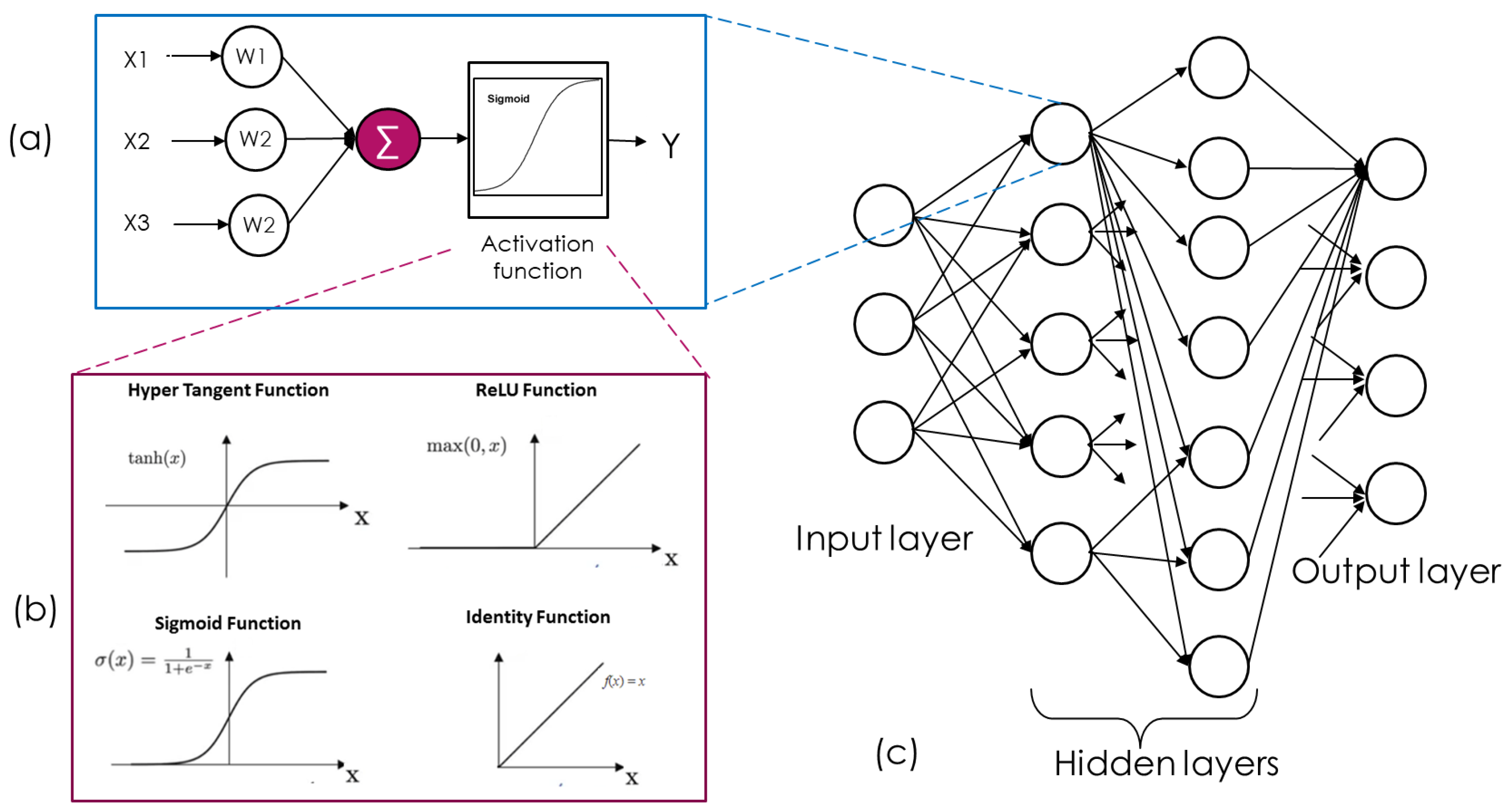
A Neural network is a collection of many simple computational units known as nodes. These nodes are arranged in a number of layers, as shown in Figure 2. There are different types of nodes, which are specialized in different types of computations. Each computation node typically has weights applied on its inputs, and an activation function which scales the weighted inputs. There are different types of activation functions, such as rectified Linear Units (ReLU), and hyperbolic tangent (tanh) and sigmoid, as shown in Figure 2b. When the neural networks with many hidden layers with many nodes are utilized, these are referred to as Deep Neural Networks. A layer of nodes that connects all its inputs to all the outputs, as shown in Figure 2c is known as a fully connected layer or a Dense layer. The performance of a NN lies in how well the weights are allocated in individual nodes.
The typical method that is used to learn the weights from example data is known as backpropagation algorithm. The backpropagation algorithm works by trying to adjust the weights of the individual nodes to minimize the difference between the target outputs and the output predicted by the network. The difference between the target output and predicted output is known as the “loss”, which can be measured using different metrics, such as Mean Squared Error (MSE). The data set is fed forward through the network multiple times, and weights adjusted through the backpropagation algorithm. Each time the dataset is fed forward through the network is referred to as an “epoch”. The backpropagation algorithm effectively is an optimization method, where the objective is to find the set of weights that minimizes the overall loss of the network. The amount by which the individual weights are updated at each epoch is determined by the error gradient at a given node. The weights are updated in the direction that minimizes the error and is known as gradient descent algorithms. There are different gradient descent optimization schemes that are utilized for this purpose, within the backpropagation algorithm. These gradient descent algorithms include, Stochastic Gradient Descent (SGD), Adaptive Momentum Estimation (ADAM), and Adaptive Learning Rate Method (ADADELTA). An overview of different methods of gradient descent algorithms can be found in Reference [34].
There are many different techniques that makes the training of deep neural networks efficient. The input data are often segmented into batches. Batch size means the number of training examples used in the estimate of the error gradient. It affects the speed of convergence and also directly affects the use of memory. For example, a batch size of 16 means 16 samples from training dataset will be used to update the gradient descent before the weights are updated. Generally, in the real-world application, when the batch size is too small, the gradient changes from time to time, which is very inaccurate and difficult for the network to converge. Then with the increase of batch size, and the gradient becomes more accurate.
Normalizing the input data of neural networks to zero-mean and constant standard deviation has is beneficial to neural network training. For improved performance in deep learning, Batch normalization extends this practice towards the intermediate (hidden) layers, but due to complexity issues normalization is performed only per mini-batch. Another important technique that is used for efficient training of neural networks is to include dropout layers. While there each node is connected to the nodes of the previous layer, as shown in Figure 2, during training, some random connections are dropped at each epoch. This is known as dropout, and is explained as a percentage of the connections that are not trained at each epoch.
2.5. Neural Network Models for Time Series Modelling
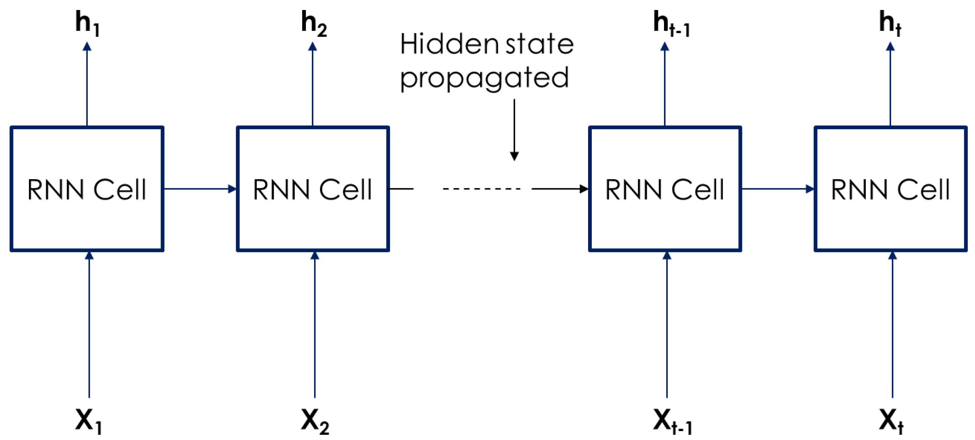
The recurrent neural networks (RNNs), a type of neural network in which the output of a previous layer is fed as part of the input to the adjacent layer [35], as shown in Figure 3.
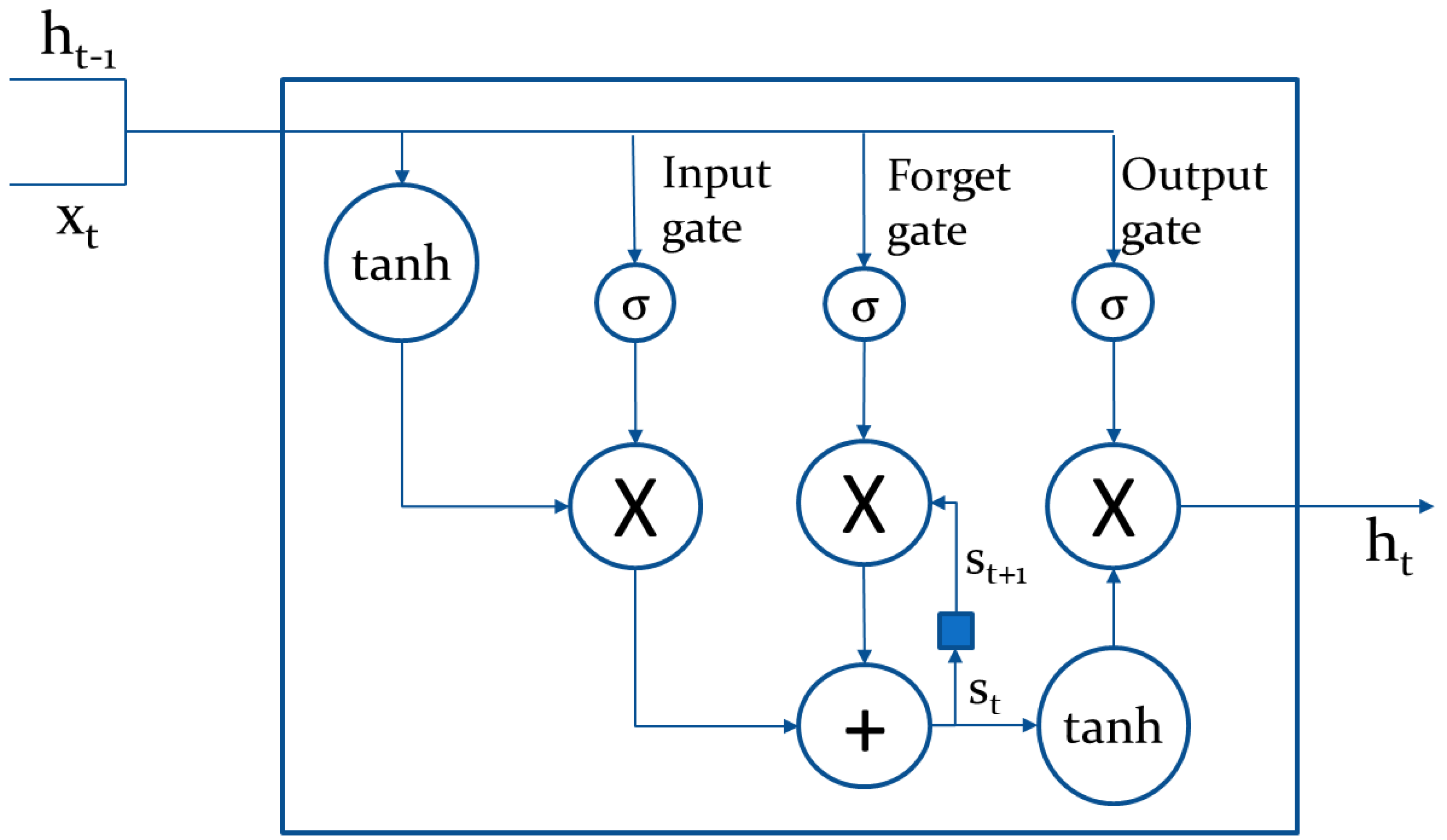
However, RNNs suffer from the vanishing gradient problem whereby the network stops learning when very small weights are multiplied repeatedly, and therefore, tend to 0. The result of this is that the weights of primary layers do not vary greatly, and the network lacks the ability to learn long-term dependencies [36]. Long short-term memory networks (LSTMs) are a branch of RNNs with nodes of a special structure, which effectively overcomes the vanishing gradient problem. LSTMs were introduced in a 1997 paper written by Hochreiter and Schmidhuber [15], and solve the vanishing gradient problem since they can learn long term dependencies, due to the addition of three gates; input, forget and output.
Figure 4 shows an individual LSTM cell [37]. Going from left to right, we see that the inputs are the current input data xt, and the output ht−1 from the previous cell, which is scaled between −1 and 1 using a tanh activation function. The input gate uses sigmoid activation functions (scales between 0 and 1) essentially to filter what information continues, expressed as:
W represents weights and b, the bias. This output it, from the input gate is then multiplied together with the output of the tanh activation function. Moving along the top line to the forget gate, this gate uses sigmoid activation function to choose what information to pass through and what to ‘forget’. This can be expressed as:
The output of the forget gate is then multiplied by the internal state of the previous cell St−1 and then added to the result of the first multiplication to produce the current cell state, St:
This addition is what allows LSTMs to avoid vanishing gradients since weights are not multiplied together. To produce output ht, the inputs go through another sigmoid activation function just as in the input and forget gates, called the output gate. This is then multiplied by the result of tanh activation function acting on the internal cell state St.
LSTMs and RNNs, in general, are used for time-based series or sequences, such as stock trends and language and more recently, autonomous driving which is the focus of the research.
2.6. Summary
This literature review looked at various research papers written on the broad topic of autonomous driving, separating into smaller categories for the purpose of this research. What was clear across all papers was that neural networks and LSTMs, in particular, are a good choice for experiments, with Reference [32] reporting that LSTM outperforms state of the art methods. Results in References [22,26] agreed that more data improves the driving algorithm, as was seen as an underlying results in all papers. The final section saw that smart infrastructure could be a useful enabling technology for CAVs. Authors of References [7,16,17] agree that infrastructure should be used in the new age of autonomous driving, whether for better intersection management to ease congestion or to share liability. Specifically, the research in Reference [18] suggests that infrastructure can be used as a tool to optimize policy learning within CAVs, and this theory is what this dissertation aims to take further.
3. Proposed Framework for Infrastructure-led Driving Policy Learning
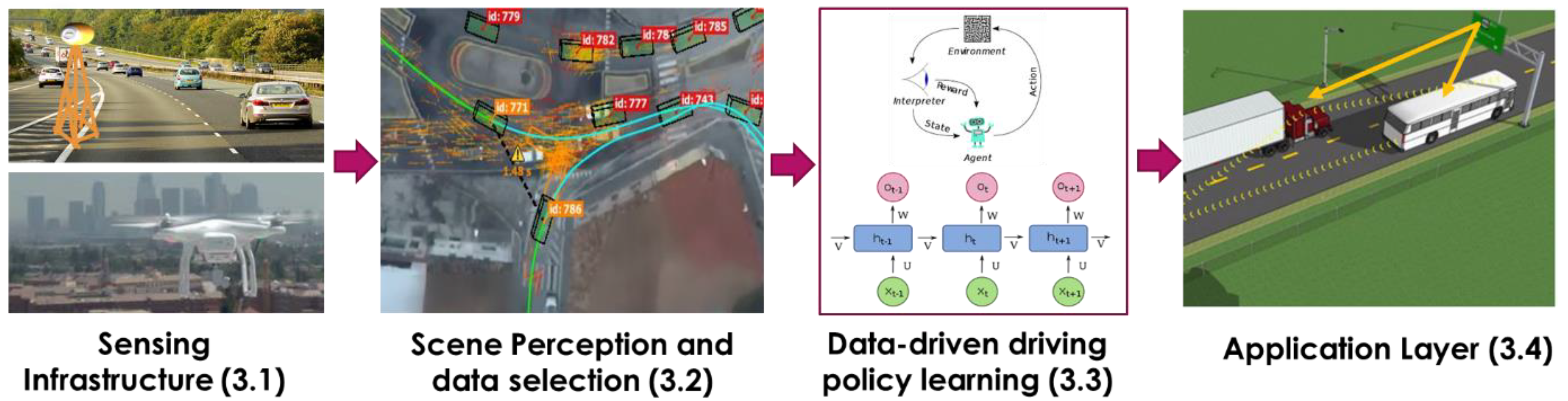
This section describes the proposed framework for learning driving policies from data gathered through the infrastructure. The proposed framework is summarized in Figure 5, where the four major elements are data capturing, pre-processing, driving policy learning and application layer. Each of these elements is explained in the following sub-sections.
3.1. Data Capturing and Processing
The first element of the proposed architecture is to capture appropriate data. The most practical source of data would be video data streams captured through cameras positioned on roadside infrastructure. One emerging source of data for such purposes may originate from UAVs equipped with cameras. The most obvious advantage of using UAVs for the purpose of traffic video capturing is that it can be deployed on request. For example, when there is an accident or a roadblock obstructing the free flow of traffic, real time data can be gathered. Another data source appropriate for the task is Geographic Positioning System (GPS) tracking data. However, collecting such GPS tracking data would require that each vehicle to transmit its position, which may not be practical. Furthermore, video data enables to capture not only the vehicle movements, but also the movements of pedestrians and cyclists. In the current demonstration, we shall utilize a video dataset captured from UAVs. More information about the dataset can be found in the next section.
3.2. Scene Perception and Extraction of Expert Data Trajectories
The next block of the proposed framework is to extract scene information from the video stream as suitable for data-driven policy learning. The scene information to be extracted are the vehicle type, pedestrian identification, distance to nearby vehicles, speed of the vehicles, and trajectories of vehicles. Once such details are extracted from the video streams, the next step is to identify examples that reflect safe driving. Most important criteria to be applied to identify safe driving examples is when vehicles are not involved in a crash/accident. Further criteria may be applied to extract a subset of vehicle trajectories that reflect safe driving, such as, when a vehicle is traveling too fast, or it is traveling too slow, or the vehicle shows unsafe behavior, such as excessive or sudden acceleration/deceleration. As such, this step involves identifying vehicle trajectories that may act as examples of safe driving behavior, and thus, forms a collection of expert data trajectories. The proposed algorithm for expert data trajectory extraction is given in Algorithm 1.
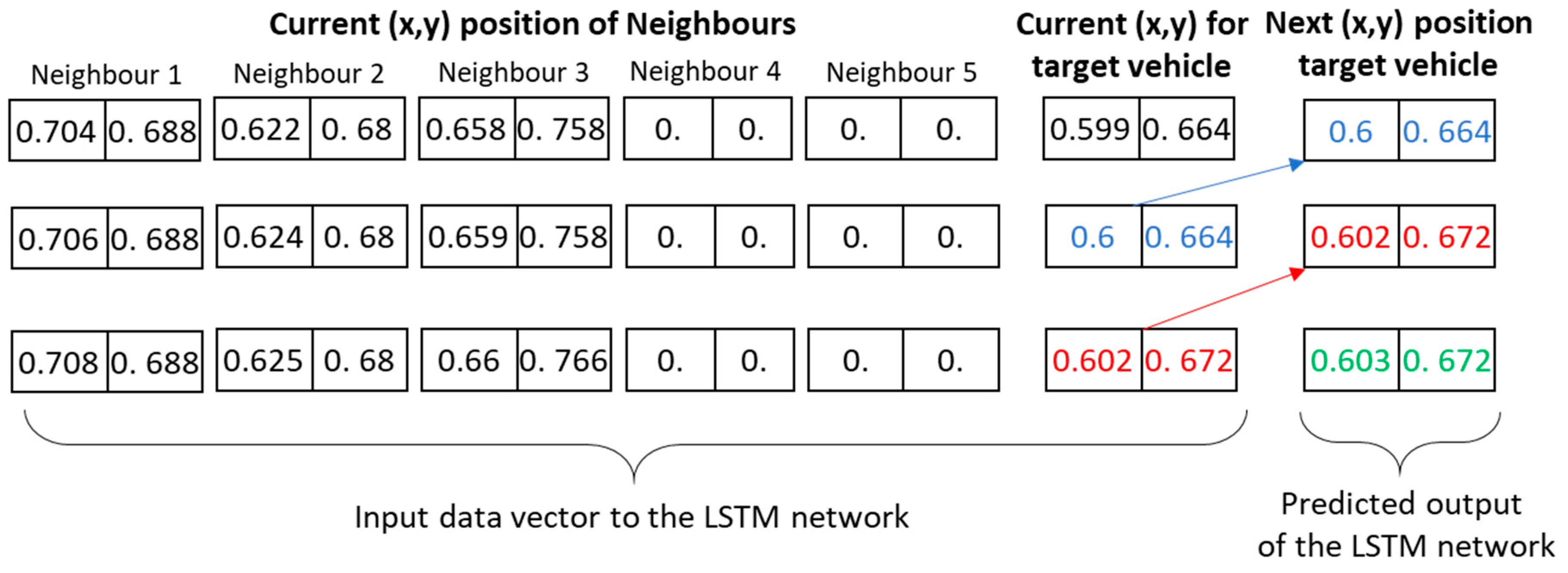
In the demonstration of this paper, the functionality of DataFromSky viewing software [37] is used for scene understanding, including to obtain the time to collision (TTC) between two as a measure of safe driving. In other words, video understanding algorithm is utilized to convert the videos from the UAV to extract the individual vehicle trajectories. The output of this step is, thus, a data field corresponding to the vehicle/pedestrian positions at each time step of the video sequence. To create a data frame for each target vehicle, the trajectory of the given vehicle is augmented with additional information about the neighboring vehicles at each time step. The result of this step is illustrated in Figure 6. This dataframe is utilized for the policy learning task in Section 3.3.
| Algorithm 1. Extraction of Expert Data Trajectories |
Input: Object Tracking data: Positions of vehicles at each timestep with a tracking id
|
3.3. Data-Driven Policy Learning
The next element of the proposed framework is to utilize the extracted example vehicle trajectories to learn driving policies. Generally, there are two classes of data-driven policy learning algorithms that can be used for this purpose. Firstly, the data-driven policy learning problem can be framed as a reinforcement learning algorithm. For this purpose, it is necessary to define an appropriate reward function that relates to the utility of being in an environmental state. In real-world driving environments, it is difficult to define a reward function, as motives of individual drivers can be very different, such as some may prefer to travel fast, and some may prefer to travel slow. Another option is to employ a global measure of utility, such as overall fuel efficiency, or congestion, but such reward functions often are unrealistic, unless in a futuristic scenario where the entire vehicle population in a local environment is controlled by a central authority.
An alternative approach to driving policy learning is to frame the problem as an imitation learning problem, where the policies are learnt by observing experts. The expert data trajectories extracted in Section 3.2, will act as examples for learning the policy. In the proposed implementation, the driving policy learning is framed as an imitation learning problem, where a given vehicle is considered as an agent in the environment. The agent is modelled as a time series prediction, where the objective is to predict the future trajectory of the agent, given the past trajectory and the proximity of neighboring vehicles. An LSTM network is trained and used for time series prediction in the current demonstration. More information about the data structures used and the LSTM network architecture is presented in the next section.
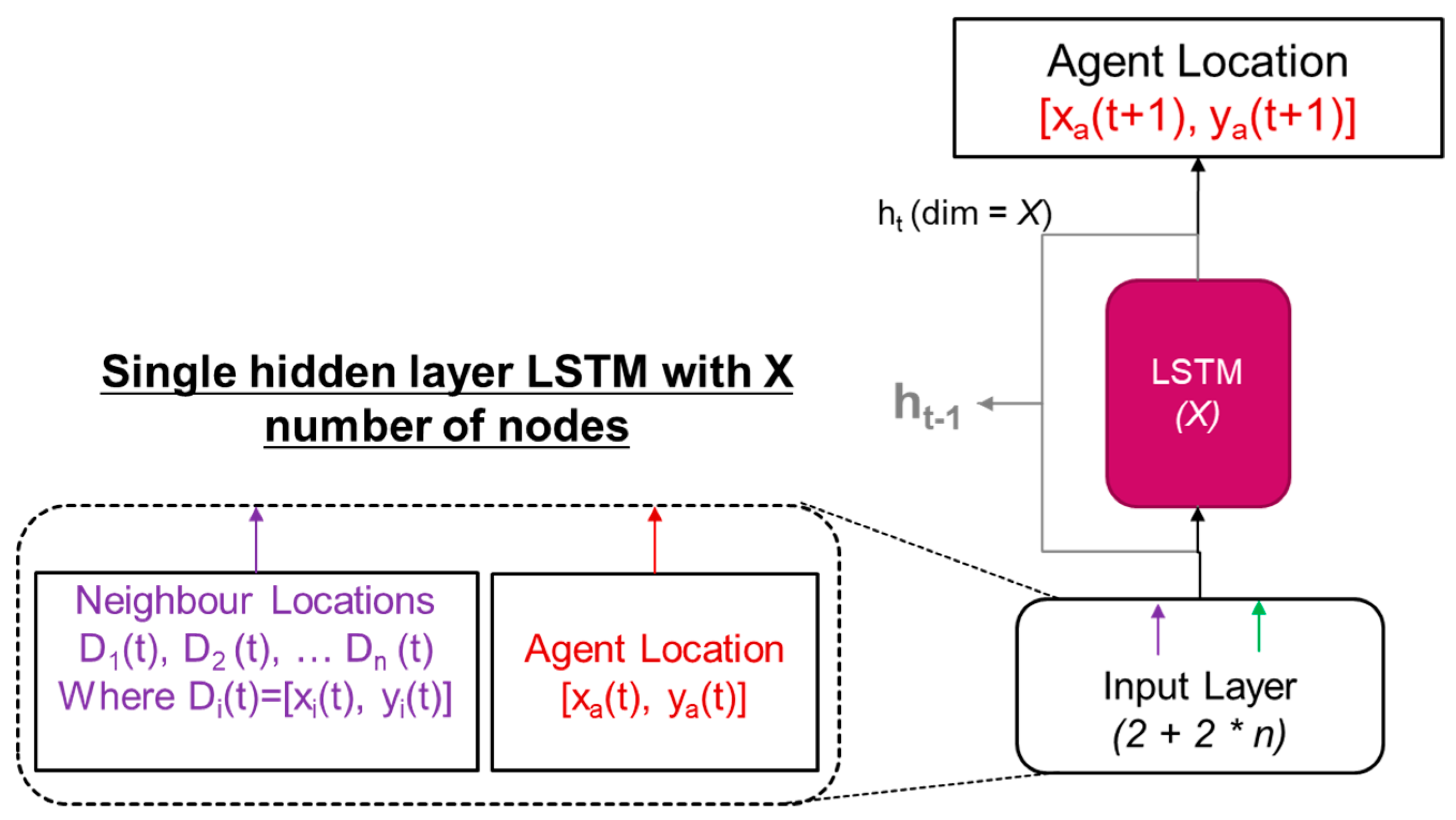
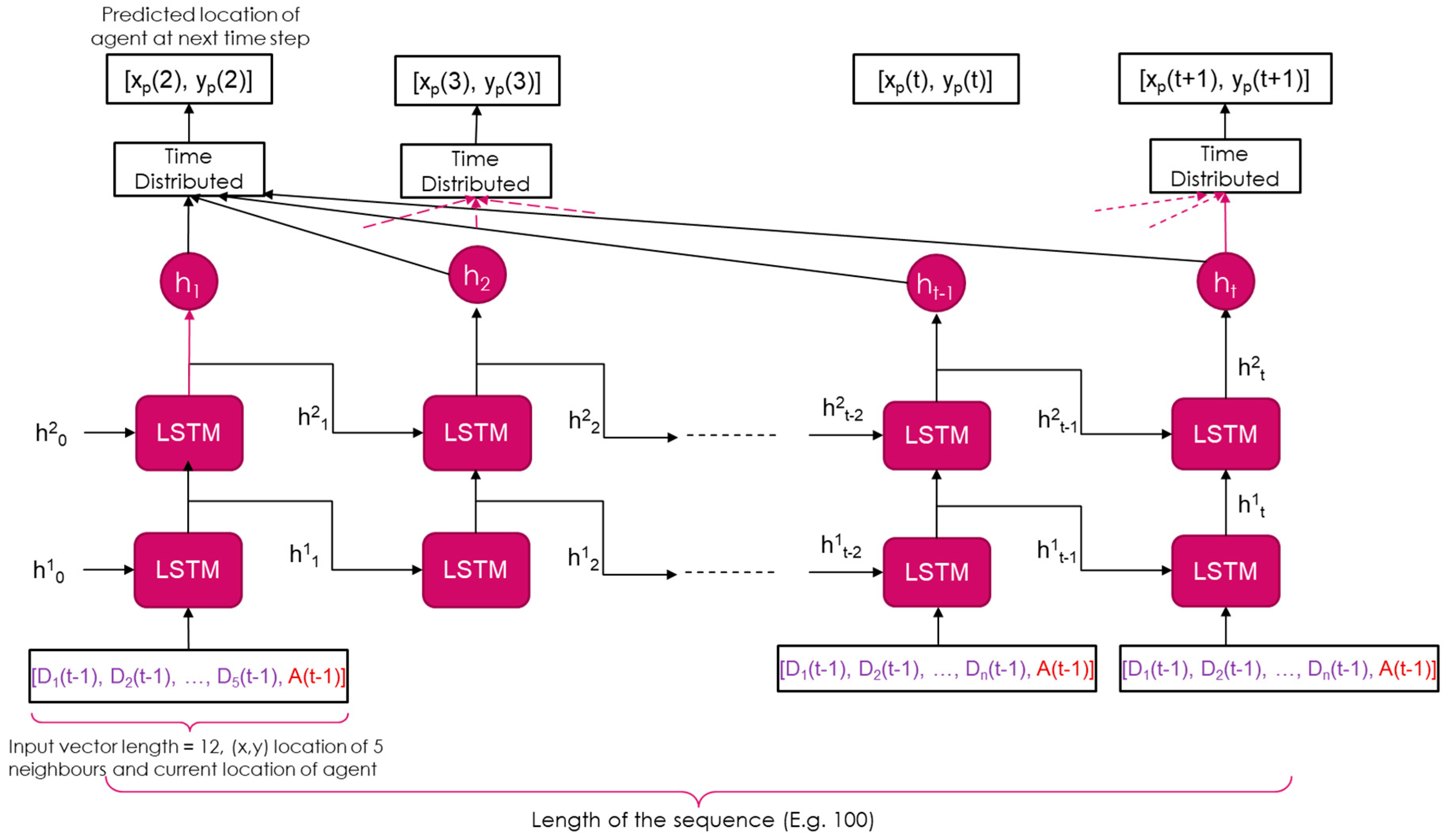
The function approximator task of the LSTM network is to predict the next location of the target vehicle, given the current locations of neighboring vehicles and the target vehicle. The data structure used for the current implementation of LSTM network is given in Figure 6. Accordingly, the input data frame contains the spatial location of five nearest neighbors and the current position of the target vehicle. The expected output is the next spatial location of the target vehicle. The structure of the LSTM network is shown in Figure 8.
3.4. Application Layer
The application layer can be configured for any appropriate purpose. The application layer will utilize the learnt driving policies for a variety of services. For example, the learnt driving policies can be used to gain insights on the safety of certain road intersections, thus, informing city planners. Another useful, futuristic application is to augment the intelligence of driverless cars, by transferring the most up-to-date driving policy at certain intersection/junction, when the car approaches the junction. This is especially suitable when the traffic conditions at a certain junction are very dynamic and unusual. The demonstrations of this paper are focused on the Section 3.2 to Section 3.3 in the above descriptions.
4. Experimental Details
This section describes experimental details pertaining to the proposed methodology.
4.1. The Dataset
The dataset was commissioned to be captured by DataFromSky [38], and consists of five video sequence sets, taken from drones over three unique intersections around Europe, from Italy and Denmark. The data is then anonymized, and the vehicle tracking details are provided in a proprietary tglx format, which can be opened using proprietary software in which each frame is able to be viewed. The software allows users to select trajectories, define gates and export information into a csv file. Gates are used to defining entrance and exit and direction of a vehicle on an intersection. The trajectories can be extracted from the software in a CSV file with the following features: Unique vehicle ID, vehicle type (Bicycle, Motorcycle, Car, Medium vehicle, Heavy vehicle, Bus), the entry gate and the exit gate, spatial location given by (X and Y position), velocity, lateral acceleration, longitudinal acceleration, timestep at 40ms intervals.
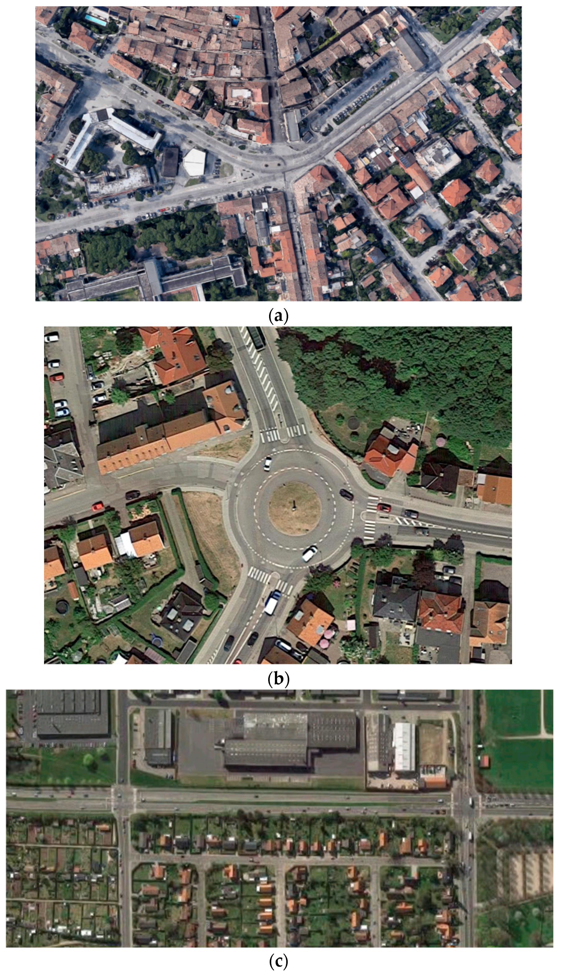
The three videos were taken of the Italy intersection as shown in Figure 9a at GPS coordinates 43.839917, 13.019667, were acquired over different conditions, including day, night, light traffic and heavy traffic. The videos have an average length of 2 h 20 m and captured tracks for a maximum of 9362 vehicles for one video. Furthermore, videos were captured from two different geographic positions, as shown in Figure 9b,c (at GPS Locations 55.406289, 11.341097, and at 55.858421, 9.824669, respectively). Denmark Intersection videos were 2 h 5 m and 1 h 41 m and tracked 3400 and 5097 vehicles, respectively.
4.2. Data Pre-processing
The pre-processing of the first dataset is discussed in more detail than the others since they followed the same method, but any changes and modifications are stated.
The dataset chosen to use first was a daylight video from the Italy intersection consisting of 3792 vehicles tracks over a period of 2 h 20 m with varying levels of traffic. Five entry and exit gates were defined using the software, and these gates are used to define a specific maneuver. For example, one maneuver chosen for the demonstration is entering at gate A and exiting gate at E on Figure 10.
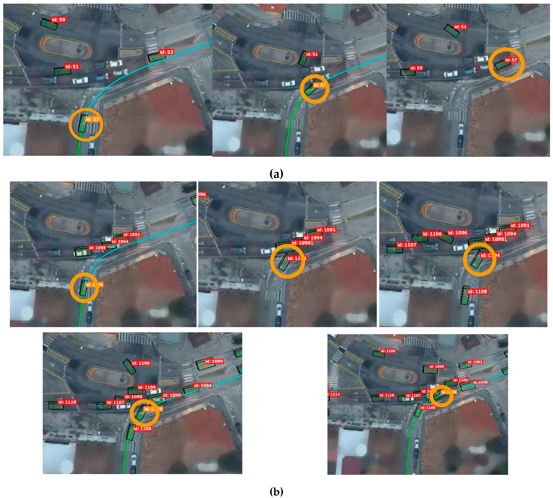
Figure 11a,b show examples of a target vehicle performing the maneuver successfully in different traffic conditions. Car with ID 57 could join the main road with little braking and no stopping time since there were no oncoming cars. Car with ID 1104 approached the entrance and stopped as cars were blocking the entrance. It then had to wait until the car blocking its front moved, by which time several other vehicles had entered its vicinity, and it now needed to slot in between two cars. Please note that these images in Figure 9; Figure 10 are obtained by superimposing tracked vehicles as rectangles on a static image of the location. As such, please note that cars that can be seen in the background are coming from this static image and are not in motion at the given time frames. The vehicles shown as black boxes with ID tags are the ones in motion and are considered in this modelling task.
4.3. The Neural Network Model Building
Neural network architecture details and terminology.
The terminology used in this section and in results Section 5, is consistent with the background information provided in Section 2.4 and Section 2.5. The neural network architecture used in these experiments is LSTM networks. We use the python packages Tensorflow [40], and Keras [41] to create and train these neural networks.
The general structure of a neural network, as given in Table 1, Table 2 and Table 3, is shown in Figure 12. It should be noted that Figure 12 is the same as Figure 8, but Figure 12 is known as the rolled out version of Figure 8. Figure 12 shows what happens at each time step, where the LSTM network computes a hidden state (denoted by hXT in Figure 12, where X denotes the layer number, and T denotes the time step) by using the current input and the hidden state from the previous time step. It is important to note that there is only one LSTM network that produces the hidden states. Furthermore, there can be more than one layer of LSTM nodes, as is shown in Figure 12. The example in Figure 12 is synonymous with Neural Network of type in Table 2. Moreover, note that within one block of LSTM there are a different number of nodes or LSTM cells, as shown in Figure 4. For example, in the neural network defined in Table 1, there are 10 LSTM cells. This layer of LSTM cells (nodes) is followed by dropout and batch normalization functions.
The return_sequences function in Table 1 to Table 3, means whether the hidden state of each time step is returned as an output, or not. For example, in all our networks return_sequences was true meaning that the hidden state is returned. Alternatively, the hidden state may not be returned at each time step, but only at the end of the sequence, i.e., only ht in Figure 12 is returned to the above layers. Time distributed layer works as a linear combination of the hidden states of all the timesteps. As such, the final output of the network is a linear combination of all the hidden states from the LSTM nodes at each time step.
The training of all the neural network architectures is performed through the Adaptive Gradient Descent Optimization algorithm, often denoted as ADAM [42]. The following parameters are necessary to be set for appropriate operation:
Learning rate: The proportion by which the weights are updated. Larger values result in faster updating of weights. When the learning rate is set too low, the convergence process will become too slow. When the learning rate is set too high, the gradient may oscillate back and forth around the minimum value, and may even fail to converge.
Decay rate: Refers to the proportion by which the learning rate is changed over time.
Beta 1 and Beta 2, refer to the exponential decay rate for the first and second moment estimates, respectively. As Reference [42] suggests, 0.9 and 0.999 as appropriate values for beta 1 and beta 2, respectively.
Epsilon is a very small value that is used to prevent division by zero.
Training and validating neural network architectures
Python 3.7 [43] was used to pre-process the data using libraries, such as NumPy, pandas and scikitlearn in Jupyter Notebook [44].
Throughout the training process, the dataset was run through a variation of the model, and then the model was amended to achieve better results. Better results, in this case, refer to the model achieving high accuracy, good bias-variance trade-off, not overfitting and having low losses. Overfitting is when the accuracy for the training dataset is much higher than that of the validation dataset meaning the model has learnt particulars for that training set and will not perform well on unseen test data. The following changes were experimented with and made at various times to try and increase accuracy and avoid overfitting:
- Changing the architecture by adding/removing/shuffling layers;
- Changing learning rate, decay rate, and different loss functions;
- Increasing or decreasing number of epochs and/or batch size;
- Changing data pre-processing, timesteps, sequence size, decimal places.
Multiple neural network architectures were tried out with a number of changes made to training hyper parameters, the best-found parameters and architectures will be presented in the results section.
The dataset is made up of the example trajectories. The dataset is segmented into a training set and validation set. The training set is used to learn the weights of the neural network at a given run (epoch) by trying to minimize the loss. Once a set of weights is determined, the effectiveness of these weights is measured by checking the trained network performance on the validation set. Note that the validation set is not used for training the weights, and hence, act as a verification method. The ratios used were 10% for testing, 30% for validation and 60% for training. Data was shuffled every epoch using the package random and shuffle function. The indexes for inputs and outputs were shuffled in the same way and then used to shuffle data to ensure the inputs still owned the same index as its corresponding output.
5. Results and Discussion
In the following sections, we describe the results obtained from policy learning algorithms and discuss the implications of them.
5.1. Driving Policy Learning
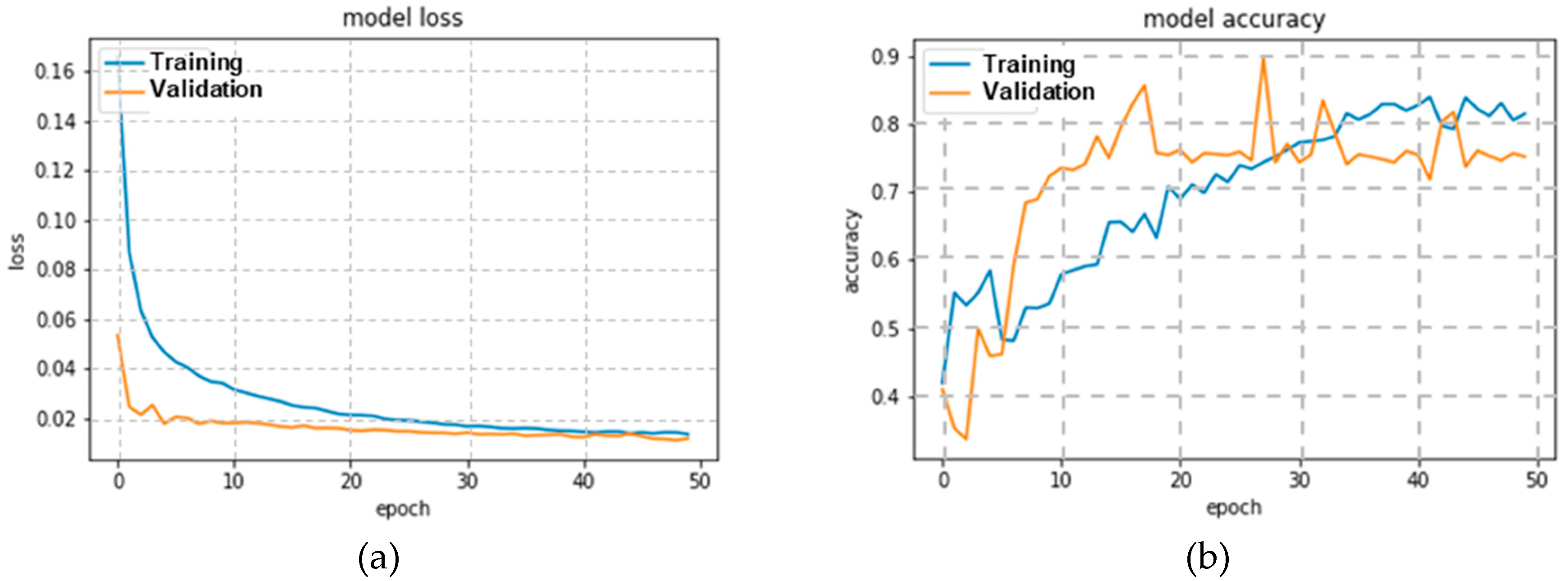
For each of the intersections considered, different LSTM network architectures were tried out. For the first intersection, i.e., Italy junction, multiple different network architectures were considered, and the best model was selected based on the cross-validation performance. The best network architecture that was obtained for Italy junction is given in Table 1, and the corresponding cross-validation curves are provided in Figure 13.
5.2. Comparison of the Models
Overall the architectures are very similar, with a small difference in activation functions of LSTM cells and addition of batch normalisation layers or even a dense layer for the Italy model. The architecture used for the Italy dataset was the largest and most complex and yet gave the least accurate results. All datasets were able to be pre-processed successfully and run through a neural network. The final accuracies and losses are summarised in the Table 4 below.
5.3. Discussion of Results
The purpose of the driving policy learning experiments was to illustrate that a position predictor can be learnt effectively from extracted data trajectories. The cross-validation results produced illustrates that models can be learnt with a good bias-variance tradeoff, and good accuracy. This means that we can utilize LSTM networks as an effective function approximator to predict vehicle movements.
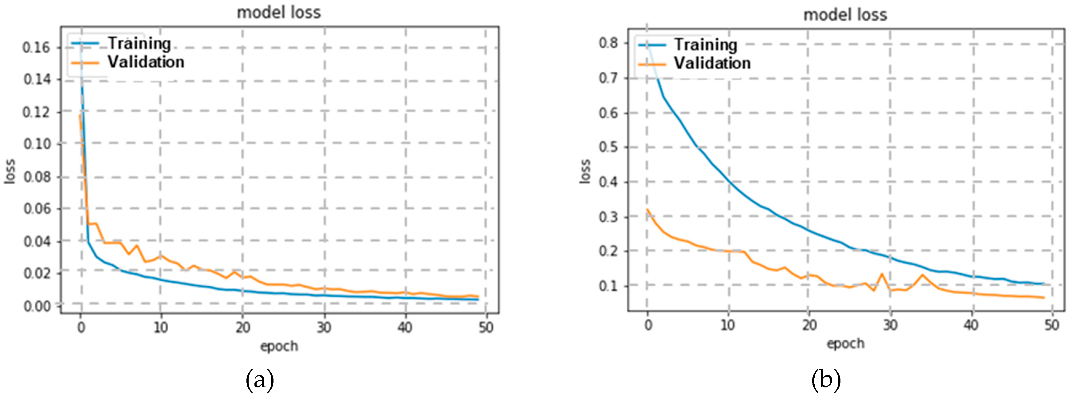
The training and validation accuracy of Denmark-A dataset show that high accuracy can be achieved, at low loss. This indicates that the variance in the dataset is limited, which is mainly due to low levels of traffic during the time of capture. Whereas, in the Italy dataset, the accuracy levels are low, and this is mainly because the Italy data set has high traffic at the time of capturing.
Also, noteworthy is that the trained LSTM networks are of relatively low complexity, which would enable models to be learnt quickly. While we did not consider online learning of policies, such a methodology would be quite useful when it is necessary to learn policies very soon. For example, when there is an accident, and it is necessary to update a useful policy, it is important to learn this model quickly, so that driverless cars can be updated with appropriate driving policies.
The network architectures that are learnt in the experiments above generally have a similar architecture. This also renders it useful when it is necessary to learn driving policies for similar road intersections. In the current implementation, only a fixed number of neighboring vehicles are used to generate the features. Due to this reason, it is easy to do transfer learning of driver policies, which means a network that is trained for one junction/intersection can be fine-tuned with very little data from a different intersection.
In summary, data captured from air-borne drones can be effectively utilized to learn driving policies that are suitable for a given road intersection/junction. The pre-processing algorithm and the policy learning algorithm proposed in this paper is an effective tool to support this vision.
5.4. Limitations and Future Work
The purpose of the experiments in this paper is to demonstrate a practical way to implement a viable solution towards infrastructure-led driving policy learning. There are a few areas that warrant further research, along with this topic. While the dataset contained a couple of videos from Italy intersection during night time, in this work, we have only considered traffic conditions during day time. While with the limited data, we were able to illustrate the possibility to learn a driving policy, it is necessary to investigate how adaptable are the models when presented with different traffic conditions. Furthermore, experiments need to be performed on a larger dataset for the neural networks to show better convergence properties. For example, the choppiness of the curves in Figure 12 and Figure 13 illustrate the stochastic (random) nature of the weight updates in the neural network. The choppiness is accentuated by the fact that the validation set contains only 30% of the data, whereas, the training set has more data, hence, the overall loss/accuracy is averaged more.
Another important aspect for further research is in multi-agent policy learning and simulations. In this study, we treated the policy learning problem as a single agent imitation learning scenario. The decisions taken by one agent is not made in a stationary environment as the action of other agents makes the environment non-stationary, and hence, the Markov property does not hold. While that assumption simplifies the problem, more appropriate to the setting at hand is multi-agent imitation learning.
From an application perspective, this framework will be most welcome in areas/countries where traffic is not disciplined, and the law is not enforced appropriately. In such situations, driverless vehicles that are trained in disciplined roads will not be able to perform adequately. For example, in certain areas, there are no lane markings, nor pavements for pedestrian travel. In such situations, the driverless cars will have to learn some survival techniques, and take safety precautions to consider pedestrians. Such techniques and control systems cannot be defined based on rule-based algorithms, hence, would require data-driven control algorithms. While collecting data for centralized training of CAVs is not practical, a framework, such as the one proposed in the current paper would be well suited. However, to test such a hypothesis, a more comprehensive data set need to be collected from a representative environment.
6. Conclusions
Connected autonomous vehicles (CAVs) form an important element of future intelligent mobility systems. Currently, training autonomous vehicles that autonomously navigate environments requires extensive training mileage. However, it is difficult to exhaust all possible intersections and traffic conditions that it may face. To assist CAVs in situations for which they were not trained with adequate training data, this paper presents an alternative approach where the sensing infrastructure can be utilized to learn appropriate driving policies, which can then be uploaded to the vehicles when they approach a particular junction. In this paper, we demonstrate a workflow of data processing and data-driven policy learning on a unique video data set captured by uncrewed aerial vehicles (UAVs) positioned above three different geo-locations across Europe. After appropriate processing and selection of vehicle trajectories, experiments in the paper illustrated that it is possible to learn an appropriate driving policy, which tries to imitate the vehicle trajectories. The long short-term memory (LSTM) networks are used as a function approximator to predict the vehicle trajectories given the trajectories of the neighboring vehicles.
Author Contributions
Conceptualization, K.I. and V.D.S.; methodology, K.I. and V.D.S.; software, K.I. and X.S.; validation, K.I. and X.S.; investigation, K.I. and V.D.S.; resources, V.D.S. and X.S.; data curation, X.S.; writing—original draft preparation, V.D.S, K.I., X.S.; writing—review and editing, K.I. and V.D.S.; supervision, V.D.S. and X.S.; project administration, X.X.; funding acquisition, V.D.S.
Funding
This research was funded by the Engineering and Physical Sciences Research Council, grant number EP/T000783/1”.
Conflicts of Interest
The authors declare no conflict of interest.
References
- Yigitcanlar, T.; Wilson, M.; Kamruzzaman, M. Disruptive Impacts of Automated Driving Systems on the Built Environment and Land Use: An Urban Planner’s Perspective. J. Open Innov. Technol. Mark. Complex. 2019, 5, 24. [Google Scholar] [CrossRef]
- De Silva, V.; Roche, J.; Kondoz, A. Robust Fusion of LiDAR and Wide-Angle Camera Data for Autonomous Mobile Robots. Sensors 2018, 18, 2730. [Google Scholar] [CrossRef] [PubMed]
- Self-Driving Cars. Available online: https://www.autotrader.co.uk/content/features/self-driving-cars (accessed on 1 October 2019).
- The Society of Motor Manufacturers and Traders Connected and Autonomous Vehicles: Winning the Global Race to Market 2019. Available online: https://www.smmt.co.uk/reports/connected-and-autonomous-vehicles-the-global-race-to-market/ (accessed on 1 October 2019).
- North Avenue Smart Corridor: Intelligent Mobility Innovations in Atlanta Improving Safety and Efficiency. Available online: https://www.atkinsglobal.com/en-GB/angles/all-angles/north-ave-smart-corridor (accessed on 1 October 2019).
- Geng, X.; Liang, H.; Yu, B.; Zhao, P.; He, L.; Huang, R. A Scenario-Adaptive Driving Behavior Prediction Approach to Urban Autonomous Driving. Appl. Sci. 2017, 7, 426. [Google Scholar] [CrossRef]
- Gopalswamy, S.; Rathinam, S. Infrastructure Enabled Autonomy: A Distributed Intelligence Architecture for Autonomous Vehicles. arXiv 2018, arXiv:1802.04112. [Google Scholar]
- Driving Autonomous Vehicles Forward with Intelligent Infrastructure. Available online: https://www.smartcitiesworld.net/opinions/opinions/driving-autonomous-vehicles-forward-with-intelligent-infrastructure (accessed on 1 October 2019).
- Coppola, R.; Morisio, M. Connected Car: Technologies, Issues, Future Trends. ACM Comput. Surv. 2016, 49, 46. [Google Scholar] [CrossRef]
- Ohio’s 33 Smart Mobility Corridor. Available online: https://www.33smartcorridor.com (accessed on 1 October 2019).
- Honda Honda’s Smart Intersection Previews the Future of Driving. Available online: https://www.motor1.com/news/269253/honda-smart-intersection-autonomous-driving/ (accessed on 1 October 2019).
- Tesla Autonomy Investor Day. Available online: https://ir.tesla.com/events/event-details/tesla-autonomy-investor-day (accessed on 1 October 2019).
- Sutton, R.S.; Barto, A.G. Reinforcement Learning; MIT Press: Cambridge, MA, USA, 1998; ISBN 978-0-262-19398-6. [Google Scholar]
- Attia, A.; Dayan, S. Global overview of Imitation Learning. arXiv 2018, arXiv:1801.06503. [Google Scholar]
- Hochreiter, S.; Schmidhuber, J. Long Short-Term Memory. Neural Comput. 1997, 9, 1735–1780. [Google Scholar] [CrossRef] [PubMed]
- Wuthishuwong, C.; Traechtler, A. Vehicle to infrastructure based safe trajectory planning for Autonomous Intersection Management. In Proceedings of the 2013 13th International Conference on ITS Telecommunications (ITST), Tampere, Finland, 5–7 November 2013; pp. 175–180. [Google Scholar]
- Pourmehrab, M.; Elefteriadou, L.; Ranka, S. Smart intersection control algorithms for automated vehicles. In Proceedings of the 2017 Tenth International Conference on Contemporary Computing (IC3), Noida, India, 10–12 August 2017; pp. 1–6. [Google Scholar]
- De Silva, V.; Wang, X.; Aladagli, D.; Kondoz, A.; Ekmekcioglu, E. An Agent-based Modelling Framework for Driving Policy Learning in Connected and Autonomous Vehicles. arXiv 2017, arXiv:1709.04622. [Google Scholar]
- Bojarski, M.; Del Testa, D.; Dworakowski, D.; Firner, B.; Flepp, B.; Goyal, P.; Jackel, L.D.; Monfort, M.; Muller, U.; Zhang, J.; et al. End to End Learning for Self-Driving Cars. arXiv 2016, arXiv:1604.07316. [Google Scholar]
- Li, L.; Ota, K.; Dong, M. Humanlike Driving: Empirical Decision-Making System for Autonomous Vehicles. IEEE Trans. Veh. Technol. 2018, 67, 6814–6823. [Google Scholar] [CrossRef]
- Fayjie, A.R.; Hossain, S.; Oualid, D.; Lee, D. Driverless Car: Autonomous Driving Using Deep Reinforcement Learning in Urban Environment. In Proceedings of the 2018 15th International Conference on Ubiquitous Robots (UR), Honolulu, HI, USA, 26–30 June 2018; pp. 896–901. [Google Scholar]
- Wang, S.; Jia, D.; Weng, X. Deep Reinforcement Learning for Autonomous Driving. arXiv 2018, arXiv:1811.11329. [Google Scholar]
- Isele, D.; Rahimi, R.; Cosgun, A.; Subramanian, K.; Fujimura, K. Navigating Occluded Intersections with Autonomous Vehicles using Deep Reinforcement Learning. arXiv 2017, arXiv:1705.01196. [Google Scholar]
- Technologies, U. Unity. Available online: https://unity.com/frontpage (accessed on 1 October 2019).
- TORCS—The Open Racing Car Simulator. Available online: https://sourceforge.net/projects/torcs/ (accessed on 1 October 2019).
- Sun, L.; Peng, C.; Zhan, W.; Tomizuka, M. A Fast Integrated Planning and Control Framework for Autonomous Driving via Imitation Learning. arXiv 2017, arXiv:1707.02515. [Google Scholar]
- USA Highway 101 Dataset, FHWA-HRT-07-030. Available online: https://www.fhwa.dot.gov/publications/research/operations/07030/ (accessed on 1 October 2019).
- An LSTM Network for Highway Trajectory Prediction—IEEE Conference Publication. Available online: https://ieeexplore.ieee.org/document/8317913 (accessed on 1 October 2019).
- Dickson, B.B. February 11, 2019 11:08 am EST; February 11, 2019 The Predictions Were Wrong: Self-Driving Cars Have a Long Way to Go. Available online: https://www.pcmag.com/commentary/366394/the-predictions-were-wrong-self-driving-cars-have-a-long-wa (accessed on 1 October 2019).
- Xu, H.; Gao, Y.; Yu, F.; Darrell, T. End-to-end Learning of Driving Models from Large-scale Video Datasets. arXiv 2016, arXiv:1612.01079. [Google Scholar]
- Sama, K.; Morales, Y.; Akai, N.; Takeuchi, E.; Takeda, K. Retrieving a driving model based on clustered intersection data. In Proceedings of the 2018 3rd International Conference on Control and Robotics Engineering (ICCRE), Nagoya, Japan, 20–23 April 2018; pp. 222–226. [Google Scholar]
- Phillips, D.J.; Wheeler, T.A.; Kochenderfer, M.J. Generalizable intention prediction of human drivers at intersections. In Proceedings of the 2017 IEEE Intelligent Vehicles Symposium (IV), Los Angeles, CA, USA, 11–14 June 2017; pp. 1665–1670. [Google Scholar]
- Sze, V.; Chen, Y.-H.; Yang, T.-J.; Emer, J. Efficient Processing of Deep Neural Networks: A Tutorial and Survey. arXiv 2017, arXiv:1703.09039. [Google Scholar] [CrossRef] [Green Version]
- Ruder, S. An overview of gradient descent optimization algorithms. arXiv 2017, arXiv:1609.04747. [Google Scholar]
- Written Memories: Understanding, Deriving and Extending the LSTM—R2RT. Available online: https://r2rt.com/written-memories-understanding-deriving-and-extending-the-lstm.html#backpropagation-through-time-and-vanishing-sensitivity (accessed on 1 October 2019).
- Ahmed, Z. How to Visualize Your Recurrent Neural Network with Attention in Keras. Available online: https://medium.com/datalogue/attention-in-keras-1892773a4f22 (accessed on 1 October 2019).
- Keras LSTM tutorial—How to easily build a powerful deep learning language model. Adventures Mach. Learn. 2018.
- Home—DataFromSky—Traffic Monitoring by a UAV—DataFromSky. Available online: https://datafromsky.com/ (accessed on 1 October 2019).
- Google Maps. Available online: https://www.google.com/maps/@52.6012995,-1.1224142,14z (accessed on 1 October 2019).
- TensorFlow. Available online: https://www.tensorflow.org/ (accessed on 1 October 2019).
- Home—Keras Documentation. Available online: https://keras.io/ (accessed on 1 October 2019).
- Kingma, D.P.; Ba, J. Adam: A Method for Stochastic Optimization. arXiv 2017, arXiv:1412.6980. [Google Scholar]
- Welcome to Python.org. Available online: https://www.python.org/ (accessed on 1 October 2019).
- Project Jupyter. Available online: https://www.jupyter.org (accessed on 1 October 2019).
Figure 1.
An example of vehicle trajectories extracted from a video stream captured by an Aerial Drone.
Figure 1.
An example of vehicle trajectories extracted from a video stream captured by an Aerial Drone.

Figure 2.
The architecture of Neural Network: A neural network is a function approximator that is a collection of simple computational nodes as in (a), organized in multiple layers as in (c). Each Node contains a mapping function that scales the weighted inputs, as in (b). In the subfigure (c), all the connections are not shown for the sake of clarity.

Figure 3.
The general architecture of a vanilla recurrent neural networks (RNN).

Figure 4.
The inner workings of a single long short-term memory (LSTM) cell.

Figure 5.
The main elements of the proposed framework for Infrastructure-led policy learning. Each element of this infrastructure is explained in the subsection indicated in brackets.
Figure 5.
The main elements of the proposed framework for Infrastructure-led policy learning. Each element of this infrastructure is explained in the subsection indicated in brackets.

Figure 6.
The data structure used for the data driven policy learning task, which is extracted from scene perception on the video captured from the UAV.
Figure 6.
The data structure used for the data driven policy learning task, which is extracted from scene perception on the video captured from the UAV.

Figure 7.
Vehicles spend varying amounts of time on an intersection depending on how much traffic and wait time there is amongst other factors. This means that each data frame in step 6 is of different lengths. For the purpose of timeseries prediction, these all need to be the same length. This was done by splitting each dataframe for a target vehicle into a number of sequences containing 200 timesteps each. For example, if a vehicle has 253 timesteps, then its array will be split into two sequences. In the experiments, these were split into sequences of 100 time steps.

Figure 8.
The structure of simple recurrent neural network used for time series prediction task. Please note that the finalized network architectures are much complex and often contains more than one hidden layer.
Figure 8.
The structure of simple recurrent neural network used for time series prediction task. Please note that the finalized network architectures are much complex and often contains more than one hidden layer.

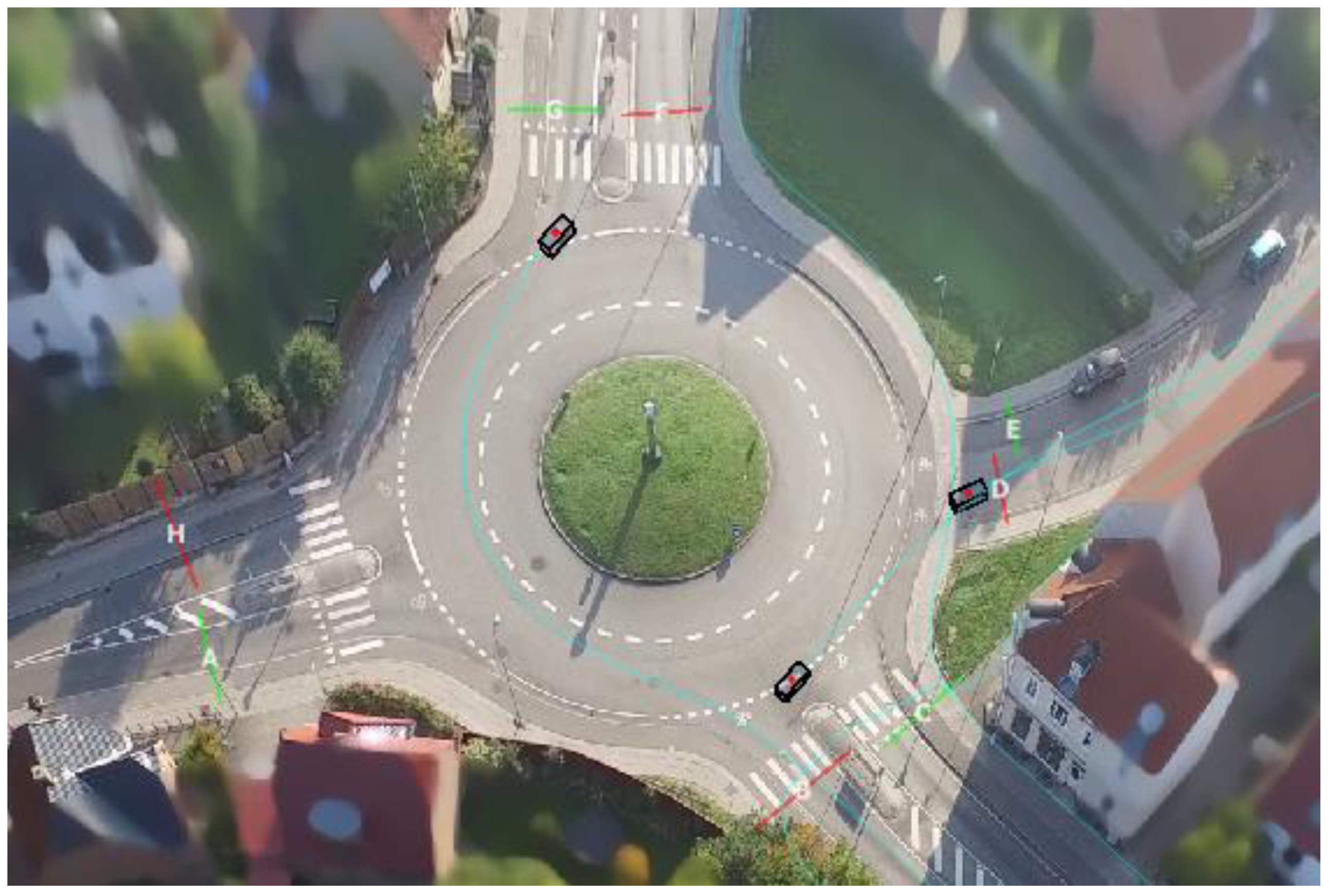
Figure 9.
(a) The screenshot of the Italy intersection taken from Google Maps [39] (Coordinates: 43.839917, 13.019667). (b) The screenshot of the Denmark A intersection taken from Google Maps [39] (Coordinates: 55.406289, 11.341097). (c) The screenshot of the Denmark B intersection taken from Google Maps [39] (Coordinates: 55.858421, 9.824669.

Figure 10.
The vehicle trajectories marked in light blue and target maneuver shown in yellow for Italy dataset.
Figure 10.
The vehicle trajectories marked in light blue and target maneuver shown in yellow for Italy dataset.

Figure 11.
(a) Three frames taken from the video sequence for car ID 57, which performs the chosen maneuver successfully in light traffic conditions. (b) Five frames taken from the video sequence for car ID 1104, which performs the chosen maneuver successfully in moderate traffic conditions.
Figure 11.
(a) Three frames taken from the video sequence for car ID 57, which performs the chosen maneuver successfully in light traffic conditions. (b) Five frames taken from the video sequence for car ID 1104, which performs the chosen maneuver successfully in moderate traffic conditions.

Figure 12.
Illustration of a typical LSTM network with associated layers.

Figure 13.
The (a) loss and (b) accuracy for the model at each training epoch for the architecture that gave the best results for Italy dataset.
Figure 13.
The (a) loss and (b) accuracy for the model at each training epoch for the architecture that gave the best results for Italy dataset.

Figure 14.
Cross-validation curves the model which gave best results for (a) Denmark-A dataset and (b) Denmark-B dataset.
Figure 14.
Cross-validation curves the model which gave best results for (a) Denmark-A dataset and (b) Denmark-B dataset.


Table 1.
Network architecture and hyper parameters for the Italy Intersection.
| Feature Name | Value | |
|---|---|---|
| Architecture | Layer 1 | LSTM (10, activation = ‘relu’, input shape = (100,12), return_sequences = True)) |
| Layer 2 | Dropout (0.2) | |
| Layer 3 | Batch Normalization | |
| Layer 4 | Dense (100, activation = ‘softmax’) | |
| Layer 5 | Dropout (0.2) | |
| Layer 6 | Time Distributed (Dense(2)) | |
| Optimizer | Adam (learning rate = 0.01, beta_1 = 0.9, beta_2 = 0.999, epsilon = 1 × 10⁻⁸, decay = 0.00) | |
| Loss Function | Mean Squared Error | |
| Batch Size | 2 | |
| Epochs | 50 | |
| Sequence Length | 100 | |
Table 2.
Network Architecture and hyper parameters for the Denmark-A.
| Feature Name | Value | |
|---|---|---|
| Architecture | Layer 1 | LSTM (10, activation = ‘tanh’, input shape = (100,12), return_sequences = True)) |
| Layer 2 | Dropout (0.4) | |
| Layer 3 | (LSTM(10, activation = ‘relu’, input_shape = (100,12), return_sequences = True) | |
| Layer 4 | Time Distributed (Dense(2)) | |
Table 3.
Network Architecture and hyper parameters for the Denmark-B.
| Feature Name | Value | |
|---|---|---|
| Architecture | Layer 1 | LSTM (10, activation = ‘relu’, input shape = (100,12), return_sequences = True)) |
| Layer 2 | Dropout (0.2) | |
| Layer 3 | Batch Normalization | |
| Layer 4 | Time Distributed (Dense(2)) | |
Table 4.
Network cross validation results summary.
| Intersection | Training | Validation | ||
|---|---|---|---|---|
| Accuracy | Loss | Accuracy | Loss | |
| Italy | 0.8148 | 0.0133 | 0.7517 | 0.0116 |
| Denmark A | 0.9925 | 0.0040 | 0.9445 | 0.0059 |
| Denmark B | 0.9591 | 0.1059 | 0.9345 | 0.0660 |
© 2019 by the authors. Licensee MDPI, Basel, Switzerland. This article is an open access article distributed under the terms and conditions of the Creative Commons Attribution (CC BY) license (http://creativecommons.org/licenses/by/4.0/).
Share and Cite
MDPI and ACS Style
Inder, K.; De Silva, V.; Shi, X. Learning Control Policies of Driverless Vehicles from UAV Video Streams in Complex Urban Environments. Remote Sens. 2019, 11, 2723. https://doi.org/10.3390/rs11232723
AMA Style
Inder K, De Silva V, Shi X. Learning Control Policies of Driverless Vehicles from UAV Video Streams in Complex Urban Environments. Remote Sensing. 2019; 11(23):2723. https://doi.org/10.3390/rs11232723
Chicago/Turabian StyleInder, Katie, Varuna De Silva, and Xiyu Shi. 2019. "Learning Control Policies of Driverless Vehicles from UAV Video Streams in Complex Urban Environments" Remote Sensing 11, no. 23: 2723. https://doi.org/10.3390/rs11232723
Note that from the first issue of 2016, this journal uses article numbers instead of page numbers. See further details here.