Theoretical Evaluation of Anisotropic Reflectance Correction Approaches for Addressing Multi-Scale Topographic Effects on the Radiation-Transfer Cascade in Mountain Environments

Abstract

Research involving anisotropic-reflectance correction (ARC) of multispectral imagery to account for topographic effects has been ongoing for approximately 40 years. A large body of research has focused on evaluating empirical ARC methods, resulting in inconsistent results. Consequently, our research objective was to evaluate commonly used ARC methods using first-order radiation-transfer modeling to simulate ASTER multispectral imagery over Nanga Parbat, Himalaya. Specifically, we accounted for orbital dynamics, atmospheric absorption and scattering, direct- and diffuse-skylight irradiance, land cover structure, and surface biophysical variations to evaluate their effectiveness in reducing multi-scale topographic effects. Our results clearly reveal that the empirical methods we evaluated could not reasonably account for multi-scale topographic effects at Nanga Parbat. The magnitude of reflectance and the correlation structure of biophysical properties were not preserved in the topographically-corrected multispectral imagery. The CCOR and SCS+C methods were able to remove topographic effects, given the Lambertian assumption, although atmospheric correction was required, and we did not account for other primary and secondary topographic effects that are thought to significantly influence spectral variation in imagery acquired over mountains. Evaluation of structural-similarity index images revealed spatially variable results that are wavelength dependent. Collectively, our simulation and evaluation procedures strongly suggest that empirical ARC methods have significant limitations for addressing anisotropic reflectance caused by multi-scale topographic effects. Results indicate that atmospheric correction is essential, and most methods failed to adequately produce the appropriate magnitude and spatial variation of surface reflectance in corrected imagery. Results were also wavelength dependent, as topographic effects influence radiation-transfer components differently in different regions of the electromagnetic spectrum. Our results explain inconsistencies described in the literature, and indicate that numerical modeling efforts are required to better account for multi-scale topographic effects in various radiation-transfer components.

1. Introduction

Remote-sensing science and technology is essential for studying and understanding the complexities associated with bio-physical/geophysical parameters and landscape dynamics [1,2]. This is especially the case in mountain environments where climate and tectonic forcings govern topography, high-magnitude surface processes, rapid environmental change and geohazards [3,4,5,6]. The inherent coupling of atmospheric, surface and tectonic processes highlights the complexity associated with mountain geodynamics, and the need for quantitative information about surface parameters, process rates and resource availability. Due to logistic, geopolitical, geohazard and physical limitations associated with fieldwork in many mountains, remote sensing represents the most effective approach for producing spatiotemporal quantitative and thematic information [7].

Remote sensing of mountain environments, however, is notoriously difficult, as multi-scale topographic effects govern the anisotropic nature of the radiation-transfer cascade (RTC) including atmospheric scattering, irradiance components, and surface reflectance [1,8]. Research indicates that it is essential to address the anisotropic nature of spectral variation caused by various radiation-transfer parameters that are strongly controlled by topographic effects [1].

Anisotropic-reflectance correction (ARC) research has been ongoing for about 40 years, e.g., [9,10,11,12,13]. Numerous approaches to ARC have been characterized as: (1) spectral-feature extraction methods; (2) statistical-empirical methods; (3) semi-empirical methods; and (4) radiation-transfer modeling [14,15]. The most frequently utilized methods from the first three categories can all be considered empirical in nature, as proxy parameters are used as surrogates for representing radiation- transfer parameters [1]. Furthermore, they are popular and have been compared to each other in various environments, because researchers and practitioners do not usually have access to spatiotemporal data, information and parameters that are required by more rigorous radiation-transfer models.

Commonly used empirical ARC methods used in comparative studies include the Statistical-Empirical Correction, B-Correction, Variable Empirical Coefficient Algorithm, Cosine Correction, C-Correction, Soil-Canopy Correction, SCS+C Correction, and Minnaert Correction. These and other approaches can be utilized based on variations in computing parameters using stratification of topography and land cover conditions in an attempt to optimize results. Given that these parameterization schemes are simplistic and cannot account for topographic anisotropy and the anisotropic nature of irradiance and reflectance, evaluation of these methods is subject to substantial uncertainties. An array of assumptions, exclusion of significant RTC parameters, and inconsistent results regarding best methods and parameterization schemes [16,17,18] strongly suggest that these ARC methods are not being adequately evaluated, given that the nature-of-the-problem is fundamentally a radiometric calibration issue.

Fundamental issues related to the complexity of the problem include the following: (1) Can ARC methods be used to produce reliable quantitative surface parameters? This will require the magnitude of surface reflectance to be valid given the viewing geometry. (2) Can ARC methods be used to process entire scenes of imagery? This will require that methods can address spatial variations in solar geometry, topographic geometry and land cover conditions. (3) Can various methods account for wavelength dependence of topographic effects? (4) Can they account for multi-scale topographic effects? (5) To what degree are methods or approaches dependent upon sensor characteristics? (6) Can they account for landscape complexity, or only work for homogeneous land cover conditions? (7) To what degree are various methods influenced by the Lambertian assumption or by the bidirectional reflectance distribution function (BRDF)? (8) Do these methods result in information compression which may be interpreted as a reduction in topographic effects? These issues have not been adequately addressed by comparative studies, although it is assumed that different methods work better in different mountain environments [16,18].

Consequently, our overall research objective was to utilize radiation-transfer modeling to improve our understanding of ARC issues by evaluating commonly used empirical methods. We generated a first-order approximation of the RTC over the Nanga Parbat Himalaya, Pakistan, and produced spectrally simulated ASTER satellite imagery. The Nanga Parbat massif is ideally suited to investigate issues associated with topographic effects and reflectance variations, as it exhibits extreme relief, the full range of slope and slope-azimuth angles, extreme spatial variability in morphometric properties including topographic shielding, and a wide variety of surface composition and land cover classes [19,20]. Specifically, we accounted for Earth–Sun orbit dynamics, atmospheric absorption and scattering, direct- and diffuse-skylight irradiance, land cover spatial structure, and surface biophysical variations in order to evaluate widely utilized empirical ARC methods for their ability to accurately account for multi-scale topographic effects, and adequately predict the magnitude and spatial variation of surface reflectance. In our research, multi-scale topographic effects were defined to be morphometric (morphology of the topography) constraints and parameters that partially govern radiation-transfer parameters. The analysis of the topography and the generation of topographic parameters and RT parameters were scale dependent with respect to direction and distance (i.e., multi-scale). It was not the purpose of this research to evaluate the influence of sensor-system characteristics on topographic-correction methods, as spatial, spectral and radiometric sensitivity also governs the variance structure in imagery. Limitations of this study include utilizing the Lambertian assumption for surface reflectance, and not accounting for the surface BRDF and the adjacent-terrain irradiance.

2. Background

2.1. Radiation-Transfer Cascade

The ARC problem requires addressing the RT components of the RTC. Specifically, the spatial, temporal, and spectral dimensions of numerous RTC parameters must be accounted for. This includes orbital, solar, atmospheric, topographic, surface composition and sensor-system characteristics.

Solar geometry variations are strongly controlled by orbital dynamics, as orbital parameters such as eccentricity, obliquity, and longitude-of-perihelion govern the Earth–Sun distance, solar declination, and solar-zenith and -azimuth angles [21,22]. The magnitude of the exoatmospheric irradiance at the top of the Earth’s atmosphere ($E^0$,[W m${}^{-2}\mathsf{\mu }$m${}^{-1}$]) is a function of the spectral exitance of the sun and the Earth–Sun distance. The atmosphere attenuates the solar beam irradiance via gaseous absorption and molecular and aerosol scattering [22,23]. Atmospheric processes are highly wavelength dependent and controlled by spatiotemporal variations in various atmospheric constituents, e.g., aerosols, water vapor; [22,24].

Atmospheric transmittance accounts for the primary constituents, such that the total downward and upward transmittance ($T^{\downarrow \uparrow }$) is represented as [25]:

$$T^{\downarrow \uparrow }({\theta }_s,\lambda )=T_r({\theta }_s,\lambda )T_a({\theta }_s,\lambda )T_g({\theta }_s,\lambda )T_o({\theta }_s,\lambda )T_w({\theta }_s,\lambda ),$$

(1)

where $T_r$ represents transmittance due to Rayleigh scatter, $T_a$ is transmittance due to aerosol scattering, $T_g$ is transmittance due to primary gas absorption, $T_o$ is transmittance due to ozone absorption, $T_w$ is transmittance due to water vapor absorption, ${\theta }_s$ is the solar-zenith angle (${\theta }_v$ should be substituted for ${\theta }_s$ for upward transmittance; ${\theta }_v$ is the sensor zenith-viewing angle), and $\lambda$ is the wavelength of light. The total atmospheric transmittance is a function of the total optical depth of the atmosphere that is related to the hypsometry of the topography, such that variations in topographic relief can cause mesoscale variations in the atmospheric optical depth and volumetric scattering of radiation. Many ARC investigations do not account for this topographic effect by applying adequate atmospheric correction procedures, although atmospheric–topographic coupling must be accounted for [1].

Various other topographic effects govern the surface irradiance (E) such that [15]:

$$E(\lambda )=E_b(\lambda )+E_d(\lambda )+E_t(\lambda ),$$

(2)

where $E_b$ represents the direct-beam irradiance from the Sun, $E_d$ represents the diffuse-skylight irradiance given atmospheric scattering, and $E_t$ is the adjacent-terrain irradiance given the irradiance scattered from the surrounding terrain. Each irradiance component is partially regulated by the atmosphere and by multi-scale topographic effects, such that it is very difficult to address topographic effects without accounting for the coupled influence of the atmosphere [26]. These components should be accounted for in mountain environments, as they can significantly influence spectral variability in satellite imagery [8].

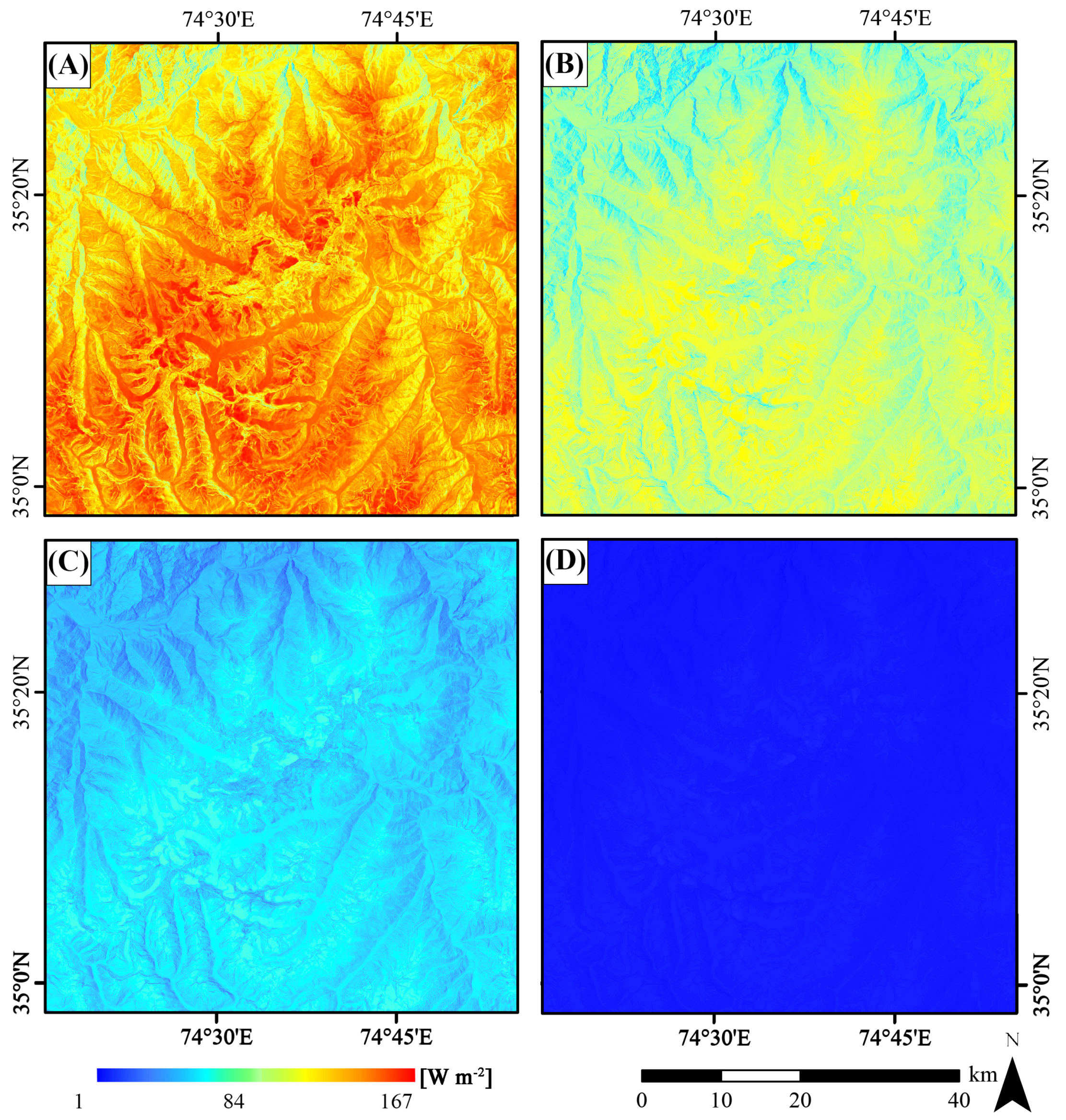
2.1.1. Direct Irradiance

The direct-beam irradiance is the dominant irradiance component [8]. It is strongly controlled by local and meso-scale topographic effects. The parameterization scheme for an exact computation of this RTC parameter is:

$$E_b(\lambda )=E^0(\lambda )T^{\downarrow }cosiS,$$

(3)

where $E^0$ is the exoatmospheric irradiance, which is modified by the Earth–Sun distance correction factor, $T^{\downarrow }$ is the downward total transmittance, $cosi$ is the cosine of the incidence angle (i), and S is a binary coefficient that accounts for cast shadows being present ($S=0.0$) or absent ($S=1.0$) on the landscape. The total transmittance can be computed from Equation (1). Numerous other atmospheric constituents can be accounted for using various atmospheric-correction models (e.g., 6S and MOTRAN). Depending upon the climatic and tectonic setting that governs erosion, uplift and relief production, atmospheric transmittance may or may not be a significant RTC parameter for ARC. It is not usually accounted for in representing $E_b$, because $cosi$ is used as a proxy in most empirical ARC methods.

It is necessary to address local topographic effects that account for the relationship between the solar and terrain geometry. Specifically, the incidence angle of illumination (i) between the sun and normal to the ground surface is defined as:

$$cosi=cos{\theta }_{s}cos{\theta }_t+sin{\theta }_{s}sin{\theta }_{t}cos\left({\varphi }_s-{\varphi }_t\right),$$

(4)

where ${\theta }_s$ is the apparent solar-zenith angle that accounts for altitude variations and atmospheric refraction given the atmospheric temperature and pressure profiles, ${\theta }_t$ represents the terrain slope angle, ${\varphi }_s$ is the solar-azimuth angle, and ${\varphi }_t$ is the terrain slope-azimuth angle. Calculation of $cosi$ is possible with the use of a digital elevation model (DEM), and negative values must be corrected to $0.0$. The solar geometry is governed by orbital parameters that vary over time. The magnitude of variation increases over larger time periods. Most researchers do not compute the solar geometry for every pixel, thereby assuming the small-angle approximation, using one estimate for these parameters obtained from imagery for the entire scene or subscene. Nevertheless, as solar geometry is a function of location and time, the solar geometry varies for each pixel in a scene. It is unclear to what degree the small-angle approximation governs the accuracy of ARC efforts, as researchers usually do not evaluate full scenes of satellite imagery.

Finally, the meso-scale relief structure of the topography, coupled with temporally-dependent solar geometry, governs the presence of cast shadows on the landscape. Ray-tracing algorithms can be used to account for this influence on $E_b$ [27,28,29,30]. It should be noted that this parameter is independent of the computation of $cosi$, and many studies do not account for it. It may or may not be an issue in ARC investigations depending upon the time of image acquisition and the magnitude of relief in the direction of the solar azimuth.

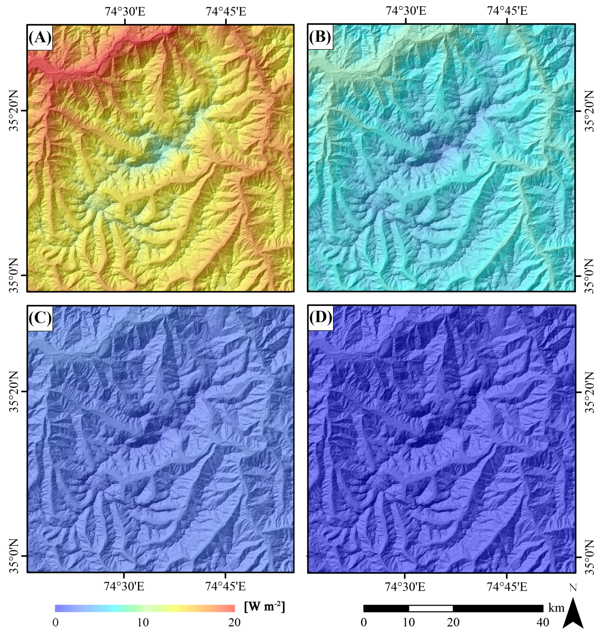
2.1.2. Diffuse-Skylight Irradiance

Atmospheric scattering will produce a hemispherical source of irradiance that contains isotropic and anisotropic components [8,31]. The anisotropic nature of $E_d$ has been the largest source of error associated with estimating this component, as it is governed by circumsolar brightening due to forward scattering of aerosols, and horizontal brightening due to multiple Rayleigh scattering [31]. An approximation model assumes that:

$$E_d(\lambda )=E_r(\lambda )+E_a(\lambda )+E_g(\lambda ),$$

(5)

where $E_r$ is the Rayleigh-scattering component, $E_a$ is the aerosol-scattering component, and $E_g$ is the ground/sky-backscattering component caused by multiple interactions between the ground surface and the atmosphere [1,8,24]. One can account for single-scattering or a multiple-scattering Rayleigh atmosphere. The single-scattering albedo is required to account for aerosol scattering which is a function of both wavelength and humidity. Aerosol type and models such as rural, urban, maritime or tropospheric can also be accounted for [24]. Finally, the ground-backscattering component can be modeled by accounting for the zonal-ground reflectance from the direct irradiance, the reflectance from the diffuse irradiance, and the overall sky reflectance [24].

To account for the diffuse irradiance for every pixel, numerous topographic effects must be accounted for and computed. Proy et al. [8] provided the computation solution such that:

$$E_d(\lambda )={\int }_{{\varphi }_i=0}^{2\pi }{\int }_{{\theta }_i=0}^{\pi /2}{L}^{\downarrow }\left({\alpha }_s,{\theta }_i,{\varphi }_i\right)cosIsin{\theta }_{i}d{\theta }_{i}d{\varphi }_i,$$

(6)

where $L^{\downarrow }$ is the downward radiance from incident directions ${\theta }_i$ and ${\varphi }_i$, which are the zenith and azimuth angles of the incident energy from the hemisphere, respectively; ${\alpha }_s$ is the solar elevation angle (${\alpha }_s=\pi /2-{\theta }_s$); and I is the incidence angle of the direction defined by hemisphere and terrain geometry, similar to Equation (4) using incident geometry.

Such an exact computation is computationally intensive given that $E_d$ is wavelength dependent, and hemispherical-topographic shielding must be accounted for. Multiple approaches to account for topographic shielding are based on the computation of a maximum relief angle ${\theta }_{max}$ for ${\varphi }_i$, e.g., [27,32]. The so-called skyview-factor coefficient is usually multiplied by estimates of diffuse irradiance for a horizontal surface to compute $E_d$. Many researchers do not utilize this parameter due to computational intensity, but estimate it based on the slope angle, e.g., [33,34]. It is rare for investigators to account for both $cosI$ and ${\theta }_{max}({\varphi }_i)$, thereby accounting for local and meso-scale topographic effects.

2.1.3. Adjacent-Terrain Irradiance

The aforementioned irradiance components and surface reflectance interact with the surrounding terrain geometry to produce the $E_t$ irradiance component. Numerous researchers have indicated that this component must be accounted for in mountains due to snow, vegetation and steep slopes [8,33,35]. It is an extremely complicated parameter to compute, as it is governed by numerous multi-scale topographic effects and surface anisotropic-reflectance conditions. A first-order approximation to $E_t$ was formulated by Proy et al. [8], assuming Lambertian reflectance. It is rarely accounted for in empirical ARC studies.

Its exact computation is:

$$L\left({\theta }_i^e,{\varphi }_i^e,{\theta }_v^e,{\varphi }_v^e,\lambda \right)={\rho }_{brdf}\left({\theta }_i^e,{\varphi }_i^e,{\theta }_v^e,{\varphi }_v^e,\lambda \right)E(\lambda ),$$

(7a)

$$E_t(\lambda )={\int }_{{\varphi }_i=0}^{2\pi }{\int }_{{\theta }_i=0}^{\pi }L\left({\theta }_i^e,{\varphi }_i^e,{\theta }_v^e,{\varphi }_v^e,\lambda \right)T_t^{\downarrow \uparrow }({\theta }_v^e,\lambda )cos{I}_t{S}_{t}d{\theta }_{i}d{\varphi }_i,$$

(7b)

where L is the surface-reflected radiance coming from the effective incident direction, ${\rho }_{brdf}$ is the surface BRDF, ${\theta }_i$ is the incident vertical-hemispherical zenith angle to account for terrain radiance above and below a pixel location, $T_t^{\downarrow \uparrow }$ is the atmospheric transmittance given the optical depth of the atmosphere due to relief and propagation zenith angle through the atmosphere (${\theta }_v$) between two locations, $I_t$ represents the terrain-incidence angle given the influence of the local terrain geometry in relation to the incident directional geometry, and $S_t$ represents terrain blocking of the surface radiance between any two points of the surrounding terrain. The superscript e represents the effective zenith and azimuth angles that account for the influence of the terrain slope and slope-azimuth angles on the incident (${\theta }_i^e,{\varphi }_i^e$) and viewing geometry (${\theta }_v^e,{\varphi }_v^e$) of the surface BRDF compared to a horizontal surface. The computation of $E_t$ should account for the terrain conditions extending out to approximately 5 km from each pixel location [8]. Another complicating factor is that each pixel exhibits a unique BRDF, as topography and varying land cover structure and biophysical properties govern the BRDF [36,37,38].

Most empirical ARC investigations do not adequately account for $E_t$, as they assume Lambertian reflectance, insignificant atmospheric attenuation, and do not iteratively compute estimates of $E_t$ over time ($E_t$ is partially governed by $E_t$). Such assumptions are not valid in many mountain environments, as steep slopes and highly variable biophysical properties caused by high-magnitude surface processes, create anisotropic reflectance conditions and extreme relief [11,35,39,40,41,42,43,44,45]. Furthermore, topographic effects on the surface BRDF are not fully understood, although we know that the viewing geometry changes for every pixel, given variations in terrain slope and slope-azimuth angles [1].

2.1.4. Bi-Directional Reflectance Distribution Function

The characteristics of surface-reflectance properties can range between diffuse and specular [1,46]. A diffuse or Lambertian surface reflects radiation in all directions equally, and is considered an isotropic reflector. We know, however, that this assumption is not valid in mountains, and the surface BRDF should be accounted for to enable effective ARC [1]. The BRDF is used to describe the anisotropic nature of surface reflectance characteristics. It is a scattering function and can theoretically describe anisotropic reflectance given all input–output angles. It is characterized as:

$${\rho }_{brdf}({\theta }_i^e,{\varphi }_i^e,{\theta }_v^e,{\varphi }_v^e,\lambda )=\frac{L(\lambda )}{E(\lambda )}.$$

(8)

The effective illumination (${\theta }_i^e,{\varphi }_i^e$) and viewing directions (${\theta }_v^e,{\varphi }_v^e$) are a function of ${\theta }_s$, ${\varphi }_s$, ${\theta }_t$, ${\varphi }_t$, ${\theta }_v$, and ${\varphi }_v$. Consequently, the topography has a significant effect on the BRDF [1]. The BRDF, however, is difficult to measure accurately, and, in practice, the bidirectional reflectance factor (BRF) is commonly used [1,47]. The application of different BRDF models in ARC studies has been relatively limited, and most studies utilize semi-empirical models because they can be fit to measured data [1]. These models are very flexible and account for a geometric component due to land cover structure and a diffuse volume component. Empirical coefficients can be used to determine the relative strength of these two scattering characteristics. The importance of topographic effects on the BRDF in ARC research cannot be overstated. They partially govern $E_d$, $E_t$, L, and $L_p$ (the ground component of additive-path radiance). Clearly, empirical ARC methods are too simplistic to account for the spectral variation of numerous radiation-transfer parameters that are part of the RTC.

2.2. ARC

The strong influence that topography has on spectral response as measured by satellite-scanner systems in rugged terrain has long been recognized, e.g., [48]. Various approaches have been introduced in an attempt to reduce or remove these effects. Nevertheless, a topographic-correction method has not emerged that is consistently superior in all cases [16,18]. In addition, commonly applied topographic-correction methods do not provide a fully comprehensive ARC solution. Topographic-correction approaches can be organized into three categories: spectral-feature extraction methods, empirical modeling, and radiation-transfer modeling [49,50,51]. Empirical methods can be divided into those based on a Lambertian assumption of surface reflectance and those based on a non-Lambertian assumption. The following background section discusses empirical topographic-correction approaches, as these represent the most commonly used methods and were evaluated in this study.

Empirical Corrections

In contrast to spectral-feature extraction methods such as band ratios, which involve a linear transformation of spectral values without incorporating ancillary data [52,53], empirical topographic corrections utilize slope and slope-azimuth angles computed from a DEM, and attempt to simulate the direct-beam irradiance using the cosine of the incidence angle. Some empirical methods rely on using statistical analysis to adjust spectral response values based on mean spectral values calculated for shaded and sunlit slopes, e.g., [54], for entire images or for selected cover types. Other methods use regression analysis to derive coefficients in an attempt to represent physical properties such as the diffuse-skylight irradiance, or the BRDF of surface cover types. These methods are all essentially empirical, as their calculations and generation of coefficients depend on the specific spatial and temporal characteristics of individual study areas (e.g., slope and slope azimuth, solar geometry, land cover).

Perhaps the most often used, and reportedly successful method adjusting spectral response based on mean values is the Statistical-Empirical Correction (SEC; see Equation (19b)) [55,56]. The SEC equation has also been referred to as the Teillet regression [14,18,57]. The SEC is a statistically based model that assumes that the mean spectral values on a horizontal surface are equal to those on tilted surfaces [58]. A number of authors have indicated the superior performance of the SEC when comparing topographic-correction algorithms, e.g., [59,60,61,62]. As with other topographic correction methods reported in the literature, different algorithms have been used to represent the SEC, e.g., [13,51,63].

The variable empirical coefficient algorithm (VECA) method (see Equation (22c)) was introduced by Gao and Zhang [14] and has been favorably compared to other topographic-correction methods [12,62]. The VECA was developed to overcome some of the challenges of applying more complex correction methods [14]. Similar to the SEC, the VECA algorithm adjusts the reflectance of pixels on an inclined surface based on a linear regression, incorporating $cosi$, and using the mean radiance values for pixels on horizontal and tilted surfaces [14,57,62]. The B-correction as proposed by Vincini et al. [64] can be calculated using either a linear isotropic (BLC, see Equation (20c)) or non-linear anisotropic form (BNC, see Equation (21b)). According to Gao and Zhang [14], the VECA and B-corrections proved to be capable of removing topographic effects in a Landsat ETM+ image, although the success of the algorithms were wavelength dependent and they each performed better in different bands [14].

If the Lambertian assumption accurately describes a surface, then topographic correction can be accomplished using a simple Cosine Correction (COSC, see Equation (23)) [39]. Numerous studies have found that the Cosine Correction overcorrected for local topographic effects, particularly on northern slopes, e.g., [65,66,67]. These overcorrections have been attributed to only $E_b$ being accounted for, as weakly illuminated areas can actually receive a significant amount of $E_d$ [56,68], and the inability of the Cosine Correction to account for BRDF variations of land cover surfaces [65].

Teillet et al. [55] modified the Cosine Correction with an additive term C (CCOR, see Equation (24c)) that the authors stated may emulate the effect of indirect illumination, although, the analogy is not exact. The C coefficient has been used to prevent the overcorrection of images [69], and notwithstanding the ambiguity of the original authors, has often been credited with accounting for $E_d$, e.g., [16,26,61]. As a Lambertian model, the C-Correction does not take into account the BRDF of land cover features. Results from applying the C-Correction in studies comparing topographic correction methods have been mixed, with the correction performing well in some studies, e.g., [61,63], and not as well in others [51,70]. For example, Fan et al. [57] found the C-Correction to be theoretically and empirically inappropriate for forested terrain.

Topographic-correction methods have been applied to correct spectral-reflectance values for single and multiple cover types using sun–terrain–sensor (STS) geometry. To improve the representation of the geotropic nature of trees, Gu and Gillespie [71] introduced a method based on sun–canopy–sensor (SCS) geometry, which incorporates slope into the Cosine Correction (see Equation (25)) [54]. Application of the SCS method has often resulted in overcorrection, e.g., [14,69,72]. To address overcorrections, Soenen et al. [72] introduced the SCS+C method (see Equation (26)) incorporating the additive term C to attempt to account for $E_d$, in a similar fashion to how the C coefficient adjusts the Cosine Correction [69]. Generally, the SCS+C correction has outperformed the SCS method, e.g., [18,69,73].

A commonly applied non-Lambertian topographic correction method that attempts to incorporate a representation of land cover BRDF is the Minnaert Correction (GMC, see Equation (27)). According to Smith et al. [39], the Minnaert constant k [74] is related to surface roughness. Calculation of k varies based on combinations of slope, slope azimuth and land cover, e.g., [9,11]. A global Minnaert k value is calculated per band using reflectance values from multiple cover types across an entire image, e.g., [75]. However, calculating the empirical coefficients C and k over large areas is problematic due to their dependence on land cover variation [57,61,62]. Attempts have been made to calculate k for land cover classes, e.g., [19], and using stratifications based on slope, slope azimuth, and land cover, such as the Modified Minnaert [16] and the Pixel-Based Minnaert (PMC; see Equation (28)) [76]. Minnaert corrections do not incorporate contributions from $E_d$ and $E_t$ [9].

2.3. ARC Evaluation

Effective topographic correction should result in a reduction of spectral variation globally across an image caused by multi-scale topographic effects, and an increase in local spectral variation in poorly illuminated areas due to biophysical property or land cover variations [15]. The performance of topographic-correction methods is dependent upon evaluation strategies [18]. Various approaches have been used to evaluate the effectiveness of topographic-correction methods; however, evaluation results are difficult to compare and there is still not a simple and objective approach for evaluating correction effectiveness [63]. Diagnostic methods generally fall within four categories according to a review of recent articles comparing topographic-correction methods. These categories include visual assessment, statistical methods, classification accuracy, and comparisons to simulated/synthetic images.

The most common and usually initial method for evaluating topographically-corrected images is a visual assessment. Visual assessments have been employed since correction methods were first attempted, e.g., [55] and continue to be applied, e.g., [13]. Usually singular images are evaluated, although image bands have been draped across DEMs to create an orthographic image for interpretation [60]. Even though visual assessment is used extensively as an evaluation method [16], it is fundamentally a subjective approach that is based heavily on the experience and skill of the analyst, e.g., [57] and must be combined with a quantitative assessment [62]. Visual assessment results may differ markedly from quantitative evaluations. For example, corrected images can appear similar and be statistically different [16,60]. In addition, variance compression may occur during topographic correction, which can visually be interpreted as a reduction of topographic effects [19].

Univariate and multi-variate statistical analysis methods have been applied towards evaluating the effectiveness of topographic-correction approaches including intraclass interquartile range reduction [63] and comparisons with in-situ observations of spectral reflectance [70]. Two of the most common methods for comparing imagery before and after correction include assessing a reduction in standard deviation (SD), and comparing the coefficient of variation (CV). Evaluations of the reduction of SD have been made across images [50] or within the same cover types on different slopes and aspects [18,61,73]. Ideally, an effective correction will maintain the mean of the original band or cover type and the SD will be reduced [50,66]. Essentially, these as well as other statistical diagnostic methods are testing for an increase in the homogeneity of reflectance values after correction, e.g., [50,62]. It is not valid, however, to presume spectral homogeneity across an image with different land covers or within the same land cover, such as vegetation with different stand ages, understory, or crown canopies, which can result in different spectral responses, e.g., [18]. Additionally, effective corrections do not always substantially change standard deviations and histogram distributions of imagery data [60]. Therefore, these methods may not account for the spatially-dependent variance structure across an image or within some land cover types.

A range of inferential-statistical methods have been used to evaluate the effectiveness of topographic corrections such as the univariate analysis of variance [69], multivariate analysis of variance [77], and homogeneity of variance [11]. Geo-statistical analyses, such as semi-variogram analysis [19], have also been applied. Perhaps the most common statistical method for evaluating pre- and post-corrected imagery is based on a linear regression (coefficient of determination, $r^2$) with the spectral values represented as the dependent variable and cos i as the independent variable, e.g., [39]. The spectral values have been represented as digital numbers (DN), e.g., [56,59,60,73] and radiance values, e.g., [14,63,70]. The assumption is that an effective correction will result in the removal of reflectance dependence on $cosi$. However, in areas where land cover distribution is affected by slope and aspect [61], this assumption is not valid [63]. In mountainous areas with large elevation gradients, spatial patterns of land cover will be dependent upon topographic variables, and a residual correlation would be expected between reflectance values and $cosi$ after correction [18,63]. Additionally, $cosi$ accounts only for local topography and does not incorporate multi-scale topographic effects [15]. Decorrelation of the linear regression is not sufficient to indicate a successful correction [57].

Two of the primary purposes for performing topographic corrections is to improve land cover classification [9,18,78] and biophysical parameter extraction [63]. An improvement in classification accuracy is a common method for determining the effectiveness of topographic correction. Classification methods have been evaluated such as maximum likelihood [26,50,59], artificial neural networks [50,54], and object-based classification [73]. The primary difficulty in using classification accuracy as a diagnostic method is that many factors and potential sources of error are inherent in the classification process [19,50]. Classification analysis is affected by study area characteristics, land cover types, within-class covariance, quality of reference data, sensors, DEMs, atmospheric effects and corrections, geometric corrections, classification algorithms, and topographic effects [26,57,62]. The uncertainties inherent in these factors and their various combinations make it difficult to relate quantitative classification results directly to the quality of topographic corrections, and to compare study results [26,63,79]. Classification provides an indirect evaluation [57], and is not a good indicator of topographic-correction effectiveness [19,50,57,79].

Given the shortcomings and difficulties in comparing results when using traditional evaluation strategies, the development of a more standardized and objective procedure is warranted. The comparison of a corrected image to a synthetic image could provide the basis for this type of approach [18,79]. The synthetic image represents idealized radiance according to specific conditions, and can be generated representing a flat surface or incorporating topography [79]. Quantitative evaluation of the comparison between corrected and synthetic images can be undertaken using a structural-similarity index [79,80], or comparable similarity indices [63,81]. Potential drawbacks to this approach include the complicated process required for producing synthetic images [81].

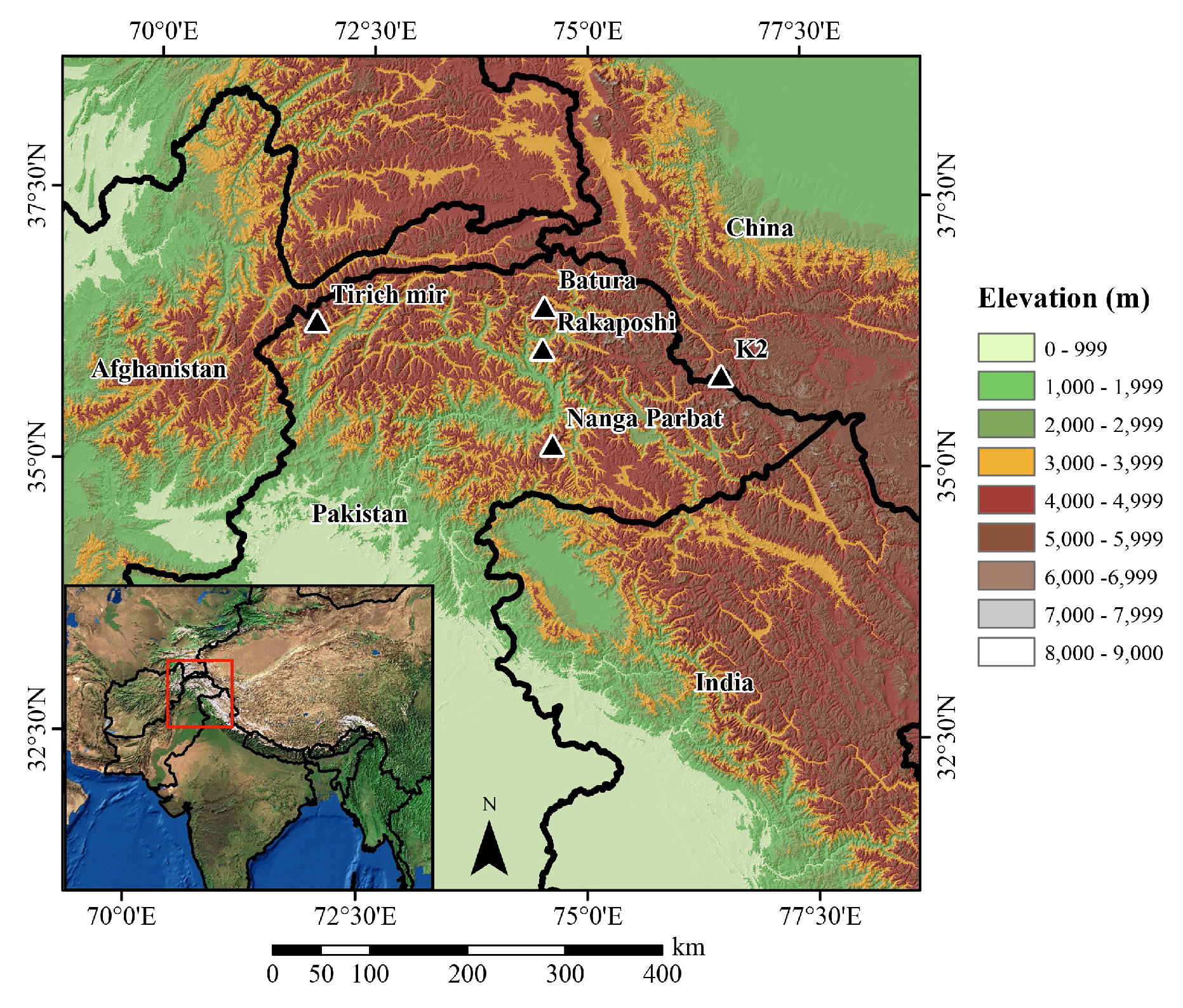
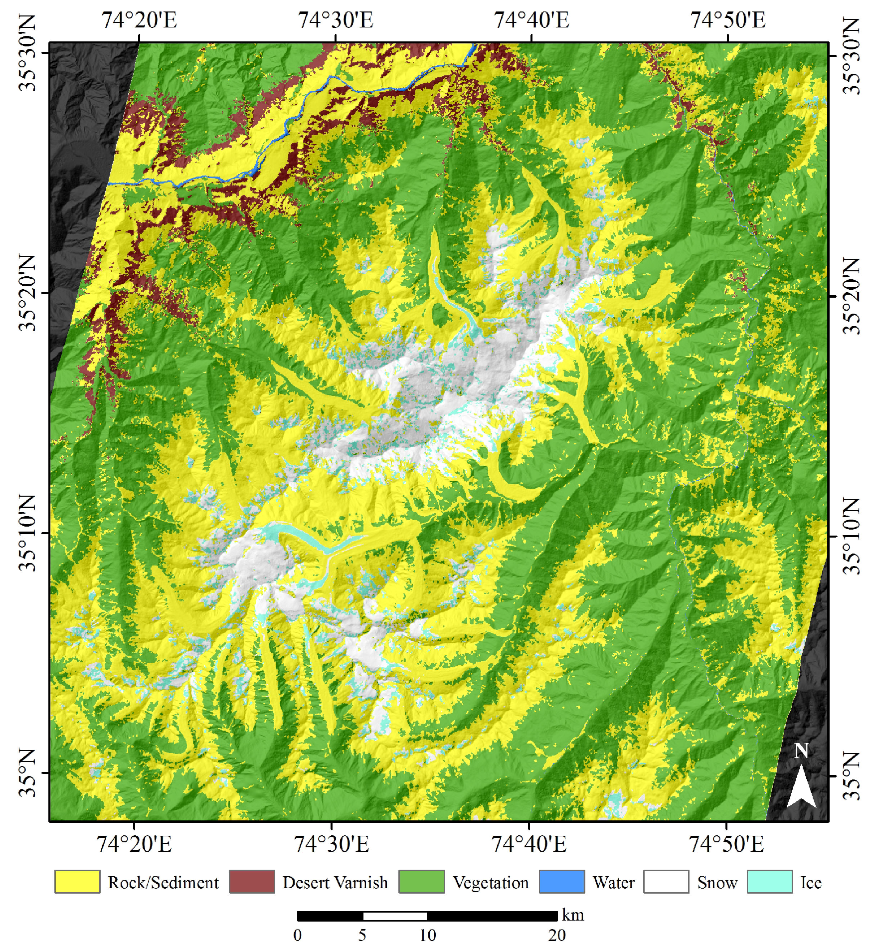
2.4. Study Area

We simulated a first-order approximation of the RTC over the Nanga Parbat, Himalaya in northern Pakistan (Figure 1). This geographic region is excellent for testing empirical-correction procedures, as it exhibits extreme relief and steep slopes due to relief production caused by high-magnitude erosion and uplift [3,20,82,83]. We specifically simulated the RTC over a 60 km × 60 km area to evaluate the ability of empirical-correction procedures to account for the spatial complexity of an entire scene of ASTER imagery.

Topographic conditions over the region are highly variable due to complex spatiotemporal surface-process dynamics [3] that are governed by climate and topographic forcing. Glaciation, rapid river bedrock incision, and ubiquitous mass movements govern the dynamic nature of the sediment fluxes, and differential denudation coupled with uplift has resulted in significant relief production [83]. Consequently, surface conditions are very spatially variable from material composition and surface/landcover structural perspectives. Such conditions dictate anisotropic-reflectance conditions. Surface-process dynamics and landcover conditions are also regulated by two climatic systems that include the westerlies and the monsoon [20,82]. For more details regarding the study area characteristics, see Bishop and Shroder [20] and Bishop et al. [3].

3. Materials and Methods

3.1. Data

The ASTER Global Digital Elevation Model Version 2 (ASTER GDEM; [84]) was utilized to represent the topography and account for several multi-scale topographic effects governing the RTC. We spectrally simulated ASTER imagery (bands 1, 2, 3 and 5) for an entire scene which accounted for a $2000\times 2000$ grid cell area centered over Nanga Parbat peak. We used a $4000\times 4000$ dataset for computation of the cast shadows and topographic-shielding parameters to avoid edge effects. This study also utilized ASTER satellite imagery acquired over the area on 13 September 2004, to provide information about the spatial structure of the land cover characteristics that are described in greater detail below. Mean Exo-atmospheric irradiance values from Bird and Riordan [25] were used in simulating the RTC. Reference reflectance spectra were acquired from the United States Geological Survey Spectral Library Version 7 [85] and the ASTER Spectral Library [86].

3.2. Radiation-Transfer Modeling

We simulated ASTER multispectral imagery in order to evaluate frequently used empirical ARC methods. This involves implementing a first-order radiation-transfer model to simulate the RTC from the sun to the at-satellite sensor. We account for multi-scale topographic effects for each radiation-transfer parameter used in our simulation. Although higher-order modeling parameterization schemes can be utilized, they are not required to test and evaluate the most fundamental topographic effects, as the most common ARC methods account for only 1–3 proxy parameters representing the RTC. Furthermore, our approach permits detailed quantitative analysis of the significance of individual parameters and their wavelength dependence.

3.2.1. Exoatmospheric Irradiance and Solar Geometry

The mean exoatmospheric irradiance spectrum of Bird and Riordan [25] was modified using temporally dependent orbital parameters to compute the spatiotemporal dependent exoatmospheric irradiance spectrum ($E^0(\lambda )$). Earth–sun orbital parameters control the magnitude of $E^0$; therefore, orbital forcing must account for eccentricity (e), obliquity ($ϵ$) and other parameters such as the longitude of perihelion [21]. We used the Berger [21] amplitudes, rates and phases of trigonometric expansions to predict these orbital parameters for 15 September 2018 to compute the Earth–Sun distance (d), the distance-correction factor ($f_r$) and solar geometry at 10: local time, such that:

$$E^0(\lambda )={\overline{E}}^0(\lambda )f_{r}cos{\theta }_s,$$

(9)

where ${\theta }_s$ is the solar-zenith angle.

Orbital parameters are also required to compute the spatial variation in the solar geometry such that:

$$\delta =arcsin\left(sinϵsin{\lambda }_l\right),$$

(10)

where $\delta$ is the solar declination and ${\lambda }_l$ is the true longitude of the Earth relative to the vernal equinox.

The solar-zenith angle (${\theta }_s$) and solar-azimuth angle (${\varphi }_s$) vary for each pixel if spatial and topographic factors are accounted for. The geocentric solar-zenith angle is:

$$cos{\theta }_s=sin\phi sin\delta -cos\phi cos\delta cosH,$$

(11)

where $\phi$ is latitude, and H is the hour angle of the sun. This parameter, however, must be modified using a parallax correction to compute the apparent solar-zenith angle from the Earth’s surface given topography. Parallax correction accounts for the radius of the Earth at a particular latitude, the height relative to the ellipsoid, and the distance from the sun, and is added to the geocentric solar-zenith angle. Finally, we accounted for atmospheric-refraction correction based on the parameterization scheme of U.S. Naval Observatory and Nautical Alamanc Office [87], where we accounted for the atmospheric profile of temperature and pressure of the US standard atmosphere [88].

The solar-azimuth angle for each pixel was computed as:

$${\varphi }_s=\pi atan2(Y_s,X_s),$$

(12a)

where the sine and cosine components are computed as:

$$Y_s=\frac{\left(-cos\delta sinH\right)}{cos{\alpha }_s},$$

(12b)

and

$$X_s=\frac{\left(sin{\alpha }_{s}sin\phi -sin\delta \right)}{\left(cos{\alpha }_{s}cos\phi \right)},$$

(12c)

where ${\alpha }_s$ is the solar elevation angle. The solar-azimuth angle was then corrected for grid convergence, which is a function of latitude and the longitude of a pixel location with respect to the central meridian of the projection used (i.e., Transverse Mercator). See

Table A1. Numerical modeling parameter values used for characterizing atmospheric constituents and properties for atmospheric transmittance and path radiance components of the radiation-transfer cascade.

Description	Symbol	Value	Source
Earth–Sun Distance	R	1.005711546525589 AU	Computed
Earth–Sun Distance Correction Factor	D	0.988674032	Computed
U.S. Standard Air Pressure at Sea Level	$P_0$	1013.25 mbar	Jacobson [22]
U.S. Standard Air Temperature at Sea Level	$T_0$	288 K	Jacobson [22]
Average mass of one air molecule	$\overline{M}$	$4.8096\times {10}^{-26}\mathrm{kg}$	Jacobson [22]
Precipitable Water Vapor	W	3.4 cm	Interpolated from Leckner [89]
Ozone Standard Midlatitude	$O_3$	0.3434 atm cm	Gueymard [24]
Height of Maximum Ozone Concentration	$h_o$	22 km	Bird and Riordan [25]
Turbidity Coefficient	$\beta$	0.1	Gueymard [24]
Turbidity Coefficient	${\alpha }_1$	1.0274	Bird and Riordan [25]
Turbidity Coefficient	${\alpha }_2$	1.206	Bird and Riordan [25]
Aerosol Single-Scattering Albedo at $\lambda =0.4\mathrm{\mu }\mathrm{m}$	${\omega }_{0.4}$	0.945	Bird and Riordan [25]
Aerosol Wavelength Variation Factor	${\omega }^{\prime }$	0.095	Bird and Riordan [25]
Aerosol Asymmetry Coefficient	$k_0$	0.75141	Gueymard [24]
Aerosol Asymmetry Coefficient	$k_1$	−0.35648	Gueymard [24]
Aerosol Asymmetry Coefficient	$k_2$	0.29982	Gueymard [24]
Aerosol Asymmetry Coefficient	$k_3$	−0.081346	Gueymard [24]
Aerosol Asymmetry Coefficient	$k_4$	0.0073038	Gueymard [24]

(Appendix A) for values utilized for modeling solar geometry and

Table A2. Symbol notation.

Symbol	Unit	Description
${\alpha }_s$	[radians]	Solar elevation angle
${\overline{\rho }}_s$	unitless	Weighted sensor response surface reflectance
$\delta$	[radians]	Solar declination
$\lambda$	$[\mathsf{\mu }$m]	Wavelength of light
${\lambda }_l$	[radians]	True longitude of the Earth relative to the vernal equinox
$\omega$	unitless	Single-scattering albedo
${\varphi }_i$	[radians]	Hemisphere azimuth angle of incident energy
${\varphi }_s$	[radians]	Solar-azimuth angle
${\varphi }_t$	[radians]	Terrain slope-azimuth angle
${\varphi }_i^e$	[radians]	Effective slope-azimuth angle incident energy accounting for topographic correction
${\varphi }_v^e$	[radians]	Effective slope-azimuth viewing angle accounting for topographic correction
${\rho }_s^c$	unitless	Composite surface reflectance
${\rho }_{brdf}$	unitless	Surface BRDF
${\rho }_a$	unitless	Spectral sky reflectance of the atmosphere
${\rho }_j$	unitless	Reflectance of end-member j
${\rho }_n$	unitless	Normalized surface reflectance after topographic correction
${\theta }_{max}$	[radians]	Maximum relief angle
${\theta }_i$	[radians]	Hemisphere zenith angle of incident energy
${\theta }_s$	[radians]	Solar-zenith angle
${\theta }_t$	[radians]	Terrain slope angle
${\theta }_v$	[radians]	Viewing zenith angle
${\theta }_i^e$	[radians]	Effective zenith angle of incident energy accounting for topographic correction
${\theta }_v^e$	[radians]	Effective viewing zenith angle accounting for topographic correction
$\phi$	[radians]	Latitude
b	unitless	Snow scattering asymmetry factor
c	unitless	Contrast variance parameter for $SSI$
d	[km]	Earth–Sun distance
E	[W m${}^{-2}]$	Surface irradiance
e	[radians]	Exitance angle
$E^0$	[W m${}^{-2}$$\mathsf{\mu }$m${}^{-1}]$	Exoatmospheric irradiance
$E_a$	[W m${}^{-2}]$	Aerosol scattering irradiance component
$E_b$	[W m${}^{-2}]$	Direct-beam irradiance from the Sun
$E_d$	[W m${}^{-2}]$	Diffuse-skylight irradiance
$E_g$	[W m${}^{-2}]$	Ground/sky backscattering irradiance component
$e_j$	unitless	Error term
$E_r$	[W m${}^{-2}]$	Irradiance due to Rayleigh scattering
$E_t$	[W m${}^{-2}]$	Adjacent-terrain irradiance
$f_j$	unitless	Fraction of end-member j
$f_r$	unitless	Earth–Sun distance-correction factor
H	[radians]	Hour angle of the Sun
i	[radians]	Incidence angle
I	[radians]	Hemisphere incidence angle
$I_t$	[radians]	Adjacent terrain-incidence angle
k	unitless	Minnaert coefficient
l	unitless	Collective influence of reflectance magnitude for $SSI$
L	[W m${}^{-2}$ sr${}^{-1}$ $\mathsf{\mu }$m${}^{-1}]$	Surface radiance
$L^{\downarrow }$	[W m${}^{-2}]$	Hemispherical downward diffuse irradiance
$L^0$	[W m${}^{-2}$ sr${}^{-1}$ $\mathsf{\mu }$m${}^{-1}]$	At-satellite radiance
$L_n$	[W m${}^{-2}$ sr${}^{-1}$ $\mathsf{\mu }$m${}^{-1}]$	Surface radiance after topographic normalization
$L_p$	[W m${}^{-2}$ sr${}^{-1}$ $\mathsf{\mu }$m${}^{-1}]$	Additive path radiance
r	unitless	Pearson-Product Moment correlation coefficient
S	unitless	Binary coefficient for cast shadows
$SSI$	unitless	Structural-similarity index
$S_t$	unitless	Binary coefficient for terrain blocking
$T_a$	unitless	Transmittance due to aerosol scattering
$T_g$	unitless	Transmittance due to primary gas absorption
$T_o$	unitless	Transmittance due to ozone absorption
$T_r$	unitless	Transmittance due to Rayleigh scattering
$T_w$	unitless	Transmittance due to water vapor absorption
$T^{\downarrow }$	unitless	Total downward transmittance
$T^{\uparrow }$	unitless	Total upward transmittance
$T^{\downarrow \uparrow }$	unitless	Total downward/upward transmittance
$T_t^{\downarrow \uparrow }$	unitless	Total atmospheric transmittance due to terrain relief

(Appendix B) for explanation of symbol notation utilized throughout this paper.

3.2.2. Atmospheric Parameters

Atmospheric absorption and scattering processes account for atmospheric attenuation and the additive path-radiance components. These processes are wavelength dependent, and we simulated them from blue to short-wave infra-red wavelengths. We computed the downward and upward total transmittance parameters based on primary atmospheric constituents and processes. Specifically, they include Rayleigh scattering transmittance ($T_r$) using the parameterization scheme of Gueymard [24] that is wavelength and pressure dependent. Atmospheric pressure was computed based on the scale height of the atmosphere, which accounts for the virtual temperature, and the variation in gravitational acceleration, which is a function of latitude and altitude. Aerosol-scattering transmittance ($T_a$) was accounted for using the scheme of Bird and Riordan [25] using a rural aerosol model. Atmospheric absorption transmittance of water ($T_w$), ozone ($T_o$) and primary gases ($T_g$) were simulated using the parameterization schemes of Leckner [89]. All parameterization schemes effectively accounted for altitude variations in governing the pressure and relative optical air mass given by Kasten [90]. The atmospheric parameters used in these parameterization schemes to simulate atmospheric transmittance are listed in Table A1. Finally, the total downward ($T^{\downarrow }$) and upward ($T^{\uparrow }$) atmospheric transmittances were computed using Equation (1).

The additive path radiance ($L_p$) due to atmospheric scattering can be computed as [79]:

$$L_p(\lambda )=\frac{E^0(\lambda )cos{\theta }_s{\rho }_a(\lambda )}{\pi },$$

(13)

where ${\rho }_a$ is the sky reflectance of the atmosphere. Different sky-reflectance models exist, and we used the parameterization scheme of Gueymard [24]. It accounts for scattering in the sensor field-of-view due to Rayleigh scattering and aerosol absorption and scattering. It also accounts for the single-scattering component of the scattering flux which is dependent upon the aerosol asymmetry factor coefficients found in Table A1. For more details regarding the equations used to compute ${\rho }_a$, see Gueymard [24]. See Table A1 for all values utilized for modeling atmospheric constituents and properties.

3.2.3. Surface Irradiance

We accounted for the $E_b$ and $E_d$ in our simulations. We did not account for $E_t$, as an accurate characterization of this component requires knowledge of the BRDF for each location, as the landcover structure and topography influence the BRDF [1]. Researchers have indicated that topographic effects have not been adequately accounted for in BRDF modeling efforts [37]. Although researchers have indicated that $E_t$ should be incorporated into ARC efforts in mountain environments [8,91], the uncertainties associated with land cover structural and topographic effects precludes accurate estimation of the magnitude of this component, given the high degree of spatial variability of morphometric properties at Nanga Parbat.

We computed $E_b$ using Equation (3), such that altitude, local topographic conditions, and the meso-scale relief structure in the direction of the ${\varphi }_s$ were accounted for. Specifically, we utilized linear regression as the basis for computing the slope and slope-azimuth angles for the computation of $cosi$, and implemented a ray-tracing algorithm that accounts for cast shadows (S).

The diffuse-skylight irradiance was computed on the basis of Equation (6), where we assumed isotropic scattering. Specifically, we utilized the parameterization scheme of Bird and Riordan [25] to estimate the diffuse irradiance on a horizontal surface at a particular altitude. Rayleigh and Aerosol scattering terms are utilized, governed by atmospheric transmittance parameters. We then equally partitioned the irradiance value over the hemisphere using one-degree zenith and azimuth angle intervals. The incoming irradiance geometry, in relation to the local topographic conditions were used to compute the local influence of the topography on incoming diffuse irradiance. We then accounted for hemispherical topographic shielding based on the maximum relief angle over a 25 km distance for each hemispherical azimuth direction. Knowing the maximum relief angle enabled us to sum and compute the diffuse irradiance over the appropriate zenith angle range for each azimuth direction. In this way, the full computation of local and mesoscale topographic affects were accounted for. Furthermore, we did this for each wavelength interval, as $E_d$ is highly wavelength dependent.

3.2.4. Surface Reflectance

Surface reflectance was simulated based on characterizing the fundamental spatial structure of land cover conditions. To accomplish this, we utilized a Level 1A ASTER scene. Our first objective was to map the basic land cover types that would serve to spatially constrain spectral-mixing modeling efforts to account for surface biophysical properties. These cover types include water, snow, ice, vegetation, rocks and sediment, and desert varnish.

The ASTER 3/4 band ratio was utilized to map snow and ice cover distribution similar to other researchers, e.g., [92,93]. Simple thresholding from 0.18 to 0.35 and >0.35 was used to classify ice and snow, respectively. The optical-band differential index [94] was used for water mapping with a value >−0.025 used to identify surface water. For vegetation, we used the normalized-difference vegetation index (NDVI) for basic mapping [95]. NDVI values greater than 0.1 were used to classify vegetated areas. For desert varnish, we used unstandardized principal-component analysis on all spectral bands in the VNIR, SWIR, and TIR regions of the spectrum. The Principal Component 5 image highlights the spatial distribution of desert varnish very well, located in the arid low-altitude portions of the Indus and Astor river valleys.

Each individual classification map was sequentially merged to produce a composite map, such that the remaining unclassified pixels in the composite map were classified as rock and sediment. A majority filter was iteratively applied to the composite map until reclassification results did not change. This produced a reasonable distribution of relatively homogeneous land cover classes that corresponds well to the land cover structure over Nanga Parbat (Figure 2).

Surface reflectance was simulated using a spectral-mixing model based on compositional variations within each land cover class. The multiple end-member linear spectral-mixing analysis (LSMA) model suffices to mix the spectra of multiple kinds of matter [96]:

$${\rho }_s^c(\lambda )=\sum _{j=1}^N{f}_j{\rho }_j(\lambda )+e_j(\lambda ),$$

(14)

where ${\rho }_s^c$ is the composite surface reflectance, $f_j$ is the fraction of end member j, ${\rho }_j$ is the reflectance of end-member j, and $e_j$ is an error term that we assume is $0.0$. All end-member spectra were resampled to a common reference: the wavelengths tabulated by Bird and Riordan [25]. For each land cover class, we accounted for matter composition variation that has been reported in the literature, and randomly assigned the relative percentages or fractions of matter constituents for each pixel. In this way, we ensured that the spatial variation of surface reflectance caused by land cover structure and compositional variations in surface matter are different from the spatial variance structure of topographic effects that govern other radiation-transfer parameters. This is essential to determine the effectiveness of empirical ARC methods to remove only topographic effects and accurately represent spatial variation in surface reflectance, given the possibility of spectral compression or over-correction.

Rock and sediment were both simulated utilizing relative mineral abundances described for Nanga Parbat leucogranites and sediment [97,98,99]. The relative mineral abundances provided by these authors, although not always explicitly stated, were probably determined by petrologic analysis under a microscope. As such, they represent an areal fraction suitable for spectral mixing. Otherwise, the assumption was made that relative abundances by weight or volume approximate areal abundances. Because these studies were primarily interested in rock or river sediment, some extrapolation was necessary to decrease albedo and qualitatively approach the reference satellite imagery. This was primarily accomplished by increasing the fraction of clay, iron oxides, and heavy minerals. Illite was chosen to represent clay minerals, hematite for iron oxides, hornblende for heavy minerals (primarily amphibole minerals), oligoclase for plagioclase feldspars, orthoclase for non-plagioclase feldspars, and quartz for lithics (

Table 1. End-member minerals used to simulate reflectance values for rocks and sediment and desert varnish in the Nanga Parbat region. End-member fractions were randomly determined from the indicated range in the order shown in the table. The remainder was then divided among the “remainder” end-members. See Table A3 (Appendix C) for the names of USGS Spectral Library files utilized for these simulations.

End-Member	Rocks and Sediment	Desert Varnish
Illite	5–10%	14–23%
Hematite	15–30%	11–24%
Calcite	0–5%	0%
Hornblende	10–25%	0%
Quartz	51% of remainder	18–29%
Oligoclase	25% of remainder	0%
Orthoclase	24% of remainder	0%
Birnessite	0%	remainder

). Mineral spectra were acquired from the USGS Spectral Library v7 [85] and resampled via linear interpolation to 0.005 $\mathsf{\mu }$m.

Desert Varnish was simulated using relative mineral abundances described by Sarmast et al. [100] and Potter and Rossman [101]. Desert varnish composition was interpreted from chemical composition, assuming that relative abundances by weight approximate areal abundance. Spectra were acquired from the USGS Spectral Library v7 [85]. As the spectral library lacked an entry for Birnessite (manganese oxide), the spectra for Desert Varnish found in the database was used to represent the spectra of Birnessite. We did this to introduce compositional variation based on fractional mineral abundance (Table 1).

For vegetation, we did not account for variation of sagebrush, coniferous, deciduous, and tundra plant species, as these are generally not available in most spectral libraries. Instead, we utilized the spectra of the Lodgepole Pine from the USGS Spectral Library v7 [85] as the basis for characterizing vegetation reflectance, regardless of variations in species. We assumed that the magnitude of the NDVI was related to the spatial leaf-area coverage for a pixel, and that the remaining coverage represented sediment with no ground cover vegetation. We randomly assigned the composition of the sediment using the minerals presented in Table 1. In this way, we could account for the spatial distribution of the presence of vegetation, and account for variations in leaf coverage and surface composition. It is important to note that the objective was not to accurately characterize the biophysical properties of vegetation canopies at Nanga Parbat, but to account for spatial biophysical variation in surface reflectance due to leaf-area coverage and different ground matter conditions.

Surface water at Nanga Parbat primarily consists of highly turbid streams that originate at the termini of glaciers surrounding the mountain. They drain into the Astor River and the Large Indus River on the north side of Nanga Parbat. Water spectra were acquired from the ASTER Spectral Library v2.0 [86], and we uses the tap water spectra (tapwater.jhu.becknic.spectrum) rather than distilled water because of the lack of data for the latter for wavelengths less than 4 $\mathsf{\mu }$m. Turbid-water spectra for each pixel is simulated such that the water fraction was randomly set between 0.5 and 0.6 and the remainder was set as a fixed sediment composition (Table 1).

For snow, we modeled the hemispherical albedo (${\alpha }_H$) for non-isotropic scatterers as a function of grain size and wavelength, according to Hapke [102] as follows:

$${\alpha }_H(\lambda )=r_0(\lambda )\frac{1+\gamma (\lambda )}{1+2{\mu }_0\gamma (\lambda )}+b(\lambda )\frac{\omega (\lambda ){\mu }_0}{4(1+2{\mu }_0)},$$

(15a)

$$r_0(\lambda )=\frac{1-\gamma (\lambda )}{1+\gamma (\lambda )},$$

(15b)

$$\gamma (\lambda )=\sqrt{1-\omega (\lambda )},$$

(15c)

where ${\mu }_0=cos{\theta }_s$, b is the asymmetry factor (second coefficient of the phase function expansion in Legendre polynomials, as shown by Hapke [102]), and $\omega$ is the single-scattering albedo. We modeled b and $\omega$ as functions of grain size, wavelength, and complex refractive index, using Mie scattering theory [103]. Equation (15a) can also be used for isotropic scatterers if the second term is not considered. For the purposes of this study, we generated a database of hemispherical albedos using Equation (15a), for both isotropic and anisotropic scatterers. The wavelength ranges from $0.4$ to 2.5 $\mathsf{\mu }$m (with variable steps with values around $0.005\pm 0.002$), and grain size ranges from 1 to 1000 $\mathsf{\mu }$m. Finally, we compare our results with those of Wiscombe [103]. The shape of our curves are extremely similar, with small differences in the values probably due to the use of a slightly different complex refractive index. To decrease the degrees of freedom for the simulation, the solar-zenith angle was assumed to be 0. For each pixel classified as snow, grain size was randomly selected between 1 and 1000 $\mathsf{\mu }$m. Ice was simulated using the spectrum for the 1000 $\mathsf{\mu }$m grain size, and is the only invariant class of land cover for reflectance simulations.

All of the reflectance spectra were then sampled to conform to the spectral resolution of the ASTER sensor. We used the spectral response functions of the ASTER spectral bands to produce a weighted-average spectral reflectance value (${\overline{\rho }}_s$) for each pixel. This is required to produce reference data for validation of ARC methods in reducing topographic effects. Simulated spectra were computed as follows:

$${\overline{\rho }}_s(\lambda )=\frac{{\sum }_{i=1}^n{w}_i(\lambda ){\rho }_i^c(\lambda )}{{\sum }_{i=1}^n{w}_i(\lambda )},$$

(16)

where n represents the number of wavelengths sampled by the spectral-response function, and w represents the spectral-response coefficient weight that characterize the nature of the spectral bandwidth. The spectrally-weighted reflectance images are presented in Figure 3.

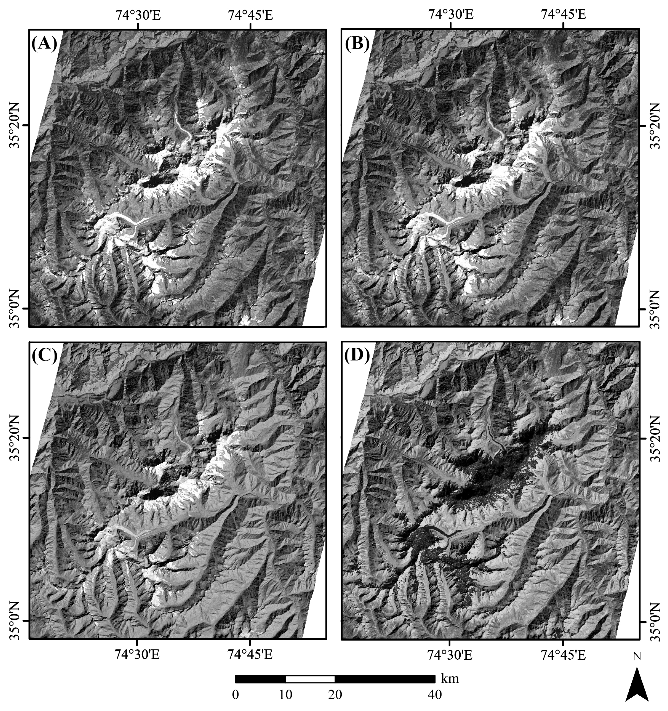
3.3. Simulated ASTER Imagery

All of the aforementioned radiation-transfer parameters were simulated from 0.4 to 3.0 $\mathsf{\mu }$m for each pixel in the scene. We assumed that surface reflectance is Lambertian, and computed the at-satellite radiance ($L^0$) for the full spectrum as:

$$L^0(\lambda )={\rho }_s^c(\lambda )\left[\frac{E_b(\lambda )+E_d(\lambda )}{\pi }\right]T^{\uparrow }(\lambda )+L_p(\lambda ).$$

(17)

We then applied the ASTER spectral-response functions to each $L^0$ spectra and used Equation (16) to simulate the ASTER spectral images. The spectral characteristics of the simulated images are presented in

Table 2. Spectrally Simulated ASTER imagery characteristics. Mean exoatmospheric irradiance at 1 astronomical unit ($E^0$) from Thome et al. [104].

Band	${\mathit{E}}^0[$Wm${}^{-2}\mathsf{\mu }$m${}^{-1}]$	${\mathit{\lambda }}_{\mathit{c}}[\mathsf{\mu }$m]	Spectral Bandwidth $[\mathsf{\mu }$m]
1	1848	0.532	0.484–0.644
2	1549	0.638	0.590–0.731
3	1114	0.760	0.720–0.908
5	225.4	1.658	2.120–2.284

. Although we recognize that surface reflectance characteristics at Nanga Parbat are anisotropic in nature, we did not attempt to simulate the BRDF given a lack of data and our objective to evaluate ARC methods to account for topographic effects in $E_b$, $T^{\downarrow }$, $E_d$, $T^{\uparrow }$, and $L_p$.

It is important to note that we did not simulate the spatial or radiometric resolution of the ASTER sensor, but forced the spatial resolution to coincide with the resolution of the DEM. We also assumed that the sensor could account for the magnitude of the simulated at-satellite radiance values, even though the ASTER sensor exhibits 8-bit radiometric resolution.

3.4. Anisotropic Reflectance Correction

We evaluated a variety of empirical ARC methods. To do so, our evaluation considered an evaluation of whether atmospheric correction is required for suitable topographic correction. Given our RTC simulation, perfect atmospheric correction was applied before topographic correction as follows:

$$L(\lambda )=\frac{L^0(\lambda )-L_p(\lambda )}{T^{\uparrow }(\lambda )}.$$

(18)

The ARC methods we evaluated are as follows, where $L_n$ represents normalized imagery after applying the technique:

• Statistical-Empirical Correction [55,56]. Assuming a linear correlation between at-satellite radiance and local topographic conditions:

  $$L^0(\lambda )={\beta }_0+{\beta }_{1}cosi,$$

  (19a)

  $$L_n(\lambda )=L^0(\lambda )-cosi{\beta }_1-{\beta }_0+{\overline{L}}^0(\lambda ),$$

  (19b)

  where ${\beta }_0$ and ${\beta }_1$ represent the y-intercept and slope coefficient of the linear regression, respectively.
• B-Correction assuming isotropic reflectance conditions [14].

  $$L^0(\lambda )={\beta }_0+{\beta }_{1}cosi,$$

  (20a)

  $$x=L^0(\lambda )-\left({\beta }_0+{\beta }_{1}cosi\right),$$

  (20b)

  $$L_n(\lambda )=L^0(\lambda )+\left({\beta }_1+x\right)\left(cos{\theta }_s-cosi\right),$$

  (20c)

  where ${\beta }_0$ and ${\beta }_1$ represent the y-intercept and slope coefficient of the linear regression, respectively, and x represents the residuals of the radiance data to the predicted regression line.
• B-Correction assuming a non-linear relationship and an anisotropic reflectance model [105].

  $$ln{L}^0(\lambda )={\beta }_0+{\beta }_{1}cosi,$$

  (21a)

  $$L_n(\lambda )=L^0(\lambda )exp\left[{\beta }_1\left(cos{\theta }_s-cosi\right)\right],$$

  (21b)

  where ${\beta }_0$ and ${\beta }_1$ represent the y-intercept and slope coefficient of the linear regression, respectively.
• Variable Empirical Coefficient Algorithm [14].

  $$L^0(\lambda )={\beta }_0+{\beta }_{1}cosi,$$

  (22a)

  $$f_a(\lambda )=\frac{{\overline{L}}^0(\lambda )}{{\beta }_{1}cosi+{\beta }_0},$$

  (22b)

  $$L_n(\lambda )=L^0(\lambda )f_a(\lambda ).$$

  (22c)
• Cosine Correction [55].

  $$L_n(\lambda )=L^0(\lambda )\left[\frac{cos{\theta }_s}{cosi}\right].$$

  (23)
• C-Correction [55].

  $$L^0(\lambda )={\beta }_0+{\beta }_{1}cosi,$$

  (24a)

  $$C={\beta }_0/{\beta }_1,$$

  (24b)

  $$L_n(\lambda )=L^0(\lambda )\left[\frac{cos{\theta }_s+C}{cosi+C}\right].$$

  (24c)
• Sun–Canopy–Sensor Correction [71,72].

  $$L_n(\lambda )=L^0(\lambda )\frac{cos{\theta }_{t}cos{\theta }_s}{cosi}.$$

  (25)
• Sun–Canopy–Sensor + C Correction [72].

  $$L_n(\lambda )=L^0(\lambda )\frac{cos{\theta }_{t}cos{\theta }_s+C}{cosi+C},$$

  (26)

  where C is computed using Equation (24b).
• Global Minnaert Correction [39]:

  $$L_n(\lambda )=\frac{L^0(\lambda )cose}{{cos}^{k}i{cos}^{k}e},$$

  (27)

  where e is the exitance angle ($e={\theta }_t$ for nadir viewing), and k is a globally-derived dimensionless Minnaert coefficient that is wavelength dependent and ranges from 0 to 1. It was calculated using least-squares regression on the variables x and y, where $x=log(cosicose)$ and $y=log(L^{0}cose)$. The slope of the regression equation represents k. The correction procedure defaults to the Lambertian assumption when $k=1.0$.
• Pixel-Based Minnaert Correction [26,76]:

  $$L=L^0\left[\frac{cose}{{(cosecosi)}^k}\right],$$

  (28)

  where k is computed for slope ranges using an interval of five degrees, based on regression analysis using variables x and y.

3.5. Validation and Statistical Analysis

The evaluation of ARC methods is notoriously difficult due to subjective approaches that have been typically used. The magnitude and spatial distribution of $L_n$ resulting from topographically-corrected imagery must be correct to ensure accurate biophysical remote sensing and thematic mapping capabilities. Subjective approaches including visualization, global image statistics and other techniques do not make use of reference data and account for magnitude and correlation structure. Therefore, we compared our simulated surface reflectance values, ${\overline{\rho }}_s$, to computed surface reflectance values (${\rho }_n$) based on the topographically corrected radiance values ($L_n$). Given that we have the exact magnitude of the surface irradiance component simulated, under the Lambertian reflectance assumption:

$${\rho }_n=\frac{\pi L_n(\lambda )}{E_b(\lambda )+E_d(\lambda )}.$$

(29)

Our validation and statistical analysis approach was as follows:

• First, we evaluated the image magnitude of reflectance differences using the Root Mean Squared Error (RMSE) as:

  $$RMSE(\lambda )=\sqrt{\frac{{\sum }_{i=1}^N{\left({\overline{\rho }}_{s,i}(\lambda )-{\rho }_{n,i}(\lambda )\right)}^2}{n}}.$$

  (30)
• We computed the magnitude of the Pearson-Product Moment correlation coefficient (r), to ensure that the spatial variability in reflectance accounts for reflectance variation due to land cover structure and biophysical variation as:

  $$r=\frac{{\sum }_{i=1}^N{\left({\overline{\rho }}_{s,i}-\overline{{\rho }_s}\right)}^2{\left({\rho }_{n,i}-\overline{{\rho }_n}\right)}^2}{\sqrt{{\sum }_{i=1}^N{\left({\overline{\rho }}_{s,i}-\overline{{\rho }_s}\right)}^2}\sqrt{{\sum }_{i=1}^N{\left({\rho }_{n,i}-\overline{{\rho }_n}\right)}^2}}.$$

  (31)
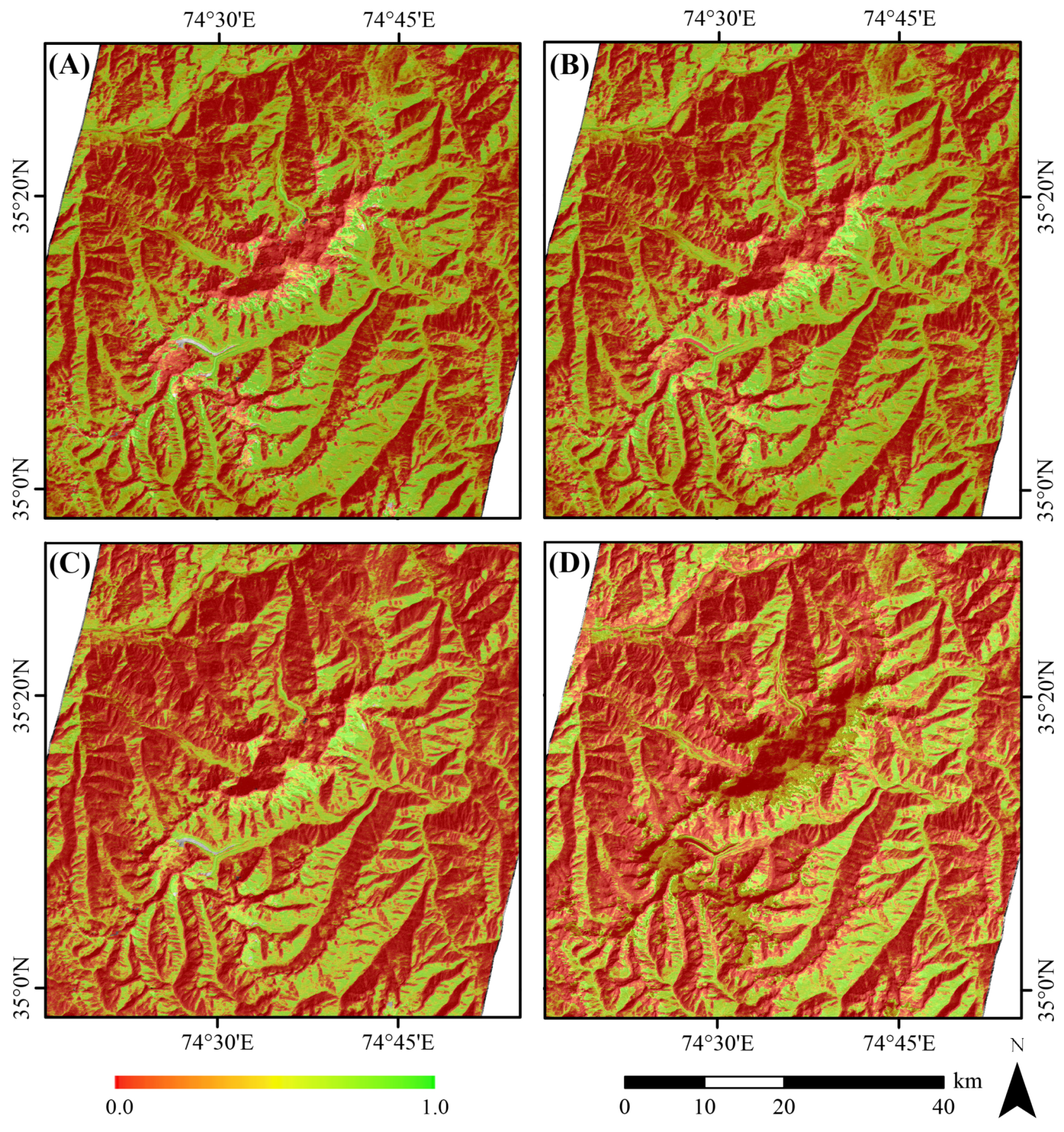
• We then utilized a structural-similarity index (SSI) developed and evaluated by Wang et al. [80] to determine the collective influence of reflectance magnitude (l), global variation (c; contrast) and the correlation coefficient (r), on the topographically corrected reflectance values compared to simulated reflectance. It was computed as follows:

  $${\mu }_{{\rho }_s}=\frac{1}{N}\sum _{i=1}^N{\overline{\rho }}_{s,i},$$

  (32a)

  $${\mu }_{{\rho }_n}=\frac{1}{N}\sum _{i=1}^N{\rho }_{n,i},$$

  (32b)

  $${\sigma }_{{\rho }_s}=\sqrt{\frac{1}{N-1}\sum _{i=1}^N{\left({\overline{\rho }}_{s,i}-{\mu }_{{\rho }_s}\right)}^2},$$

  (32c)

  $${\sigma }_{{\rho }_n}=\sqrt{\frac{1}{N-1}\sum _{i=1}^N{\left({\rho }_{n,i}-{\mu }_{{\rho }_n}\right)}^2},$$

  (32d)

  $$l({\rho }_s,{\rho }_n)=\frac{2{\mu }_{{\rho }_s}{\mu }_{{\rho }_n}+C_1}{{\mu }_{{\rho }_s}^2{\mu }_{{\rho }_n}^2+C_1},$$

  (32e)

  where $C_1={(K_{1}R)}^2$, $K_1$ was set to $0.01$, and R is the dynamic range of an image, which we set to 255, given scaled reflectance images. The contrast was computed as:

  $$c({\rho }_s,{\rho }_n)=\frac{2{\sigma }_{{\rho }_s}{\sigma }_{{\rho }_n}+C_2}{{\sigma }_{{\rho }_s}^2{\sigma }_{{\rho }_n}^2+C_2},$$

  (32f)

  where $C_2={(K_{2}R)}^2$, $K_2$ was set to $0.03$, and R is the dynamic range of an image. Finally, the SSI was computed as:

  $$SSI({\rho }_s,{\rho }_n)={\left[l({\rho }_s,{\rho }_n)\right]}^{2.0}{\left[c({\rho }_s,{\rho }_n)\right]}^{1.0}{\left[r({\rho }_s,{\rho }_n)\right]}^{2.0},$$

  (32g)

  where the SSI index is a coefficient that ranges from 0 to 1, where a 0.0 value indicates no structural similarity, and a value of 1.0 represents identical values, spatial variance and correlation structure. We computed this for each topographic-correction procedure for each spectral band. In this way, we have an integrated metric which accurately evaluates an entire image.
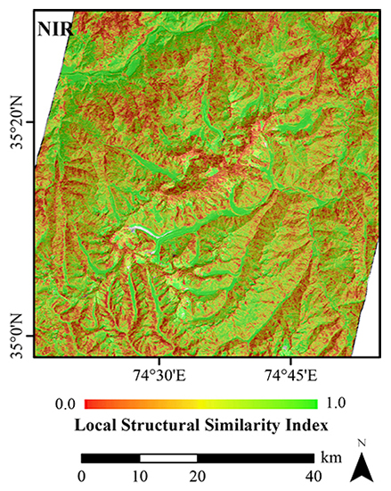
• Nevertheless, to better characterize the spatial nature of how each topographic-correction procedure performs under different topographic conditions, we implemented the SSI over an arbitrary window size of $11\times 11$ to ensure an adequate sample size for computing the statistic. We generated SSI images to evaluate where the topographic-correction procedures worked well, and where they did not. This provided for better interpretation of the results in terms of what topographic conditions cause problems for various techniques.

Perfect topographic correction of imagery should result in a RMSE value of 0.0, the correlation with the surface-reflectance benchmark should be 1.0, and the SSI value should be 1.0 for the globally and locally computed indices. Evaluating the departures from perfect numbers related to application requirements was not our objective, although our evaluation strategy permitted us to determine the degree to which this radiometric calibration issue is addressed over our geographic region.

4. Results

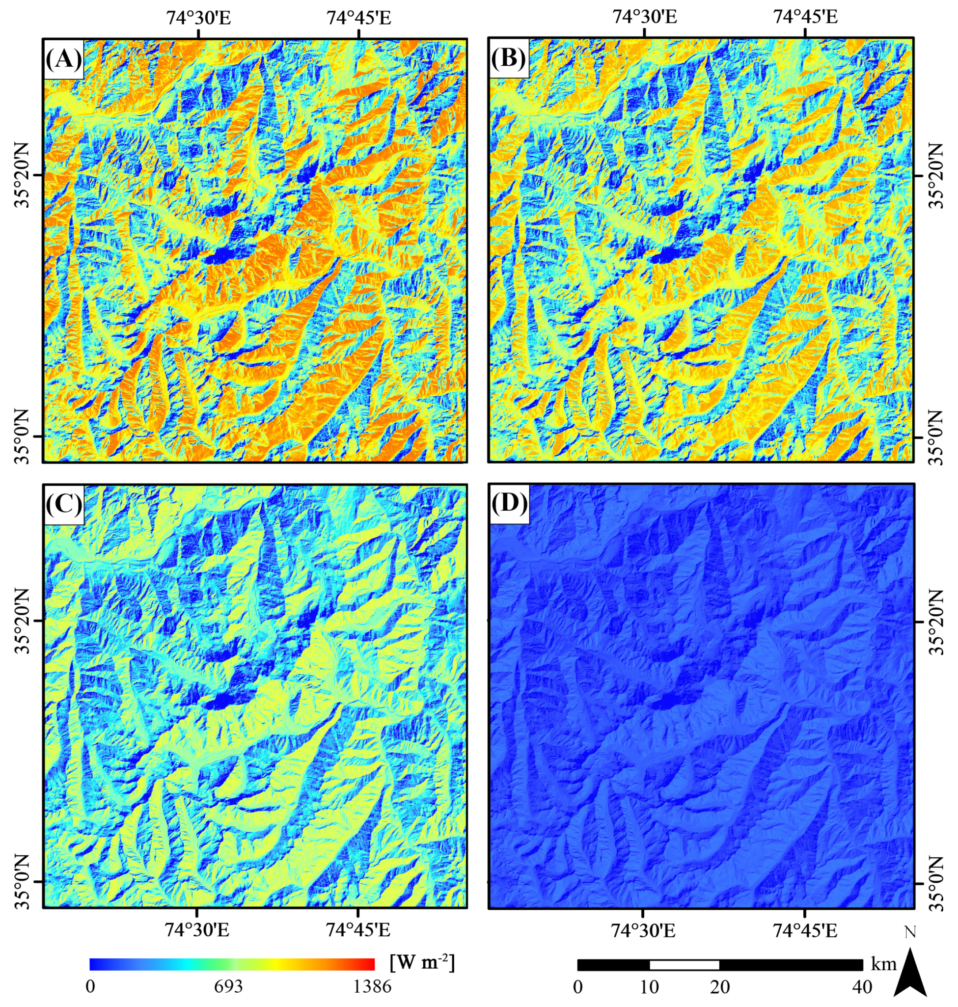
4.1. RTC Simulation

The direct-beam irradiance image is presented in Figure 4. As expected, the magnitude of $E_b$ decreases with longer wavelengths and local topographic effects cause significant spatial variation in irradiance. The northern slopes receive less energy than southern slopes, and cast shadows exist at the highest altitudes on the northern face of Nanga Parbat. Magnitude variations in $E_b$ are larger for shorter wavelength regions, and decreases at longer wavelengths. This can be seen when comparing the green and SWIR bands (Figure 4A,D).

The diffuse-skylight irradiance is presented in Figure 5. In general, the magnitude and spatial variability of $E_d$ decreases with increasing wavelength. This is related to the significant reduction in atmospheric scattering at longer wavelengths. Meso-scale topographic effects can clearly be seen, as the magnitude of $E_d$ is greatest at higher altitudes in glacier accumulation areas, where less topographic shielding occurs. Glacier erosion and river incision generate greater relief that reduces this irradiance component. This can be seen over the Indus River valley in the northwestern portion of the scene.

Figure 6 depicts the atmospheric path-radiance images for ASTER spectral bands. The magnitude of this component is highly wavelength dependent, as greater atmospheric scattering occurs at shorter wavelengths, and lower altitudes increase the optical depth that facilitate greater volumetric atmospheric scattering and higher values of $L_p$. This can be clearly seen in the Indus Valley that exhibits the lowest altitudes in the region (Figure 6A).

The at-satellite radiance images ($L^0$) are presented in Figure 7. Simulated images for the ASTER spectral bands clearly depict the multi-scale topographic effects that are inherent in satellite imagery acquired over this region. The images are extremely realistic and visually similar to real imagery, depicting extreme topographic and land cover spectral variations. Univariate statistics for all the simulated radiation-transfer parameters are presented in

Table 3. Univariate statistical summary of simulated radiation-transfer parameters. These include the downward total transmittance ($T^{\downarrow }$, [unitless]), direct-beam irradiance ($E_b$, $[W$ m${}^{-2}]$), diffuse-skylight irradiance ($E_d$, $[W$ m${}^{-2}]$), surface radiance (L, [W m${}^{-2}$ sr${}^{-1}$$\mathsf{\mu }$m${}^{-1}]$), upward total transmittance ($T^{\uparrow }$, [unitless]), path radiance ($L_p$, [W m${}^{-2}$ sr${}^{-1}$$\mathsf{\mu }$m${}^{-1}]$) and at-satellite radiance ($L^0$, [W m${}^{-2}$ sr${}^{-1}$$\mathsf{\mu }$m${}^{-1}]$).

Metric	${\mathbf{T}}^{\downarrow }$	${\mathbf{E}}_{\mathbf{b}}$	${\mathbf{E}}_{\mathbf{d}}$	L	${\mathbf{T}}^{\uparrow }$	${\mathbf{L}}_{\mathbf{p}}$	${\mathbf{L}}^0$
ASTER Band 1 (Green)
min	0.6440	0.0000	29.5013	3.3221	0.7231	7.9265	15.7990
max	0.6961	1267.8566	167.4728	400.6594	0.7640	20.3858	313.9171
$\mu$	0.6684	732.1280	130.6835	122.2610	0.7418	14.8229	105.3889
$\sigma$	0.0082	344.5620	18.1674	70.1319	0.0065	2.0040	51.8866
ASTER Band 2 (Red)
min	0.7238	0.0000	19.8067	2.2747	0.7872	3.6063	8.2398
max	0.7565	1145.0496	113.7054	351.3746	0.8124	8.7427	288.0417
$\mu$	0.7392	672.3432	88.3678	114.2206	0.7986	6.4451	97.5879
$\sigma$	0.0052	316.2554	12.4042	63.5359	0.0040	0.8287	50.7565
ASTER Band 3 (Near-Infrared, Nadir-Looking)
min	0.7573	0.0000	10.7359	1.7075	0.8081	1.4800	4.3511
max	0.7785	858.5727	62.4444	257.8122	0.8247	3.0548	214.2705
$\mu$	0.7671	507.8256	48.2940	98.6470	0.8153	2.3621	83.2604
$\sigma$	0.0033	238.8220	6.8563	46.0054	0.0026	0.2543	37.7731
ASTER Band 5 (Shortwave Infrared)
min	0.9035	0.0000	0.8501	0.1057	0.9259	0.1739	0.2948
max	0.9085	206.6123	5.0140	109.7754	0.9295	0.2169	102.1068
$\mu$	0.9058	123.6449	3.8577	25.3510	0.9274	0.1942	23.7404
$\sigma$	0.0008	58.1338	0.5542	13.7359	0.0006	0.0086	12.7587

.

4.2. ARC Validation

Validation statistics for characterizing the empirical ARC methods are presented in

Table 4. Statistical summary of anisotropic-reflectance correction methods for spectrally simulated ASTER imagery. Methods include the statistical-empirical correction (SEC), B correction (linear form; BLC), B correction (non-linear form; BNC), variable empirical coefficient algorithm (VECA), Cosine Correction (COSC), C correction (CCOR), sun–canopy–sensor correction (SCS), sun–canopy–sensor plus C correction (SCS+C), global Minnaert Correction (GMC), and pixel-based Minnaert Correction (PMC). Surface radiance related parameters include the minimum surface radiance ($L_{min}$, [W m${}^{-2}$ sr${}^{-1}$$\mathsf{\mu }$m${}^{-1}]$), maximum surface radiance ($L_{max}$, [W m${}^{-2}$ sr${}^{-1}$$\mathsf{\mu }$m${}^{-1}]$), surface radiance (L, [W m${}^{-2}$ sr${}^{-1}$$\mathsf{\mu }$m${}^{-1}]$), and standard deviation of surface radiance ($L_{\sigma }$). Evaluation metrics include the root-mean-squared-error (RMSE), coefficient of determination ($r^2$), and structural-similarity index (ssi).

Method	Band	${\mathit{L}}_{\mathit{m}\mathit{i}\mathit{n}}$	${\mathit{L}}_{\mathit{m}\mathit{a}\mathit{x}}$	$\overline{\mathit{L}}$	${\mathit{L}}_{\mathit{\sigma }}$	RMSE	${\mathit{r}}^2$	ssi	${\mathit{L}}_{\mathit{m}\mathit{i}\mathit{n}}$	${\mathit{L}}_{\mathit{m}\mathit{a}\mathit{x}}$	$\overline{\mathit{L}}$	${\mathit{L}}_{\mathit{\sigma }}$	RMSE	${\mathit{r}}^2$	ssi
		No Atmospheric Correction							Atmospheric Correction
SEC	1	121.4288	419.5435	211.0166	51.8859	0.9166	0.0492	0.0119	125.3453	522.8466	244.2519	70.1432	1.0069	0.0778	0.0155
	2	106.0620	385.8600	195.4078	50.7557	1.1405	0.0374	0.0065	116.4851	465.6465	228.3897	63.5503	1.3131	0.0457	0.0059
	3	87.6831	297.6006	166.5930	37.7716	1.6603	0.0125	0.0008	100.9714	358.5722	198.5007	46.2872	1.9868	0.0134	0.0006
	5	24.2230	126.0190	47.6594	12.7547	5.7374	0.0001	0.0000	25.6837	135.3490	50.9608	13.7520	6.1018	0.0001	0.0000
BLC	1	15.4761	249.9005	109.7295	43.1162	0.2329	0.3141	0.2799	3.5475	317.3839	125.2436	60.6536	0.1461	0.7170	0.6662
	2	7.8863	227.9336	100.4218	42.0368	0.1874	0.4185	0.3865	2.8053	276.5488	116.5728	53.7447	0.1517	0.6774	0.6243
	3	3.7387	167.2680	85.0010	28.3033	0.1732	0.2439	0.1914	1.6250	201.4939	100.9668	35.2306	0.1698	0.3765	0.2975
	5	0.3527	78.6198	23.9415	10.3031	0.1911	0.4517	0.4141	0.0546	84.5305	25.5800	11.1444	0.1739	0.5777	0.5325
BNC	1	17.6215	284.3933	107.5298	47.2864	0.1522	0.4693	0.4624	3.7155	372.1765	123.1868	66.4462	0.0454	0.9547	0.9497
	2	9.1067	264.8636	98.8073	46.9938	0.1082	0.6558	0.6522	2.5919	327.1211	114.9786	59.9968	0.0450	0.9502	0.9456
	3	4.3305	197.0356	84.0492	33.9627	0.0994	0.5129	0.4953	1.6954	240.3360	99.9268	42.2900	0.0534	0.8257	0.8132
	5	0.3356	97.1306	23.8060	12.1413	0.0730	0.8254	0.8248	0.1166	104.8507	25.4470	13.1514	0.0358	0.9651	0.9639
VECA	1	6910.8232	13,5382.1875	45,645.3504	22,377.8885	191.5456	0.6596	0.0000	1267.0876	163,968.6562	50,052.4672	28,726.4287	196.1364	1.0000	0.0000
	2	3432.5625	11,8064.6562	40,186.5106	20,809.4872	184.0312	0.8269	0.0000	948.3248	152,607.8594	49,711.2010	27,618.7049	218.1850	0.9999	0.0000
	3	4499.1143	21,6434.1719	85,997.7968	37,947.9996	510.2392	0.7324	0.0000	1766.3146	26,8510.7812	104,329.7950	47,799.2669	599.3130	0.9922	0.0000
	5	36.6951	11,724.8564	2789.3086	1464.8304	72.3405	0.8896	0.0000	13.5308	13,345.3564	3151.5529	1672.4001	79.8865	0.9930	0.0000
COSC	1	15.0438	2941.4138	162.6748	234.3781	7.1156	0.0152	0.0002	3.3901	2654.2244	166.9583	174.2551	5.0594	0.0339	0.0009
	2	7.6556	1829.7859	136.2113	140.2343	6.2686	0.0174	0.0003	2.6761	1796.4314	149.3772	120.8023	5.1768	0.0291	0.0007
	3	3.6169	947.5345	107.5871	68.1463	5.8571	0.0119	0.0002	1.5613	984.4984	124.3286	63.5167	5.3933	0.0166	0.0002
	5	0.3183	148.2510	27.8217	9.7837	6.6391	0.0030	0.0001	0.1754	144.0357	29.4369	10.2294	5.4759	0.0065	0.0002
		No Atmospheric Correction							Atmospheric Correction
CCOR	1	15.9660	312.7744	105.4528	51.6993	0.1070	0.6596	0.6537	3.0886	399.6947	122.0080	70.0239	0.0013	1.0000	1.0000
	2	8.3396	286.8495	97.6356	50.5584	0.0843	0.8270	0.8115	2.1766	350.2657	114.0964	63.3904	0.0018	0.9999	0.9999
	3	4.3634	209.9650	83.4242	36.8142	0.0883	0.7326	0.7187	1.6812	255.6206	99.3188	45.5049	0.0097	0.9922	0.9920
	5	0.3127	99.9152	23.7681	12.4823	0.0591	0.8896	0.8885	0.1091	107.6200	25.4134	13.4861	0.0156	0.9930	0.9928
SCS	1	7.2744	1968.7629	128.1732	137.7535	4.1202	0.0179	0.0007	1.6482	1784.8512	134.9606	107.4268	2.9371	0.0417	0.0030
	2	3.5878	1226.2263	109.6218	84.0441	3.6292	0.0208	0.0011	1.2167	1206.5087	121.9616	76.5587	3.0044	0.0358	0.0024
	3	1.8233	634.2099	88.1997	41.0922	3.3939	0.0137	0.0005	0.9842	659.8121	102.6753	40.5396	3.1340	0.0193	0.0008
	5	0.1532	99.0919	23.3436	8.4348	3.8411	0.0046	0.0003	0.0896	96.4141	24.7673	9.1094	3.1756	0.0096	0.0007
SCS+C	1	15.9117	312.1077	105.2834	51.6205	0.1069	0.6610	0.6547	3.0768	399.1813	121.8911	69.9566	0.0011	1.0000	1.0000
	2	8.2875	286.0567	97.4600	50.4690	0.0846	0.8283	0.8122	2.1653	349.5909	113.9490	63.3078	0.0015	0.9999	0.9999
	3	4.2623	207.1155	82.6973	36.5041	0.0914	0.7437	0.7272	1.6540	253.1986	98.7162	45.2310	0.0081	0.9929	0.9929
	5	0.2975	98.5728	23.5423	12.3672	0.0598	0.8967	0.8945	0.1043	106.2768	25.1924	13.3716	0.0132	0.9937	0.9937
GMC	1	4.1864	280.1595	89.4138	46.3242	0.1422	0.7086	0.6230	1.0210	356.8810	103.6839	61.6958	0.0988	0.8570	0.8223
	2	2.4318	256.3222	82.9185	44.9469	0.1456	0.8006	0.6971	0.7351	311.4137	97.0110	55.9102	0.1026	0.8360	0.8036
	3	1.2549	189.2264	70.8722	33.6154	0.1693	0.6016	0.5317	0.7256	228.7896	84.4852	41.0439	0.1129	0.5871	0.5686
	5	0.0737	90.1524	20.2470	11.2294	0.1444	0.8166	0.7675	0.0258	96.8096	21.6563	12.0971	0.1240	0.8076	0.7815
PMC	1	13.9944	377.0860	141.4583	49.2648	0.8309	0.0894	0.0284	3.7449	1671.5723	186.4410	81.8467	1.4444	0.1198	0.0163
	2	7.8235	681.3319	144.2308	51.4382	1.3933	0.0640	0.0099	3.0041	1955.2770	182.9376	76.4928	2.1539	0.0744	0.0053
	3	4.4720	848.9163	134.6564	36.3948	2.4773	0.0218	0.0009	1.8724	1847.4973	167.8268	52.2413	3.4374	0.0255	0.0005
	5	0.4382	504.4774	47.1432	22.9189	12.6902	0.0033	0.0000	0.2458	838.8116	52.9906	29.7166	17.2102	0.0045	0.0000

. In general, the so-called statistical-empirical methods did not produce reasonable results. For example, the SEC method produced results with relative high RMSE and low $r^2$ values for all spectral bands. Global SSI values were approximately $0.0$, with or without the use of atmospheric correction. Similarly, for the VECA method, global SSI values were $0.0$ for all spectral bands, with or without the use of atmospheric correction, although RMSE and $r^2$ values were exceptionally high, demonstrating that the scaling factor can account for topographic effects given the Lambertian assumption, although the technique does not produce reasonable values from a magnitude perspective. Our results indicate that the B-Correction method performed the best out of this category of approaches. Specifically, the BNC method outperformed the BLC method with lower RMSE values, and higher $r^2$ and SSI values for all spectral bands. For both methods, improved results were obtained given that imagery were atmospherically corrected before applying topographic correction.

Results for so-called semi-empirical methods assuming Lambertian reflectance are also presented in Table 4. Results were mixed, although several methods generated superior results compared to the other methods evaluated. The COSC and SCS methods performed the most poorly for this category, with relatively high RMSE values, and low $r^2$ and SSI values for all spectral bands. Atmospheric correction before topographic correction did not significantly affect the results for these methods. Conversely, the CCOR and SCS+C methods performed the best given atmospherically corrected imagery, with relatively low RMSE values and high $r^2$ and SSI values for all spectral bands. Both techniques remove almost all the multi-scale topographic variation, and the corrected imagery represents the inherent spectral variation related to land cover structure and biophysical variation. It is important to note, however, that atmospheric correction makes a significant difference and accounts for approximately 10–35% of the explained variability due to topographic coupling that governs atmospheric conditions, depending on the spectral band.

The results for so-called semi-empirical methods assuming non-Lambertian reflectance are also presented in Table 4. The GMC method outperformed the PMC method, and atmospheric correction improved topographic correction results for the GMC method. It did not, however, outperform the BNC, CCOR and SCS+C methods. These results are not surprising given that we utilized the Lambertian assumption in our simulations, and that a proxy parameter for $E_d$ is not included in the GMC and PMC parameterization schemes.

Statistics characterizing the local SSI index for each method (given atmospheric correction) evaluated are presented in

Table 5. Univariate statistics for structural-similarity index (SSI) images based on comparison of simulated reflectance and normalized reflectance given atmospheric correction. Statistics parameters include the minimum (Min), maximum (Max), mean ($\mu$), and standard deviation ($\sigma$) of local $SSI$ values in the image.

Method	Band	Min	Max	$\mathit{\mu }$	$\mathit{\sigma }$
SEC	1	0.0000	0.9264	0.2977	0.2856
	2	0.0000	0.9173	0.2894	0.2854
	3	0.0000	0.8858	0.2160	0.2662
	5	0.0000	0.8521	0.2167	0.2667
BLC	1	0.0000	0.9997	0.6382	0.2745
	2	0.0000	0.9997	0.6168	0.2807
	3	0.0000	0.9988	0.4007	0.2844
	5	0.0000	0.9999	0.4838	0.3343
BNC	1	0.0000	1.0000	0.8924	0.2027
	2	0.0000	1.0000	0.8967	0.1803
	3	0.0000	0.9999	0.7842	0.2231
	5	0.0000	1.0000	0.8522	0.2396
VECA	1	0.0000	0.0000	0.0000	0.0000
	2	0.0000	0.0000	0.0000	0.0000
	3	0.0000	0.0000	0.0000	0.0000
	5	0.0000	0.0001	0.0000	0.0000
COSC	1	0.0000	0.9996	0.3829	0.3571
	2	0.0000	0.9996	0.3681	0.3534
	3	0.0000	0.9971	0.2347	0.2969
	5	0.0000	0.9996	0.2803	0.3384
CCOR	1	0.0000	1.0000	0.9987	0.0131
	2	0.0000	1.0000	0.9969	0.0501
	3	0.0000	1.0000	0.9856	0.0274
	5	0.0000	1.0000	0.9409	0.1408
SCS	1	0.0000	0.9996	0.3672	0.3163
	2	0.0000	0.9997	0.3501	0.3130
	3	0.0000	0.9965	0.1969	0.2428
	5	0.0000	0.9997	0.2536	0.2989
SCS+C	1	0.0001	1.0000	0.9989	0.0122
	2	0.0000	1.0000	0.9970	0.0500
	3	0.0000	1.0000	0.9878	0.0248
	5	0.0000	1.0000	0.9468	0.1303
GMC	1	0.0000	1.0000	0.7425	0.2576
	2	0.0000	1.0000	0.7264	0.2636
	3	0.0000	1.0000	0.5297	0.2947
	5	0.0000	1.0000	0.5783	0.3327
PMC	1	0.0000	0.9999	0.3593	0.3609
	2	0.0000	0.9999	0.3240	0.3539
	3	0.0000	0.9997	0.1925	0.2802
	5	0.0000	0.9977	0.1734	0.2821

. The minimum and maximum values of the local SSI index reveal that all methods produced good and bad correction results, suggesting that these methods produce highly variable results over a large geographic region depending upon the spatial variability in morphometric properties. Perhaps the best metric to evaluate is the mean local SSI value that provides an overall assessment of local topographic-correction effectiveness. In this regard, it is clear that the CCOR and the SCS+C methods produce the most superior results, with the SCS+C method technically outperforming the CCOR. Examination of SSI images indicate that both methods effectively correct for multi-scale topographic effects in simulated imagery. It is interesting to note that these methods do not perform as well on the SWIR spectral band, compared to the other bands, as numerous locations exhibit local SSI values <0.5. These locations are associated with relatively high-altitude ridge tops and steep slopes near ridges throughout the scene. This suggests that the methods do not adequately account for the diffuse-skylight irradiance at longer wavelengths, given the use of a proxy parameter that better represents diffuse irradiance at shorter wavelengths given more atmospheric scattering.

Most other methods exhibit relatively low local SSI values throughout the scene. Topographic correction results are highly variable, and in general, topographic correction is superior on sunlit slopes. For example, the SEC method that has been noted for being superior for topographic correction cannot account for multi-scale topographic effects. Figure 8 clearly depicts very low local SSI values on north, northwestern facing slopes (red), whereas sunlit slopes exhibit higher SSI values (green). Methods that produce higher mean SSI values, such as the BNC and the GMC methods produce results that appear to be wavelength and spatially dependent. For example, the BNC method (Figure 9) works better for the green and red regions of the spectrum, but the diffuse-irradiance component cannot be accounted for at high altitude on steep slopes. The results for the NIR and SWIR bands are more spatially variable than results in shorter wavelengths and the method does not effectively account for less variation in the diffuse irradiance in these regions of the spectrum. Similarly, Figure 10 depicts high variability in SSI values for all spectral bands from correction using the GMC method, although the spatial variability in accuracy is higher in the NIR and SWIR bands.

5. Discussion

Radiation-transfer simulations and our theoretical assessment of empirical ARC methods reveal new insights into the nature of research involving the evaluation of topographic-correction methods. Our results clearly reveal that the methods we evaluated did not reasonably account for multi-scale topographic effects, countering results presented in the literature. The magnitude of reflectance and the correlation structure of biophysical properties were not preserved in the topographically-corrected imagery. Our best results are obtained by using the CCOR and SCS+C methods, although comprehensive atmospheric correction is required.

We are surprised that the CCOR and SCS+C methods accounted for multi-scale topographic effects related to the diffuse-skylight irradiance component. The C parameter is an empirical coefficient that is thought to be able to account for the variation in $E_d$. Although the authors who introduced the CCOR were not definitive in their description of the C parameter [55,72], it has since become commonly accepted in the literature that C accounts for $E_d$, e.g., [16,26,57]. This is not possible, however, because it is a wavelength dependent constant that does not covary with $E_d$. It is used to modify ${\theta }_s$ and $cosi$, such that the ratio-scaling factor is highly correlated to $E_b+E_d$, thereby accounting for the primary topographic effects in our simulation. This suggests that ${\theta }_s$ accounts for some variation in $E_d$ related to diffuse scattering, and that $cosi$ also accounts for variation in topographic shielding given steep slopes, as $E_b$ is relatively low with steeper slopes. Nevertheless, we should expect both of these methods to be totally inadequate for removing multi-scale topographic effects in real imagery, given that a multitude of other topographic factors govern $E_t$, the BRDF, and therefore other secondary radiation-transfer parameters, as all of the methods evaluated cannot account for these more complex radiation-transfer parameters due to their limited parameterization schemes.

Our results strongly suggest that these empirical methods cannot be used to address the problem of multi-scale topographic effects, given the simplicity of their parameterization schemes. Other multi-scale topographic effects must be accounted for [8], as well as the anisotropic nature of atmospheric scattering on $E_d$ and the BRDF [8,106]. The literature assumes that there is a best correction method for different environments and that investigators should evaluate a variety of methods on a case-by-case basis and use the best one, e.g., [18]. This assumption is most likely false given that high spatial variability in topographic and land cover conditions governs the magnitude and spatial variation in wavelength dependent radiation-transfer parameters, as our simulation demonstrates. Furthermore, this assumption is based on the belief that researchers can accurately evaluate topographic-correction procedures, accounting for magnitudes and the spectral correlation structure of land cover and biophysical variations, which is effectively a radiometric calibration issue. This information over an entire geographic region is generally not available in mountain environments. Therefore, common evaluation procedures are inadequate. Recently, investigators have begun to recognize this fact and have utilized a multi-criteria-based approach where numerous evaluation methods are considered, e.g., [63]. We note, however, that these approaches cannot account for variations in numerous radiation-transfer parameters that are governed by topographic effects.

Fundamentally, the inherent nature-of-the-problem stems from inadequate parameterization schemes and inadequate evaluation approaches. ARC is fundamentally a radiometric calibration issue that requires the removal of spectral variation caused by coupled atmosphere–topography effects. Evaluation procedures must account for various radiation-transfer parameters in order to remove those image information components. The use of previously reported evaluation procedures are highly subjective given unrealistic assumptions. The issues include:

• The use of the human visualization system to evaluate empirical ARC methods. Decreased spectral variation is thought to signify effective topographic correction. This approach cannot be used to evaluate the degree of information compression given the use of a scaling factor, the correct magnitude of surface reflectance, or the spatial variation structure of surface spectral reflectance. Furthermore, interpretation is subject to biases resulting from a-priori experience, generalization caused by 8-bit display monitors, color bins, and graphic production techniques.
• The concept of similar surface reflectance conditions for homogeneous landcover is assumed to be the result of effective ARC. This assumption is not realistic in mountain environments because of biophysical property variation related to topography and land cover structure. Environmental dynamics in mountain environments determine the magnitude and extent of various processes which dramatically alter surface irradiance, surface composition and the BRDF. These include processes such as evapotranspiration, gravitational sediment fluxes, erosion, deposition and slope stability that governs plant dispersion and mineralogical composition. In addition, climate forcing and variations in temperature and precipitation govern vegetation density, glaciation and snow cover. ARC methods need to work over large spatial and temporal scales, therefore the operational scale dependencies of processes may vary significantly, and the assumption that homogeneous land cover conditions will exhibit similar reflectance on illuminated and shadowed terrain, which serves as a basis for evaluation, does not account for spatial variation in surface-process dynamics and radiation-transfer theory.
• The relationship between $cosi$ and L should not be used to evaluate the effectiveness of topographic correction, as it does not account for numerous radiation-transfer parameters (e.g., $E_d$ and $E_t$) that exhibit spectral variation at different scales and magnitudes than $cosi$. In addition, land cover patterns are dependent upon topographic variables and residual correlations between $cosi$, and spectral reflectance values would be expected following topographic corrections [18,63]. Furthermore, as we have demonstrated, a global image evaluation procedure cannot be used to account for local effectiveness of a topographic-correction method.
• It is frequently assumed that spectral homogeneity should increase after topographic correction, e.g., [18]. This assumption is not consistent with the concept of enhancing the moderate- to high-frequency surface reflectance conditions, as lower-frequency topographic information is reduced. This was demonstrated by Bishop and Colby [15], who used semi-variogram analysis to evaluate surface reflectance variability after topographic correction. This is especially the case in more dynamic mountain environments where moisture variations, sediment fluxes, and anthropogenic forcing can cause significant compositional and biophysical variation that can increase spectral variation over various spatial scales.
• The utilization of classification accuracy as a way to evaluate topographic correction. This approach is extremely problematic and does not address numerous radiometric calibration issues related to the fundamental radiation-transfer components. The magnitude and spatial variation of reflectance is also not accounted for. It introduces significant uncertainty given various assumptions, and is influenced by overcorrection or information compression, the nature of the algorithm, training, as well as dimensionality of the feature space and specific information components making up that feature space. Therefore, many potential sources of error are intrinsic in the classification process [19,50]. Given high spectral variability in mountain environments, and the availability of high resolution imagery, good classification accuracy can be difficult to obtain given increased spectral variation. Nevertheless, good classification results do not equate to optimized ARC results that need to be representative of surface biophysical property variation to enable the prediction of surface parameters and generation of thematic information.
• Issues of empiricism associated with using parameter values and thresholds to modify results for a particular geographic region. Often, such attempts are applied over relatively small geographic areas, and their utilization may become questionable over larger regions due to more spatial variability in morphometric properties of the topography and RT parameters. We would argue that, given the paucity of data over large areas by which to formally validate ARC results, investigators cannot effectively select the appropriate magnitude or interval range of parameters in an attempt to optimize results. For example, empirically modifying results based on visual interpretation does not effectively address the removal of radiation-transfer components from the imagery, as the parameterization schemes and modification procedures cannot deterministically account for other topographic effects. It also results in non-repeatable results, as such procedures may not produce consistent results in different environments, at different times, or with different analysts. Consequently, empiricism is also partially responsible for inconsistent results presented in the literature.
• Research involving the ranking of empirical ARC procedures. We would argue that this should not be a research objective, as traditional statistical and classification evaluation methods do not account for the reduction of radiation-transfer components encapsulated in multispectral imagery. As demonstrated in our simulation, radiometric calibration is required and the results are highly dependent upon the wavelength region, time, and morphometric properties of the topography. Most of these factors have not been systematically evaluated. Rather, investigators assume that more evaluation procedures are better and produce reliable results when, in fact, the radiometric calibration issues are not being addressed using simplistic empirical ARC procedures. Rankings which are based on different evaluation approaches also lead to inconsistencies in the literature.
• Mountain topographic and spectral variability. The literature is ubiquitous with statements indicating that investigators are evaluating ARC methods in complex topography. Complexity needs to be semantically defined, as indicated by Bishop and Dobreva [107], who evaluated the term from morphometric property and system perspectives. Clearly, the magnitude and spatial variability of morphometric properties govern the multi-scale topographic effects that partially regulate irradiance and reflectance variations. As demonstrated, even secondary or tertiary parameters can significantly influence results if they are not formally accounted for (i.e., need for atmospheric correction given relief variations). Similarly, the radiation-transfer process dynamics need to be accounted for in order to represent their variation adequately so that it can be removed. Consequently, we could expect that various empirical ARC methods will better function in environments with less topographic and spectral variability. We would argue that the concept needs to be evaluated from a radiation-transfer systems perspective. Therefore, researchers need to account for the morphometric properties of the topography within their study areas.
• Small angle approximation. Most investigators utilize constant solar geometry parameters for atmospheric correction, the cosine of the incidence angle and ARC methods. Solar geometry parameters vary for each pixel and are a function of time, latitude, longitude, and altitude. The computation of these parameters is more important for processing large regions or scenes compared to small areas. Nevertheless, it is assumed that the variance is insignificant. It is yet unclear as to the impact that this assumption has on ARC, as it is a parameter that partially governs atmospheric transmittance, path radiance, direct irradiance, diffuse-skylight irradiance, adjacent-terrain irradiance and the BRDF.
• Performance dependence on land cover. Numerous researchers have indicated that the effectiveness of empirical ARC methods is largely dependent on land-surface types, e.g., [17,81,108]. We would argue that this is not technically correct, as effective ARC depends upon a multitude of factors including: (1) parameterization scheme of technique/model; (2) spatial variability in morphometric properties; (3) landcover type and structure; and (4) sensor characteristics, such as wavelength. Clearly, the morphometric properties of the topography coupled with atmospheric conditions and the land cover surface structure will collectively govern the irradiance fluxes and the BRDF. Sensor-system characteristics will then determine the level of generalization associated with recording the RTC. Empirical ARC methods do not formally account for all of the radiation-transfer components that are caused by multi-scale topographic effects, especially the BRDF. It has yet to be conclusively determined to what degree the BRDF accounts for spectral variation in imagery. In such dynamic environments, areal and intimate mixtures of matter must also be accounted for, and is another factor governing the BRDF.

Our simulation results strongly suggest that inconsistencies in research results can be understood on the basis of environmental complexity, as it governs radiation-transfer parameters. Less complex topography, and more spatially homogeneous land cover conditions, may dictate that a reduced number of radiation-transfer parameters need to be accounted for, and that $E_b$ may be the most dominant factor. Under these conditions, various empirical ARC methods may work to some degree. As the environmental complexity increases, however, different approaches may need to be used. Nevertheless, ARC investigations do not generally account for a multitude of multi-scale topographic effects and parameters related to atmospheric conditions, cast shadows, $E_d$, $E_t$, or the BRDF. Although empirical methods that assume non-Lambertian reflectance have been evaluated, the parameters that govern the BRDF are not fully accounted for. Furthermore, parameterization scheme errors have propagated in the literature, and researchers may have utilized different or incorrect equations for some ARC methods. To complicate matters, researchers have demonstrated that results are temporally variable, e.g., [54].

The aforementioned issues demonstrate the multi-faceted complexity of ARC. Numerous radiation-transfer components are collectively governed by atmospheric conditions, multi-scale topographic effects and landcover dynamics. Characterizing and removing these variance components from multispectral imagery is notoriously difficult and will require radiation-transfer modeling. We should not expect the use of a few proxy parameters to address the nature-of-the-problem given the anisotropic nature of irradiance and reflectance. Furthermore, more research is warranted on developing and evaluating new parameterization schemes that better account for variations in the components of the RTC. More research investigating topographic effects on the BRDF is sorely needed. Only in this way will we be able to better understand which radiation-transfer components must be accounted for in ARC methods and models.

6. Conclusions

Remote sensing of mountain environments is challenging, as multi-scale topographic effects govern the anisotropic nature of the radiation-transfer cascade. Although anisotropic-reflectance correction investigations have been ongoing for approximately 40 years, inconsistent research results caused by inadequate evaluation approaches have resulted in little progress on effective topographic correction of multispectral imagery in mountain environments. Consequently, we diagnostically evaluated commonly used empirical ARC methods using spectrally simulated ASTER imagery over the Nanga Parbat, Himalaya. Specifically, we used first-order radiation-transfer modeling to account for a variety of spectral, spatial and temporal factors including orbital dynamics, atmospheric absorption and scattering, direct- and diffuse-skylight irradiance, land cover structure, and surface biophysical variations.

As expected, we found that the dominance and spatial variability of various radiation-transfer components were wavelength dependent. Our results clearly reveal that most of the empirical ARC methods we evaluated could not effectively or reasonably account for the multi-scale topographic effects at Nanga Parbat. The magnitude of reflectance and the correlation structure of biophysical properties were not preserved in the topographically-corrected multispectral imagery. Using a Lambertian assumption, better results were obtained using the CCOR and SCS+C methods, although comprehensive atmospheric correction was required, and we did not account for other primary and secondary topographic effects that are thought to significantly influence spectral variation in imagery acquired over mountains (adjacent-terrain irradiance and the BRDF). Evaluation of structural-similarity images revealed spatially variable results that are wavelength dependent. Collectively, our simulation and evaluation procedures strongly suggest that empirical ARC methods cannot be used to address the problem of multi-scale topographic effects in mountain environments, given the simplicity of the parameterization schemes and their inability to adequately account for anisotropic irradiance and reflectance.

Characterizing and removing radiation-transfer parameter variance components from multispectral imagery is notoriously difficult and will require radiation-transfer modeling efforts. More research is warranted on developing and evaluating new parameterization schemes that better account for variations in the components of the RTC. More research investigating topographic effects on the BRDF is sorely needed. The next phase of our research will be to incorporate more primary, secondary and tertiary parameters of the RTC to evaluate ARC methods.

References

- Zhang, Y.; Li, X.; Wen, J.; Liu, Q.; Yan, G. Improved Topographic Normalization for Landsat TM Images by Introducing the MODIS Surface BRDF. Remote Sens. 2015, 7, 6558–6575. [Google Scholar] [CrossRef]
- Schaepman, M.E.; Ustin, S.L.; Plaza, A.J.; Painter, T.H.; Verrelst, J.; Liang, S. Earth system science related imaging spectroscopy-An assessment. Remote Sens. Environ. 2009, 113, S123–S137. [Google Scholar] [CrossRef]
- Bishop, M.P.; Shroder, J.F., Jr.; Bonk, R.; Olsenholler, J. Geomorphic Change in High Mountains: A Western Himalayan Perspective. Glob. Planet. Chang. 2002, 32, 311–329. [Google Scholar] [CrossRef]
- Bishop, M.P.; Bush, A.B.G.; Copland, L.; Kamp, U.; Owen, L.A.; Seong, Y.B.; Shroder, J.F., Jr. Climate Change and Mountain Topographic Evolution in the Central Karakoram, Pakistan. Ann. Assoc. Am. Geogr. 2010, 100, 772–793. [Google Scholar] [CrossRef]
- Bishop, M.P.; James, L.A.; Shroder, J.F., Jr.; Walsh, S.J. Geospatial Technologies and Digital Geomorphological Mapping: Concepts, Issues and Research. Geomorphology 2012, 137, 5–26. [Google Scholar] [CrossRef]
- Kargel, J.S.; Leonard, G.J.; Shugar, D.H.; Haritashya, U.K.; Bevington, A.; Fielding, E.J.; Fujita, K.; Geertsema, M.; Miles, E.S.; Steiner, J.; et al. Geomorphic and geologic controls of geohazards induced by Nepal’s 2015 Gorkha earthquake. Science 2016, 351. [Google Scholar] [CrossRef] [PubMed]
- Weiss, D.J.; Walsh, S.J. Remote Sensing of Mountain Environments. Geogr. Compass 2009, 3, 1–21. [Google Scholar] [CrossRef]
- Proy, C.; Tanré, D.; Deschamps, P.Y. Evaluation of topographic effects in remotely sensed data. Remote Sens. Environ. 1989, 30, 21–32. [Google Scholar] [CrossRef]
- Justice, C.; Holben, B.N. Examination of Larnbertian and Non-Lambertian Models for Simulating the Topographic Effect on Remotely Sensed Data; Technical Report; NASA: Washington, DC, USA, 1979.
- Justice, C.O.; Wharton, S.W.; Holben, B.N. Application of Digital Terrain Data to Quantify and Reduce the Topographic Effect on Landsat Data; Technical Report; National Aeronautics and Space Administration: Washington, DC, USA, 1980.
- Colby, J.D. Topographic normalization in rugged terrain. Photogramm. Eng. Remote Sens. 1991, 57, 531–537. [Google Scholar]
- Gupta, S.K.; Shukla, D.P. Evaluation of topographic correction methods for LULC preparation based on multi-source DEMs and Landsat-8 imagery. Spat. Inf. Res. 2019. [Google Scholar] [CrossRef]
- Hurni, K.; Hoek, J.V.D.; Fox, J. Assessing the spatial, spectral, and temporal consistency of topographically corrected Landsat time series composites across the mountainous forests of Nepal. Remote Sens. Environ. 2019, 231, 111225. [Google Scholar] [CrossRef]
- Gao, Y.; Zhang, W. A simple empirical topographic correction method for ETM+ imagery. Int. J. Remote Sens. 2009, 30, 2259–2275. [Google Scholar] [CrossRef]
- Bishop, M.P.; Colby, J.D. Topographic normalization of multispectral satellite imagery. In Encyclopedia of Snow, Ice and Glaciers; Springer: Dordrecht, The Netherlands, 2011; pp. 1187–1196. [Google Scholar] [CrossRef]
- Richter, R.; Kellenberger, T.; Kaufmann, H. Comparison of Topographic Correction Methods. Remote Sens. 2009, 1, 184–196. [Google Scholar] [CrossRef]
- Goslee, S.C. Topographic corrections of satellite data for regional monitoring. Photogramm. Eng. Remote Sens. 2012, 78, 973–981. [Google Scholar] [CrossRef]
- Wu, Q.; Jin, Y.; Fan, H. Evaluating and comparing performances of topographic correction methods based on multi-source DEMs and Landsat-8 OLI data. Int. J. Remote Sens. 2016, 37, 4712–4730. [Google Scholar] [CrossRef]
- Bishop, M.P.; Colby, J.D. Anisotropic reflectance correction of SPOT-3 HRV imagery. Int. J. Remote Sens. 2002, 23, 2125–2131. [Google Scholar] [CrossRef]
- Bishop, M.P.; Shroder, J.F., Jr. Remote Sensing and Geomorphometric Assessment of Topographic Complexity and Erosion Dynamics in the Nanga Parbat Massif. In Tectonics of the Nanga Parbat Syntaxis and the Western Himalaya; The Geological Society of London: London, UK, 2000; pp. 181–199. [Google Scholar]
- Berger, A. Long-Term Variations of Daily Insolation and Quaternary Climatic Changes. J. Atmos. Sci. 1978, 35, 2362–2367. [Google Scholar] [CrossRef]
- Jacobson, M.Z. Fundamentals of Atmospheric Modeling, 2nd ed.; Cambridge University Press: Cambridge, UK, 2005. [Google Scholar]
- Chavez, J. Image-based atmospheric correction—Revisted and improved. Photogramm. Eng. Remote Sens. 1996, 62, 1025–1036. [Google Scholar]
- Gueymard, C. SMARTS2, a Simple Model of the Atmospheric Radiative Transfer of Sunshine: Algorithms and Performance Assessment; Florida Solar Energy Center: Cocoa, FL, USA, 1995. [Google Scholar]
- Bird, R.E.; Riordan, C. Simple Solar Spectral Model for Direct and Diffuse Irradiance on Horizontal and Tilted Planes at the Earth’s Surface for Cloudless Atmospheres. J. Clim. Appl. Meteorol. 1986, 25, 87–97. [Google Scholar] [CrossRef]
- Vanonckelen, S.; Lhermitte, S.; Rompaey, A.V. The effect of atmospheric and topographic correction methods on land cover classification accuracy. Int. J. Appl. Earth Obs. Geoinf. 2013, 24, 9–21. [Google Scholar] [CrossRef]
- Dozier, J.; Bruno, J.; Downey, P. A faster solution to the horizon problem. Comput. Geosci. 1981, 7, 145–151. [Google Scholar] [CrossRef]
- Rossi, R.E.; Dungan, J.L.; Beck, L.R. Kriging in the shadows: Geostatistical interpolation for remote sensing. Remote Sens. Environ. 1994, 49, 32–40. [Google Scholar] [CrossRef]
- Dubayah, R.; Rich, P.M. Topographic solar radiation models for GIS. Int. J. Geogr. Inf. Syst. 1995, 9, 405–419. [Google Scholar] [CrossRef]
- Giles, P.T. Remote sensing and cast shadows in mountainous terrain. Photogramm. Eng. Remote Sens. 2001, 67, 833–839. [Google Scholar]
- Perez, R.; Stewart, R.; Arbogast, C.; Seals, R.; Scott, J. An anisotropic hourly diffuse radiation model for sloping surfaces: Description, performance validation, site dependency evaluation. Sol. Energy 1986, 36, 481–497. [Google Scholar] [CrossRef]
- Wilson, J.P.; Bishop, M.P. Geomorphometry. In Remote Sensing and GIScience in Geomorphology; Bishop, M.P., Shroder, J.F., Eds.; Academic Press: Waltham, MA, USA, 2013; pp. 162–186. [Google Scholar]
- Kondratyev, K.Y.; Fedorova, M.P. Radiation Regime of Inclined Surfaces; Technical Report; World Meteorological Organization: Geneva, Switzerland, 1977. [Google Scholar]
- Temps, R.C.; Coulson, K.L. Solar radiation incident upon slopes of different orientations. Sol. Energy 1977, 19, 179–184. [Google Scholar] [CrossRef]
- Kimes, D.S.; Kirchner, J.A. Modeling the effects of various radiant transfers in mountainous terrain on sensor response. IEEE Trans. Geosci. Remote Sens. 1981, GE-19, 100–108. [Google Scholar] [CrossRef]
- Roberts, G. A review of the application of BRDF models to infer land cover parameters at regional and global scales. Prog. Phys. Geogr. 2001, 25, 483–511. [Google Scholar] [CrossRef]
- Li, F.; Jupp, D.L.B.; Thankappan, M.; Lymburner, L.; Mueller, N.; Lewis, A.; Held, A. A physics-based atmospheric and BRDF correction for Landsat data over mountainous terrain. Remote Sens. Environ. 2012, 124, 756–770. [Google Scholar] [CrossRef]
- Brook, A.; Polinova, M.; Ben-Dor, E. Fine tuning of the SVC method for airborne hyperspectral sensors: The BRDF correction of the calibration nets targets. Remote Sens. Environ. 2018, 204, 861–871. [Google Scholar] [CrossRef]
- Smith, J.A.; Lin, T.L.; Ranson, K.J. The Lambertian Assumption and LANDSAT Data. Photogramm. Eng. Remote Sens. 1980, 46, 1183–1189. [Google Scholar]
- Hugli, H.; Frei, W. Understanding anisotropic reflectance in mountainous terrain. Photogramm. Eng. Remote Sens. 1983, 49, 671–683. [Google Scholar]
- Hall, D.K.; Chang, A.T.C. Reflectance of glaciers as calculated using Landsat-5 Thematic Mapper data. Remote Sens. Environ. 1988, 25, 311–321. [Google Scholar] [CrossRef]
- Dozier, J. Spectral signature of alpine snow cover from the Landsat Thematic Mapper. Remote Sens. Environ. 1989, 28, 9–22. [Google Scholar] [CrossRef]
- Aniya, M.; Sato, H.; Naruse, R.; Skvarca, P.; Casassa, G. The use of satellite and airborne imagery to inventory outlet glaciers of the southern Patagonia Icefield, South America. Photogramm. Eng. Remote Sens. 1996, 62, 1361–1369. [Google Scholar]
- Greuell, W.; de Ruyter de Wildt, M. Anisotropic reflection by melting glacier ice: Measurements and parametrizations in Landsat TM bands 2 and 4. Remote Sens. Environ. 1999, 70, 265–277. [Google Scholar] [CrossRef]
- Bishop, M.P.; Colby, J.D.; Luvall, J.C.; Quattrochi, D.; Rickman, D.L. Remote-sensing science and technology for studying mountain environments. In Geographic Information Science and Mountain Geomorphology; Bishop, M.P., Shroder, J.F., Jr., Eds.; Springer: Chichester, UK, 2004; pp. 147–187. [Google Scholar]
- Iqbal, M. An Introduction to Solar Radiation; Academic Press: Toronto, ON, Canada, 1983. [Google Scholar]
- Liang, S. Quantitative Remote Sensing of Land Surfaces; Wiley: Hoboken, NJ, USA, 2004. [Google Scholar]
- Hoffer, R.M. Natural Resource Mapping in Mountainous Terrain by Computer Analysis of ERTS-1 Satellite Data; Purdue University Laboratory for Applications of Remote Sensing, LARS Research Bulletin 919; Purdue University: West Lafayette, Indiana, 1975; 124p. [Google Scholar]
- Riaño, D.; Chuvieco, E.; Salas, J.; Aguado, I. Assessment of different topographic corrections in Landsat-TM data for mapping vegetation types. IEEE Trans. Geosci. Remote Sens. 2003, 41, 1056–1061. [Google Scholar] [CrossRef] [Green Version]
- Ghasemi, N.; Mohammadzadeh, A.; Sahebi, M.R. Assessment of different topographic correction methods in ALOS AVNIR-2 data over a forest area. Int. J. Digit. Earth 2013, 6, 504–520. [Google Scholar] [CrossRef]
- Li, H.; Xu, L.; Shen, H.; Zhang, L. A general variational framework considering cast shadows for the topographic correction of remote sensing imagery. ISPRS J. Photogramm. Remote Sens. 2016, 117, 161–171. [Google Scholar] [CrossRef]
- Holben, B.N.; Justice, C.O. The topographic effects on spectral response fromnadir-point sensors. Photogramm. Eng. Remote Sens. 1980, 46, 1191–1200. [Google Scholar]
- Franklin, S.E. Image transformations in mountainous terrain and the relationship to surface patterns. Comput. Geosci. 1991, 17, 1137–1149. [Google Scholar] [CrossRef]
- Zhang, Z.; Wulf, R.R.D.; Coillie, F.M.B.V.; Verbeke, L.P.C.; Clercq, E.M.D.; Ou, X. Influence of different topographic correction strategies on mountain vegetation classification accuracy in the Lancang Watershed, China. J. Appl. Remote Sens. 2011, 5, 1–21. [Google Scholar] [CrossRef]
- Teillet, P.M.; Guindon, B.; Goodenough, D.G. On the Slope-Aspect Correction of Multispectral Scanner Data. Can. J. Remote Sens. 1982, 8, 84–106. [Google Scholar] [CrossRef] [Green Version]
- Meyer, P.; Itten, K.I.; Kellenberger, T.; Sandmeier, S.; Sandmeier, R. Radiometric corrections of topographically induced effects on Landsat TM data in an alpine environment. ISPRS J. Photogramm. Remote Sens. 1993, 48, 17–28. [Google Scholar] [CrossRef]
- Fan, W.; Li, J.; Liu, Q.; Zhang, Q.; Yin, G.; Li, A.; Zeng, Y.; Xu, B.; Xu, X.; Zhou, G.; et al. Topographic Correction of Forest Image Data Based on the Canopy Reflectance Model for Sloping Terrains in Multiple Forward Mode. Remote Sens. 2018, 10, 717. [Google Scholar] [CrossRef] [Green Version]
- McDonald, E.R.; Wu, X.; Caccetta, P.A.; Campbell, N.A. Illumination correction of Landsat TM data in South East NSW. In Proceedings of the Tenth Australasian Remote Sensing and Photogrammetry Conference, Adelaide, Australia, 21–25 August 2000. [Google Scholar]
- Soenen, S.A.; Peddle, D.R.; Coburn, C.A.; Hall, R.J.; Hall, F.G. Improved topographic correction of forest image data using a 3-D canopy reflectance model in multiple forward mode. Int. J. Remote Sens. 2008, 29, 1007–1027. [Google Scholar] [CrossRef]
- Wu, J.; Bauer, M.E.; Wang, D.; Manson, S.M. A comparison of illumination geometry-based methods for topographic correction of QuickBird images of an undulant area. ISPRS J. Photogramm. Remote Sens. 2008, 63, 223–236. [Google Scholar] [CrossRef]
- Hantson, S.; Chuvieco, E. Evaluation of different topographic correction methods for Landsat imagery. Int. J. Appl. Earth Obs. Geoinf. 2011, 13, 691–700. [Google Scholar] [CrossRef]
- Pimple, U.; Sitthi, A.; Simonetti, D.; Pungkul, S.; Leadprathom, K.; Chidthaisong, A. Topographic Correction of Landsat TM-5 and Landsat OLI-8 Imagery to Improve the Performance of Forest Classification in the Mountainous Terrain of Northeast Thailand. Sustainability 2017, 9, 258. [Google Scholar] [CrossRef] [Green Version]
- Sola, I.; González-Audícana, M.; Álvarez-Mozos, J. Multi-criteria evaluation of topographic correction methods. Remote Sens. Environ. 2016, 184, 247–262. [Google Scholar] [CrossRef] [Green Version]
- Vincini, M.; Reeder, D.; Frazzi, E. An empirical topographic normalization method for forest TM data. IEEE Int. Geosci. Remote Sens. Symp. 2002, 4, 2091–2093. [Google Scholar]
- Justice, C.O.; Wharton, S.W.; Holben, B.N. Application of digital terrain data to quantify and reduce the topographic effect on Landsat data. Int. J. Remote Sens. 1981, 2, 213–230. [Google Scholar] [CrossRef] [Green Version]
- Civco, D.L. Topographic normalization of Landsat Thematic Mapper digital imagery. Photogramm. Eng. Remote Sens. 1989, 55, 1303–1309. [Google Scholar]
- Ekstrand, S. Landsat TM-based forest damage assessment: Correction for topographic effects. Photogramm. Eng. Remote Sens. 1996, 62, 151–161. [Google Scholar]
- Karathanassi, V.; Andronis, V.; Rokos, D. Evaluation of the topographic normalization methods for a Mediterranean forest area. Int. Achives Photogramm. Remote Sens. 2000, 33, 654–661. [Google Scholar]
- Ediriweera, S.; Pathirana, S.; Danaher, T.; Nichols, D.; Moffiet, T. Evaluation of Different Topographic Corrections for Landsat TM Data by Prediction of Foliage Projective Cover (FPC) in Topographically Complex Landscapes. Remote Sens. 2013, 5, 6767–6789. [Google Scholar] [CrossRef] [Green Version]
- Mishra, V.D.; Sharma, J.K.; Khanna, R. Review of topographic analysis methods for the western Himalaya using AWiFS and MODIS satellite imagery. Ann. Glaciol. 2010, 51, 153–160. [Google Scholar] [CrossRef] [Green Version]
- Gu, D.; Gillespie, A. Topographic Normalization of Landsat TM Images of Forest Based on Subpixel Sun–Canopy–Sensor Geometry. Remote Sens. Environ. 1998, 64, 166–175. [Google Scholar] [CrossRef]
- Soenen, S.A.; Peddle, D.R.; Coburn, C.A. SCS+C: A modified Sun-canopy-sensor topographic correction in forested terrain. IEEE Trans. Geosci. Remote Sens. 2005, 43, 2148–2159. [Google Scholar] [CrossRef]
- Moreira, E.P.; Valeriano, M.M. Application and evaluation of topographic correction methods to improve land cover mapping using object-based classification. Int. J. Appl. Earth Obs. Geoinf. 2014, 32, 208–217. [Google Scholar] [CrossRef]
- Minnaert, J.L. The reciprocity principle in lunar photometry. Astrophys. J. 1941, 93, 403–410. [Google Scholar] [CrossRef]
- Colby, J.D.; Keating, P.L. Land cover classification using Landsat TM imagery in the tropical highlands: The influence of anisotropic reflectance. Int. J. Remote Sens. 1998, 19, 1479–1500. [Google Scholar] [CrossRef]
- Lu, D.; Ge, H.; He, S.; Xu, A.; Zhou, G.; Du, H. Pixel-based Minnaert Correction Method for Reducing Topographic Effects on a Landsat 7 ETM+ Image. Photogramm. Eng. Remote Sens. 2008, 74, 1343–1350. [Google Scholar] [CrossRef] [Green Version]
- Conese, C.; Gilabert, M.A.; Maselli, F.; Bottai, L. Topographic normalization of TM scenes through the use of an atmospheric correction method and digital terrain models. Photogramm. Eng. Remote Sens. 1993, 59, 1745–1753. [Google Scholar]
- Gitas, I.Z.; Devereux, B.J. The role of topographic correction in mapping recently burned Mediterranean forest areas from LANDSAT TM images. Int. J. Remote Sens. 2006, 27, 41–54. [Google Scholar] [CrossRef]
- Sola, I.; González-Audícana, M.; Álvarez-Mozos, J.; Torres, J.L. Synthetic images for evaluating topographic correction algorithms. IEEE Trans. Geosci. Remote Sens. 2014, 52, 1799–1810. [Google Scholar] [CrossRef]
- Wang, Z.; Bovik, A.C.; Sheikh, H.R.; Simoncelli, E.P. Image quality assessment: From error measurement to structural similarity. IEEE Trans. Image Process. 2004, 13, 600–612. [Google Scholar] [CrossRef] [Green Version]
- Park, S.; Jung, H.; Choi, J.; Jeon, S. A quantitative method to evaluate the performance of topographic correction models used to improve land cover identification. Adv. Space Res. 2017, 60, 1488–1503. [Google Scholar] [CrossRef]
- Shroder, J.F., Jr.; Bishop, M.P. Unroofing of the Nanga Parbat Himalaya. In Tectonics of the Nanga Parbat Syntaxis and the Western Himalaya; The Geological Society of London: London, UK, 2000; pp. 163–179. [Google Scholar]
- Zeitler, P.K.; Koons, P.O.; Bishop, M.P.; Chamberlain, C.P.; Craw, D.; Edwards, M.A.; Hamidullah, S.; Jan, M.Q.; Khan, M.A.; Khattak, M.U.K.; et al. Crustal Reworking at Nanga Parbat, Pakistan: Metamorphic Consequences of Thermal-Mechanical Coupling Facilitated by Erosion. Tectonics 2001, 20, 712–728. [Google Scholar] [CrossRef]
- NASA/METI/AIST/Japan Spacesystems; U.S./Japan ASTER Science Team. ASTER GDEM, Version 2; Data Set; NASA: Washington, DC, USA, 2009. [CrossRef]
- Kokaly, R.F.; Clark, R.N.; Swayze, G.A.; Livo, K.E.; Hoefen, T.M.; Pearson, N.C.; Wise, R.A.; Benzel, W.M.; Lowers, H.A.; Driscoll, R.L.; et al. USGS Spectral Library Version 7; Technical Report; U.S. Geological Survey: Reston, VA, USA, 2017. [CrossRef]
- Baldridge, A.M.; Hook, S.J.; Grove, C.I.; Rivera, G. The ASTER spectral library version 2.0. Remote Sens. Environ. 2009, 113, 711–715. [Google Scholar] [CrossRef]
- U.S. Naval Observatory; Nautical Alamanc Office. The Astronomical Almanac; U.S. Naval Observatory; Nautical Almanac Office: Washington, DC, USA, 2013. [Google Scholar]
- NOAA; U.S. Air Force. U.S. Standard Atmosphere; Technical Report; NOAA: Silver Spring, MA, USA, 1976.
- Leckner, B. The spectral distribution of solar radiation at the Earth’s surface—Elements of a model. Sol. Energy 1978, 20, 143–150. [Google Scholar] [CrossRef]
- Kasten, F. A new table and approximation formula for the relative optical air mass. Archiv für Meteorol. Geophys. Bioklimatol. Ser. B 1965, 14, 206–223. [Google Scholar] [CrossRef]
- Dozier, J. A clear-sky spectral solar radiation model for snow-covered mountainous terrain. Water Resour. Res. 1980, 16, 709–718. [Google Scholar] [CrossRef] [Green Version]
- Kääb, A.; Wessels, R.; Haeberli, W.; Huggle, C.; Kargel, J.S.; Jodha, S.; Khalsa, S. Rapid ASTER imaging facilitates timely assessment of glacier hazards and disasters. EOS 2003, 84, 117–124. [Google Scholar] [CrossRef]
- Gjermundsen, E.F.; Mathieu, R.; Kääb, A.; Chinn, T.; Fitzharris, B.; Hagen, J.O. Assessment of multispectral glacier mapping methods and derivation of glacier area changes, 1978–2002, in the central Southern Alps, New Zealand, from ASTER satellite data, field survey and existing inventory data. J. Glaciol. 2011, 57, 667–683. [Google Scholar] [CrossRef] [Green Version]
- Shukla, A.; Gupta, R.P.; Arora, M.K. Delineation of debris-covered glacier boundaries using optical and thermal remote sensing data. Remote Sens. Lett. 2010, 1, 11–17. [Google Scholar] [CrossRef]
- Yüksel, A.; Akay, A.E.; Gundogan, R. Using ASTER imagery in land use/cover classification of eastern Mediterranean landscapes according to CORINE land cover project. Sensors 2008, 8, 1237–1251. [Google Scholar] [CrossRef] [Green Version]
- Hu, X.; Weng, Q. Estimating impervious surfaces from medium spatial resolution imagery: A comparison between fuzzy classification and LSMA. Int. J. Remote Sens. 2011, 32, 5645–5663. [Google Scholar] [CrossRef]
- Butler, R.W.H.; George, M.; Harris, N.B.W.; Jones, C.; Prior, D.J.; Treloar, P.J.; Wheeler, J. Geology of the northern part of the Nanga Parbat massif, northern Pakistan, and its implications for Himalayan tectonics. J. Geol. Soc. 1992, 149, 557–567. [Google Scholar] [CrossRef]
- Garzanti, E.; Vezzoli, G.; Andò, S.; Paparella, P.; Clift, P.D. Petrology of Indus River sands: A key to interpret erosion history of the Western Himalayan Syntaxis. Earth Planet. Sci. Lett. 2005, 229, 287–302. [Google Scholar] [CrossRef]
- Vance, D.; Bickle, M.; Ivy-Ochs, S.; Kubik, P.W. Erosion and exhumation in the Himalaya from cosmogenic isotope inventories of river sediments. Earth Planet. Sci. Lett. 2003, 206, 273–288. [Google Scholar] [CrossRef]
- Sarmast, M.; Farpoor, M.H.; Boroujeni, I.E. Soil and desert varnish developments as indicators of landform evolution in central Iranian deserts. Catena 2017, 149, 98–109. [Google Scholar] [CrossRef]
- Potter, R.M.; Rossman, G.R. The manganese- and iron-oxide mineralogy of desert varnish. Chem. Geol. 1979, 25, 79–94. [Google Scholar] [CrossRef]
- Hapke, B. Bidirection reflectance spectroscopy. 1. Theory. J. Geophys. Res. 1981, 86, 3039–3054. [Google Scholar] [CrossRef]
- Wiscombe, W.J. Improved Mie scattering algorithms. Appl. Opt. 1980, 19, 1505–1509. [Google Scholar] [CrossRef] [PubMed]
- Thome, K.J.; Biggar, S.F.; Slater, P.N. Effects of assumed solar spectral irradiance on intercomparisons of earth-observing sensors. In Proceedings of SPIE; Fujisada, H., Lurie, J.B., Weber, K., Eds.; International Society for Optics and Photonics: Bellingham, WA, USA, 2001; Volume 4540, pp. 260–269. [Google Scholar] [CrossRef]
- Vincini, M.; Frazzi, E. Multitemporal evaluation of topographic normalization methods on deciduous forest TM data. IEEE Trans. Geosci. Remote Sens. 2003, 41, 2586–2590. [Google Scholar] [CrossRef]
- Perez, R.; Seals, R.; Ineichen, P.; Steward, R.; Menicucci, D. A new simplified version of the perez diffuse irradiance model for tilted surfaces. Sol. Energy 1987, 39, 221–231. [Google Scholar] [CrossRef] [Green Version]
- Bishop, M.P.; Dobreva, I.D. Geomorphometry and Mountain Geodynamics: Issues of Scale and Complexity. In Integrating Scale in Remote Sensing and GIS; Quattrochi, D.A., Wentz, E., Lam, N.S.N., Emerson, C.W., Eds.; Taylor and Francis: Boca Raton, FL, USA, 2017; Chapter 7; pp. 189–228. [Google Scholar] [CrossRef]
- Singh, M.; Mishra, V.D.; Thakur, N.K. Expansion of empirical-statistical based topographic correction algorithm for reflectance modeling on Himalayan terrain using AWiFS and MODIS sensor. J. Indian Soc. Remote Sens. 2015, 43, 379–393. [Google Scholar] [CrossRef]