An Efficient Compressive Hyperspectral Imaging Algorithm Based on Sequential Computations of Alternating Least Squares

Division of Global Business and Technology, Hankuk University of Foreign Studies, Yongin 17035, Korea
Remote Sens. 2019, 11(24), 2932; https://doi.org/10.3390/rs11242932
Submission received: 23 October 2019
/
Revised: 28 November 2019
/
Accepted: 3 December 2019
/
Published: 6 December 2019
Abstract
:Hyperspectral imaging is widely used to many applications as it includes both spatial and spectral distributions of a target scene. However, a compression, or a low multilinear rank approximation of hyperspectral imaging data, is required owing to the difficult manipulation of the massive amount of data. In this paper, we propose an efficient algorithm for higher order singular value decomposition that enables the decomposition of a tensor into a compressed tensor multiplied by orthogonal factor matrices. Specifically, we sequentially compute low rank factor matrices from the Tucker-1 model optimization problems via an alternating least squares approach. Experiments with real world hyperspectral imaging revealed that the proposed algorithm could compute the compressed tensor with a higher computational speed, but with no significant difference in accuracy of compression compared to the other tensor decomposition-based compression algorithms.

1. Introduction
Hyperspectral imaging (HSI) allows one to provide information on the spatial and spectral distributions of a target scene simultaneously by acquiring up to hundreds of narrow and adjacent spectral band images ranging from ultraviolet to far-infrared electromagnetic spectrum [1,2]. To do this, an imaging sensor such as a charged coupled device collects the different wavelengths dispersed from the incoming light. Then, the signals captured by the imaging sensor are digitized and arranged into pixels of a two-dimensional image , where I denotes the size of X-directional spatial information, and is the number of quantized spectra of the signals. The procedure of capturing the pixels as an X-directional single line continues until the spatial range reaches J, which is the Y-directional size of the entire target scene. Finally, HSI constructs a three-dimensional data . Once the HSI data are obtained, they can be used in many applications, such as detecting and identifying objects at a distance in environmental monitoring [3] or medical image processing [4], finding anomaly in automatic visual inspection [5], or detecting and identifying targets of interest [6,7]. However, as the area of the target scene or the number of quantized spectra increase, the manipulation of demands prohibitively large computational resources and storage space. To overcome this, efficient compression techniques must be employed as preprocessing for applications to filter out some redundancy along their adjacent spectral bands or spatial information, thereby reducing the size of .
Owing to the shape of HSI data, the typical mathematical basis for compression techniques is based on tensor decompositions, because it facilitates the simultaneous preservation and analysis of the spatial and spectral structures of data [8]. Fang et al. used canonical polyadic decomposition (CPD) for dimension reduction of HSI data, where CPD decomposes a tensor into several rank-one tensors [9,10]. De Lathauwer et al. suggested a Tucker decomposition-based low rank approximation algorithm of a tensor, where Tucker decomposition decomposes a tensor into a smaller sized core tensor multiplied by a factor matrix along each mode [11]. In this study, we considered Tucker decomposition for compressing HSI data. Specifically, we focused on developing an efficient algorithm to compute a higher order singular value decomposition (HOSVD), which is a special case of Tucker decomposition with orthogonal constraints on the factor matrices. Subsequently, we applied it to compression problems from real world HSI data.
The remainder of this paper is organized as follows. Section 2 defines the notations and preliminaries frequently used in this paper. Section 3 briefly explains the well-known algorithms for computing HOSVD for a compression. Section 4 introduces the algorithm we propose. Section 5 provides the experimental results, and Section 6 concludes the paper.
2. Notations and Preliminaries
Here, we define the symbols and terminology for the simplicity of notation and presentation. We use calligraphic letters to denote tensors, e.g., ; boldface capital letters for matrices, e.g., ; boldface lowercase letters for vectors, e.g., ; and lowercase letters for scalars, e.g., a. We define an operation of tensor-matrix multiplication between an arbitrary N-th order tensor and a matrix along mode-n, such that
where and the -th element of is computed by
for arbitrary and . Note that the values and are the elements of and , respectively [12].
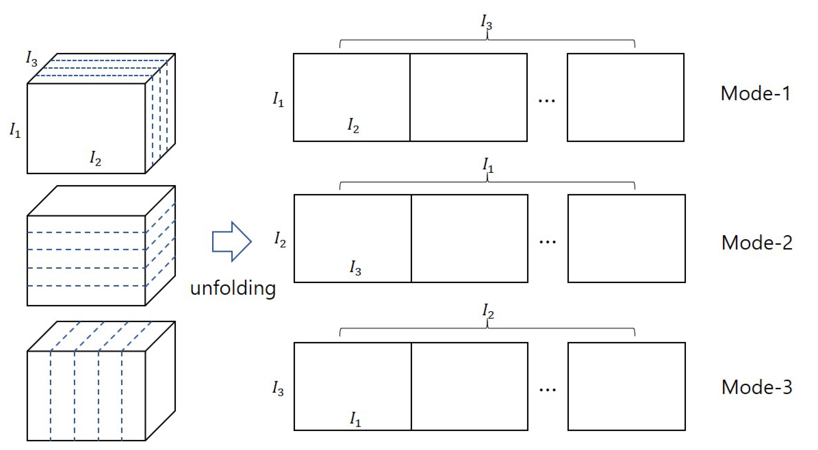
A tensor can be matricized with mode-n, after rearranging each element of appropriately. For example, a third order tensor is matricized along each mode, as shown in Figure 1.
The Frobenius norm of a tensor is the square root of the sum of the squares of all elements in , such that
3. Related Works
We briefly revisit here, well-known algorithms to compute HOSVD of a tensor. HOSVD, which is a special case of Tucker decomposition that has an orthogonal constraint, decomposes an N-th order tensor into factor matrices and a core tensor such that
while satisfying a constraint , where a matrix represents an identity matrix [11]. Here, a factor matrix is considered as the principal components in each mode, and elements of a core tensor reveal the level of interactions between the different components. Note that , and we denote as multilinear ranks of . The representation of with the form of (1) is not unique. Thus, there are many algorithms to compute (1). One of the simplest methods to obtain and is computing leading singular vectors of each unfolding matrix of such that
where indicates the mode-n unfolding matrix of . Then a core tensor is obtained from , and is regarded as a compressed tensor of . Despite its simple procedure of computation, a single step of applying singular value decomposition (SVD) is insufficient to improve approximations of in many contexts. De Lathauwer et al. proposed a more accurate algorithm of computing HOSVD via iterative computations of SVD, called higher order orthogonal iterations (HOOI) [13]. HOOI is designed to solve the optimization problem of finding and , such that
Since , the minimization problem (3) is identical to finding ; thus, by definition,
Therefore, HOOI obtains each factor matrix independently from the , leading singular vectors of the unfolding matrix matricized from along mode-k while fixing the other factor matrices. The iterations continue until the output converges. The procedure of HOOI is summarized in Algorithm 1 for . In practice, HOOI produces more accurate outputs than those from the algorithm based on (2); it is considered one of the most accurate algorithms for obtaining HOSVD from a tensor. Therefore, many hyperspectral compression techniques have been developed based on HOOI. For example, Zhang et. al applied HOOI to the compression of HSI [14]. An et al. suggested the method based on [11] with an adaptive, multilinear rank estimation, and applied it to HSI compression [15]. However, iterative computations of SVD require huge computational resources. Additionally, the number of iterations for convergence is difficult to predict.
To overcome these limitations, Elden et al. proposed a Newton–Grassman based algorithm that guaranteed quadratic convergence and fewer iteration steps than HOOI [16]. However a single iteration of the algorithm is much more expensive owing to the computation of the Hessian. Sorber et al. introduced a quasi-Newton optimization algorithm that iteratively improves the initial guess by using a quasi-Newton method from the nonlinear cost function [17]. Hassanzadeh and karami proposed a block coordinate descent search based algorithm [18], which updates the factor matrices initialized by using compressed sensing. Instead of employing SVD for unfolding matrices, Phan et al. proposed a fast algorithm based on a Crank–Nicholson-like technique, which has a lower computational cost in a single step compared with HOOI [19]. Lee proposed a HOSVD algorithm based on an alternating least squares method that recycles the intermediate results of computations for one factor matrix to the other computations [20]. In contrast to the algorithm proposed by [20], which computes the Tucker-1 model optimization individually along each mode, the proposed algorithm considers sub-problems of computing a factor matrix simultaneously in a single iteration. This approach enables more accurate computation of the intermediate results in each iteration.
| Algorithm 1 |
| Input: |
| Output: |
| 1: for l = 1, 2, 3, … do |
| 2: for n = 1, 2, 3 do |
| 3: |
| 4: |
| 5: = leading singular vectors of |
| 6: end for |
| 7: |
| 8: if then |
| 9: break |
| 10: end if |
| 11: end for |
4. Sequential Computations of Alternating Least Squares for Efficient HOSVD
In the proposed algorithm, we sequentially compute low multilinear rank factor matrices from the Tucker-1 model optimization problems via an alternating least squares approach. For simplicity, and to consider the shape of a HSI data, we only used a third order tensor in this study. However, the extension of the algorithm for application to any dimensional tensors without loss of generality is straightforward.
Assume that we have a third order tensor . Our goal is to decompose to
where represents an orthogonal factor matrix along mode-n, is the appropriate truncation level or n-multilinear rank, and denotes the core tensor. Then, we rewrite the formulation of the optimization problem of finding and in (3) as
Before starting the explanation, we note that the order of computation for each factor matrix does not need to be fixed. However, for convenience we will present the procedure for solving our optimization problems from the order of (1,2,3) mode. Let . Then, the problem of finding in (6) is equivalent to the problem of finding the solution from the Tucker-1 model optimization of , such that
where denotes an identity matrix. Here, we can see that the tensor is a Tucker-2 model, but it can be used to formulate another Tucker-1 optimization problem of finding , such that
where . Similarly, to find , we use the optimization problem of Tucker-1 model, which is given by
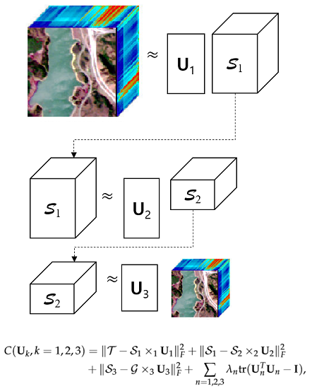
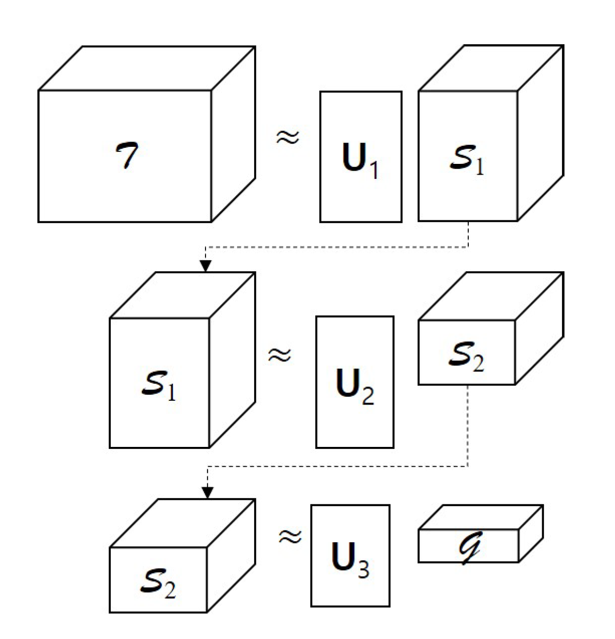
We illustrate the sequential procedure for the Tucker-1 model optimization problems in Figure 2. Let us consider the optimization problems (7)–(9) simultaneously. Then, the optimal factor matrices of the tensor are computed by solving the minimization problem of the cost function , which is defined as
where the parameters represent the Lagrangian multipliers, and the function computes the trace of an arbitrary matrix . Because the cost function in (10) has too many unknown variables, an alternating least squares method that optimizes one variable while leaving the others fixed, is a proper approach. First, by taking a derivative of with respect to while regarding the other variables as constant values, and matricizing those along mode-1, we obtain
where is the unfolding matrix of along mode-1. Thus, from (11), we can compute as follows:
After is obtained, the next step is to compute while fixing and the others to recycle the intermediate results for computing the others. After updating in (12) and by taking a derivative to (10) with respect to , we can compute such that
Because the orthogonal constraint must be satisfied, we reorthogonalize by simply applying QR-decomposition.
Next, we find . After updating and , we take a derivative of with respect to and rearrange the terms similar to the procedure of computing . Then, we obtain
where and are the unfolding matrices of and along mode-2, respectively. Then, we can compute with fixed such that
Finally, is obtained by solving
where and are the unfolding matrices from the tensor and along mode-3, respectively.
Algorithm 2 summarizes the procedure explained in this section. Note that the function in steps 6, 10, and 14, returns the unfolding matrix from an arbitrary tensor along mode-i, and the function in steps 9, 13, and 16 returns the reorthogonalized matrix from by applying QR decomposition. If we assume that the size of an input tensor is , and its initial multilinear rank is , then the most expensive step in Algorithm 2 occurs at the computation of in step 7, and its computational complexity is approximately operations, which is similar to those of the other HOSVD algorithms. Additionally, unlike HOOI, we eliminate independence from the computation of each factor matrix by reusing intermediate tensors and factor matrices to find a specific factor matrix. Thus, we expected the proposed algorithm to achieve better convergence to the solution.
| Algorithm 2 |
| Input: |
| Output: |
| 1: for l = 1, 2, 3, … do |
| 2: for n = 1 to 3 do |
| 3: Rearrange the order such that |
| 4: |
| 5: |
| 6: , and |
| 7: |
| 8: |
| 9: |
| 10: , and |
| 11: |
| 12: |
| 13: |
| 14: , and |
| 15: |
| 16: |
| 17: |
| 18: if then |
| 19: break |
| 20: end if |
| 21: end for |
| 22: end for |
5. Experiments
We begin this section by introducing the experimental settings. Then, we compare the performance of Algorithm 2 to those of the other well-known HOSVD algorithms by showing an application to real-world HSI data.
5.1. Experimental Settings
Our experiments were performed on Intel i9 processor with 32 GB of memory. We developed the software for the experiments using MATLAB version 9.6.0.1135713. For the real-world HSI dataset, we used three datasets which are widely used for testing classification or compression performance of HSI data. Details on these datasets are as follows.
- –
- Jasper Ridge: Jasper Ridge dataset was captured by an airborne visible/infrared imaging spectrometer (AVIRIS) sensor by the Jet Propulsion Laboratory. The spatial size of the dataset is with 224 channels, in which its quantized spectra range is from 380 nm to 2500 nm. There are four endmembers in this dataset, which include “road,” “soil,” “water,” and “tree.” Detailed information regarding Jasper Ridge dataset is provided in [21].
- –
- Indian Pines: Indian pine dataset was captured by AVIRIS sensor over the Indian pine test site in North-western Indiana. The scenery is comprised of agriculture, forest or natural perennial vegetation. The spatial size of the dataset used in the experiments was with 224 channels ranging from 400 nm to 2500 nm. Detailed information of Indian Pines dataset is provided in [22].
- –
- Urban: Urban dataset was recorded by a hyperspectral digital image collection experiment (HYDICE) sensor; its location is an urban area at Copperas Cove in Texas. The spatial size of the dataset is with 221 channels, in which its quantized spectral range is from 400 nm to 2500 nm. There are four endmembers to be classified; namely, “asphalt,” “grass,” “tree,” and “roof.” More information about Urban dataset is provided in [21].
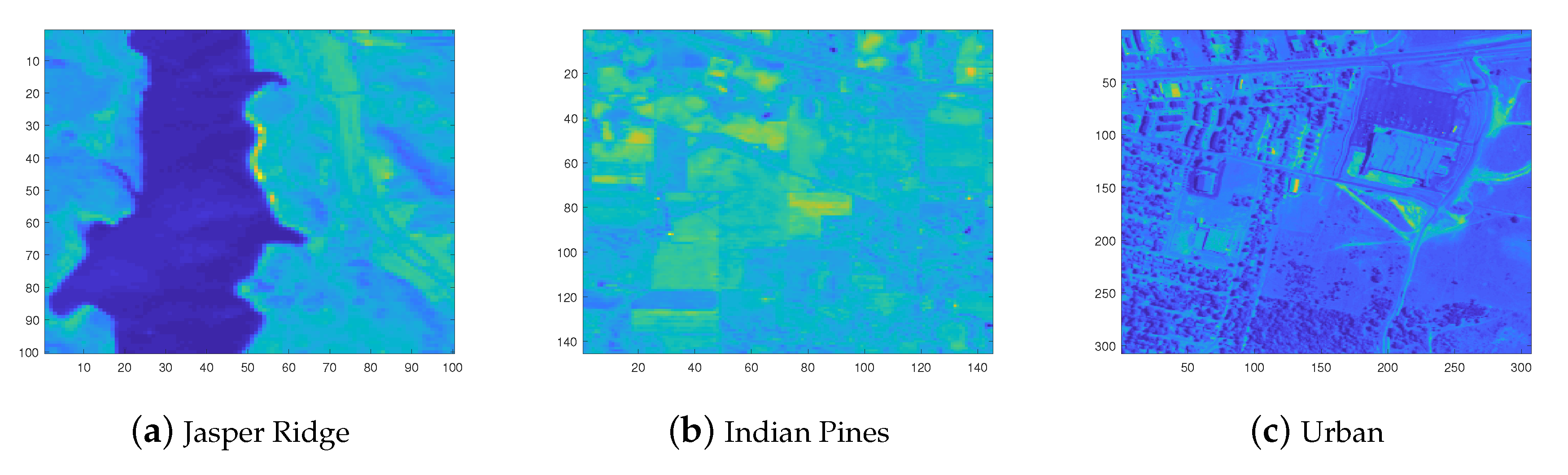
Figure 3 depicts the average intensities of pixels throughout the spectrum. The datasets are represented as tensors; for example, the Jasper Ridge dataset is denoted by .
To compare the performances of the proposed algorithm with previous algorithms, we evaluated the relative errors and the execution times with the algorithm from HOOI, a Crank–Nicholson-like algorithm for HOSVD (CrNc henceforce) [19]; a quasi-Newton-based nonlinear least squares algorithm (henceforce HOSVD_NLS) [17]; and a method based on block coordinate descent search [18] which is a slight modification of the algorithm described in [23] (henceforth BCD-CD). Here, the relative errors, denoted as relerr, are defined such that
where and are the tensors before and after applying compression algorithms, respectively. The programs implementing HOOI and HOSVD_NLS algorithms, are from [24]. Note that the stopping criterion of all the algorithms in the comparison is equal, and it is defined as
where indicates a user-defined threshold. The maximum iteration number is 100. To measure the execution time of each algorithm, we repeat the experiments 10 times and take the average from the results.
The initial factor matrices with low multilinear ranks of all algorithms are computed from SVD-based HOSVD algorithm described in (2) (henceforth, HOSVD) when the truncation level in mode-, satisfies the condition
where represents the i-th largest singular value of the mode-n unfolding matrix from , and is the user-defined threshold to adjust the compression rate of the spectral and spatial dimensions of . Specifically, we set the value to 0.05, 0.1, 0.2, and 0.3. Table 1 lists the low multilinear ranks in each case after applying HOSVD. Note that the sizes of the core tensors from all algorithms are identical.
5.2. Experimental Results
The first experiment measured the performances of the algorithms when the user-defined threshold in (15) was . We measured relerrs and the execution times while changing the value of to 0.05, 0.1, 0.2, and 0.3. When we set the Lagrangian multipliers in (10), and set 0 to the other cases of . The experimental results are given in Table 2, Table 3 and Table 4. For an unknown reason, HOOI failed to converged to the solutions occasionally; for example, when , as shown Table 2. From these results, we can see that the overall execution speed of the proposed algorithm is the fastest with fewer iteration numbers, while its relative errors are very close to those of HOOI, which is the most accurate algorithm in this experiment. CrNc converged to the solutions with the fewest iteration numbers and produced the outputs with the fastest times occasionally; however, its relative errors are inaccurate compared to the other algorithms. HOSVD_NLS produced the closest relative errors to HOOI; however, its execution time was the slowest among all algorithms. The overall performance of BCD-CD appears to be unsatisfactory in all cases, especially with regard to convergence speed and relative errors. Excluding one case presented in Table 3, BCD-CD failed to converge to the solutions within the predefined maximum iteration number.
The second experiment measured the performances of the algorithms when in (15) was . We provide the results of this experiment in Table 5, Table 6 and Table 7. Similar to the results from the first experiment, the proposed algorithm computes the compressed tensor more efficiently compared to the other algorithms.
The third experiment measured the performance of the algorithms under noisy conditions. We added white Gaussian noises with different signal-to-noise ratios to HSI imaging data such that
where represents the signal-to-noise ratio, and is the randomly generated tensor. We set = +60 dB, +30 dB, and +20 dB, respectively. Table 8 summarizes the outputs of the experiment, and similar to the first experiment, it shows that the most accurate algorithm in many cases is HOOI. However, the proposed algorithm produces outputs with relative errors very similar to those of HOOI, while maintaining robust convergence to the solutions. In some cases, when using Indian Pines and Urban as the input data, the proposed algorithm produces even smaller relative errors than HOOI. Note that the numbers in the parenthesis represent the average iteration numbers required for convergence under noisy conditions. Additionally, Figure 4 shows the first channel to be compressed when Jasper Ridge dataset is used. There are no significant differences except the case of BCD-CD.
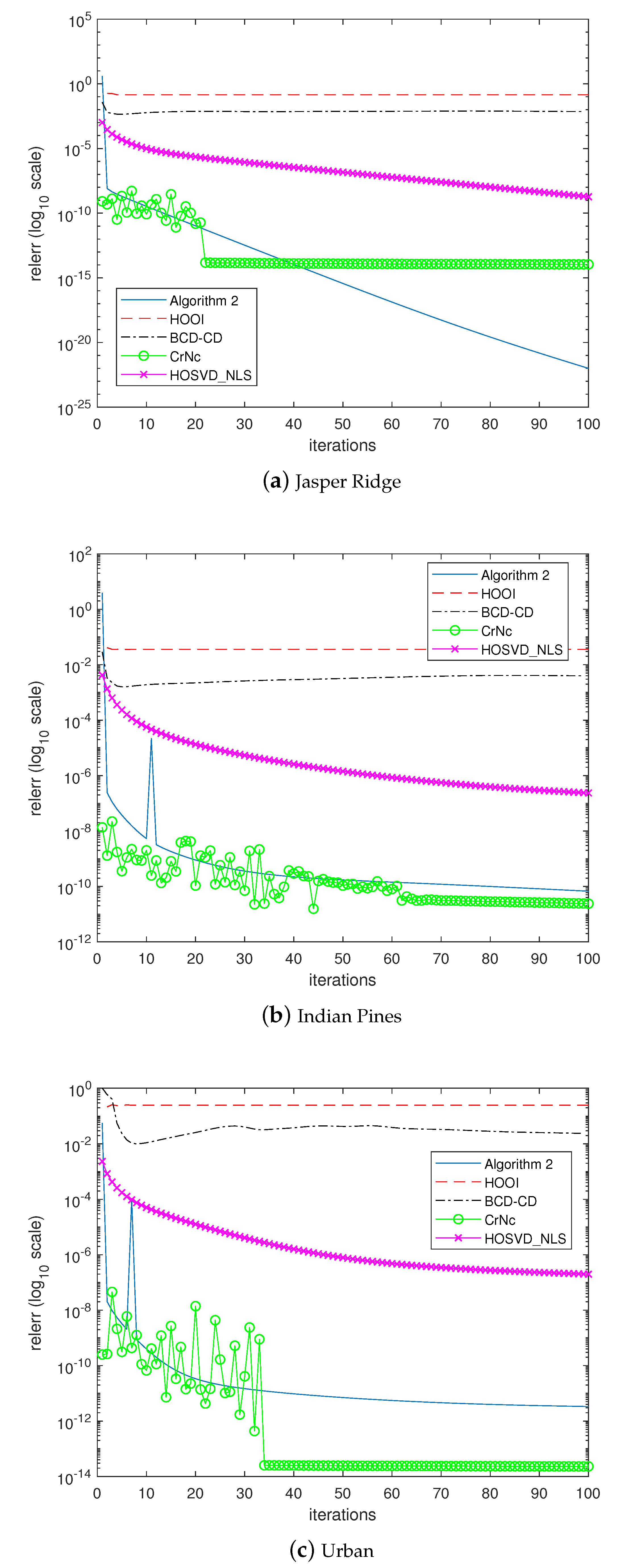
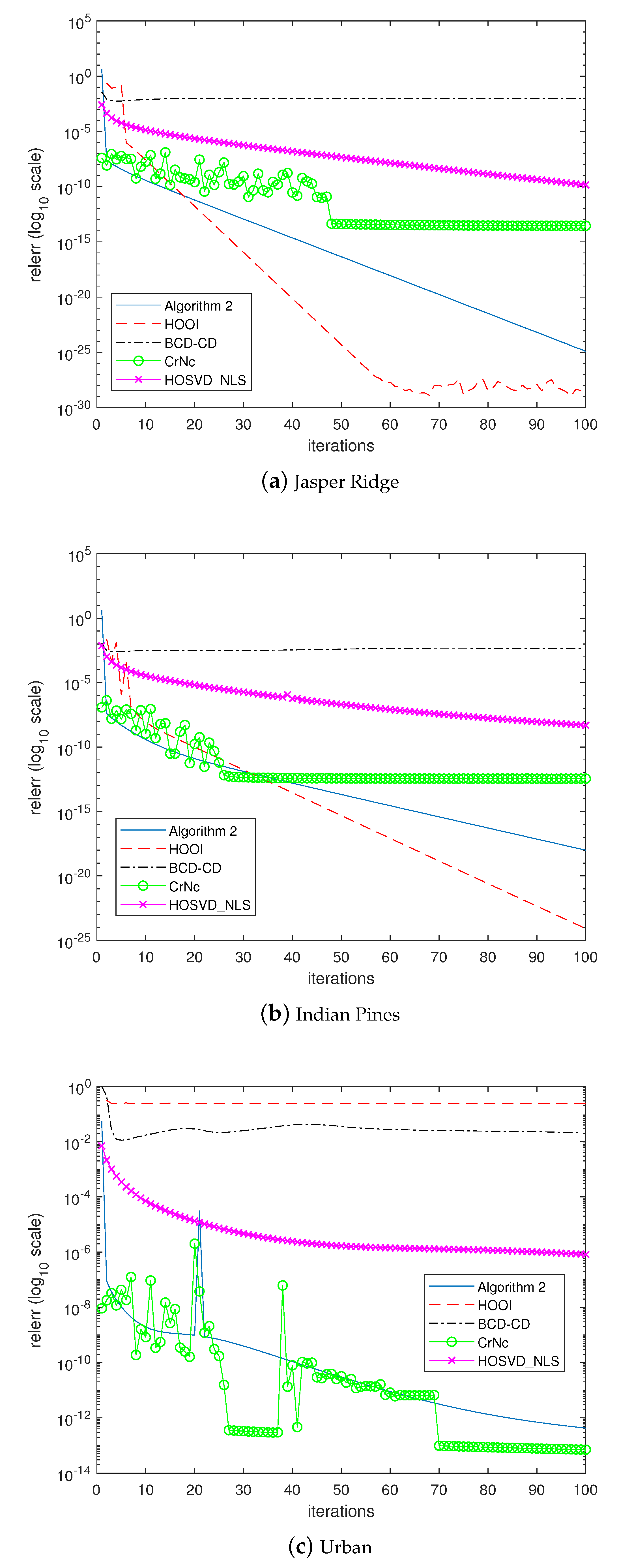
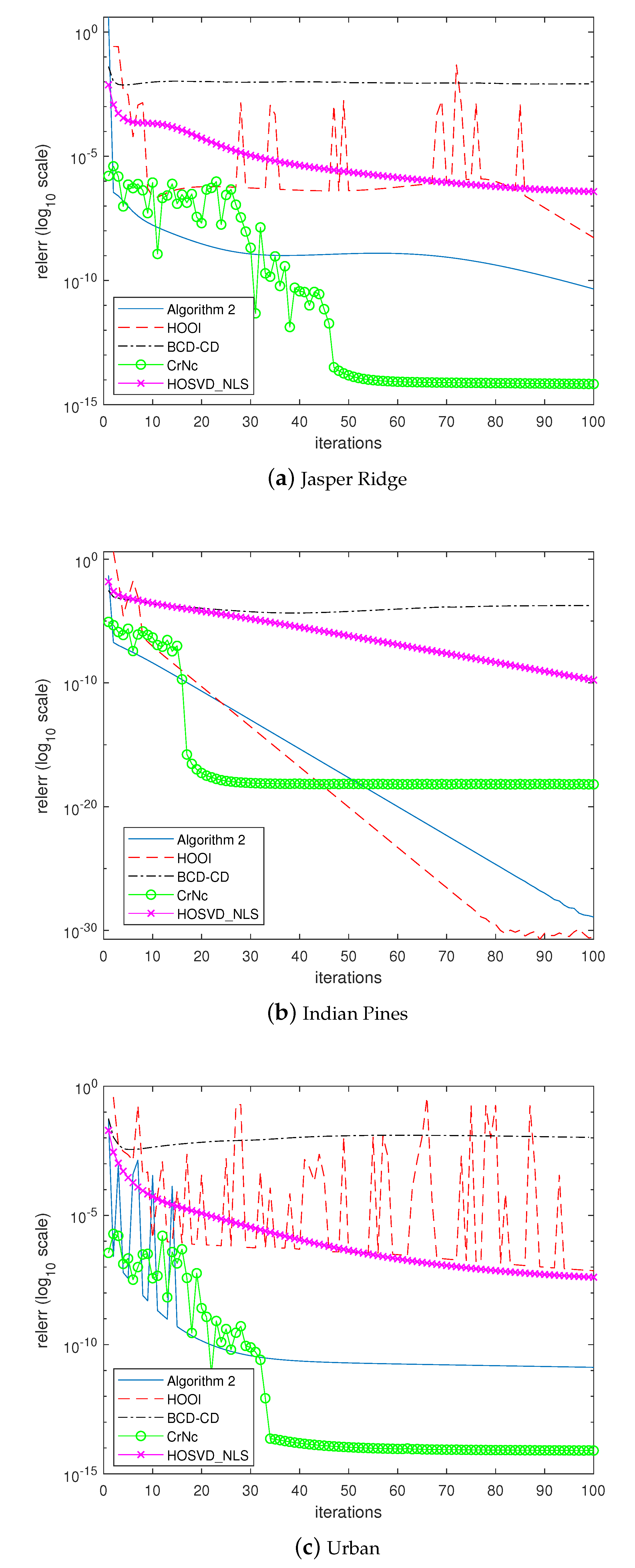
The last experiment examined how the algorithms would converge to the solutions. In the experiment, the algorithms were forced to continue until 100 iterations without considering the stopping criterion. Figure 5, Figure 6, Figure 7 and Figure 8 depict the histories of convergences when , , , , respectively. Additionally, Table 9 shows the relative errors of outputs after the iterations reached 100 steps. In this experiment, even though the overall shapes of convergence histories from CrNc appear better than the others, the outputs of CrNc seem to converge to the relatively inaccurate local minimum, as shown in Table 9. The convergence speed of HOSVD_NLS is very slow according to this experiment, but no-meaningful differences with HOOI in terms accuracy were generated. Furthermore, HOOI produces unstable convergence history occasionally. In any case, Algorithm 2 produces robust outputs with stable convergence histories and with the accuracy close to that of HOOI.
6. Conclusions
Hyperspectral imaging is widely used, as it enables the simultaneous manipulation of the spatial and spectral distribution information of a target scene. Owing to the massive amount of information, tensor compression techniques such as higher order singular value decomposition must be applied. In this paper, we suggested an efficient computation method of higher order singular value decomposition by using sequential computations of an alternating least squares approach. Experiments on real-world hyperspectral imaging datasets highlight the faster computation of the proposed algorithm with no-meaningful difference in accuracy compared to higher order orthogonal iteration, which is typically known as the most accurate algorithm for computing higher order singular value decomposition.
Funding
This work was supported by Hankuk University of Foreign Studies Research Fund and the National Research Foundation of Korea (NRF) grant funded by the Korean government (2018R1C1B5085022).
Conflicts of Interest
The author declares no conflict of interest.
References
- Bioucas-Dias, J.M.; Plaza, A.; Dobigeon, N.; Parente, M.; Du, Q.; Gader, P.; Chanussot, J. Hyperspectral Unmixing Overview: Geometrical, Statistical, and Sparse Regression-Based Approaches. IEEE Sel. Top. Appl. Earth Obs. Remote. Sen. 2012, 5, 354–379. [Google Scholar] [CrossRef] [Green Version]
- Grahn, H.; Geladi, P. Techniques and Applications of Hyperspectral Image Analysis; John Wiley & Sons: New York, NY, USA, 2007. [Google Scholar]
- Transon, J.; Andrimont, R.; Maugnard, A. Survey of Hyperspectral Earth Observation Applications from Space in the Sentinel-2 Context. Remote Sens. 2018, 10, 157. [Google Scholar] [CrossRef] [Green Version]
- Lu, G.; Fei, B. Medical hyperspectral imaging: A review. Biomed. Opt. 2014, 19, 1–23. [Google Scholar] [CrossRef] [PubMed]
- Lee, H.; Yang, C.; Kim, M.; Lim, J.; Cho, B.; Lefcourt, A.; Chao, K.; Everard, C. A Simple Multispectral Imaging Algorithm for Detection of Defects on Red Delicious Apples. J. Biosyst. Eng. 2014, 39, 142–149. [Google Scholar] [CrossRef]
- Nasrabadi, N.M. Hyperspectral Target Detection. IEEE Signal Process. Mag. 2013, 31, 34–44. [Google Scholar] [CrossRef]
- Poojary, N.; D’Souza, H.; Puttaswamy, M.R.; Kumar, G.H. Automatic target detection in hyperspectral image processing: A review of algorithms. In Proceedings of the 2015 12th International Conference on Fuzzy Systems and Knowledge Discovery (FSKD), Zhangjiajie, China, 15–17 August 2015; pp. 1991–1996. [Google Scholar]
- Renard, N.; Bourennane, S. Dimensionality Reduction Based on Tensor Modeling for Classification Methods. IEEE Trans. Geosci. Remote Sens. 2009, 47, 1123–1131. [Google Scholar] [CrossRef]
- Fang, L.; He, N.; Lin, H. CP tensor-based compression of hyperspectral images. J. Opt. Soc. Am. A Opt. Image Sci. Vis. 2017, 34, 252–258. [Google Scholar] [CrossRef] [PubMed]
- Yan, R.; Peng, J.; Wen, D.; Ma, D. Denoising and dimensionality reduction based on PARAFAC decomposition for hyperspectral imaging. Proc. SPIE Opt. Sens. Image. Tech. Appl. 2018, 10846, 538–549. [Google Scholar]
- Lathauwer, L.D.; Moor, B.D.; Vandewalle, J. A Multilinear Singular Value Decomposition. SIAM J. Matrix Anal. Appl. 2000, 21, 1253–1278. [Google Scholar] [CrossRef] [Green Version]
- Kolda, T.G.; Bader, B.W. Tensor Decomposition and Applications. Siam Rev. 2009, 51, 455–500. [Google Scholar] [CrossRef]
- Lathauwer, L.D.; Moor, B.D.; Vandewalle, J. On the Best Rank-1 and Rank-(R1, R2, …, RN) Approximation of Higher-Order Tensors. SIAM J. Matrix Anal. Appl. 2000, 21, 1324–1342. [Google Scholar] [CrossRef]
- Zhang, L.; Zhang, L.; Tao, D.; Huang, X.; Du, B. Compression of hyperspectral remote sensing images by tensor approach. Neurocomputing 2015, 147, 358–363. [Google Scholar] [CrossRef]
- An, J.; Lei, J.; Song, Y.; Zhang, X.; Guo, J. Tensor Based Multiscale Low Rank Decomposition for Hyperspectral Images Dimensionality Reduction. Remote Sens. 2019, 11–12, 1485. [Google Scholar] [CrossRef] [Green Version]
- Eldén, L.; Savas, B. A Newton-Grassmann method for computing the Best Multi-Linear Rank-(r1, r2, r3) Approximation of a Tensor. Siam Matrix Anal. Appl. 2009, 31, 248–271. [Google Scholar] [CrossRef] [Green Version]
- Sorber, L.; Barel, M.V.; Lathauwer, L.D. Structured Data Fusion. IEEE Sel. Top. Sig. Proc. 2015, 9, 586–600. [Google Scholar] [CrossRef]
- Hassanzadeh, S.; Karami, A. Compression and noise reduction of hyperspectral images using non-negative tensor decomposition and compressed sensing. Eur. J. Remote Sens. 2016, 49, 587–598. [Google Scholar] [CrossRef]
- Phan, A.; Cichocki, A.; Tichavsky, P. On Fast Algorithms for Orthogonal Tucker Decomposition. In Proceedings of the 2014 IEEE International Conference on Acoustics, Speech and Signal Processing (ICASSP), Florence, Italy, 4–9 May 2014; pp. 6766–6770. [Google Scholar]
- Lee, G. Fast computation of the compressive hyperspectral imaging by using alternating least squares methods. Sig. Proc. Image Commun. 2018, 60, 100–106. [Google Scholar] [CrossRef]
- Zhu, F.; Wang, Y.; Xiang, S.; Fan, B.; Pan, C. Structured Sparse Method for Hyperspectral Unmixing. ISPRS J. Photogramm. Remote Sens. 2014, 88, 101–118. [Google Scholar] [CrossRef] [Green Version]
- Baumgardner, M.F.; Biehl, L.L.; Landgrebe, D.A. 220 Band AVIRIS Hyperspectral Image Data Set: June 12, 1992 Indian Pine Test Site 3. Purdue Univ. Res. Repos. 2015, 10, R7RX991C. [Google Scholar]
- Xu, Y.; Yin, W. A Block Coordinate Descent Method for Regularized Multiconvex Optimization with Applications to Nonnegative Tensor Factorization and Completion. Siam Imag. Sci. 2013, 6, 1758–1789. [Google Scholar] [CrossRef]
- Vervliet, N.; Devals, O.; Sorber, L.; Van Barel, M.; De Lathauwer, L. Tensorlab 3.0. Available online: https://www.tensorlab.net/ (accessed on 10 March 2016).
Figure 1.
Example of third order tensor matricization along each mode.

Figure 2.
Sequential computations of factor matrices from Tucker-1 model optimization problems.

Figure 3.
Real-world HSI dataset for performance comparison of the proposed algorithm. Images display the average intensities of pixels throughout the spectrum.
Figure 3.
Real-world HSI dataset for performance comparison of the proposed algorithm. Images display the average intensities of pixels throughout the spectrum.

Figure 4.
The first channel image of compressed HSI when the Jasper Ridge dataset was used; dB, , and .
Figure 4.
The first channel image of compressed HSI when the Jasper Ridge dataset was used; dB, , and .

Figure 5.
Convergence history of the algorithms when .

Figure 6.
Convergence history of the algorithms when .

Figure 7.
Convergence history of the algorithms when .

Figure 8.
Convergence history of the algorithms when .


Table 1.
Multilinear ranks of the initial factor matrices computed from HOSVD when , and , respectively.
Table 1.
Multilinear ranks of the initial factor matrices computed from HOSVD when , and , respectively.
| Dataset | 0.1 | 0.2 | 0.3 | |
|---|---|---|---|---|
| Jasper Ridge | (71,75,5) | (48,54,3) | (28,32,2) | (17,20,2) |
| Indian Pines | (97,117,8) | (44,51,2) | (11,10,2) | (3,3,2) |
| Urban | (292,227,13) | (265,165,5) | (186,93,3) | (108,52,3) |
Table 2.
Experimental results of algorithms when the Jasper Ridge dataset was used and .
| HOOI | CrNc | HOSVD_NLS | BCD-CD | Algorithm 2 | ||
|---|---|---|---|---|---|---|
| 0.05 | iteration | 100 | 2 | 29 | 100 | 2 |
| relerr | 0.0291179 | 0.0291398 | 0.0291181 | 0.155959 | 0.0291264 | |
| time (s) | 8.1602 | 0.2674 | 8.3305 | 4.6889 | 0.1905 | |
| 0.1 | iteration | 5 | 2 | 26 | 100 | 2 |
| relerr | 0.0591755 | 0.0592419 | 0.0591757 | 0.152589 | 0.0591861 | |
| time (s) | 0.3509 | 0.2197 | 4.4906 | 3.4722 | 0.1401 | |
| 0.2 | iteration | 8 | 4 | 68 | 100 | 6 |
| relerr | 0.118573 | 0.118831 | 0.118572 | 0.161462 | 0.118703 | |
| time (s) | 0.4058 | 0.2921 | 6.3683 | 2.4399 | 0.2031 | |
| 0.3 | iteration | 6 | 6 | 23 | 100 | 6 |
| relerr | 0.141258 | 0.141271 | 0.141258 | 0.179646 | 0.141280 | |
| time (s) | 0.2339 | 0.2978 | 1.9192 | 3.4341 | 0.1442 |
Table 3.
Experimental results of algorithms when the Indian Pines dataset was used and .
| HOOI | CrNc | HOSVD_NLS | BCD-CD | Algorithm 2 | ||
|---|---|---|---|---|---|---|
| 0.05 | iteration | 100 | 2 | 57 | 100 | 4 |
| relerr | 0.0303899 | 0.0304928 | 0.0303906 | 0.071481 | 0.0303906 | |
| time (s) | 20.6298 | 0.5488 | 45.4292 | 12.0304 | 0.7744 | |
| 0.1 | iteration | 6 | 2 | 36 | 100 | 2 |
| relerr | 0.0527313 | 0.0528268 | 0.0527315 | 0.073079 | 0.0527553 | |
| time (s) | 0.6524 | 0.2927 | 7.5470 | 4.6133 | 0.2011 | |
| 0.2 | iteration | 7 | 4 | 48 | 100 | 6 |
| relerr | 0.0768619 | 0.0770075 | 0.0768605 | 0.124355 | 0.0769648 | |
| time (s) | 0.2839 | 0.2696 | 6.1851 | 2.0955 | 0.1630 | |
| 0.3 | iteration | 2 | 2 | 9 | 50 | 2 |
| relerr | 0.105915 | 0.105915 | 0.105915 | 0.127037 | 0.105915 | |
| time (s) | 0.0814 | 0.1522 | 1.1482 | 0.6996 | 0.0662 |
Table 4.
Experimental results of algorithms when the Urban dataset was used and .
| HOOI | CrNc | HOSVD_NLS | BCD-CD | Algorithm 2 | ||
|---|---|---|---|---|---|---|
| 0.05 | iteration | 100 | 2 | 47 | 100 | 2 |
| relerr | 0.0310416 | 0.0311142 | 0.0310424 | 0.298475 | 0.0310626 | |
| time (s) | 84.2434 | 1.8922 | 303.6298 | 63.0052 | 1.9077 | |
| 0.1 | iteration | 100 | 2 | 91 | 100 | 5 |
| relerr | 0.0617698 | 0.0621153 | 0.0617709 | 0.290838 | 0.0617950 | |
| time (s) | 63.7905 | 1.5078 | 242.1523 | 45.4830 | 2.9882 | |
| 0.2 | iteration | 12 | 4 | 42 | 100 | 6 |
| relerr | 0.120992 | 0.121752 | 0.120992 | 0.299642 | 0.12102 | |
| time (s) | 4.7328 | 1.8160 | 39.5247 | 27.2452 | 1.8032 | |
| 0.3 | iteration | 12 | 6 | 44 | 100 | 8 |
| relerr | 0.180622 | 0.181341 | 0.180624 | 0.295660 | 0.180645 | |
| time (s) | 3.0067 | 1.7068 | 27.0944 | 1.8032 | 27.2452 |
Table 5.
Experimental results of algorithms when Jasper Ridge dataset was used and .
| HOOI | CrNc | HOSVD_NLS | BCD-CD | Algorithm 2 | ||
|---|---|---|---|---|---|---|
| 0.05 | iteration | 100 | 2 | 81 | 100 | 6 |
| relerr | 0.0291179 | 0.0291398 | 0.0291179 | 0.155959 | 0.0291195 | |
| time (s) | 8.1761 | 0.2747 | 22.4445 | 4.7015 | 0.4218 | |
| 0.1 | iteration | 10 | 2 | 63 | 100 | 11 |
| relerr | 0.0591755 | 0.0592419 | 0.0591755 | 0.152589 | 0.0591765 | |
| time (s) | 0.6939 | 0.2399 | 10.3936 | 3.4566 | 0.5311 | |
| 0.2 | iteration | 97 | 6 | 100 | 100 | 39 |
| relerr | 0.118564 | 0.118782 | 0.118571 | 0.174686 | 0.118575 | |
| time (s) | 4.4129 | 0.6047 | 9.3648 | 2.4832 | 1.1770 | |
| 0.3 | iteration | 9 | 15 | 39 | 100 | 15 |
| relerr | 0.141258 | 0.141259 | 0.141258 | 0.179646 | 0.141259 | |
| time (s) | 0.3618 | 0.5357 | 3.1429 | 1.8633 | 0.3152 |
Table 6.
Experimental results of algorithms when Indian Pines dataset was used and .
| HOOI | CrNc | HOSVD_NLS | BCD-CD | Algorithm 2 | ||
|---|---|---|---|---|---|---|
| 0.05 | iteration | 100 | 2 | 100 | 100 | 14 |
| relerr | 0.0303899 | 0.0304928 | 0.0303903 | 0.071481 | 0.0303932 | |
| time (s) | 20.4660 | 0.5455 | 79.4811 | 11.8359 | 2.5751 | |
| 0.1 | iteration | 9 | 8 | 89 | 100 | 12 |
| relerr | 0.0527312 | 0.0527693 | 0.0527312 | 0.073079 | 0.0527339 | |
| time (s) | 0.9499 | 0.9088 | 18.6477 | 4.6742 | 0.8240 | |
| 0.2 | iteration | 12 | 16 | 76 | 100 | 27 |
| relerr | 0.0768604 | 0.0768700 | 0.0768604 | 0.124355 | 0.0768864 | |
| time (s) | 0.4698 | 0.8457 | 9.6352 | 2.1600 | 0.5941 | |
| 0.3 | iteration | 4 | 4 | 18 | 100 | 6 |
| relerr | 0.105915 | 0.105915 | 0.105915 | 0.126850 | 0.105915 | |
| time (s) | 0.1358 | 0.2284 | 2.2056 | 1.3507 | 0.1252 |
Table 7.
Experimental results of algorithms when Urban dataset was used and .
| HOOI | CrNc | HOSVD_NLS | BCD-CD | Algorithm 2 | ||
|---|---|---|---|---|---|---|
| 0.05 | iteration | 100 | 2 | 100 | 100 | 9 |
| relerr | 0.0310416 | 0.0311142 | 0.0310421 | 0.298475 | 0.0310468 | |
| time (s) | 84.8450 | 1.9226 | 665.8282 | 63.4775 | 6.4988 | |
| 0.1 | iteration | 100 | 8 | 100 | 100 | 18 |
| relerr | 0.0617698 | 0.0620033 | 0.0617706 | 0.290838 | 0.0617754 | |
| time (s) | 64.3367 | 5.3712 | 268.656 | 45.8471 | 9.2198 | |
| 0.2 | iteration | 100 | 13 | 100 | 100 | 24 |
| relerr | 0.120991 | 0.121355 | 0.120993 | 0.299642 | 0.120993 | |
| time (s) | 39.3584 | 5.5898 | 95.7108 | 27.6234 | 6.8905 | |
| 0.3 | iteration | 38 | 13 | 100 | 100 | 27 |
| relerr | 0.180622 | 0.180855 | 0.180622 | 0.29566 | 0.180625 | |
| time (s) | 9.5898 | 3.5682 | 61.3466 | 16.7007 | 4.4569 |
Table 8.
Experimental results of algorithms when HSI dataset when Gaussian white noise was used and . The numbers in the parenthesis represent the average iteration numbers.
Table 8.
Experimental results of algorithms when HSI dataset when Gaussian white noise was used and . The numbers in the parenthesis represent the average iteration numbers.
| Dataset | HOOI | CrNc | HOSVD_NLS | BCD-CD | Algorithm 2 | ||
|---|---|---|---|---|---|---|---|
| Jasper Ridge | 0.1 | +60 dB | 0.0591755 (5) | 0.0592419 (2) | 0.0591757 (26) | 0.153469 (100) | 0.0591861 (2) |
| +30 dB | 0.0449392 (100) | 0.0449707 (2) | 0.0449392 (25.33) | 0.152897 (100) | 0.0449440 (2.67) | ||
| +20 dB | 0.0788476 (100) | 0.0788524 (2) | 0.0788469 (100) | 0.118547 (100) | 0.0788477 (2.67) | ||
| 0.3 | +60 dB | 0.141258 (5.67) | 0.141296 (5.17) | 0.141258 (23) | 0.179359 (100) | 0.141280 (6) | |
| +30 dB | 0.137677 (5.83) | 0.137713 (4.67) | 0.137677 (24.33) | 0.175483 (100) | 0.137699 (5) | ||
| +20 dB | 0.113076 (6.33) | 0.113200 (2.83) | 0.113077 (32.5) | 0.166953 (100) | 0.113094 (4.33) | ||
| Indian Pines | 0.1 | +60 dB | 0.0527313 (6.33) | 0.0528347 (2) | 0.0527315 (36) | 0.0731127 (100) | 0.0527554 (2) |
| +30 dB | 0.0491485 (6.83) | 0.0492972 (2) | 0.0491491 (100) | 0.0739519 (100) | 0.0491542 (5.16) | ||
| +20 dB | 0.0791087 (100) | 0.0790856 (2) | 0.0790949 (100) | 0.0962606 (100) | 0.0790843 (2.83) | ||
| 0.3 | +60 dB | 0.105915 (2) | 0.105915 (2) | 0.105915 (9) | 0.127037 (50) | 0.105915 (2) | |
| +30 dB | 0.1053231 (2.67) | 0.103234 (2) | 0.103231 (11) | 0.124117 (100) | 0.103233 (5) | ||
| +20 dB | 0.0618722 (7.33) | 0.0620632 (2.5) | 0.0618740 (41.83) | 0.0746809 (100) | 0.0619321 (2.33) | ||
| Urban | 0.1 | +60 dB | 0.0617699 (100) | 0.0621156 (2) | 0.0617710 (90.67) | 0.289897 (100) | 0.0618057 (5) |
| +30 dB | 0.0539840 (71.67) | 0.0543273 (2) | 0.0539852 (52.33) | 0.296169 (100) | 0.0540272 (4.5) | ||
| +20 dB | 0.0853106 (70.67) | 0.08527384 (2) | 0.0853042 (100) | 0.302653 (100) | 0.0852731 (2.83) | ||
| 0.3 | +60 dB | 0.180622 (13) | 0.181286 (5.83) | 0.180624 (43.5) | 0.295660 (100) | 0.180645 (8) | |
| +30 dB | 0.178234 (12.83) | 0.179252 (4.33) | 0.178236 (36.17) | 0.298176 (100) | 0.178262 (5.5) | ||
| +20 dB | 0.158404 (68.33) | 0.159271 (2) | 0.158406 (20.83) | 0.297824 (100) | 0.158410 (7.16) |
Table 9.
Relative errors when algorithms continue for 100 iterations.
| HOOI | CrNc | HOSVD_NLS | BCD-CD | Algorithm 2 | ||
|---|---|---|---|---|---|---|
| 0.05 | Jasper Ridge | 0.0291179 | 0.0291283 | 0.0291179 | 0.155959 | 0.0291179 |
| Indian Pines | 0.033899 | 0.0304179 | 0.0303900 | 0.071481 | 0.0303903 | |
| Urban | 0.0310416 | 0.0310716 | 0.0310418 | 0.298475 | 0.0310421 | |
| 0.1 | Jasper Ridge | 0.0591755 | 0.0591779 | 0.0591755 | 0.152589 | 0.0591755 |
| Indian Pines | 0.0527312 | 0.0527466 | 0.0527312 | 0.073079 | 0.0527312 | |
| Urban | 0.0617698 | 0.0618683 | 0.0617698 | 0.290838 | 0.0617706 | |
| 0.2 | Jasper Ridge | 0.118564 | 0.118621 | 0.118564 | 0.161462 | 0.118571 |
| Indian Pines | 0.0768604 | 0.0768700 | 0.0768604 | 0.124355 | 0.0768604 | |
| Urban | 0.120991 | 0.121298 | 0.120991 | 0.299642 | 0.120992 | |
| 0.3 | Jasper Ridge | 0.141258 | 0.141258 | 0.141258 | 0.179646 | 0.141258 |
| Indian Pines | 0.105915 | 0.105915 | 0.105915 | 0.126850 | 0.105915 | |
| Urban | 0.180622 | 0.180855 | 0.180622 | 0.295660 | 0.180622 |
© 2019 by the author. Licensee MDPI, Basel, Switzerland. This article is an open access article distributed under the terms and conditions of the Creative Commons Attribution (CC BY) license (http://creativecommons.org/licenses/by/4.0/).
Share and Cite
MDPI and ACS Style
Lee, G. An Efficient Compressive Hyperspectral Imaging Algorithm Based on Sequential Computations of Alternating Least Squares. Remote Sens. 2019, 11, 2932. https://doi.org/10.3390/rs11242932
AMA Style
Lee G. An Efficient Compressive Hyperspectral Imaging Algorithm Based on Sequential Computations of Alternating Least Squares. Remote Sensing. 2019; 11(24):2932. https://doi.org/10.3390/rs11242932
Chicago/Turabian StyleLee, Geunseop. 2019. "An Efficient Compressive Hyperspectral Imaging Algorithm Based on Sequential Computations of Alternating Least Squares" Remote Sensing 11, no. 24: 2932. https://doi.org/10.3390/rs11242932
Note that from the first issue of 2016, this journal uses article numbers instead of page numbers. See further details here.