A Novel Method for the Absolute Pose Problem with Pairwise Constraints

Abstract

Absolute pose estimation from corrupted point correspondences is typically a problem of estimating parameters from outlier-contaminated data. Conventionally, for a fixed dimensionality d and the number of measurements N, a robust estimation problem cannot be solved exactly faster than $\mathcal{O}\left(N^d\right)$. Furthermore, it is almost impossible to remove d from the exponent of the runtime of a globally optimal algorithm. However, absolute pose estimation is a geometric parameter estimation problem, and thus has special constraints. In this paper, we consider pairwise constraints and propose a novel algorithm utilizing global optimization method Branch-and-Bound (BnB) for solving the absolute pose estimation problem. Concretely, we first decouple the rotation and the translation subproblems by utilizing the pairwise constraints, and then we solve the rotation subproblem using the BnB algorithm. Lastly, we estimate the translation based on the optimal rotation by using another BnB algorithm. The proposed algorithm has an approximately linear complexity in the number of correspondences at a given outlier ratio. The advantages of our method were demonstrated via thorough testing on both synthetic and real-world data.

1. Introduction

Camera pose estimation is a critical and fundamental problem in computer vision [1], robotics [2], photogrammetry [3,4], and many other related areas. The problem of estimating the absolute pose of a calibrated camera given a certain number of correspondences between 3D world points and 2D image projection points is known as the Perspective-n-Point (PnP) problem [5]. It arises as a subtask in many different applications (e.g., robot vision navigation [6], camera localization [7], and generation of digital heritage [8,9]).

Solving PnP problem has been studied for many years and various methods have been proposed [10]. However, in practical applications, these PnP methods cannot work independently because of mismatches in point-to-point correspondences [11]. These mismatches are called outliers and the corrupted point-to-point correspondences are called outlier-contaminated data. Solving PnP problems with outliers are, therefore, highly needed in real applications [12]. Although some methods are proposed to solve the problem, a more robust method is still needed.

Mathematically, the absolute pose estimation problem, i.e., the problem of estimating the pose parameters (rotation and translation) given certain observations (3D points and 2D points), is a typical parameter estimation problem [13] (also a fitting problem [14]). This problem has been studied for more than a century, and researchers have proposed many methods [15,16,17,18] to improve the solution speed, accuracy, and robustness to outliers. However, a recent study [19] has shown that fitting a model to data with outliers is an NP-hard problem. A somewhat promising result is that, for a fixed dimensionality d, a robust estimation problem can be solved in polynomial time in the number of measurements N [20]. However, this does not imply that a generalized robust estimation problem with outliers can be solved efficiently because a generalized robust fitting problem is a W[1]-hard problem in d dimensions [19] and, more specifically, it cannot be solved faster than $\mathcal{O}\left(N^d\right)$ [17,21]. Furthermore, it is almost impossible to remove d from the exponent of the run time of a globally optimal algorithm [19].

In addition, we can show the “hardness” of the absolute pose estimation with corrupted data from the optimization perspective. Generally, a robust absolute pose estimation problem is always a nonconvex optimization problem [13,16]. There are two reasons robust absolute pose estimation must be formulated as a “hard” problem. One reason is that the non-convex objective functions are usually applied to suppress outliers. The other reason is that the robust estimation problem is optimized in $SE\left(3\right)$, which corresponds to two totally different manifolds, rotation ($\mathbf{R}\in SO\left(3\right)$) and translation ($\mathbf{t}\in {\mathbb{R}}^3)$). Although there are already some solid theories regarding convex optimization in ${\mathbb{R}}^3$ [22] and $SO\left(3\right)$ [23] separately, robust estimation in $SE\left(3\right)$ still seems to be a difficult problem [16].

In other words, when there are mismatches in the 2D–3D correspondences, the absolute pose estimation problem is a rather “hard” problem. However, in practical applications, outliers are inevitable and will lead to a significant decrease in accuracy for pose estimation [11]. Fortunately, the absolute pose estimation problem is a geometric fitting problem and thus may be efficiently solved by considering geometric constraints.

In this paper, we decouple the rotation and translation subproblems using pairwise constraints, thus reducing the dimensionality of the original problem. That is to say, the original six-degree-of-freedom (6-DoF) pose estimation problem is transformed into two 3-DoF subproblems, thereby significantly reducing the hardness of the pose estimation problem. The two subproblems are solved sequentially using Branch-and-Bound (BnB) algorithm and the obtained rotation and translation are globally optimal to their corresponding subproblems. As a result, we can efficiently obtain an optimal joint solution to the robust pose estimation problem.

Contributions of This Paper. In this paper, we introduce a novel robust and global solution to the absolute pose estimation problem, called Robust and Global PnP (RGPnP). As its name suggests, our proposed method is more robust than existing methods, since we apply global optimization methods to solve subproblems. The contributions are as follows:

• We use novel pairwise constraints to decouple the rotation and translation subproblems, which can then be efficiently solved sequentially. The dimensionality of the two subproblems are lower than that of the original problem; therefore, searching the exact solution of each subproblem is easier than searching the exact solution of the original problem.
• The proposed method is more robust than very recent heuristic methods [11]. The decoupled subproblems are solved by applied BnB algorithm, which is a global optimization algorithm, to obtain the globally optimal rotation and translation to their corresponding subproblems.

Note that, even though the obtained optimal rotation and translation are not necessarily globally optimal to the joint problem, our proposed method still obtains a satisfactory solution, which is more robust than existing heuristic methods, in real applications. Besides, the decoupling scheme contributes by reducing the computational complexity of BnB significantly.

2. Related Work

The camera pose problem has been studied for more than a century, and there is a large body of literature on the absolute pose estimation problem [10]. Here, we first review the PnP algorithm without mismatches. When the observations include no outliers, the PnP problem has a closed solution ($n\ge 3$). To reduce the sensitivity to noise and consider a larger point set, the Efficient PnP (EPnP) [5], Optimal PnP (OPnP) [24], and Unified PnP (UPnP) [25] methods have been developed to produce accurate results with a linear complexity. These algorithms are applied in many related areas and can be regarded as state-of-the-art outlier-free PnP techniques.

When the observations include outliers, the most commonly applied mechanism is RANdom SAmple Consensus (RANSAC) [26,27], which is a well-known algorithm for robust parameters estimation that is widely used for the camera pose estimation problem. However, as its name suggests, it is a nondeterministic heuristic algorithm, which means that RANSAC lacks absolute certainty that the obtained solution is optimal. In other words, the solution of RANSAC is sub-optimal [17,28]. The most recent advancement is to remove outliers before applying an outlier-free PnP method. In the Robust Efficient Procrustes PnP method (REPPnP) [29], the pose estimation problem is formulated as a low-rank homogeneous system, and outliers are iteratively removed under the assumption that the rank of the null space of the linear system should always be one. Re-weighting and 1-Point RANSAC-based PnP (R1PPnP) [11] uses a heuristic method of handling outliers by utilizing a soft reweighting mechanism and the 1-point RANSAC scheme. However, the outlier removal problem is as hard as the original problem. Nevertheless, although it is difficult to eliminate all outliers efficiently, the proportion of outliers in the observations can be reduced using these outlier removal methods. Moreover, in practical applications, it may be possible to obtain prior knowledge that can be used in outlier removal. For example, Camposeco et al. [30] presented an outlier filter that incorporates prior information on the viewing directions, Svarm et al. [12] presented an approximate outlier rejection scheme with a known vertical direction, and the method proposed in [31] requires knowledge about the overall camera orientation with which to prune outliers.

In addition to the PnP methods discussed above, there is another class of methods for solving the robust pose estimation problem. In this body of work, the pose estimation problem is formulated as a robust optimization problem. M-estimator [10] is a classical robust estimation method, but it always solves to a local optimum because of the nonconvexity of the objective function. Therefore, more recent work on robust estimation has focused on obtaining globally optimal solutions. The most popular algorithm may be the Branch-and-Bound (BnB) algorithm, which is always combined with convex relaxation [16,32,33] or geometric relaxation [13,34]. However, the BnB-based algorithms devoted to pose estimation always suffer from a heavy computational burden for the obvious reason that the dimensionality of the feasible domain for pose estimation is six, and, thus, the pose estimation problem perhaps cannot be regarded as a low-dimensional optimization problem from the perspective of using BnB approach. In other words, even if the BnB algorithm has tight bounds, it still needs considerable time to search the entire feasible space in $SE\left(3\right)$. Moreover, the optimization is performed in two totally different manifolds, and it is not easy to calculate a tight bound for each branch.

Another topic that is closely related to the absolute pose estimation problem is point set registration [1,35]. Similarly, searching for globally optimal solutions is a hot topic in the field of point set registration, and the BnB algorithm has also been broadly applied in recent related studies. One of the most successful algorithms for this purpose may be the algorithm proposed in [36] and its subsequent versions [1,35,37]. These works are all based on rotation search theory, and, for $SE\left(3\right)$ optimization in particular, a more systematic scheme called the nested BnB is applied. Moreover, the decoupling method presented in [38] improves efficiency, which inspires us to decouple the rotation and translation subproblems by means of pairwise constraints.

3. Method

3.1. Problem Formulation

In this paper, we formulate the absolute pose estimation problem as follows. Let the ith 3D points in the world coordinate system be denoted by ${\mathit{p}}_i\in {\mathbb{R}}^3$, $i=1,\dots ,n$. Similarly, let ${\mathit{q}}_i\in {\mathbb{S}}^2$, $i=1,\dots ,n$ be the ith bearing vector with a unit norm, which corresponds to the ith 2D point in the camera coordinate system. $\mathbf{R}\in SO\left(3\right)$ is the rotation and $\mathbf{t}\in {\mathbb{R}}^3$ is the translation. Given these definitions, the relationship for inlier observation is as follows:

$${\lambda }_i{\mathit{q}}_i=\mathbf{R}{\mathit{p}}_i+\mathbf{t},i=1,\dots ,n$$

(1)

where ${\lambda }_i$ is the unknown depth of the ith point. The objective of the absolute pose estimation problem is then to estimate the rotation and translation, given n pairs of points. Alternatively, to eliminate ${\lambda }_i$, Equation (1) can be reformulated as follows:

$$\angle ({\mathit{q}}_i,\mathbf{R}{\mathit{p}}_i+\mathbf{t})=0$$

(2)

where $\angle (\mathit{a},\mathit{b})$ is the angle between vectors a and b. In this paper, we estimate the camera pose by maximizing the cardinality E of the inlier set ${\mathcal{S}}_I$:

$$E^{*}(\mathbf{R},\mathbf{t})=max\left|{\mathcal{S}}_I\right|$$

(3)

$${\mathcal{S}}_I=\left\{({\mathit{q}}_i,{\mathit{p}}_i)|\angle ({\mathit{q}}_i,\mathbf{R}{\mathit{p}}_i+\mathbf{t})<ϵ\right\}$$

(4)

where $ϵ$ is the inlier threshold.

The function given in Equation (4) is inherently robust to outliers since matched points are considered inliers only if their angular separation is below the inlier threshold $ϵ$. However, obtaining the global solution to Equation (3) is a nontrivial problem. We propose the use of a set of novel pairwise constraints to obtain an easier problem.

3.2. Eliminating Translation by Means of Pairwise Constraints

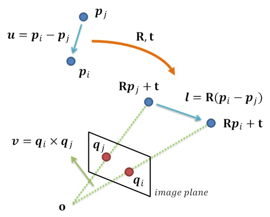
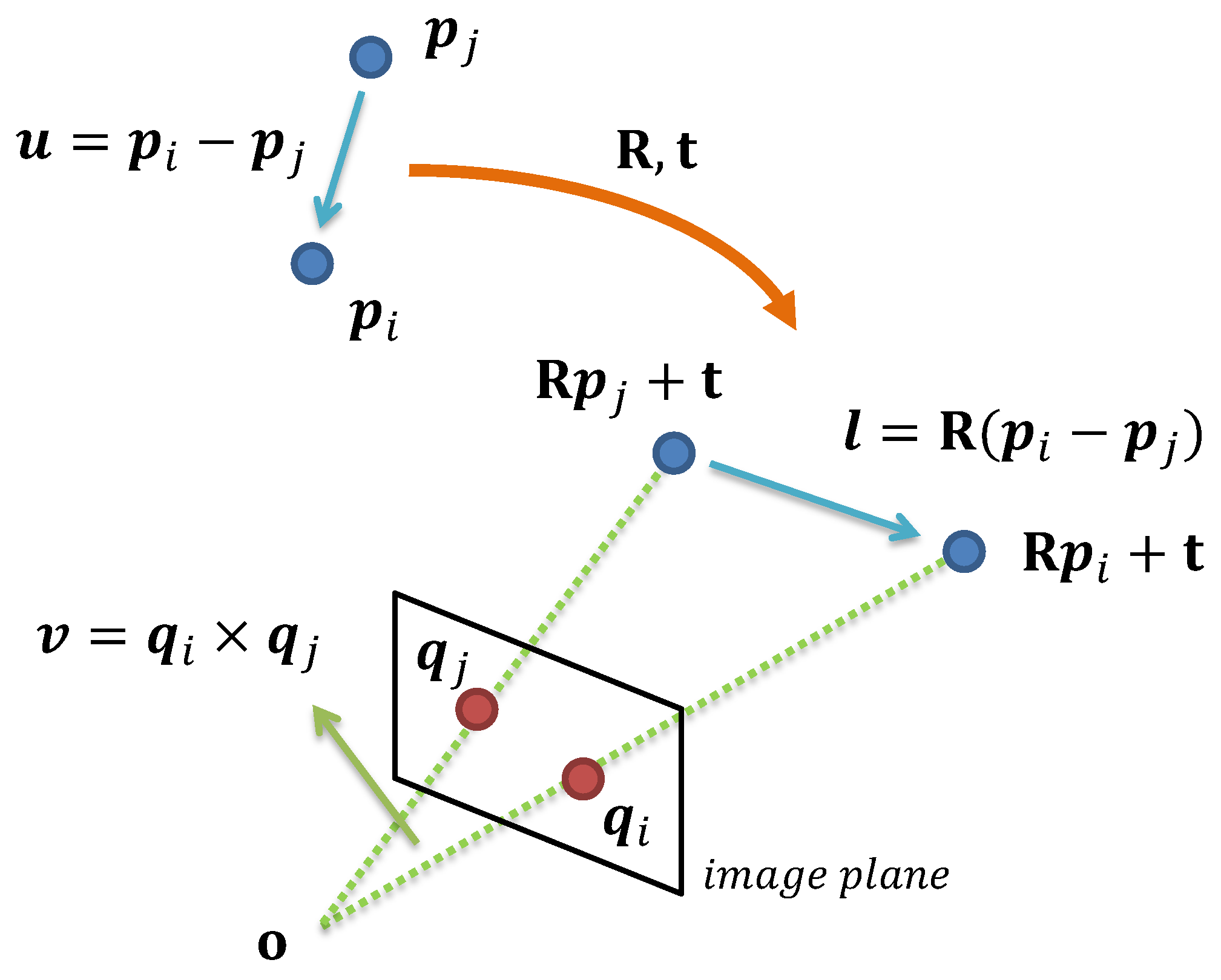
We consider two pairs of inlier correspondences $({\mathit{p}}_i,{\mathit{q}}_i)$ and $({\mathit{p}}_j,{\mathit{q}}_j)$. When they are aligned as shown in Figure 1, the four points and the center of the camera must all lie in the same plane. $\mathit{v}={\mathit{q}}_i\times {\mathit{q}}_j$ is the normal of that plane, and $\mathit{l}=(\mathbf{R}{\mathit{p}}_i+\mathbf{t})-(\mathbf{R}{\mathit{p}}_j+\mathbf{t})=\mathbf{R}({\mathit{p}}_i-{\mathit{p}}_j)$ is a vector in the plane. For simplicity, let $\mathit{u}={\mathit{p}}_i-{\mathit{p}}_j$; then, $\mathit{l}=\mathbf{R}\mathit{u}$. The relation between $\mathit{u}$ and $\mathit{v}$ is obvious: $\mathit{v}\perp \mathbf{R}\mathit{u}$ or ${\mathit{v}}^{\mathbf{T}}·\mathbf{R}\mathit{u}=0$, which is called a pairwise constraint in this paper (note that a similar equation was used by Ke and Roumeliotis [39]). Such pairwise constraints provide an easy and elegant yet powerful means of decoupling the rotation and translation in Equation (3); thus, we can calculate the optimal rotation first by enforcing these pairwise constraints. Consequently, we define a new objective function with only rotation parameters as follows:

$${\mathcal{Q}}^{*}\left(\mathbf{R}\right)=max\left|{\mathcal{S}}_I^p\right|$$

(5)

$${\mathcal{S}}_I^p=\left\{\left({\mathit{q}}_i,{\mathit{q}}_j,{\mathit{p}}_i,{\mathit{p}}_j\right)\left|\right|\angle \left({\mathit{q}}_i\times {\mathit{q}}_j,\mathbf{R}({\mathit{p}}_i-{\mathit{p}}_j)\right)-\frac{\pi }{2}|<\delta \right\}$$

(6)

where $i\ne j$ and $\delta$ is a new inlier threshold.

We can also use $(\mathit{u},\mathit{v})$ to rewrite Equation (5) as follows:

$${\mathcal{Q}}^{*}\left(\mathbf{R}\right)=max\sum _k\lfloor |\angle ({\mathit{v}}_k,\mathbf{R}{\mathit{u}}_k)-\frac{\pi }{2}|<\delta \rfloor$$

(7)

Here, $\lfloor ·\rfloor$ is a 0–1 function that returns a value of 1 if the condition is true and a value of 0 otherwise, and $k=1,\dots ,m$ is the index of the $(\mathit{u},\mathit{v})$ pairs.

We find that there is only the rotation to be solved for in Equation (7); thus, we have already successfully reduced the 6-DoF pose problem to a 3-DoF rotation estimation problem in $SO\left(3\right)$. However, the number of input data increases from n to 0.5 n$(n-1)$. In [40], the authors pointed out that estimated parameters can be found as a solution on a subset of all the input data. Unfortunately, the number of $(\mathit{u},\mathit{v})$ pairs is very large, and there are many different ways of choosing a subset from all samples. Nevertheless, for the absolute pose estimation problem, all original input observations are expected to be involved in the estimation to introduce redundancy and reduce the sensitivity to noise [5]. Interestingly, we find that, if each original point is used once, then the number of $(\mathit{u},\mathit{v})$ pairs decreases to 0.5 n under our pairwise constraints, as illustrated in Figure 2. Among the complete input, as long as we ensure that each original point is used only once, we can get the 0.5 n-subset, regardless of which two specific points are selected to make $\mathit{u}$ or $\mathit{v}$. It is worth pointing out that the 0.5 n-subset can be considered as the downsampling input of the complete 0.5 $n(n-1)$. If the outlier ratio is not very large, we recommend using this 0.5 n-subset as the input so that every original observation is involved in the estimation. However, if the outlier ratio is large, we recommend increasing the input size to have denser input.

3.3. Global SO(3) Search

In this section, we introduce a method based on the BnB algorithm for obtaining the global solution to Equation (7). We summarize the proposed method in Algorithm 1. In brief, the BnB algorithm proceeds by recursively subdividing and pruning the rotation space until the global optimum is found. In this paper, the rotation space $SO\left(3\right)$ is minimally parameterized with an angle-axis representation, and a 3D cube with a side length of 2 $\pi$ is used as the rotation domain. For more details about the angle-axis representation, please refer to [34].

Generally, the success of a BnB algorithm depends on the quality of its upper and lower bounds. In this paper, we present two different ways to calculate the bounds. The first pair of bounds is derived based on Hartley and Kahl’s rotation search theory. To obtain the second pair of bounds, the rotation matrix is stacked into a $9\times 1$ vector and Equation (7) is reformulated as a linear system.

Algorithm 1 BnB algorithm for obtaining the rotation.

Require: Correspondence pairs ${\left\{({\mathit{v}}_k,{\mathit{u}}_k)\right\}}_{k=1}^m$ and inlier threshold.

1: Initialize $\mathbb{B}\leftarrow$ cube of side length $2\pi$, and insert $\mathbb{B}$ into a priority queue q. 2: whileq is not empty do 3:  Subdivide $\mathbb{B}$ into eight cubes ${\left\{{\mathbb{B}}_d\right\}}_{d=1}^8$. 4:  For each ${\mathbb{B}}_d$ calculate the upper and lower bounds ${\left\{{\mathcal{Q}}_d^u,{\mathcal{Q}}_d^l\right\}}_{d=1}^8$, insert ${\mathbb{B}}_d$ with priority ${\mathcal{Q}}_d^u$ into q. 5:  Update the best solution so far: ${\mathcal{Q}}^{*}\left({\mathbf{R}}^{*}\right)=max\left\{{\mathcal{Q}}_i^l\right\}$, i for all branches. 6:  Remove the branches that ${\mathcal{Q}}_i^u<{\mathcal{Q}}^{*}$, i for all branches. 7:  Update the highest priority cube $\mathbb{B}$ with upper bound ${\mathcal{Q}}^u$ for the next loop. 8:  if ${\mathcal{Q}}^u={\mathcal{Q}}^{*}$ then 9:   terminate and return ${\mathbf{R}}^{*}$. 10:  end if 11: end while 12: return Optimal rotation ${\mathbf{R}}^{*}$.

3.3.1. Bounds from Hartley and Kahl’s Theory

Let us start with a famous equation that was proved in [34]. Given a cube-shaped branch $\mathbb{B}$ of the rotation space, whose center is ${\mathbf{R}}_0$, for any $\mathit{u}\in {\mathbb{R}}^3$ and any $\mathbf{R}\in \mathbb{B}$, the following holds:

$$\angle (\mathbf{R}\mathit{u},{\mathbf{R}}_0\mathit{u})\le \sqrt{3}\sigma$$

(8)

where $\sigma$ is the half-side length of the cube $\mathbb{B}$. According to the triangle inequality in a spherical geometry, for any $\mathit{v}\in {\mathbb{R}}^3$

$$\begin{array}{cc}\hfill \angle (\mathit{v},\mathbf{R}\mathit{u})& \le \angle (\mathit{v},{\mathbf{R}}_0\mathit{u})+\angle (\mathbf{R}\mathit{u},{\mathbf{R}}_0\mathit{u})\hfill \end{array}$$

(9)

$$\begin{array}{cc}\hfill & \le \angle (\mathit{v},{\mathbf{R}}_0\mathit{u})+\sqrt{3}\sigma \hfill \end{array}$$

(10)

$$\begin{array}{cc}\hfill \angle (\mathit{v},\mathbf{R}\mathit{u})& \ge \angle (\mathit{v},{\mathbf{R}}_0\mathit{u})-\angle (\mathbf{R}\mathit{u},{\mathbf{R}}_0\mathit{u})\hfill \end{array}$$

(11)

$$\begin{array}{cc}\hfill & \ge \angle (\mathit{v},{\mathbf{R}}_0\mathit{u})-\sqrt{3}\sigma \hfill \end{array}$$

(12)

From Equations (9)–(12), for a given pair $({\mathit{u}}_k,{\mathit{v}}_k)$, we can obtain

$$\begin{array}{cc}\hfill & |\angle ({\mathit{v}}_k,\mathbf{R}{\mathit{u}}_k)-\frac{\pi }{2}|\hfill \end{array}$$

(13)

$$\begin{array}{cc}\hfill & =|\angle ({\mathit{v}}_k,\mathbf{R}{\mathit{u}}_k)+\angle ({\mathit{v}}_k,{\mathbf{R}}_0{\mathit{u}}_k)-\angle ({\mathit{v}}_k,{\mathbf{R}}_0{\mathit{u}}_k)-\frac{\pi }{2}|\hfill \end{array}$$

(14)

$$\begin{array}{cc}\hfill & \ge |\angle ({\mathit{v}}_k,{\mathbf{R}}_0{\mathit{u}}_k)-\frac{\pi }{2}|-|\angle ({\mathit{v}}_k,\mathbf{R}{\mathit{u}}_k)-\angle ({\mathit{v}}_k,{\mathbf{R}}_0{\mathit{u}}_k)|\hfill \end{array}$$

(15)

$$\begin{array}{cc}\hfill & \ge |\angle ({\mathit{v}}_k,{\mathbf{R}}_0{\mathit{u}}_k)-\frac{\pi }{2}|-\sqrt{3}\sigma \hfill \end{array}$$

(16)

Then,

$$\lfloor |\angle ({\mathit{v}}_k,\mathbf{R}{\mathit{u}}_k)-\frac{\pi }{2}|<\delta \rfloor \le \lfloor |\angle ({\mathit{v}}_k,{\mathbf{R}}_0{\mathit{u}}_k)-\frac{\pi }{2}|-\sqrt{3}\sigma <\delta \rfloor$$

(17)

As a result, the upper bound of ${\mathcal{Q}}^{*}\left(\mathbf{R}\right)$ in Equation (7) for any $\mathbf{R}\in \mathbb{B}$ is

$${\mathcal{Q}}_H^{upper}\left(\mathbb{B}\right)=\sum _k\lfloor |\angle ({\mathit{v}}_k,{\mathbf{R}}_0{\mathit{u}}_k)-\frac{\pi }{2}|<\delta +\sqrt{3}\sigma \rfloor$$

(18)

The lower bound can be easily calculated as follows:

$${\mathcal{Q}}_H^{lower}\left(\mathbb{B}\right)=\sum _k\lfloor |\angle ({\mathit{v}}_k,{\mathbf{R}}_0{\mathit{u}}_k)-\frac{\pi }{2}|<\delta \rfloor$$

(19)

The proof for lower bound is obvious because no rotation in the branch can be better than the optimum.

3.3.2. Bounds Derived from A Linear System Formulation

From the equation ${\mathit{v}}^T·\mathbf{R}\mathit{u}=0$, we can obtain the linear homogeneous equation ${\mathit{e}}^T\mathit{x}=0$, where ${\mathit{x}}^T=({\mathbf{R}}_{1,1},{\mathbf{R}}_{2,1},\dots ,{\mathbf{R}}_{3,3})$ and ${\mathit{e}}^T=(v_1{u}_1,v_2{u}_1,\dots ,v_3{u}_3)$. Then, we have another orthogonal relation, $\angle (\mathit{e},\mathit{x})=\frac{\pi }{2}$, and we can reformulate Equation (7) as

$${\mathcal{Q}}^{*}\left(\mathbf{R}\right)=max\sum _k\lfloor |\angle ({\mathit{e}}_k,\mathit{x})-\frac{\pi }{2}|<\tau \rfloor$$

(20)

where $\tau$ is a different new inlier threshold. Notably, Equation (20) is the outlier-robust form of the linear system $E\mathit{x}=0$, where $E^T=({\mathit{e}}_1,{\mathit{e}}_2,\dots ,{\mathit{e}}_m)$.

To derive the upper bound of Equation (20), we introduce the famous Lemma 2 in [34], which states that the angular distance between two rotations is less than the Euclidean distance between them in the angle-axis representation:

$$\angle ({\mathbf{R}}_1,{\mathbf{R}}_2)\le \parallel {\mathit{r}}_1-{\mathit{r}}_2\parallel$$

(21)

where ${\mathbf{R}}_1$ and ${\mathbf{R}}_2$ are two rotations, while ${\mathit{r}}_1$ and ${\mathit{r}}_2$, respectively, are their angle-axis representations; $\angle ({\mathbf{R}}_1,{\mathbf{R}}_2)$ is the angle $\theta$ lying in the range $0\le \theta \le \pi$ of the rotation ${\mathbf{R}}_1^T{\mathbf{R}}_2$ (more details can be found in Section 3 of [34]). Additionally, according to Appendix A of [41],

$$trace\left({\mathbf{R}}_1^T{\mathbf{R}}_2\right)=1+2cos(\angle ({\mathbf{R}}_1,{\mathbf{R}}_2))$$

(22)

Meanwhile,

$$trace\left({\mathbf{R}}_1^T{\mathbf{R}}_2\right)={\mathit{x}}_1^T{\mathit{x}}_2$$

(23)

where ${\mathit{x}}_1$ and ${\mathit{x}}_2$ are the linear representations of ${\mathbf{R}}_1$ and ${\mathbf{R}}_2$, respectively. Then,

$$\begin{array}{cc}\hfill \angle ({\mathit{x}}_1,{\mathit{x}}_2)& =co{s}^{-1}\left(\frac{1}{\parallel {\mathit{x}}_1\parallel \parallel {\mathit{x}}_2\parallel }{\mathit{x}}_1^T{\mathit{x}}_2\right)\hfill \end{array}$$

(24)

$$\begin{array}{cc}\hfill & =co{s}^{-1}\left(\frac{1}{3}{\mathit{x}}_1^T{\mathit{x}}_2\right)\hfill \end{array}$$

(25)

where Equation (25) holds due to the fact that $\parallel {\mathit{x}}_1\parallel =\parallel {\mathit{x}}_2\parallel =\sqrt{3}$. With Equations (22) and (23), we can substitute ${\mathit{x}}_1^T{\mathit{x}}_2$ in Equation (25)

$$\begin{array}{cc}\hfill \angle ({\mathit{x}}_1,{\mathit{x}}_2)& =co{s}^{-1}\left(\frac{1}{3}trace\left({\mathbf{R}}_1^T{\mathbf{R}}_2\right)\right)\hfill \end{array}$$

(26)

$$\begin{array}{cc}\hfill & =co{s}^{-1}\left(\frac{1}{3}\left(1+2cos\left(\angle ({\mathbf{R}}_1,{\mathbf{R}}_2)\right)\right)\right)\hfill \end{array}$$

(27)

$$\begin{array}{cc}\hfill & \le co{s}^{-1}\left(\frac{1}{3}\left(1+2cos(\parallel {\mathit{r}}_1-{\mathit{r}}_2\parallel )\right)\right)\hfill \end{array}$$

(28)

where Equation (28) holds considering the inequality in Equation (21).

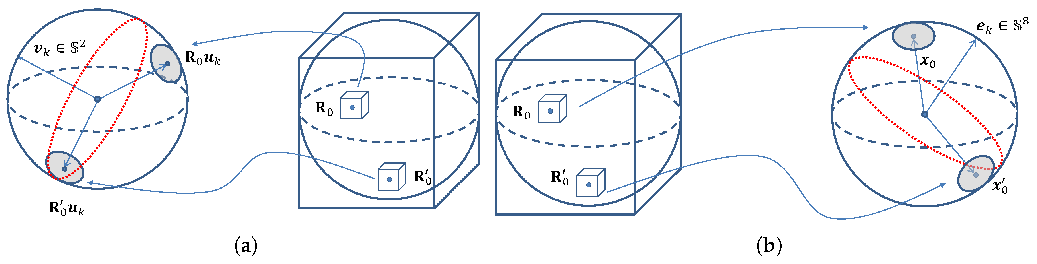
Equation (28) establishes a relation between the angle-axis representation and the linear representation. Geometrically, a cube-shaped branch in the angle-axis representation can be relaxed to a continuous region in the linear representation, as shown in Figure 3.

Specifically, in a cube-shaped branch $\mathbb{B}$ whose center is ${\mathbf{R}}_0$ (where ${\mathit{x}}_0$ and ${\mathit{r}}_0$ are the linear and angle-axis representations, respectively, of ${\mathbf{R}}_0$), for any $\mathbf{R}\in \mathbb{B}$,

$$\begin{array}{cc}\hfill \angle (\mathit{x},{\mathit{x}}_0)& \le co{s}^{-1}\left(\frac{1}{3}(1+2cos(\parallel \mathit{r}-{\mathit{r}}_0\parallel \left)\right)\right)\hfill \end{array}$$

(29)

$$\begin{array}{cc}\hfill & \le co{s}^{-1}\left(\frac{1}{3}\left(1+2cos\left(\sqrt{3}\sigma \right)\right)\right)=\alpha \hfill \end{array}$$

(30)

where $\mathit{x}$ and $\mathit{r}$ are the linear and angle-axis representations, respectively, of $\mathbf{R}$; $\sigma$ is the half-side length of the cube $\mathbb{B}$; and $\alpha$ denotes the upper bound of $\angle (\mathit{x},{\mathit{x}}_0)$. Similar to the first bound (Equations (9)–(12)), we have

$$\angle ({\mathit{e}}_k,\mathit{x})\le \angle ({\mathit{e}}_k,{\mathit{x}}_0)+\angle (\mathit{x},{\mathit{x}}_0)\le \angle ({\mathit{e}}_k,{\mathit{x}}_0)+\alpha$$

(31)

$$\angle ({\mathit{e}}_k,\mathit{x})\ge \angle ({\mathit{e}}_k,{\mathit{x}}_0)-\angle (\mathit{x},{\mathit{x}}_0)\ge \angle ({\mathit{e}}_k,{\mathit{x}}_0)-\alpha$$

(32)

Then,

$$\begin{array}{cc}\hfill & |\angle ({\mathit{e}}_k,\mathit{x})-\frac{\pi }{2}|\hfill \end{array}$$

(33)

$$\begin{array}{cc}\hfill & =|\angle ({\mathit{e}}_k,\mathit{x})+\angle ({\mathit{e}}_k,{\mathit{x}}_0)-\angle ({\mathit{e}}_k,{\mathit{x}}_0)-\frac{\pi }{2}|\hfill \end{array}$$

(34)

$$\begin{array}{cc}\hfill & \ge |\angle ({\mathit{e}}_k,{\mathit{x}}_0)-\frac{\pi }{2}|-|\angle ({\mathit{e}}_k,\mathit{x})-\angle ({\mathit{e}}_k,{\mathit{x}}_0)|\hfill \end{array}$$

(35)

$$\begin{array}{cc}\hfill & \ge |\angle ({\mathit{e}}_k,{\mathit{x}}_0)-\frac{\pi }{2}|-\alpha \hfill \end{array}$$

(36)

$$\Rightarrow \lfloor |\angle ({\mathit{e}}_k,\mathit{x})-\frac{\pi }{2}|<\tau \rfloor \le \lfloor |\angle ({\mathit{e}}_k,{\mathit{x}}_0)-\frac{\pi }{2}|-\alpha <\tau \rfloor$$

(37)

The upper bound can be derived as

$${\mathcal{Q}}_L^{upper}\left(\mathbb{B}\right)=\sum _k\lfloor |\angle ({\mathit{e}}_k,{\mathit{x}}_0)-\frac{\pi }{2}|<\tau +\alpha \rfloor$$

(38)

The lower bound can be estimated as shown in Equation (39), which is similar to Equation (19)

$${\mathcal{Q}}_L^{lower}\left(\mathbb{B}\right)=\sum _k\lfloor |\angle ({\mathit{e}}_k,{\mathit{x}}_0)-\frac{\pi }{2}|<\tau \rfloor$$

(39)

Now, we have two types of bounds for objective function within a certain feasible domain. Because they have different formulations, it is very difficult to compare these two pairs of bounds theoretically. However, experiments show that the first formulation based on Hartley and Kahl’s theory is more efficient.

3.4. Global Translation Search

Once the optimal rotation has been obtained, the problem becomes a subproblem of robust absolute pose estimation with a known orientation [31]. In this paper, we introduce an efficient method of solving the translation subproblem via three one-dimensional optimizations rather than one three-dimensional optimization.

First, we use the known rotation to reduce the outlier ratio. For a pair of correspondences, both correspondences are considered outliers if they do not satisfy the pairwise constraint shown in Equation (40).

$$|\angle ({\mathit{q}}_i\times {\mathit{q}}_j,\mathbf{R}({\mathit{p}}_i-{\mathit{p}}_j))-\frac{\pi }{2}|<\delta ,i\ne j$$

(40)

Notably, when the input is the 0.5 n-subset and an inlier and an outlier are paired, the inlier and outlier are both discarded. If the outlier ratio is small, we can still find the solution to the original problem from the remaining data. However, if the outlier ratio is large, we recommend increasing the size of input, e.g., pairing each point with more than one other point, to preserve as many inliers as possible. The reason is apparent: despite the discarding of inlier-and-outlier pairs, the same inliers are likely to be present in other pairs with other inliers. Theoretically, this step cannot remove all outliers, but it will significantly reduce the number of outliers.

The next step is to calculate the translations from each pair constructed from the remaining correspondences. We then have many translations, which include some false results. Next, we must find the best translation among these translation results, for which the best solution can be obtained by voting based on the BnB algorithm. Moreover, a translation is defined by three independent variables and we can optimize those three variables independently. Consequently, the dimensionality of the problem decreases from three to one. For the one-dimensional BnB method, we formulate the objective function as shown in Equation (41)

$${\mathcal{T}}^{*}=max\sum _s\lfloor |\mathbf{t}-{\mathbf{t}}_s|\le \epsilon \rfloor$$

(41)

where ${\mathbf{t}}_s$ is the sth solution and $\epsilon$ is the inlier threshold. The search domain is easily determined: $\mathbf{t}\in \left[min\left({\mathbf{t}}_s\right),max\left({\mathbf{t}}_s\right)\right]$. Given the divided domain, whose center is ${\mathbf{t}}_0$ and whose half-side length is $\mu$, the upper and lower bounds are as follows:

$$\begin{array}{cc}\hfill & {\mathcal{T}}_u=\sum _s\lfloor |{\mathbf{t}}_0-{\mathbf{t}}_s|\le \epsilon +\mu \rfloor \hfill \end{array}$$

(42)

$$\begin{array}{cc}\hfill & {\mathcal{T}}_l=\sum _s\lfloor |{\mathbf{t}}_0-{\mathbf{t}}_s|\le \epsilon \rfloor \hfill \end{array}$$

(43)

4. Experiments

In this section, we report the results of evaluating our method on both synthetic and real-word data. To highlight the contributions of this study, all experiments were conducted with various outlier ratios, while outlier-free cases were not considered here. Based on the two different types of bounds derived in Section 3.3, the two versions of the methods proposed in this paper are denoted by RGPnP_H (Hartley and Kahl’s theory) and RGPnP_L (linear system formulation). Here, the input set of pairs of correspondences is the 0.5 n-subset, as described in Section 3.2, for all experiments. The proposed methods were compared against several baseline approaches, including RANSAC + P3P (RNSC + P3P), REPPnP [29], and R1PPnP [11], of which the latter two methods can be regarded as state-of-the-art methods for handling the absolute pose estimation problem with outliers. REPPnP [29] and R1PPnP [11] were implemented using the codes released by their authors. RANSAC + P3P (RNSC + P3P) was implemented using estimateWorldCameraPose, which is a built-in function of MATLAB. All experiments were conducted using MATLAB 2018b on a computer equipped with a 3.2 GHz Intel Xeon E5 CPU.

4.1. Experiments with Synthetic Data

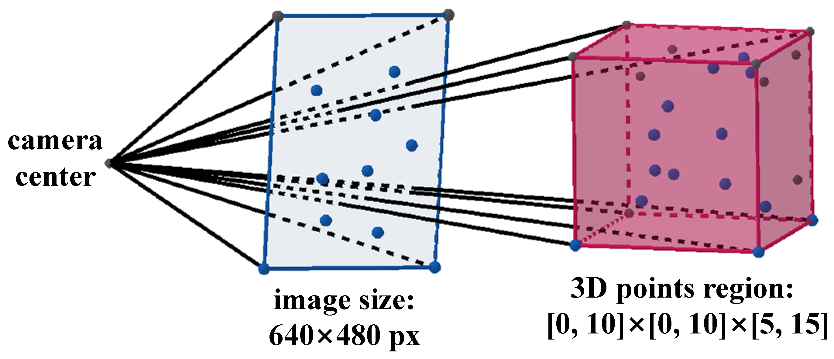
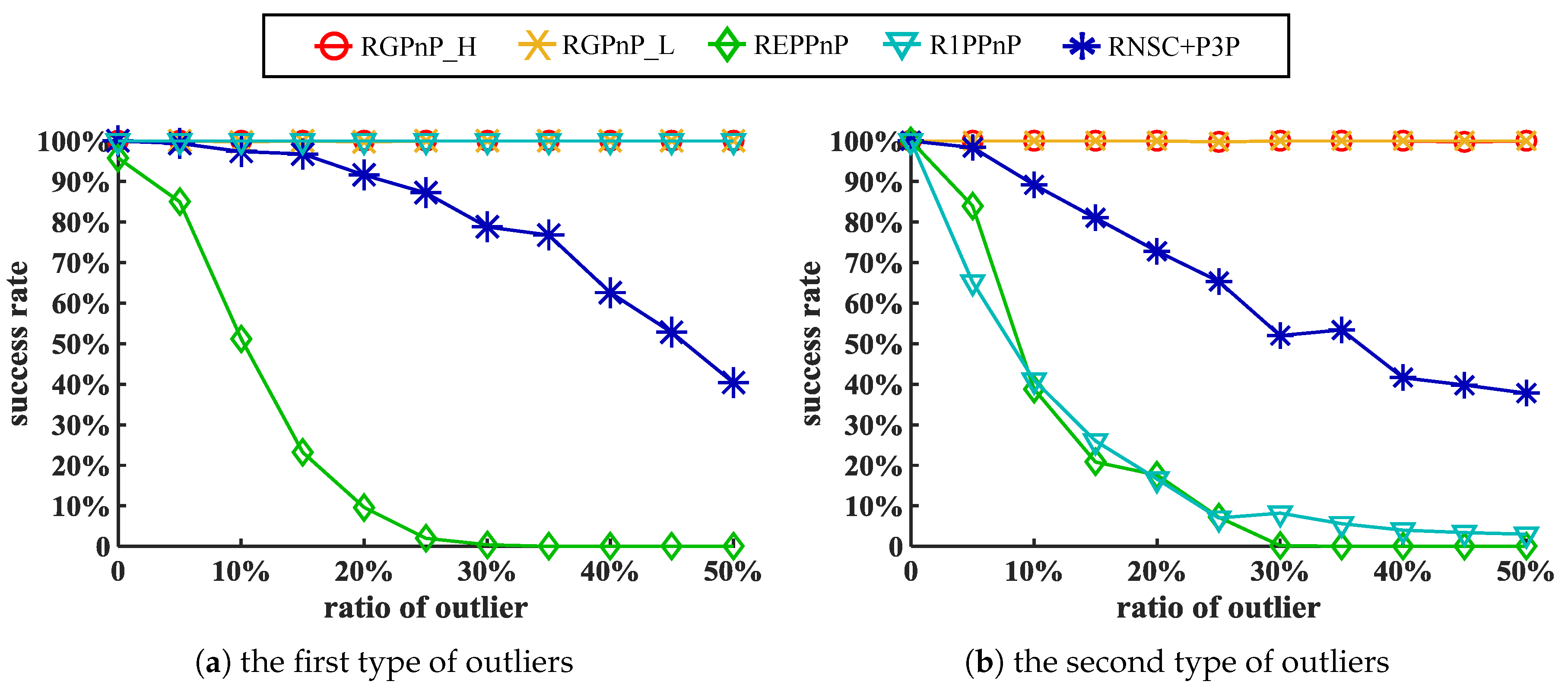
For synthetic experiments, we assumed a camera with an image size of $640\times 480$ and a focal length of 1000 pixels. We randomly generated 1000 3D points in a cubic region of $[0,10]\times [0,10]\times [5,15]$ and projected them onto the image to generate correct correspondences. Outliers were added to both the 3D points and 2D images to generate incorrect matches. Two different types of outliers were added, as follows: (1) Uniformly distributed 3D points were generated in the same cube as the data points ($[0,10]\times [0,10]\times [5,15]$), and each of them was assigned a correspondence to a randomly generated 2D points in the image. (2) Uniformly distributed 3D points were generated in a cubic region of $[0,1]\times [0,1]\times [0,1]$, different from the region of the data points, and each of them was assigned a correspondence to a randomly generated point in the image. The outlier ratio is defined as $r_{outlier}=\frac{N_{outlier}}{N_{outlier}+N_{inlier}}$. We performed experiments with different outlier ratios, and, for each ratio, 500 trials were run for each method. Figure 4 shows an illustration of the input in this subsection.

To evaluate the estimation accuracy, we computed the rotation error in degrees between the ground-truth rotation ${\mathbf{R}}_{true}$ and the estimated $\mathbf{R}$ as $e_{rot}=\angle ({\mathbf{R}}_{true},\mathbf{R})$ and the translation error between the ground-truth translation ${\mathbf{t}}_{true}$ and the estimated $\mathbf{t}$ as $e_{trans}=\frac{\parallel {\mathbf{t}}_{true}-\mathbf{t}\parallel }{\parallel {\mathbf{t}}_{true}\parallel }\times 100\%$. We report the success rate, defined as the fraction of trials in which the correct pose was found, where an estimation was considered successful when $e_{rot}$ was less than 0.1 radius and $e_{trans}$ was less than 0.2. The success rates for 500 trials of each method for both types of outliers are plotted in Figure 5.

As illustrated in Figure 5, our methods performed well in all trials with both types of outliers, while R1PPnP [11] handled the first type of outliers well but failed on the second type. The RANSAC-based method found the correct pose in most trials with a small outlier ratio but failed in most trials when the outlier ratio was large. REPPnP’s [29] performance was unsatisfactory for both types of outliers.

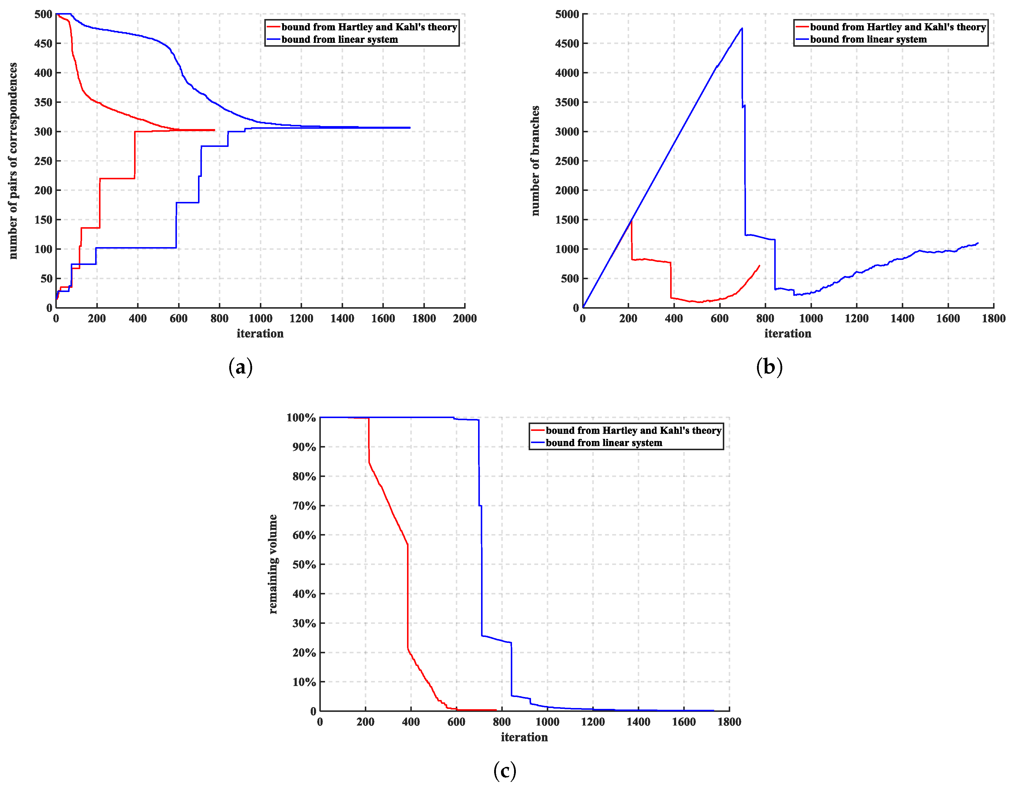
Global optimality. To demonstrate the global optimality of the proposed methods when solving the subprobelms, we ran a trial with 25% outliers of the first type. We present the evolution of the upper and lower bounds, the number of branches, and the remaining volume of rotation search for each of our methods in Figure 6. The upper and lower bounds converged after 775 iterations and 1731 iterations for RGPnP_H and RGPnP_L, respectively, indicating that the bounds derived from Hartley and Kahl’s theory are tighter than those derived from the linear system formulation.

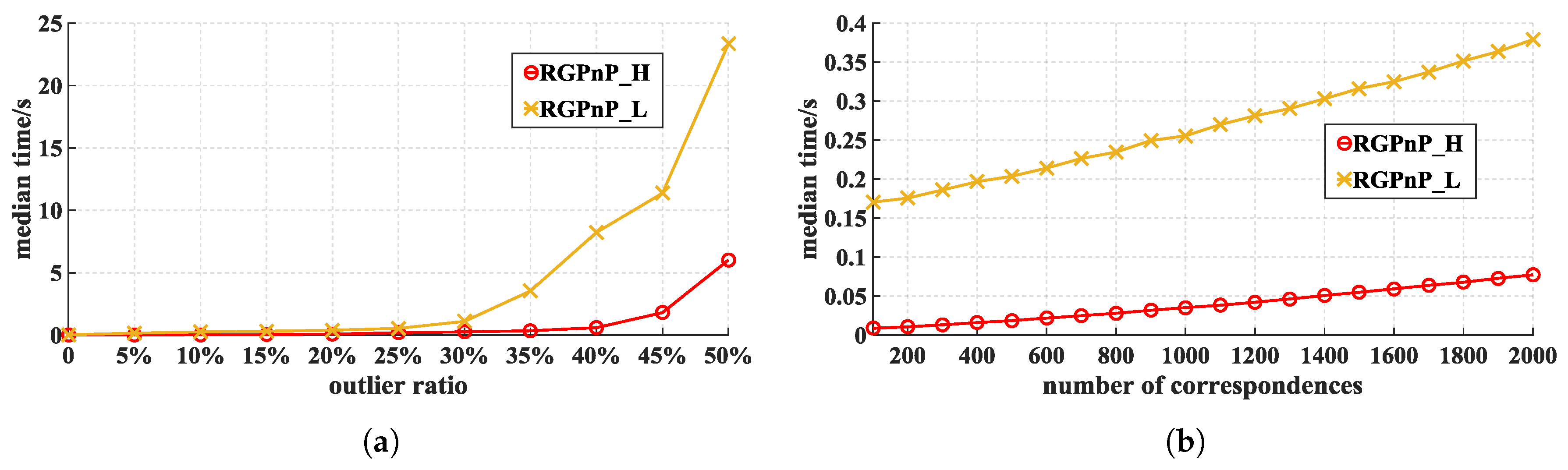
Complexity and scalability. In this section, we study the run time of the proposed method with respect to different outlier ratios and different numbers of correspondences. In the first experiment, there were 1000 correspondences in total, and we ran the two versions of the methods 500 times under different outlier ratios with outliers of the first type. The median run time among the 500 trials is shown in Figure 7a. RGPnP_H is faster than RGPnP_L, and the median run time of RGPnP_H is less than 1 s when the outlier ratio is no greater than 40%. Then, we experimentally investigated the scalability of the two methods. We ran each of the two methods 500 times with different numbers of correspondences and 10% outliers of the first type, and the results are presented in Figure 7b. Again, RGPnP_H is faster than RGPnP_L, and the run times of both methods increase approximately linearly with respect to the number of correspondences. Even with 2000 correspondences, the median run time of RGPnP_H is still less than 0.1 s. However, the run times are exponential in the outlier ratio, reflecting the hardness of the robust estimation problem.

4.2. Experiments with Real-World Data

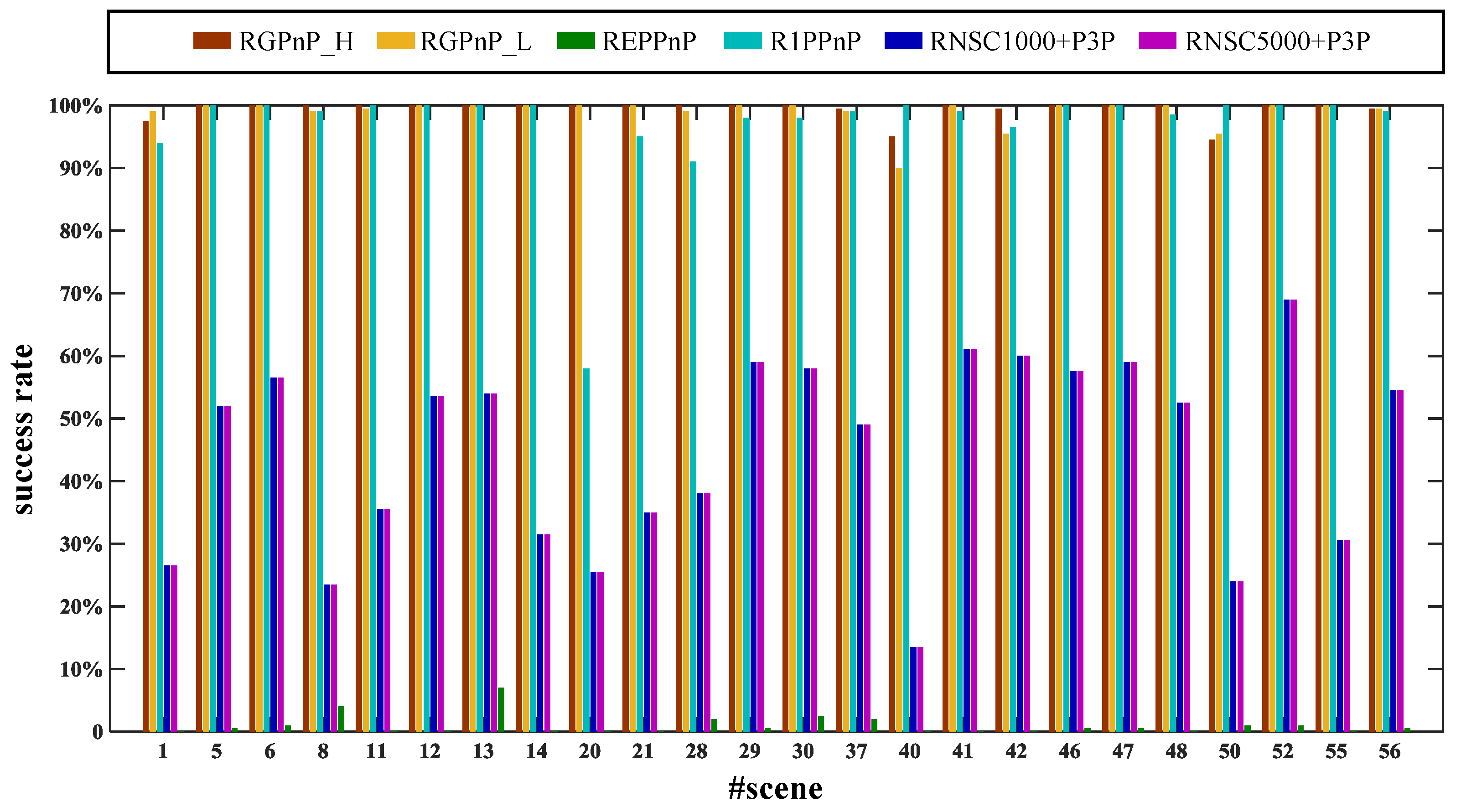
This section reports an evaluation conducted on the DTU Robot Image Data Sets [42]. The data consist of images of 60 scenes of different kinds of objects and materials, each of which was captured from 119 camera positions under 19 illumination situations. The 3D point clouds were obtained by means of structured light scanning. The calibration information is provided and the resolution of the images is $1600\times 1200$. For the experiment reported in this paper, 24 scenes were used. For each of these 24 scenes, we selected 20 camera positions and 10 illumination situations for each position, which resulted in a total of $24\times 20\times 10=4800$ 2D images. For each combination of scene and illumination situation, Image No. 25 was used as the reference image, and we matched SURF features between the reference image and the images from each of the 20 camera positions considered in this experiment to create the correspondences between each feature point in the reference image and points in the other images. Then, we reprojected the related 3D point cloud onto the plane of the reference image to find the correspondences between the 3D points and the 2D SURF feature points in the reference image. In this way, we indirectly created 2D–3D correspondences for each of the 4800 2D images used in this experiment. The number of correspondences for each image ranged from 49 to 220. Note that the correspondences created in this way contained both outliers and noise and that the outlier ratio varied with scenes, camera positions, and illumination situations.

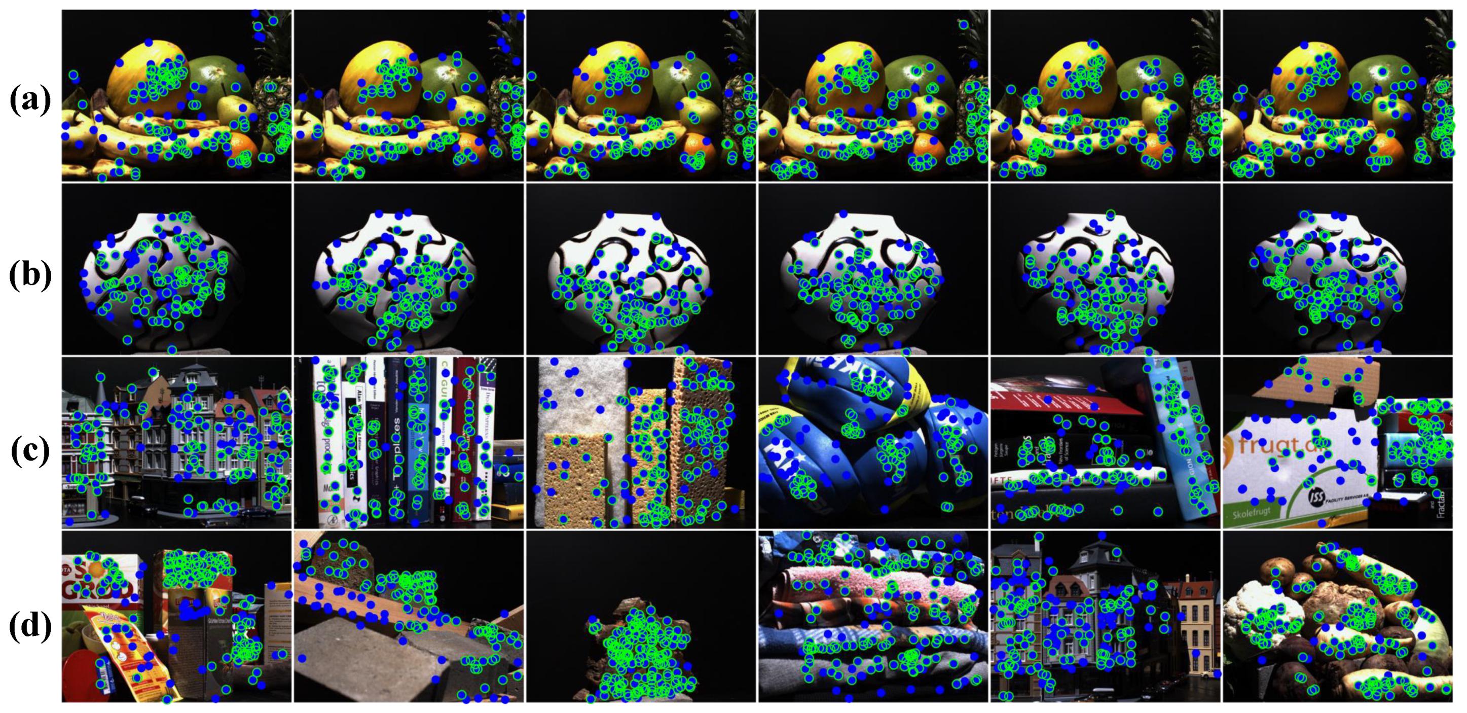
Then, we executed the five methods considered for comparison on all 4800 sets of 2D–3D correspondences and computed the estimation accuracy and the success rate as described in Section 4.1. The results are presented in Figure 8 and Figure 9. Both versions of the proposed method achieved a 100% success rate for almost all scenes, camera positions, and illumination situations. R1PPnP [11] achieved results similar to those of our methods, while the other compared methods failed in most trials. These results indicate that our methods produce the optimal solution and address outliers well. Figure 9 shows several examples of the real-world image data: after recovering the camera pose, we reprojected the 3D inliers onto the image plane with an inlier threshold of 10 pixels.

5. Discussion and Conclusions

In this paper, we propose a novel method of solving the absolute pose estimation problem. Our method was robust to outliers in the 2D–3D correspondences, and it solved the decoupled subproblems in a globally optimal way, which means that our method was able to produce guaranteed best solutions to the subproblems. Specifically, we reduced the dimensionality of the original problem from six to three, which made the BnB-based optimization process much faster. The 0.5 n-subset could be used as the input when the outlier ratio is low; however, if the outlier ratio is high, which will greatly increase the run time, we recommend the common trick of applying a heuristic outlier removal method to significantly reduce the outlier ratio before using our method. For our BnB algorithm solving the rotation search, we propose to use two upper bounds: the first one was derived from Hartley and Kahl’s rotation search theory and was more efficient for our problem, whereas the other was an original contribution that was more general and could be extended for application to other problems.

Limitations and improvements. Due to the decoupling scheme using the proposed pairwise constraints, our method achieved high efficiency yet sacrificed the joint global optimality for the original problem. As illustrated in Figure 7a, high outlier ratio always resulted in relatively long runtime for our method. The future improvements will mainly focus on implementation of efficient algorithm dealing with high outlier ratio scenario.

References

- Campbell, D.J.; Petersson, L.; Kneip, L.; Li, H. Globally-Optimal Inlier Set Maximisation for Camera Pose and Correspondence Estimation. IEEE Trans. Pattern Anal. Mach. Intell. 2018. [Google Scholar] [CrossRef] [PubMed]
- Grigorescu, S.M.; Macesanu, G.; Cocias, T.T.; Puiu, D.; Moldoveanu, F. Robust Camera Pose and Scene Structure Analysis for Service Robotics. Robot. Auton. Syst. 2011, 59, 899–909. [Google Scholar] [CrossRef]
- Putra, E.Y.; Wahyudi, A.K.; Dumingan, C. A proposed combination of photogrammetry, Augmented Reality and Virtual Reality Headset for heritage visualisation. In Proceedings of the 2016 International Conference on Informatics and Computing (ICIC), Mataram, Indonesia, 28–29 October 2016; pp. 43–48. [Google Scholar]
- Autran, C.; Guéna, F. 3D reconstruction of a disappeared museum. In Proceedings of the 2014 International Conference on Virtual Systems Multimedia (VSMM), Hong Kong, China, 9–12 December 2014; pp. 6–11. [Google Scholar]
- Lepetit, V.; Moreno-Noguer, F.; Fua, P. EPnP: An Accurate O(n) Solution to the PnP Problem. Int. J. Comput. Vis. 2009, 81, 155–166. [Google Scholar] [CrossRef] [Green Version]
- Taira, H.; Okutomi, M.; Sattler, T.; Cimpoi, M.; Pollefeys, M.; Sivic, J.; Pajdla, T.; Torii, A. InLoc: Indoor Visual Localization with Dense Matching and View Synthesis. In Proceedings of the IEEE Conference on Computer Vision and Pattern Recognition (CVPR), Salt Lake City, UT, USA, 18–22 June 2018; pp. 7199–7209. [Google Scholar]
- Sattler, T.; Leibe, B.; Kobbelt, L. Efficient and Effective Prioritized Matching for Large-Scale Image-Based Localization. IEEE Trans. Pattern Anal. Mach. Intell. 2017, 39, 1744–1756. [Google Scholar] [CrossRef] [PubMed]
- Guidi, G.; Beraldin, J.; Atzeni, C. High-accuracy 3D modeling of cultural heritage: the digitizing of Donatello’s “Maddalena”. IEEE Trans. Image Process. 2004, 13, 370–380. [Google Scholar] [CrossRef] [PubMed]
- Hess, M.; Petrovic, V.; Meyer, D.; Rissolo, D.; Kuester, F. Fusion of multimodal three-dimensional data for comprehensive digital documentation of cultural heritage sites. In Proceedings of the 2015 Digital Heritage, Granada, Spain, 28 September–2 October 2015; Volume 2, pp. 595–602. [Google Scholar] [CrossRef]
- Marchand, E.; Uchiyama, H.; Spindler, F. Pose Estimation for Augmented Reality: A Hands-On Survey. IEEE Trans. Vis. Comput. Graph. 2016, 22, 2633–2651. [Google Scholar] [CrossRef] [PubMed] [Green Version]
- Zhou, H.; Zhang, T.; Jayender, J. Re-weighting and 1-Point RANSAC-Base PnP Solution to Handle Outliers. IEEE Trans. Pattern Anal. Mach. Intell. 2018, 41, 3022–3033. [Google Scholar] [CrossRef] [PubMed]
- Svarm, L.; Enqvist, O.; Kahl, F.; Oskarsson, M. City-Scale Localization for Cameras with Known Vertical Direction. IEEE Trans. Pattern Anal. Mach. Intell. 2017, 39, 1455–1461. [Google Scholar] [CrossRef] [PubMed]
- Enqvist, O.; Kahl, F. Robust Optimal Pose Estimation. In Proceedings of the 10th European Conference on Computer Vision (ECCV), Marseille, France, 12–18 October 2008; pp. 141–153. [Google Scholar]
- Enqvist, O.; Ask, E.; Kahl, F.; Astrom, K. Robust Fitting for Multiple View Geometry. In Proceedings of the 12th European Conference on Computer Vision (ECCV), Florence, Italy, 7–13 October 2012; pp. 738–751. [Google Scholar]
- Wilcox, R. Introduction to Robust Estimation and Hypothesis Testing, 3rd ed.; Elsevier: Amsterdam, The Netherlands, 1997. [Google Scholar]
- Speciale, P.; Paudel, D.P.; Oswald, M.R.; Kroeger, T.; Gool, L.V.; Pollefeys, M. Consensus Maximization with Linear Matrix Inequality Constraints. In Proceedings of the 2017 IEEE Conference on Computer Vision and Pattern Recognition (CVPR), Honolulu, Hi, USA, 21–26 July 2017; pp. 5048–5056. [Google Scholar]
- Chin, T.; Suter, D.; Medioni, G.; Dickinson, S. The Maximum Consensus Problem: Recent Algorithmic Advances; Morgan & Claypool Publishers: San Rafael, CA, USA, 2017. [Google Scholar]
- Cai, Z.; Chin, T.J.; Le, H.; Suter, D. Deterministic Consensus Maximization with Biconvex Programming. In Proceedings of the European Conference on Computer Vision (ECCV), Munich, Germany, 8–14 September 2018; pp. 685–700. [Google Scholar]
- Chin, T.J.; Cai, Z.; Neumann, F. Robust fitting in computer vision: Easy or hard? In Proceedings of the European Conference on Computer Vision (ECCV), Munich, Germany, 8–14 September 2018; pp. 701–716. [Google Scholar]
- Enqvist, O.; Ask, E.; Kahl, F.; Astrom, K. Tractable Algorithms for Robust Model Estimation. Int. J. Comput. Vis. 2015, 112, 115–129. [Google Scholar] [CrossRef]
- Erickson, J.; Har-Peled, S.; Mount, D.M. On the Least Median Square Problem. Discret. Comput. Geom. 2006, 36, 593–607. [Google Scholar] [CrossRef] [Green Version]
- Bold, S.; Vandenberghe, L. Convex Optimization; Cambridge University Press: Cambridge, UK, 2004. [Google Scholar]
- Hartley, R.; Trumpf, J.; Dai, Y.; Li, H. Rotation Averaging. Int. J. Comput. Vis. 2013, 103, 267–305. [Google Scholar] [CrossRef]
- Zheng, Y.; Kuang, Y.; Sugimoto, S.; Åström, K.; Okutomi, M. Revisiting the PnP Problem: A Fast, General and Optimal Solution. In Proceedings of the 2013 IEEE International Conference on Computer Vision (ICCV), Sydney, NSW, Australia, 1–8 December 2013; pp. 2344–2351. [Google Scholar]
- Kneip, L.; Li, H.; Seo, Y. UPnP: An Optimal O(n) Solution to the Absolute Pose Problem with Universal Applicability. In Proceedings of the 13th European Conference on Computer Vision (ECCV), Zurich, Switzerland, 6–12 September 2014; pp. 127–142. [Google Scholar]
- Fischler, M.A.; Bolles, R.C. Random Sample Consensus: A Paradigm for Model Fitting with Applications to Image Analysis and Automated Cartography. Commun. ACM 1981, 24, 381–395. [Google Scholar] [CrossRef]
- Raguram, R.; Chum, O.; Pollefeys, M.; Matas, J.; Frahm, J. USAC: A Universal Framework for Random Sample Consensus. IEEE Trans. Pattern Anal. Mach. Intell. 2013, 35, 2022–2038. [Google Scholar] [CrossRef] [PubMed]
- Li, H. Consensus set maximization with guaranteed global optimality for robust geometry estimation. In Proceedings of the IEEE 12th International Conference on Computer Vision (ICCV), Kyoto, Japan, 29 September–2 October 2009; pp. 1074–1080. [Google Scholar]
- Ferraz, L.; Binefa, X.; Moreno-Noguer, F. Very Fast Solution to the PnP Problem with Algebraic Outlier Rejection. In Proceedings of the IEEE Conference on Computer Vision and Pattern Recognition (CVPR), Columbus, OH, USA, 24–27 June 2014; pp. 501–508. [Google Scholar]
- Camposeco, F.; Sattler, T.; Cohen, A.; Geiger, A.; Pollefeys, M. Toroidal Constraints for Two-Point Localization Under High Outlier Ratios. In Proceedings of the IEEE Conference on Computer Vision and Pattern Recognition (CVPR), Honolulu, HI, USA, 21–26 September 2017; pp. 4545–4553. [Google Scholar]
- Larsson, V.; Fredriksson, J.; Toft, C.; Kahl, F. Outlier Rejection for Absolute Pose Estimation with Known Orientation. In Proceedings of the British Machine Vision Conference, York, UK, 19–22 September 2016. [Google Scholar]
- Olsson, C.; Kahl, F.; Oskarsson, M. Branch-and-Bound Methods for Euclidean Registration Problems. IEEE Trans. Pattern Anal. Mach. Intell. 2009, 31, 783–794. [Google Scholar] [CrossRef] [PubMed]
- Briales, J.; Gonzalez-Jimenez, J. Convex Global 3D Registration with Lagrangian Duality. In Proceedings of the IEEE Conference on Computer Vision and Pattern Recognition (CVPR), Honolulu, HI, USA, 21–26 September 2017; pp. 4960–4969. [Google Scholar]
- Hartley, R.I.; Kahl, F. Global Optimization Through Rotation Space Search. Int. J. Comput. Vis. 2009, 82, 64–79. [Google Scholar] [CrossRef] [Green Version]
- Yang, J.; Li, H.; Campbell, D.; Jia, Y. Go-ICP: A Globally Optimal Solution to 3D ICP Point-Set Registration. IEEE Trans. Pattern Anal. Mach. Intell. (T-PAMI) 2016, 38, 2241–2254. [Google Scholar] [CrossRef] [PubMed] [Green Version]
- Li, H.; Hartley, R. The 3D–3D Registration Problem Revisited. In Proceedings of the IEEE 11th International Conference on Computer Vision, Rio de Janeiro, Brazil, 14–21 October 2007; pp. 1–8. [Google Scholar]
- Parra Bustos, A.; Chin, T.; Eriksson, A.; Li, H.; Suter, D. Fast Rotation Search with Stereographic Projections for 3D Registration. IEEE Trans. Pattern Anal. Mach. Intell. 2016, 38, 2227–2240. [Google Scholar] [CrossRef] [PubMed] [Green Version]
- Straub, J.; Campbell, T.; How, J.P.; Fisher, J.W. Efficient Global Point Cloud Alignment Using Bayesian Nonparametric Mixtures. In Proceedings of the 2017 IEEE Conference on Computer Vision and Pattern Recognition (CVPR), Honolulu, HI, USA, 21–26 September 2017; pp. 2403–2412. [Google Scholar]
- Ke, T.; Roumeliotis, S.I. An Efficient Algebraic Solution to the Perspective-Three-Point Problem. In Proceedings of the IEEE Conference on Computer Vision and Pattern Recognition (CVPR), Honolulu, HI, USA, 21–26 September 2017; pp. 7225–7233. [Google Scholar]
- Chin, T.; Purkait, P.; Eriksson, A.; Suter, D. Efficient Globally Optimal Consensus Maximisation with Tree Search. IEEE Trans. Pattern Anal. Mach. Intell. 2017, 39, 758–772. [Google Scholar] [CrossRef] [PubMed]
- Huynh, D.Q. Metrics for 3D Rotations: Comparison and Analysis. J. Math. Imaging Vis. 2009, 35, 155–164. [Google Scholar] [CrossRef]
- Aanæs, H.; Dahl, A.L.; Steenstrup Pedersen, K. Interesting Interest Points. Int. J. Comput. Vis. 2012, 97, 18–35. [Google Scholar] [CrossRef]
Figure 1.
Geometric relations and pairwise constraints between a pair of 3D points (blue) and their corresponding 2D points (red).
Figure 2.
Example of subset construction. There are points in 2D. If each point is used once, then we get three pairs of points as 0.5 n, which is randomly connected in our method. We can gradually increase the number of point-pairs until all point-pairs are used as 0.5 .
Figure 3.
Geometric interpretation. (a) The geometric interpretation of the first bound: under the action of all possible rotations within a cube in the angle-axis representation, a unit vector may lie only on a spherical patch on the 3D unit sphere. (b) The geometric interpretation of the second bound: a cube in the angle-axis representation can be mapped to a continuous domain in (for ease of visualization, it is plotted in a sphere).
Figure 4.
The illustration of the input in the experiments with synthetic data.
Figure 5.
Success rates for both types of outliers. An estimation was considered successful when was less than 0.1 radius and was less than 0.2.
Figure 6.
The optimality of RGPnP_H and RGPnP_L in rotation search. (a–c): The evolution of the upper and lower bounds, the number of branches, and the remaining volume.
Figure 7.
The complexity and scalability of RGPnP_H and RGPnP_L: (a) median run time versus the outlier ratio (with 1000 correspondences); and (b) median run time versus the number of correspondences (with 10% outliers).
Figure 8.
Success rates on the real-world data. An estimation was considered successful when was less than 0.1 radius and was less than 0.2.
Figure 9.
Examples of the real-world data. The blue spots are 2D feature points established by matching SURF features across different 2D images, and the green circles are the inliers reprojected using RGPnP. (a): Example images captured from different camera positions. (b): Example images captured under different illumination situations. (c,d): Example images of different scenes.
© 2019 by the authors. Licensee MDPI, Basel, Switzerland. This article is an open access article distributed under the terms and conditions of the Creative Commons Attribution (CC BY) license (http://creativecommons.org/licenses/by/4.0/).
Share and Cite
MDPI and ACS Style
Liu, Y.; Li, X.; Wang, M.; Knoll, A.; Chen, G.; Song, Z. A Novel Method for the Absolute Pose Problem with Pairwise Constraints. Remote Sens. 2019, 11, 3007. https://doi.org/10.3390/rs11243007
AMA Style
Liu Y, Li X, Wang M, Knoll A, Chen G, Song Z. A Novel Method for the Absolute Pose Problem with Pairwise Constraints. Remote Sensing. 2019; 11(24):3007. https://doi.org/10.3390/rs11243007
Chicago/Turabian StyleLiu, Yinlong, Xuechen Li, Manning Wang, Alois Knoll, Guang Chen, and Zhijian Song. 2019. "A Novel Method for the Absolute Pose Problem with Pairwise Constraints" Remote Sensing 11, no. 24: 3007. https://doi.org/10.3390/rs11243007
Note that from the first issue of 2016, this journal uses article numbers instead of page numbers. See further details here.