A Pragmatic Approach to the Design of Advanced Precision Terrain-Aided Navigation for UAVs and Its Verification

Abstract

Autonomous unmanned aerial vehicles (UAVs) require highly reliable navigation information. Generally, navigation systems with the inertial navigation system (INS) and global navigation satellite system (GNSS) have been widely used. However, the GNSS is vulnerable to jamming and spoofing. The terrain referenced navigation (TRN) technique can be used to solve this problem. In this study, to obtain reliable navigation information even if a GNSS is not available or the degree of terrain roughness is not determined, we propose a federated filter based INS/GNSS/TRN integrated navigation system. We also introduce a TRN system that combines batch processing and an auxiliary particle filter to ensure stable flight of UAVs even in a long-term GNSS-denied environment. As an altimeter sensor for the TRN system, an interferometric radar altimeter (IRA) is used to obtain reliable navigation accuracy in high altitude flight. In addition, a parallel computing technique with general purpose computing on graphics processing units (GPGPU) is applied to process a high resolution terrain database and a nonlinear filter in real-time on board. Finally, the performance of the proposed system is verified through software-in-the-loop (SIL) tests and captive flight tests in a GNSS unavailable environment.

1. Introduction

Recently, much research has been conducted on surveillance and reconnaissance technologies for autonomous unmanned aerial vehicles (UAVs). These UAVs require navigation information with utmost reliability and survivability. Traditionally, a navigation algorithm integrated with an inertial navigation system (INS) and a global navigation satellite system (GNSS) has been widely used [1,2]. The conventional INS has the advantage of providing continuous navigation information without external assistance. However, there is a disadvantage in that the navigation error increases due to sensor errors accumulated over time. In contrast, the GNSS cannot operate independently as it provides information with outside help and is vulnerable to hostile jamming and spoofing. To overcome such weaknesses, the vision-based navigation technique is commonly used for UAVs [3,4,5], but a problem with the camera adapting to the changing conditions of a real flight is not completely solved yet, so vision-based navigation is mainly used in drone systems that fly at low altitude for a relatively short time [6] and autonomous driving vehicles [7]. As another technique that can resolve the problems of GNSS, the terrain referenced navigation (TRN) can be used.

TRN is a navigation technology that estimates the aircraft’s precise position by comparing the altitude measured by an altimeter with the loaded digital elevation model (DEM) [8,9]. Existing TRN techniques use a radio altimeter to measure the distance between the ground level and the aircraft [10]. If a radio altimeter (RA) is used at a low altitude, a precise altitude measurement can be obtained because the radio wave reflection area is narrow, but if the altitude is higher than 800 m, the radio wave reflection area is wide, which increases the uncertainty of the reflected location of the wave and errors in the measured altitude increase. This makes the RA unsuitable for UAVs with reconnaissance missions at high altitudes. To overcome such deficiencies, Honeywell developed a TRN technique called precision terrain-aided navigation (PTAN) that is employed an interferometric radar altimeter (IRA) and was designed for the purpose of applying to the Tomahawk cruise missiles [11,12]. The IRA outputs the range and cross-track angle from aircraft to the nearest point on the zero Doppler line using two or more antennas [11]. As the output of the IRA can be converted to three-dimensional relative distances on an east-north-up (ENU) coordinate system, TRN based on an IRA can be used at high altitudes. We present a domestically developed IRA that can operate up to an altitude of 10 km.

On the other hand, to ensure the survivability and high reliability of UAVs, a TRN system should be able to obtain its current position even when a GNSS is unavailable for a long time and still guarantees a precise navigation performance similar to that of the INS/GNSS integrated navigation system. To ensure the survivability of UAVs when a GNSS is unavailable for a long time, a batch processing was used for the acquisition mode. The acquisition mode is a TRN technique that roughly estimates the current position when it has a large initial position error. To guarantee high reliability, a particle filter (PF) was used for the tracking mode and a high resolution DEM. The tracking mode is a TRN technique that preciously estimates the current position. To estimate precise location information from irregularly changing terrains, nonlinear estimation problems must be solved in real-time. As the extended Kalman filter (EKF)-based TRN may diverge due to local linearization [13], the PF was selected for the tracking mode. In addition, a parallel computing technology using general purpose computing on graphics processing units (GPGPU) was applied to implement the TRN algorithm based on PF and process the high-resolution DEM in real-time on board.

As mentioned above, unlike the GNSS, TRN is not affected by external interference, but its performance can be degraded in flat and repetitive terrain [14]. In order to mitigate individual deficiencies of TRN and GNSS and to ensure the high stability of UAVs, INS/GNSS/TRN integrated navigation is constantly being studied [15,16,17,18]. In [15,16], the INS/GNSS/TRN integrated navigation based on centralized filter was presented. However, it is very difficult to determine the logic of switching aiding sources or the conditions of determining priorities in a real flight environment. We designed a INS/GNSS/TRN-based on a federated filter that does not need to consider these problems. The federated filter is widely used in information fusion navigation systems because of its high computing efficiency [19]. All navigation sources are processed by local filters before they are merged into a master filter. The master filter of the INS/GNSS/TRN integrated navigation system uses the estimates and covariances of two local filters—INS/GNSS- and INS/TRN-aided filters. The local filters are designed with an EKF, which is a feedforward type of filter and is composed of the 18th state variables, and the INS/GNSS-aided navigation includes the barometer error compensation method.

Finally, before the proposed advanced precision terrain aided navigation system (AP-TAN) is applied to UAVs, it is necessary to complete a performance verification step on a real aircraft platform. Therefore, in this study, the captive flight tests were performed under various conditions to verify the proposed system. As it is expensive to carry out a captive flight test, various simulations and software-in-the-loop (SIL) experiments using the IRA, GNSS, Barometer simulators were performed in advance with the flight tests.

In Section 2, we introduce the design of the INS/GNSS/TRN integrated navigation algorithm based on the federated filter. First, we introduce the overall design of the proposed AP-TAN. Next, the master filter of the integrated navigation is described. In Section 3, we propose the design of a hybrid TRN based on the combination of batch processing and a PF using an IRA and a high-resolution DEM. First, the three-dimensional relative distance from the aircraft to a nearest point was derived from an IRA measurement. Next, the TRN algorithm based on batch processing for the acquisition mode and a PF for the tracking mode is explained. In Section 4, the simulation results are shown in various terrain conditions with the SIL experiments. Finally, we describe the captive flight tests that were conducted to analyze the navigation performance of the proposed system.

2. Design of the Proposed AP-TAN System

2.1. Overall Design of the AP-TAN System

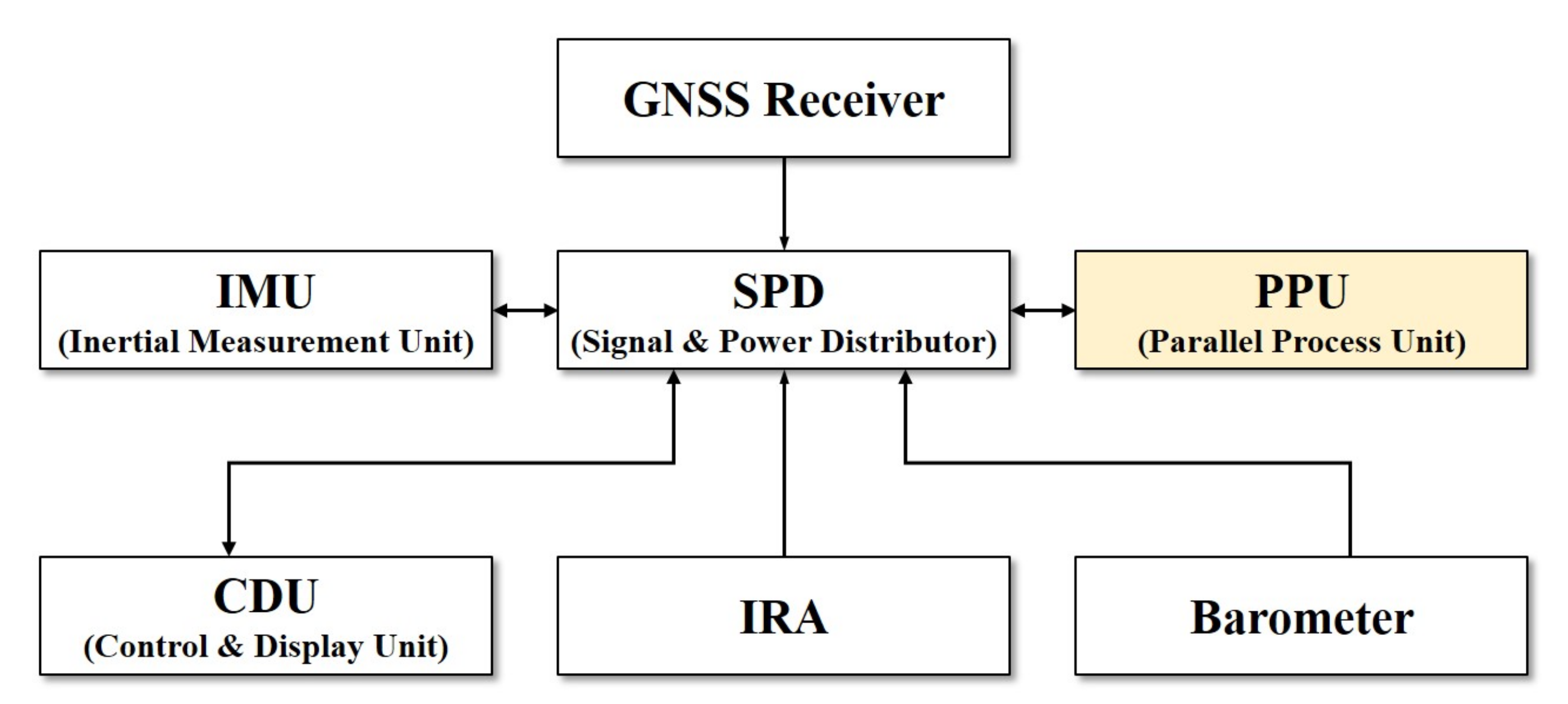
As shown in Figure 1, the proposed AP-TAN consists of the following.

• A inertial measurement unit (IMU) consists of three ring laser gyros (RLGs) and three silicon pendulum accelerometers to measure the motion of the vehicle without external helps.
• A parallel process unit (PPU) processes the outputs of a IMU and auxiliary sensors. It also performs navigation algorithms including pure navigation, INS/GNSS-aided navigation, TRN, INS/TRN-aided navigation, and INS/GNSS/TRN integrated navigation.
• A GNSS receiver provides the navigation information of the vehicle using GNSS outputs
• A barometer provide the altitude information of the vehicle by measuring the air pressure from the average sea level.
• A IRA provides 3D terrain elevation information for the nearest point.
• A control and display unit (CDU) gives control commands to the PPU and monitors the navigation results in real time.
• A signal and power distributor (SPD) delivers the commands from the CDU and the outputs of the auxiliary sensors to the PPU. It also delivers the navigation results from the PPU to the CDU. In addition, it provides adequate power for the entire system components.

In this study, we mainly deal with the software of the proposed AP-TAN. However, as pure navigation and GNSS navigation are already widely known, they are omitted. In this section, we introduce the INS/GNSS/TRN integrated navigation system.

2.2. Design of an INS/GNSS/TRN Integrated Navigation System

To achieve integrated navigation, an appropriate design of an information fusion filter is necessary, it can be divided into centralized and federated filters according to the method of processing measurements. The centralized filter is a method of selectively using the measurements of sensors in one filter, while the federated filter is composed of local filters using the measurements of each sensor and fuses the weighted estimates of local filters using their covariances [20,21]. With a centralized filter, an optimal solution can be found, but if a sensor fails, the performance degrades. Moreover, implementing the logic to properly select measurements in one filter is not easy. In addition, proper fusion of information from auxiliary sensors in one filter requires much experience. On the other hand, with a federated filter, only estimates and covariances are used, which reduces the number of variables passed to the master filter and reduces the burden of designing selective decision logic of measurements. Therefore, in this section, we describe our design of a federated filter-based INS/GNSS/TRN integrated navigation using INS/GNSS-aided navigation and INS/TRN-aided navigation filters as local filters. The local filters are designed with an EKF, which is an indirect feedforward type and composed of the 18th state variables. Along with two local filters, the INS/GNSS-aided navigation includes the barometer error compensation method.

2.2.1. Design of the Master Filter Based on the Federated Filter

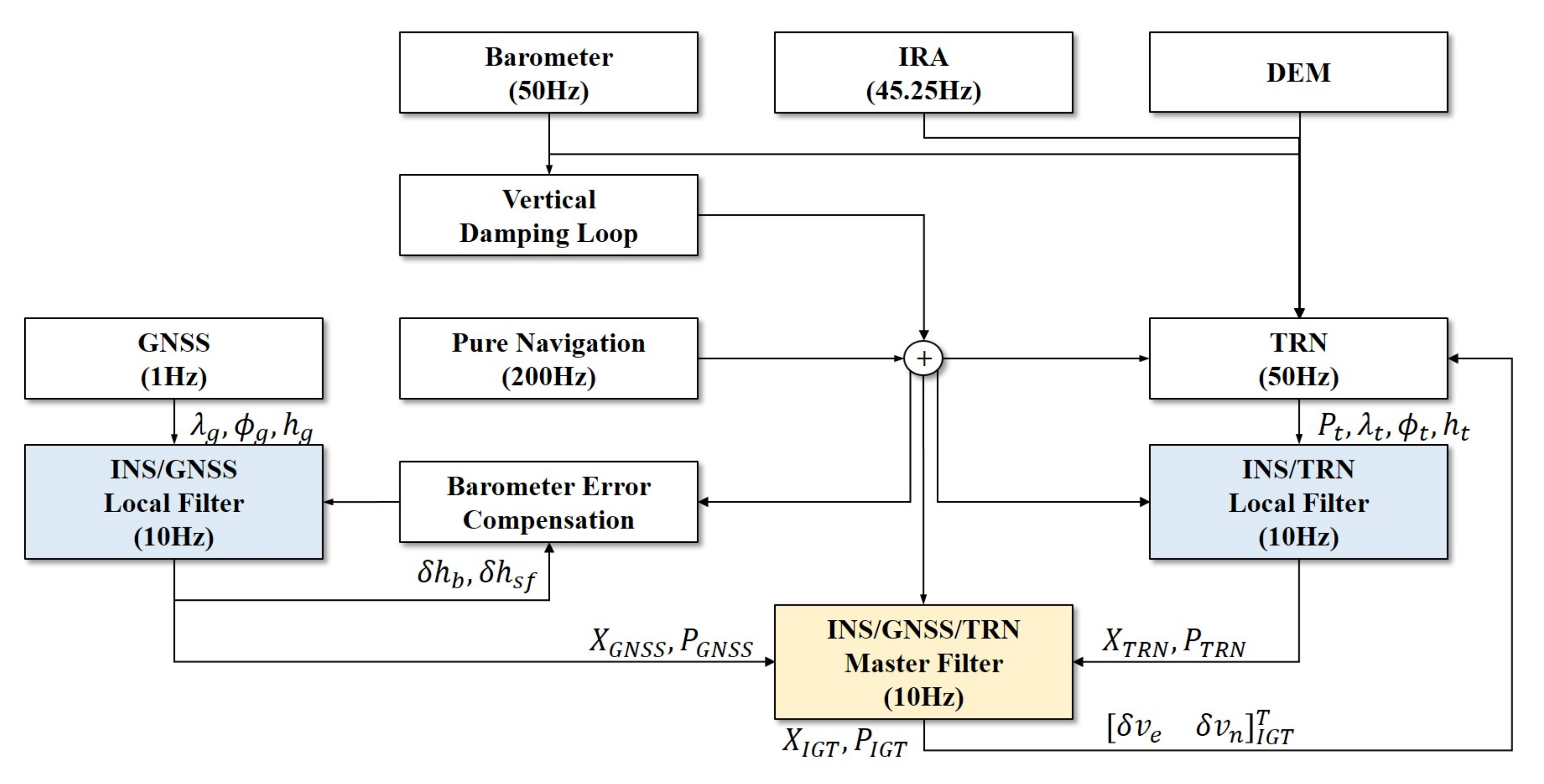
The federated filter consists of local filters and a master filter, and has a structure that obtains the master filter estimate by fusing the estimates of the local filters. This structure allows local filters to be designed independently to prevent cross contamination between them and to reduce the amount of computation as there is no need to calculate their mutual covariance [20]. In this system, we designed a federated filter-based integrated navigation system in the fault-tolerant (FT) mode that does not guarantee an optimal solution but is robust against sensor failure. Figure 2 shows a block diagram of the federated filter-based INS/GNSS/TRN integrated navigation with INS/GNSS-aided navigation and INS/TRN-aided navigation as local filters.

The pure navigation in Figure 2 is a navigation algorithm that calculates the position, velocity, and attitude using the outputs of the gyro and accelerometer. The position output of pure navigation is used in the time propagation of the TRN filter. In addition, the position, velocity, and attitude information of pure navigation is used to update the system matrix of the local filters. However, as the altitude error estimated by pure navigation increases exponentially with time, it is replaced by the output of the vertical damping loop with the barometer to obtain a stable vertical navigation performance. As shown in Figure 2, the local and master filters are updated at 10 Hz periods. In INS/GNSS-aided navigation, GNSS measurements are updated every 1 Hz, so the filter is designed to perform only the time propagation in the intervals between measurement updates. The longitude, latitude, and altitude estimates of GNSS, ${\lambda }_g$, ${\varphi }_g$, and $h_g$, are used as measurements for the INS/GNSS-aided navigation, and the diagonal elements of the measurement noise covariance matrix are set at fixed values. In this system, the IRA and barometer were used to obtain altimeter measurements to compare with the DEM altitude. As shown in Figure 2, the IRA measurement is updated at 45.25 Hz cycles, so it is synchronized by latching pure navigation results. When the measurement is not updated within the TRN filter period of 50 Hz, it is designed to perform only time propagation. As mentioned in the previous section, the TRN of this system used batch processing as an acquisition mode for estimating the approximate position when the initial position error was large, and an auxiliary particle filter (APF) as a tracking mode for estimating the precise position. INS/TRN aided navigation is designed to be performed only in the APF-based tracking mode. The INS/TRN-aided navigation uses the longitude, latitude, and altitude estimates of TRN ${\lambda }_t$, ${\varphi }_t$, and $h_t$ and their covariance matrix $P_t$ as the measurement and the measurement noise covariance matrix, respectively.

The INS/GNSS/TRN integrated navigation algorithm using INS/GNSS-aided navigation and INS/TRN aided navigation as local filters is as follows.

Case 1.

The state variables and covariances when GNSS is not available.

$$P_{IGT}\left(k\right)=P_{TRN}\left(k\right),X_{IGT}\left(k\right)=X_{TRN}\left(k\right)$$

(1)

Case 2.

The state variables and covariances when TRN is not available.

$$P_{IGT}\left(k\right)=P_{GNSS}\left(k\right),X_{IGT}\left(k\right)=X_{GNSS}\left(k\right)$$

(2)

Case 3.

The state variables and covariances when both GNSS and TRN are available.

$$P_{IGT}\left(k\right)={\left[{\left(P_{GNSS}\left(k\right)\right)}^{-1}+{\left(P_{TRN}\left(k\right)\right)}^{-1}\right]}^{-1}$$

(3)

$$X_{IGT}\left(k\right)=P_{IGT}\left(k\right)\left[P_{GNSS}{\left(k\right)}^{-1}{X}_{GNSS}\left(k\right)+P_{TRN}{\left(k\right)}^{-1}{X}_{TRN}\left(k\right)\right]$$

(4)

Case 4.

The state variables and covariance when both GNSS and TRN are not available.

$$X_{IGT}\left(k\right)=\left(I+A_{IGT}\Delta t\right)X_{IGT}(k-1)={\mathsf{\Phi }}_{IGT}{X}_{IGT}(k-1)$$

(5)

$$P_{IGT}\left(k\right)={\mathsf{\Phi }}_{IGT}{P}_{IGT}(k-1){\mathsf{\Phi }}_{IGT}^T+Q_{IGT}$$

(6)

Here, $X_{IGT}\left(k\right)$ and $P_{IGT}\left(k\right)$ are the estimated state variable vector and the estimated covariance matrix of the master filter, respectively. The estimated state variable vectors and estimated covariance matrices of the INS/GNSS and INS/TRN local filters are represented as $X_{GNSS}\left(k\right)$, $P_{GNSS}\left(k\right)$, $X_{TRN}\left(k\right)$, and $P_{TRN}\left(k\right)$, respectively, and $Q_{IGT}$ and $R_{IGT}$ represent the process noise covariance and measurement noise covariance of the master filter, respectively. $A_{IGT}$ and $\Delta t$ are the system matrix and filter update period, respectively. The first-order Taylor expansion of the system matrix, $A_{IGT}$, is computed for the discrete system matrix, ${\mathsf{\Phi }}_{IGT}$. The master filter and local filters use the 18th state variables composed of the errors of latitude, longitude, altitude, velocity and attitude, accelerometer bias, gyro bias, barometer error compensation acceleration, barometer bias, and barometer scale factor. If both TRN and GNSS are not available, as in Case 4, the master filter only performs time propagation in Equations (5) and (6). If there is any available local filter, the master filter performs not only the time propagation but also the appropriate measurement update for each case. The unavailability of GNSS and TRN in Cases 1 and 2 means that the system itself is inoperable. Case 3 applies when GNSS or TRN is temporarily unavailable.

2.2.2. Design of the Local Filters Based on the EKF

As mentioned in the previous section, the local filters of this system are composed of 18th state variables as follows.

$$X_{GNSSorTRN}={\left[\delta \lambda \delta \varphi \delta h\delta v_e\delta v_n\delta v_u\delta {\phi }_e\delta {\phi }_n\delta {\phi }_u\delta B_x^a\delta B_y^a\delta B_z^a\delta B_x^w\delta B_y^w\delta B_z^w\delta a\delta h_b\delta h_{sf}\right]}^T$$

(7)

Here, $\left[\delta \lambda \delta \varphi \delta h\right]$ is the error vector of longitude, latitude, and altitude, and $\left[\delta v_e\delta v_n\delta v_u\right]$ is the velocity error vector in the ENU coordinate system. $\left[\delta {\phi }_e\delta {\phi }_n\delta {\phi }_u\right]$ is the error vector of roll, pitch, and yaw; $\left[\delta B_x^a\delta B_y^a\delta B_z^a\right]$ and $\left[\delta B_x^w\delta B_y^w\delta B_z^w\right]$ are the accelerometer bias error and the gyro bias error vector in the body frame, respectively; and $\delta a$, $\delta h_b$, and $\delta h_{sf}$ denote the barometer error compensation acceleration, barometer bias, and barometer scale factor, respectively. The state variable configuration is identical to the two local filters and the master filter, but the barometer bias and scale factor error compensation is designed to be performed only in the local filter corresponding to the INS/GNSS-aided navigation. As mentioned in the previous section, APF-based TRN was designed to compensate for the vertical bias error in the IRA and barometer when the likelihood function is calculated. Therefore, if the barometer error is additionally compensated for the INS/TRN-aided navigation, the vertical bias error estimation of the APF, the filter used in the TRN tracking mode, may not normally be performed. Considering this point, our system is designed not to perform barometer error compensation in INS/TRN aided navigation.

First, we describe the barometer error estimation and compensation technique as well as the overall 18th local filter design. Barometer errors include bias errors modeled in the first-order Markov process, scale factor errors in the form of random constants, and white Gaussian noise. Applying the linear perturbation method to a system with a third-order vertical damping loop, the following vertical error model is derived [22].

$$\delta \dot{h}=\delta v_u-K_1\left(\delta h-\delta h_b-h\delta h_{sf}\right)$$

(8)

$$\delta {\dot{v}}_u=\delta A_z-K_2\left(\delta h-\delta h_b-h\delta h_{sf}\right)-\delta a+2{\omega }_s^2\delta h$$

(9)

$$\delta \dot{a}=K_3\left(\delta h-\delta h_b-h\delta h_{sf}\right)$$

(10)

$$\delta {\dot{h}}_b=-\frac{1}{\tau }\delta h_b+{\omega }_B$$

(11)

$$\delta {\dot{h}}_{sf}=0$$

(12)

Here, ${\omega }_B$ is the white noise of the barometer. If the 2nd and 1st gains and the bias of the damping loop characteristic equation are $K_1$, $K_2$, and $K_3$, respectively, it can be calculated as follows,

$$K_1=\frac{3}{\tau },K_2=2{\omega }_s^2+\frac{3}{{\tau }^2},K_3=\frac{1}{{\tau }^3}$$

(13)

Here, $\tau$ is the time constant of the system and ${\omega }_s$ is the Sculler frequency. The above barometer bias and scale factor error estimation and compensation are applied only to INS/GNSS-aided navigation. However, in the initialization step of INS/TRN-aided navigation, the barometer bias and scale factor error estimated by the INS/GNSS-aided navigation are taken once. Two local filters were designed with an indirect feedforward EKF using the system matrix $A\left(k\right)$ and the measurement matrix H are described in [23].

Unlike INS/GNSS-aided navigation, we designed semi-tightly coupled structure when combining TRN and INS. Therefore, an aircraft movement input vector is required for the prior pdf for time propagation of APF-based TRN. In this study, we used the INS position increments and the integrated navigation velocity increments. redThe design of the filter has the excellent initial transient characteristic and overall performance, and is applied as shown in Figure 2.

3. Hybrid TRN Algorithm Based on an Interferometric Radar Altimeter

The three key parameters that determine the performance of TRN are a precision altimeter, an optimal TRN algorithm, and a high-resolution terrain database. In addition to developing a precision altimeter, it is also important to design an appropriate error compensation method and a measurement validity check logic for an altimeter. Next, to enhance the performance of TRN even when GNSS is unavailable for a long time, an optimal TRN algorithm should be designed. The TRN algorithm should include the validity check logic of the terrain roughness and uniqueness to prevent performance degradation on flat or repetitive terrain. Finally, we need to build a high-resolution DEM and develop appropriate matching technology with altimeter measurements for precise TRN. Moreover, the TRN algorithm with the high-resolution DEM must be capable of real-time processing on board. Considering these requirements, we propose the hybrid TRN algorithm that uses batch processing for the acquisition mode and a PF for the tracking mode. We used an IRA as the altimeter and a multi-resolution terrain database with a combination of a 3 m DEM level 4 and a 10 m resolution DEM level 3. To guarantee the real-time implementation on board, we used a parallel computing technology based on GPGPU in the proposed TRN system.

3.1. Error Compensation Method of IRA Measurements

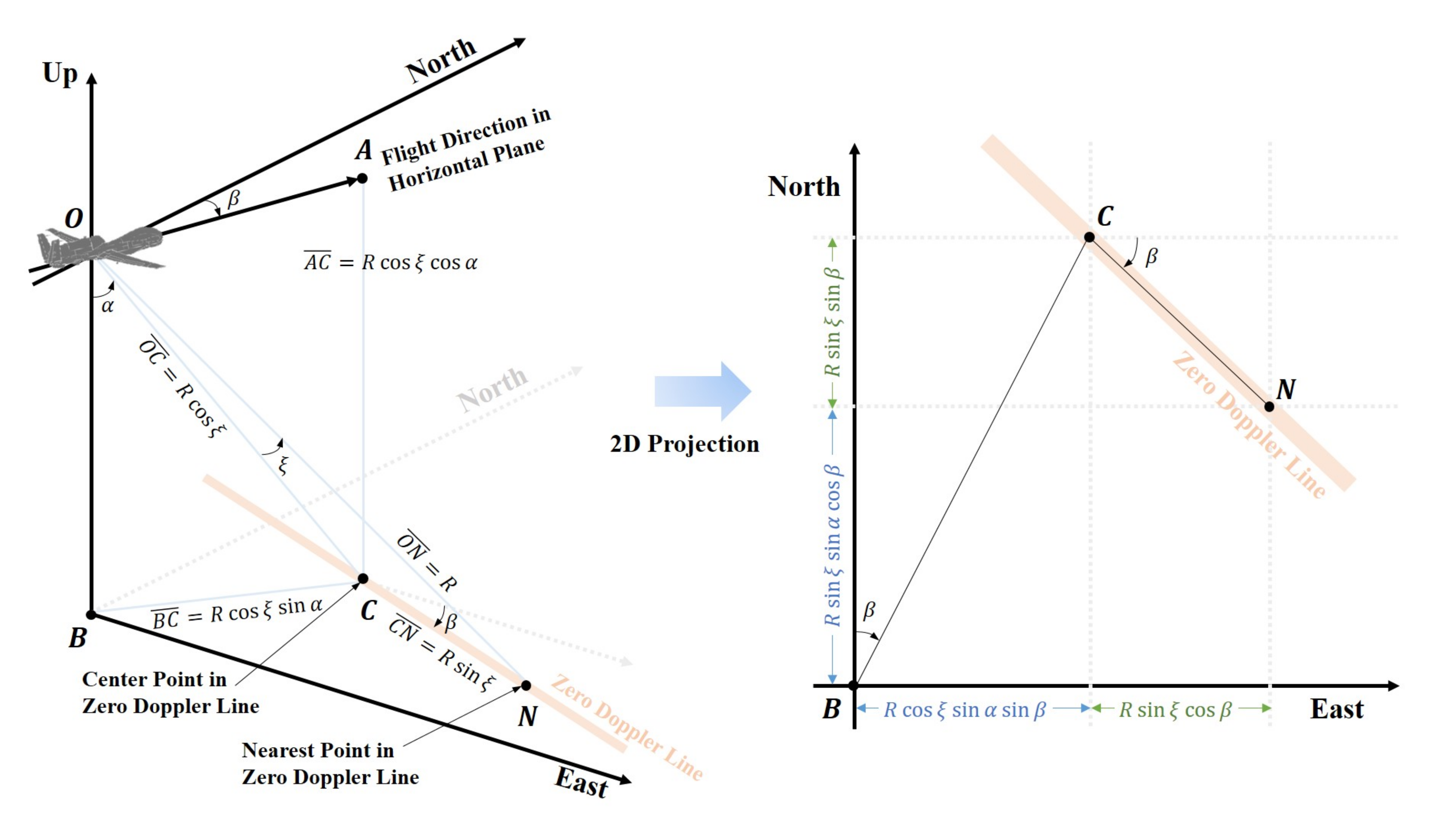
An IRA outputs not only the relative distance (slant range, R), but also the cross-track angle (look angle, $\theta$) from an aircraft to the nearest point on the zero Doppler line using the principle of interferometry [11]. The zero Doppler line is perpendicular to the velocity vector of the aircraft [11]. When the direction cosine matrix (DCM) required for converting IRA measurements to relative positions in the ENU coordinate system was calculated using Euler angles as shown in [24], there was performance degradation in a real flight environment [11]. This degradation is due to the angle of attack and the side slip angle caused by wind during flight. Therefore, in this study, to extract precision 3D position information, the effective look angle $\xi$ should be calculated with the IRA look angle $\theta$, and the virtual attitude calculated by the velocity of the aircraft, as shown in Figure 3 [25].

The relative position vector $x_{IRA,k}$ of the nearest point, the virtual azimuth angle $\beta$, the virtual pitch angle $\alpha$, and the effective look angle $\xi$ can be determined as follows.

$$x_{IRA,k}=\left[\begin{array}{c}\hfill p_{e,k}\\ \hfill p_{n,k}\\ \hfill p_{u,k}\end{array}\right]=\left[\begin{array}{c}\hfill \rho cos\xi sin\alpha sin\beta +\rho sin\xi cos\beta \\ \hfill \rho cos\xi sin\alpha cos\beta -\rho sin\xi sin\beta \\ -\rho cos\xi cos\alpha \end{array}\right]$$

(14)

$$\beta =\{\begin{array}{c}\hfill \frac{\pi }{2}-{tan}^{-1}\frac{V_n}{V_e},\left|\frac{V_e}{V_n}\right|>1\\ \hfill {tan}^{-1}\frac{V_e}{V_n},\left|\frac{V_e}{V_n}\right|\le 1\end{array}$$

(15)

$$\alpha ={tan}^{-1}\frac{V_u}{\sqrt{V_e^2+V_n^2}}$$

(16)

$$\xi ={sin}^{-1}\frac{sin\theta }{\sqrt{{\alpha }^2{sin}^2\left(\psi -\beta \right)+{cos}^2\left(\psi -\beta \right)}}-{tan}^{-1}\frac{-\alpha sin\left(\psi -\beta \right)}{cos\left(\psi -\beta \right)}$$

(17)

Here, $\psi$ is the yaw of the aircraft. A detailed derivation process is given in Section 2 in [25]. ${\left[V_e,V_n,V_u\right]}^T$ is the velocity of the aircraft in the ENU frame. Typically, ${\left[V_e,V_n\right]}^T$ is the estimates of the INS/GNSS/TRN integrated navigation and $V_u$ is the estimate of the barometer damping loop. This is because the upward velocity error estimated by the INS/GNSS/TRN integrated navigation increases exponentially when neither a GNSS nor TRN is available. This misleads the IRA measurements as unavailable, further degrading the integrated navigation performance. Therefore, in this study, we use an upward velocity estimate of the barometer damping loop that shows stable changes during flight.

3.2. Acquisition Mode Based on Batch Processing

TRN based on batch processing calculates the navigation solution by comparing the terrain elevation profile collected during a certain correction period with the reference matrix [26]. Here, the reference matrix refers to a matrix with the terrain elevations extracted from the DEM around the current position of the aircraft as elements. When the correction period of TRN is reached, the matching reference elevation set can be acquired by comparing the measured terrain elevation profile with the DEM reference matrix. In that case, the mean absolute difference (MAD) and the mean square difference reference matrix (MSD) are defined as follows [11].

$$MA{D}_{i,j}=\frac{1}{N}\sum _{k=1}^N\left|\left(h_{baro,k}-p_{u,k}\right)-h_{DB}\left(\widehat{\lambda }+i\Delta \lambda +p_{lon,k},\widehat{\phi }+j\Delta \phi +p_{lat,k}\right)\right|$$

(18)

$$MS{D}_{i,j}=\frac{1}{N}\sum _{k=1}^N{\left[\left(h_{baro,k}-p_{u,k}\right)-h_{DB}\left(\widehat{\lambda }+i\Delta \lambda +p_{lon,k},\widehat{\phi }+j\Delta \phi +p_{lat,k}\right)\right]}^2$$

(19)

Here, N is the number of samples in the measured terrain elevation profile. $h_{DB}$ is the terrain elevation value of the DEM. $\widehat{\lambda }$ and $\widehat{\phi }$ are the longitude and latitude, respectively, estimated by INS. $\Delta \lambda$ and $\Delta \phi$ are the longitudinal and latitudinal cell size of the reference matrix, respectively. i and j are the column and row index for the reference matrix, respectively. $p_{lon,k}$ and $p_{lat,k}$ are the east and north direction relative positions to the nearest point, respectively. These are calculated using Equation (14) as follows.

$$p_{lon,k}=\frac{p_{e,k}}{R_{ew}cos\widehat{\phi }},p_{lat,k}=\frac{p_{n,k}}{R_{ns}}$$

(20)

Here, $R_{ew}$ and $R_{ns}$ represent the radius of the curvature of the Earth ellipsoid in the east–west and north–south directions, respectively. As shown in [26], the TRN output based on batch processing was determined as the position with the minimum MAD or MSD value in the reference matrix. Therefore, in this study, we designed the following conditions where the acquisition mode is converted to a tracking mode.

$$\sqrt{MS{D}_{min}}<{\sigma }_{MSD1},\sqrt{MS{D}_{sec,min}}-\sqrt{MS{D}_{min}}>{\sigma }_{MSD2}$$

(21)

$$\left|MS{D}_{min}-MA{D}_{min}\right|\le {\sigma }_{MSD3}$$

(22)

Here, $MS{D}_{min}$ and $MS{D}_{sec,min}$ represent the minimum and the second minimum values of the MSD, respectively. $MA{D}_{min}$ represents the minimum value of the MAD. In this study, ${\sigma }_{MSD1}$, ${\sigma }_{MSD2}$, and ${\sigma }_{MSD3}$ are the thresholds for the conditions, respectively. Moreover, we designed to update the correction period when a certain number of measurements are collected without fixing the period. In other words, the acquisition is completed quickly in rough and unique terrain and the acquisition is performed for a long time in a flat and repetitive area. This batch processing has the disadvantage of having a long update period, but the calculation is relatively simple, which is suitable for the purpose of finding a coarse position in a wide search area. Therefore, in this study, we applied batch processing for the acquisition mode to estimate the current position roughly when the initial position error is large. The size of the reference matrix was set to $1001\times 1001$ so that it can be searched for even when there is an initial position error of up to 2.5 km.

3.3. Tracking Mode Based on a Particle Filter

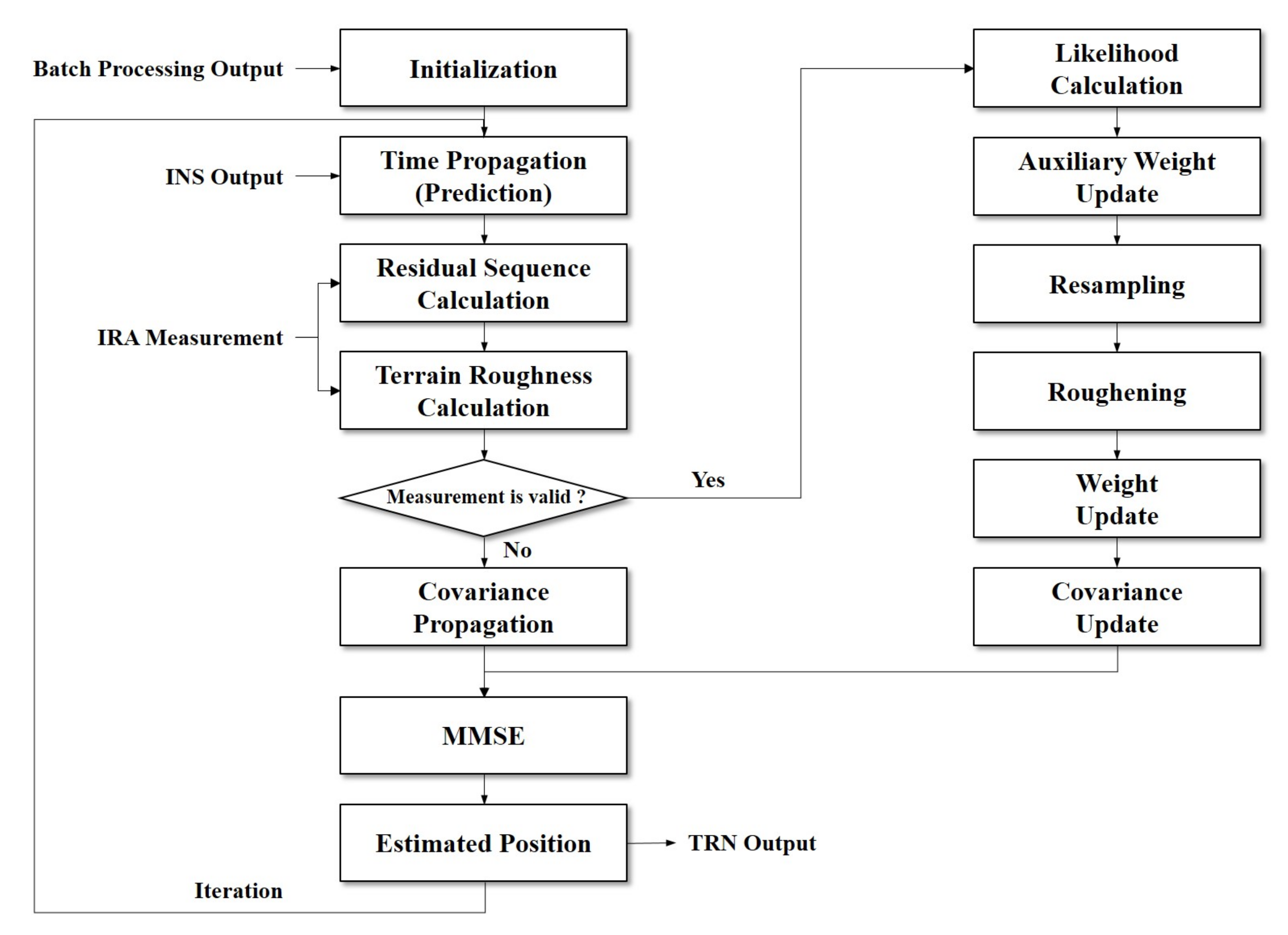
To estimate the precise position by TRN, nonlinear estimation problems have to be solved in real-time [14]. As the EKF locally linearizes the highly nonlinear characteristics of terrains, the EKF-based TRN algorithm can diverge or degrade performance. Recently, to solve this problem, PF-based TRN techniques have been actively studied [27,28,29,30]. Among the various PFs, the auxiliary particle filter (APF) was applied for the tracking mode of TRN in this study. The APF was first introduced by Pitt and Shephard in [28] to improve deficiencies in the general sequential importance resampling (SIR) algorithm. In this study, we used the APF, which is easy to implement and shows stable performance in IRA-based TRN. The APF-based TRN algorithm execution flowchart is shown in Figure 4.

Assume the state vector of the APF is $x_{k|k}={\left[{\delta x}_e,{\delta x}_n,{\delta x}_u\right]}^T$. It is a state vector composed of the position errors on the ENU coordinate at the time step k. First, the state vector and the weight of the particles must be initialized using the estimates by the batch processing. Next, the time propagation of the states and weights is calculated as follows.

$$x_{k|k-1}^{\left[i\right]}\approx q\left(x_{k|k-1}^{\left[i\right]}|x_{k-1|k-1}^{\left[i\right]},y_{k-1}\right)$$

(23)

$$w_{k|k-1}^{\left[i\right]}\approx \frac{p\left(y_k|x_{k|k-1}^{\left[i\right]}\right)p\left(x_{k|k-1}^{\left[i\right]}|x_{k-1|k-1}^{\left[i\right]}\right)}{q\left(x_{k|k-1}^{\left[i\right]}|x_{k-1|k-1}^{\left[i\right]},y_k\right)}{w}_{k-1|k-1}^{\left[i\right]}$$

(24)

$$p\left(x_{k|k-1}^{\left[i\right]}|x_{k-1|k-1}^{\left[i\right]}\right)=P_{{\omega }_k}\left(x_{k|k-1}^{\left[i\right]}-x_{k-1|k-1}-u_k\right)$$

(25)

Here, $x_{k|k-1}^{\left[i\right]}$ and $w_{k|k-1}^{\left[i\right]}$ are the state vector and the weight of the i-th particle in the prediction step, respectively. $x_{k-1|k-1}^{\left[i\right]}$ and $w_{k-1|k-1}^{\left[i\right]}$ are the values of the i-th particle in the previous update step. The current value of the state vector is determined by the previous value using a Markov process. $y_{k-1}$ is the terrain height calculated by the difference between the measurements of the IRA and the barometer in the previous step. The transition pdf, $p\left(x_{k|k-1}^{\left[i\right]}|x_{k-1|k-1}^{\left[i\right]}\right)$ is obtained via the Chapman–Kolmogorov equation [14]. ${\omega }_k$ is the white system process noise that meets $E\left({\omega }_k\right)=0$ and $E\left({\omega }_k{{\omega }_k}^T\right)=Q_c△t$. Here, $Q_c$ is the system process noise covariance in the PF, which was set to ${\left[0.04,0.04,0.04\right]}^T$, and $△t$ is the execution period, which was set to $0.02$ in this study. $P_{{\omega }_k}(x_{k|k-1}^{\left[i\right]}-x_{k-1|k-1}-u_k)$ is a Gaussian pdf with a standard deviation of ${\omega }_k$. $u_k$ is an aircraft movement input vector between $k-1$ and k time step. By using transition density as the proposal distribution, $q\left(x_{k|k-1}^{\left[i\right]}|x_{k-1|k-1}^{\left[i\right]},y_{k-1}\right)=p\left(x_{k|k-1}^{\left[i\right]}|x_{k-1|k-1}^{\left[i\right]}\right)$, the sequential weight update Equation (24) is simplified as follows.

$$w_{k|k-1}^{\left[i\right]}\approx p\left(y_k|x_{k|k-1}^{\left[i\right]}\right)w_{k-1|k-1}^{\left[i\right]}$$

(26)

This is the general SIR algorithm used in the bootstrap particle filter and prevents us from optimizing the proposal density by ignoring the measurement at k time step. In this study, the APF was used for TRN in order to design the proposal distribution optimally. The APF introduces an auxiliary variable, ${\alpha }^{\left[i\right]}$, which represents the index of the i-th particle at $k-1$ time step. The auxiliary weight, $q\left({\alpha }^{\left[i\right]}|y_k\right)$, is updated as follows.

$$q\left({\alpha }^{\left[i\right]}|y_k\right)=p\left(y_k|{\mu }_{k|k-1}^{{\alpha }^{\left[i\right]}}\right)w_{k|k-1}^{{\alpha }^{\left[i\right]}}$$

(27)

Here, ${\mu }_{k|k-1}^{{\alpha }^{\left[i\right]}}$ is an expected value conditioned on $x_{k|k-1}^{{\alpha }^{\left[i\right]}}$ in a noise free system model. If the measurement is available, the likelihood of the APF is as follows.

$$p\left(y_k|{\mu }_{k|k-1}^{{\alpha }^{\left[i\right]}}\right)=p_{v_k}\left(y_k-h_{DB}\left({\lambda }_{k|k-1}^{{\alpha }^{\left[i\right]}}+p_{lon,k},{\varphi }_{k|k-1}^{{\alpha }^{\left[i\right]}}+p_{lat,k}\right)-{\delta x}_{u,k|k-1}^{{\alpha }^{\left[i\right]}}\right)$$

(28)

Here, $v_k$ is the measurement white noise, $h_{DB}\left({\lambda }_{k|k-1}^{{\alpha }^{\left[i\right]}}+p_{lon,k},{\varphi }_{k|k-1}^{{\alpha }^{\left[i\right]}}+p_{lat,k}\right)$ denotes the terrain elevation from the DEM at the horizontal position of the nearest point, and ${\lambda }_{k|k-1}^{{\alpha }^{\left[i\right]}}$ and ${\varphi }_{k|k-1}^{{\alpha }^{\left[i\right]}}$ are the estimated longitude and latitude of the ${\alpha }^{\left[i\right]}$-th particle in the prediction step. When this algorithm is run for several steps, a degeneracy phenomenon occurs in which the weights of all particles except one particle are too small. Among the various resampling methods used to solve this degeneracy problem, we used the stratified sampling method [27]. Resampling can solve the degeneracy problem. However, the particles with large weights are replicated when the filter is updated, so a sampling impoverishment problem occurs where the diversity disappears over time. In this study, a roughening was added to the resampled particles. Using the likelihood, the weight of the ${\alpha }^{\left[j\right]}$-th resampled particle is updated as follows.

$$w_{k|k}^{{\alpha }^{\left[j\right]}}\approx \frac{p\left(y_k|x_{k|k-1}^{{\alpha }^{\left[j\right]}}\right)}{q\left({\alpha }^{\left[j\right]}|y_k\right)}{w}_{k|k-1}^{{\alpha }^{\left[j\right]}}$$

(29)

The state variable estimate and covariance that has the minimum mean square error (MMSE) are as follows [27].

$$x_{k|k}={\left[\delta x_e\delta x_n\delta x_u\right]}^T\approx \sum _{j=1}^N{w}_{k|k}^{{\alpha }^{\left[j\right]}}{x}_{k|k-1}^{{\alpha }^{\left[j\right]}}$$

(30)

$$P_{k|k}\approx \sum _{j=1}^N{w}_{k|k}^{{\alpha }^{\left[j\right]}}\left(x_{k|k}^{{\alpha }^{\left[j\right]}}-x_{k|k}\right){\left(x_{k|k}^{{\alpha }^{\left[j\right]}}-x_{k|k}\right)}^T$$

(31)

Here, N is the number of particles, which was set at 8192. The estimated position by APF-based TRN is as follows.

$$x_k={\left[\widehat{\lambda }+\frac{{\delta x}_e}{R_{ew}cos\widehat{\phi }},\widehat{\phi }+\frac{{\delta x}_n}{R_{ns}},\widehat{h}+{\delta x}_u\right]}^T$$

(32)

Here, $\widehat{\lambda }$, $\widehat{\phi }$, and $\widehat{h}$ are the longitude, latitude, and height estimated by the INS, respectively.

As mentioned in the previous section, as the TRN performance degrades on flat or repetitive terrains, the validity check technique of measurements by terrain roughness and uniqueness is an important technique that determines the navigation performance. In areas with flat or repetitive terrain, the likelihood in Equation (28) does not have any useful information for the TRN performance. Moreover, although the roughening is applied after the resampling process to alleviate the impoverish problem, it can increase TRN error rapidly on flat or repetitive terrain. Therefore, in this paper, we propose a stochastic terrain roughness as another condition for measurement update.

$${\sigma }_{T,k}=\sqrt{\overline{h_{k|k-1}^2}-{\overline{h_{k|k-1}}}^2}>{\sigma }_{T1}$$

(33)

$$\overline{h_{k|k-1}^2}=\sum _{i=1}^N{w}_{k|k-1}^{\left[i\right]}{h}_{DB}^2\left({\lambda }_{k|k-1}^{\left[i\right]}+p_{lon,k},{\varphi }_{k|k-1}^{\left[i\right]}+p_{lat,k}\right)$$

(34)

$$\overline{h_{k|k-1}}=\sum _{i=1}^N{w}_{k|k-1}^{\left[i\right]}{h}_{DB}\left({\lambda }_{k|k-1}^{\left[i\right]}+p_{lon,k},{\varphi }_{k|k-1}^{\left[i\right]}+p_{lat,k}\right)$$

(35)

Details of the residual sequence and the stochastic terrain roughness are given in [31].

Moreover, we designed the system to perform the batch processing-based acquisition mode again if no measurements were available consecutively for 15 s during the tracking mode. As mentioned, we designed a three-dimensional APF with 8192 particles. Generally, the larger the number of particles, the better the performance. This causes the computational complexity. In this study, we developed a parallel computing acceleration technology using a GPGPU chipset. The OpenCL-based parallel processing framework uses the i7-4700EQ CPU of a single-board computer (SBC) as its host and the AMD E8860 GPGPU as the device for kernel function execution. We used PCIe 3.0 16 lane to link the CPU and GPGPU boards for high speed communication of the TRN results. Parallel computing acceleration is a technology of computing in which the execution of processes are carried out simultaneously [32,33]. In this study, we divided 23 kernel functions to perform the operations corresponding to the blocks in Figure 4 and designed the system to perform the various operations with the 8192 particles divided into 32 work groups consisting of 256 work items on the AMD E8860 GPGPU. We confirmed that the openCL-based parallelized code of the proposed APF-based TRN algorithm shows the same performance as the double precision C-based sequential code of that, and its operation speed is 14 times faster. The one step execution time of the filter was 13.37 msec in C-based sequential code and 0.94 msec in parallel code based on openCL. Considering the DEM processing, the sequential code may be difficult to perform in real time within the filter update period of 50 Hz. In contrast, the proposed parallel code can be implemented in real time on board.

3.4. Real-Time Processing of a High-Resolution Terrain Database

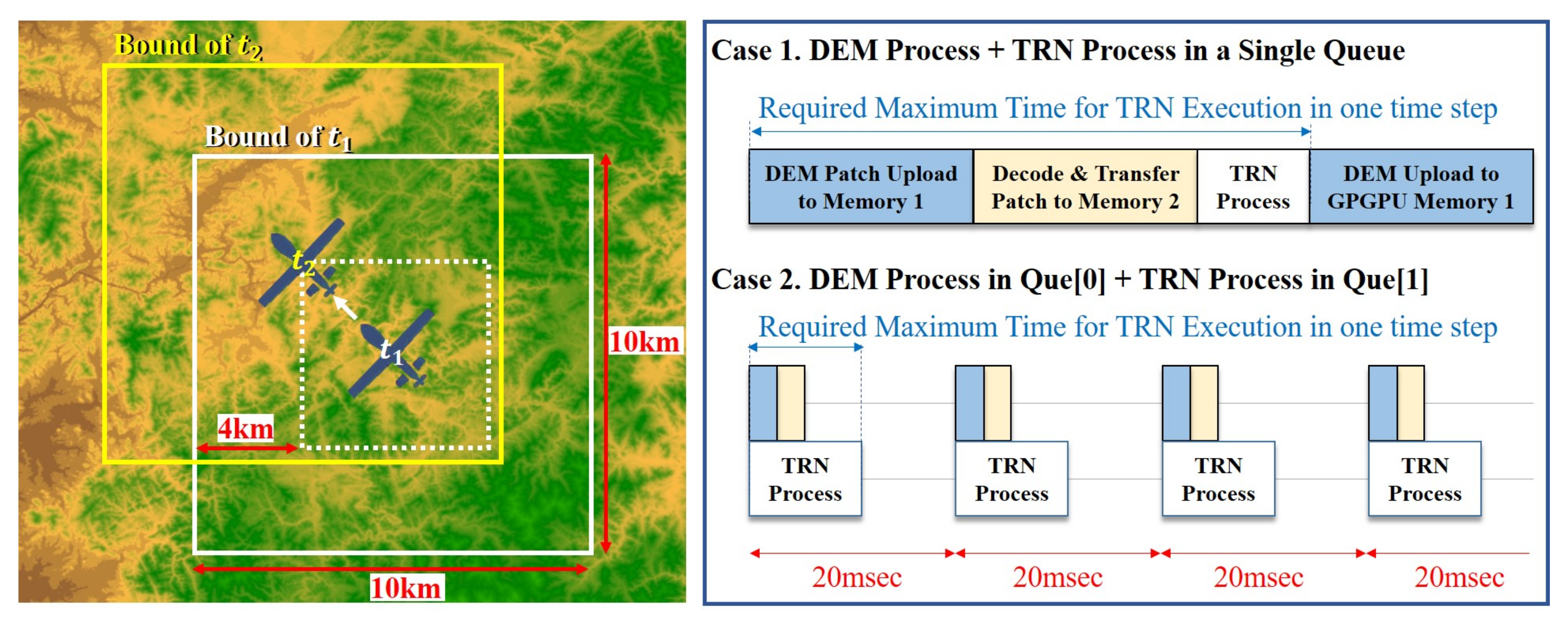
A high-resolution DEM is an essential element for improving the performance of TRN. However, large amounts of memory space are needed to store a high-resolution DEM and additional time is needed to load the DEM in a separate storage space [34]. In the past, the memory capacity of the navigation computer was insufficient, so only part of the DEM around the pre-planned route was loaded into the memory [35]. In this study, we applied a 64 GB solid-state drive (SSD) to store 3 m resolution digital terrain elevation data (DTED) level 4 in the mission area and 10 m resolution DTED level 3 in the rest of the flight area. At the Korean peninsula area, DTED level 4 requires about 15 GB of memory space and DTED level 3 requires about 3.7 GB of memory space. As these high-resolution terrain DBs are large files, they are difficult to process in real-time. Typically, as the AMD E8860 GPGPU, where the TRN algorithm performs, has a 2 GB synchronous dynamic random access memory (SDRAM), it is impossible to load the entire DEM.

Therefore, in this study, as shown in Figure 5, the DEM patch corresponding to a 10 km × 10 km area is generated based on the current estimated position of the aircraft in the CPU, and then transferred to the SDRAM of the GPGPU. For the aircraft flight from $t_1$ to $t_2$ in Figure 5, there is a 4 km difference from the boundary of the DEM patch generated at the point $t_1$. At this time, another DEM patch with a 10 km × 10 km area is generated at point $t_2$. When a DEM patch is generated, the highest resolution DEM among the available DEMs present in the region is selected, and one patch may be made of a combination of several DEMs. When combining DEMs with more than two resolutions, the boundary processing uses the linear interpolation method. Two buffers are created in the GPGPU’s memory for the purpose of storing DEM patches. One (Memory 2 in Figure 5) stores the DEM patch used in the TRN algorithm, and the other (Memory 1 in Figure 5) loads the newly generated DEM patch. When loading of the new DEM patch in Memory 1 is completed, the DEM patch is decoded. This is because the high-resolution DEM is encoded so that the terrain DB can be completely preserved from enemies even when the aircraft crashes. After the decoding step, the new DEM patch must be moved to Memory 2 for the TRN algorithm. If the DEM and TRN processes sequentially, as in Case 1 of Figure 5, and the maximum time of one TRN loop execution exceeds 20 msec, then real-time computation is not guaranteed. Therefore, in this study, two queues (Que[0] and Que[1]) were created in GPGPU as in Case 2 of Figure 5, and the DEM and TRN are processed using a task parallel computing method. The DEM processing itself was also divided in order to prevent the moment of accessing Memory 2 at the same time as the TRN processing.

4. Verification of a Three-Dimensional Terrain Based System

4.1. Experiment Results in a SIL Environment

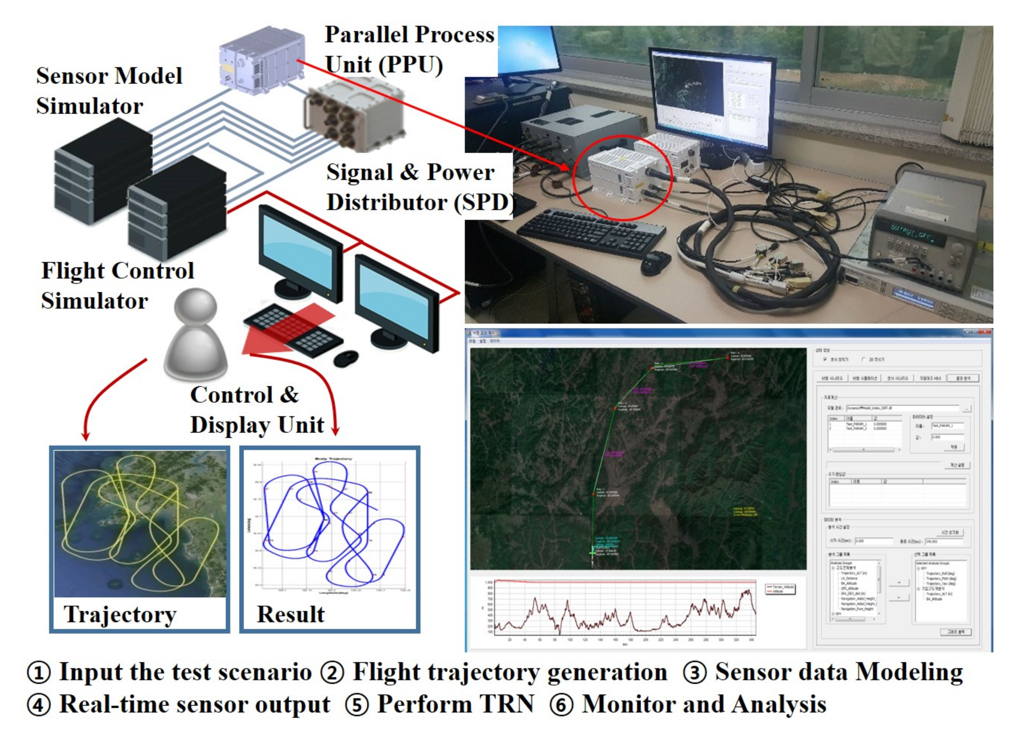
Before the proposed AP-TAN is applied to UAVs, we investigated the feasibility of the navigation performance on a real aircraft platform. As the verification on the aircraft platform through captive flight tests is expensive, the pre-verification through Monte Carlo offline simulation or SIL tests is necessary. In particular, this section deals with SIL test results for real-time verification of the proposed navigation software on the PPU prior to flight tests. Among the navigation algorithms, inertial navigation and INS/GNSS-aided navigation can generally be verified by vehicle testing. However, because the IRA is inoperable on the ground, we developed the SIL test equipment, shown in Figure 6, to verify the TRN and INS/TRN aided navigation.

The main functions of the equipment are the creation of flight scenarios (Flight Control Simulator in Figure 6), the generation of simulated sensor data along the scenarios (Sensor Model Simulator in Figure 6), the real-time outputs of the generated signals, and the analysis of navigation results carried out on a PPU (Control and Display Unit in Figure 6). The SPD in Figure 6 delivers the commands from the control and display unit and the sensor data from the sensor model simulator to the PPU, and delivers the navigation results from the PPU to the control and display unit. In addition, real-time simulations using sensor data and flight trajectory data acquired through captive flight tests can be performed, so the proposed system has been continuously validated and modified through the SIL tests. As the modeling of the IRA is the most important sensor in the proposed system, we developed a sensor model simulator including the IRA signal processing method and verified the simulator through captive flight tests.

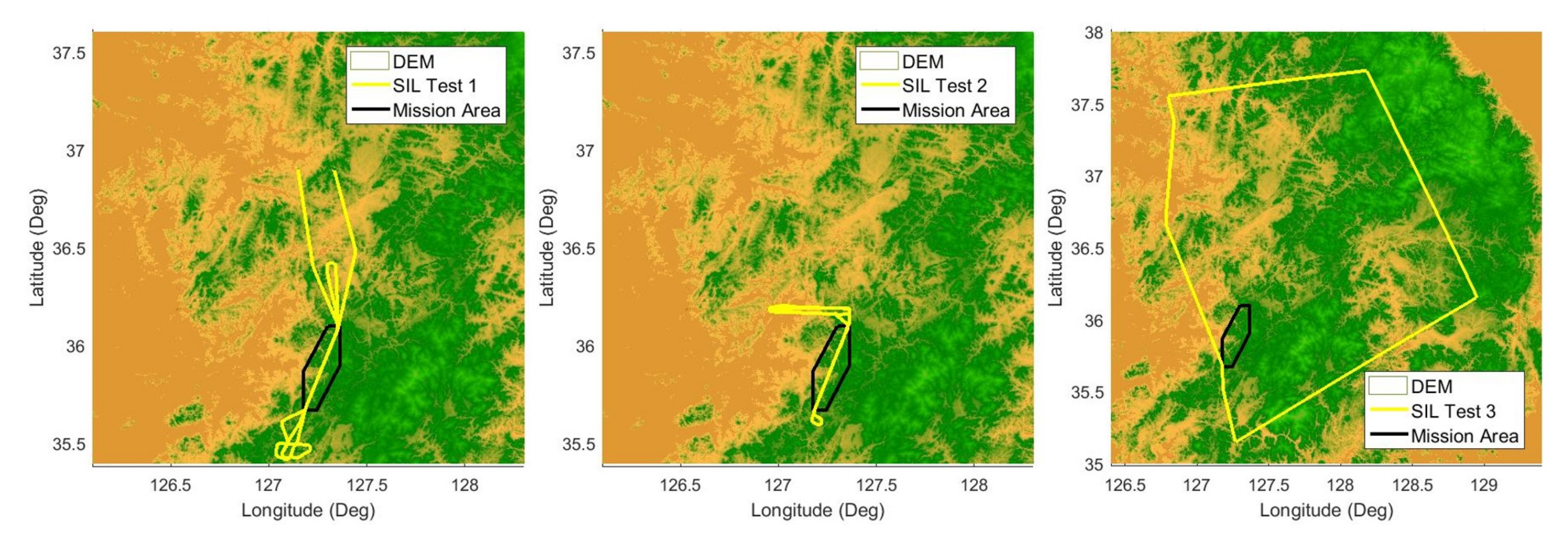
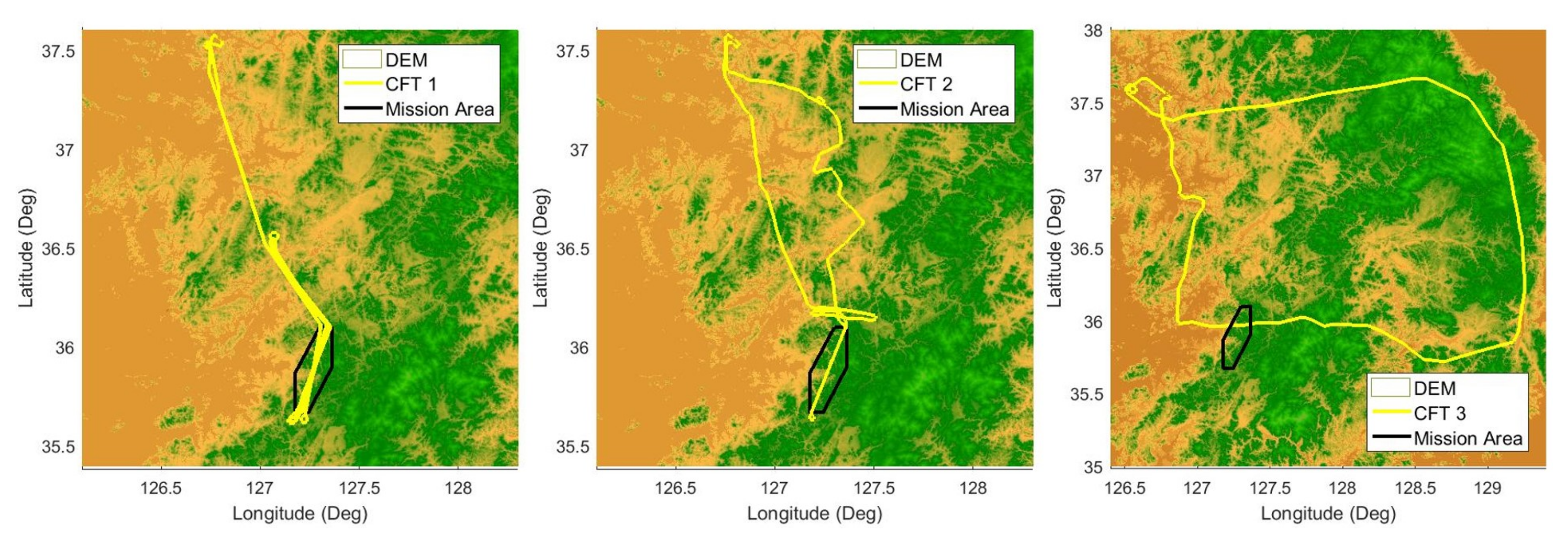
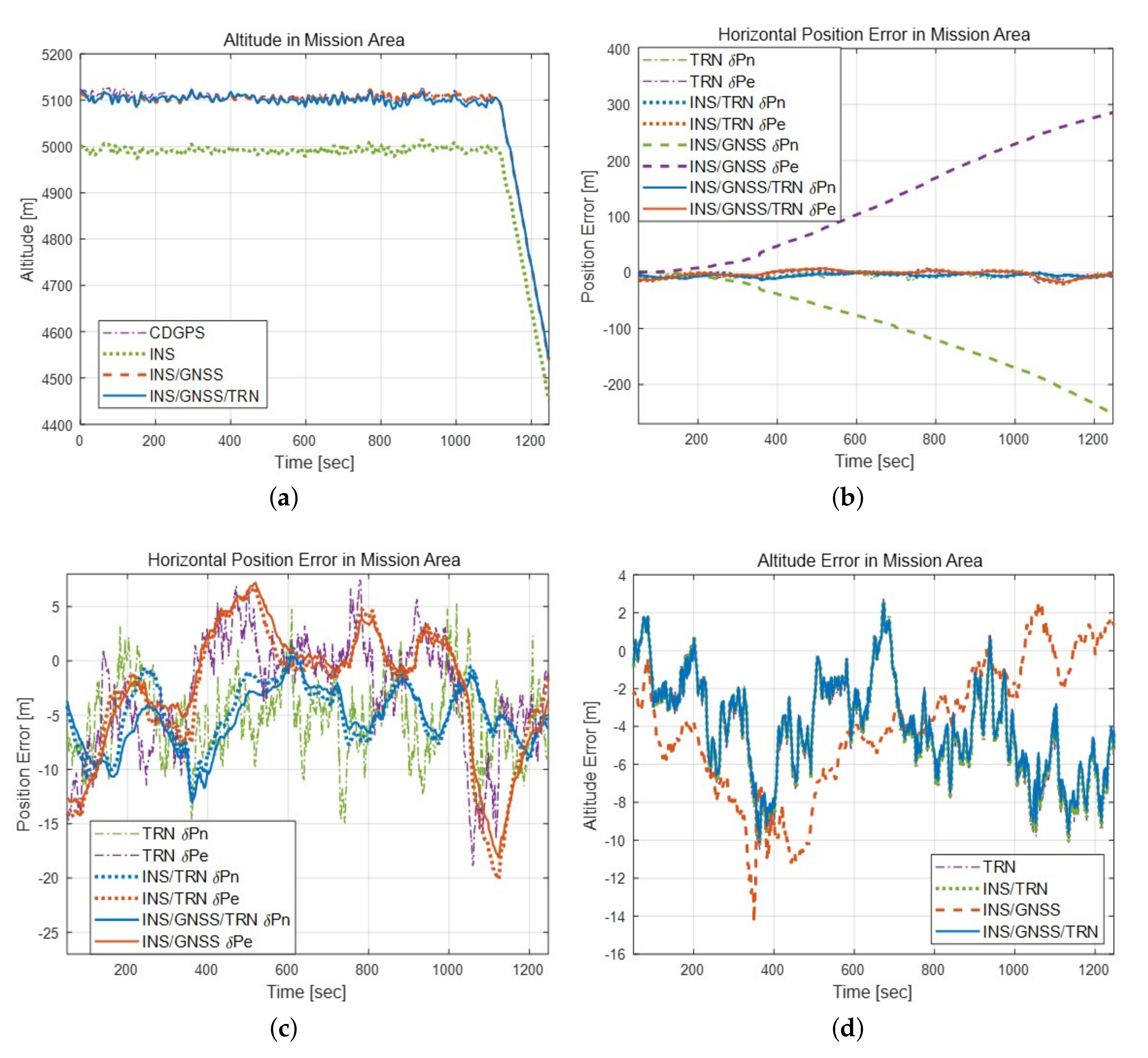
Figure 7 and

Table 1. Simulation conditions of the SIL tests.

No. of Test	Total Flight Time	Mission Time	Flight Altitude	GNSS Unavailable Area
SIL Test 1	1 h.  20 min.	13 min.	1.3 km	Mission Area
SIL Test 2	42 min.	23 min.	5.3 km	Mission Area
SIL Test 3	1 h.  50 min.	1 hr.  40 min.	2.3 km	Whole Area

show flight trajectories and simulation conditions for three SIL tests. The area enclosed by black lines in Figure 7 is the mission area, and the 3m resolution DTED level 4 was constructed using light detection and ranging (LiDAR) equipment. The 10 m resolution DTED Level 3 was used for the remaining. The mission area was chosen close to the runway after excluding urban areas, flat areas such as seas and rivers, and military training areas. In SIL Tests 1 and 2, the GNSS was set to be not available within the mission area, and the GNSS was set to be available again after leaving the mission area. On the other hand, in Test 3, GNSS was set to be unavailable after the aircraft had risen above 1km. As shown in Table 1, the average flight altitudes of SIL Tests 1, 2, and 3 were set to 1.3 km, 5.3 km, and 2.3 km, respectively. When GNSS is not available, the INS/GNSS-aided navigation only performs a propagation.

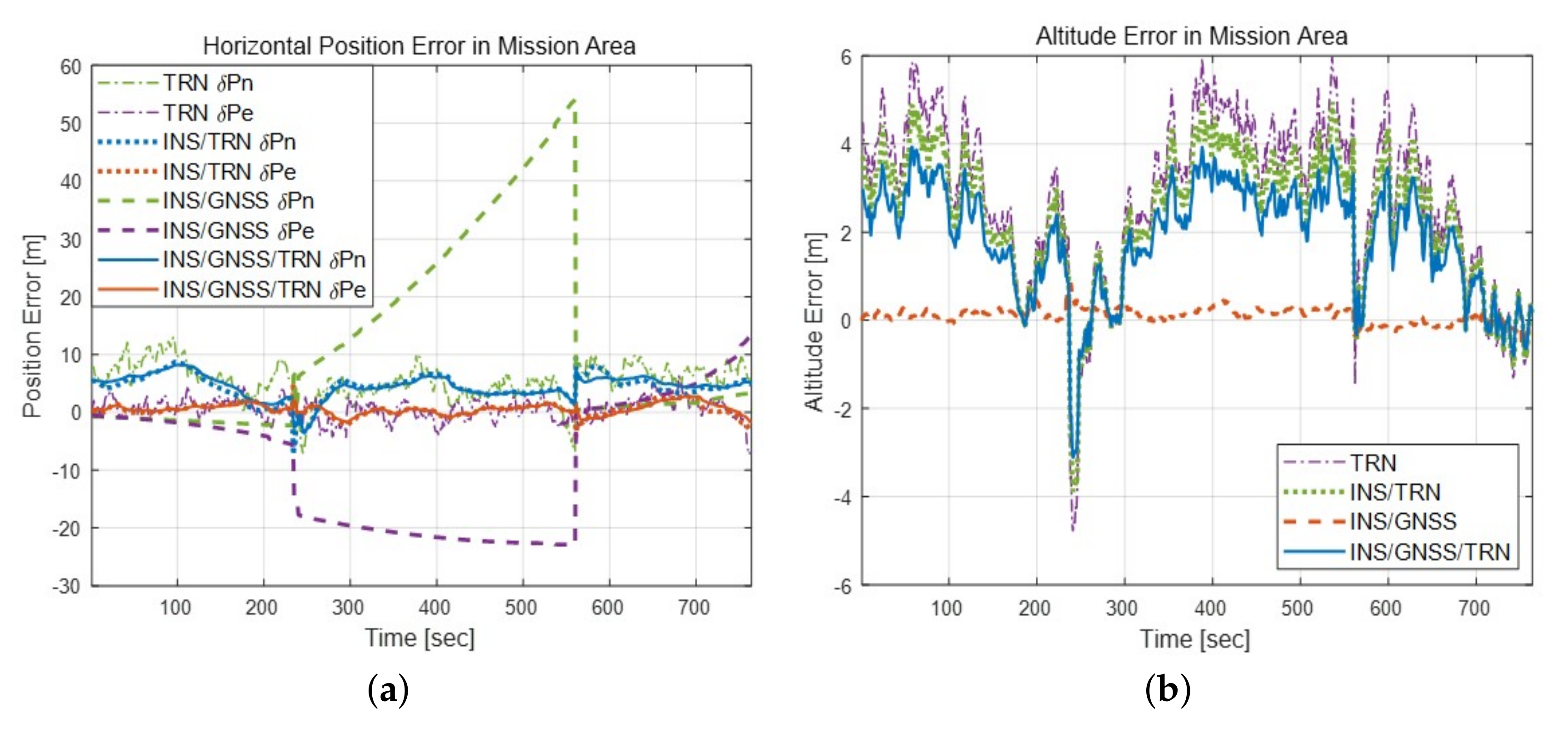
As INS/GNSS-aided navigation has been validated in many previous studies, we dealt with the results of the performance analysis on a mission area on which TRN was performed and GNSS was unavailable. For SIL Test 3, we performed TRN simulation without GNSS for all flight times except for take-off time. The simulation results are shown in Figure 8, Figure 9 and Figure 10 and

Table 2. Simulation results of the SIL tests in a GNSS-denied environment.

Hor. Pos. Error [m CEP]	SIL Test 1	SIL Test 2	SIL Test 3
TRN	4.89 m	6.74 m	9.13 m
INS/TRN	3.54 m	5.62 m	7.23 m
INS/GNSS	20.06 m	39.52 m	2242.68 m
INS/GNSS/TRN	3.50 m	5.43 m	6.73 m
Altitude Error [m PE]	SIL Test 1	SIL Test 2	SIL Test 3
TRN	2.29 m	1.35 m	1.49 m
INS/TRN	1.91 m	1.13 m	1.35 m
INS/GNSS	0.14 m	1.86 m	0.26 m
INS/GNSS/TRN	1.53 m	0.90 m	1.18 m

. For SIL Test 1, three tests were conducted in the mission area, and the test resumed after a long flight without GNSS before entering the second mission area. This was done to analyze the effect of the absence of GNSS for a long time on TRN. For this reason, the slope of the INS/GNSS-aided navigation error increased rapidly in the second test section of Figure 8a, but this did not affect the TRN. Because GNSS was temporarily available before flying into the mission area, there was a moment when the INS/GNSS-aided navigation error decreased between the three missions, as shown in Figure 8a. In SIL Test 1, the inertial navigation altitude through the 3rd damping loop was stable because no error is applied to the barometer model, and the altitude performance of the INS/GNSS-aided navigation is stable as shown in Figure 8b. On the other hand, the altitude error of TRN was relatively large, but it was due to the discrepancy between the altitude bias model predicted by the APF and the ideal barometer model without error.

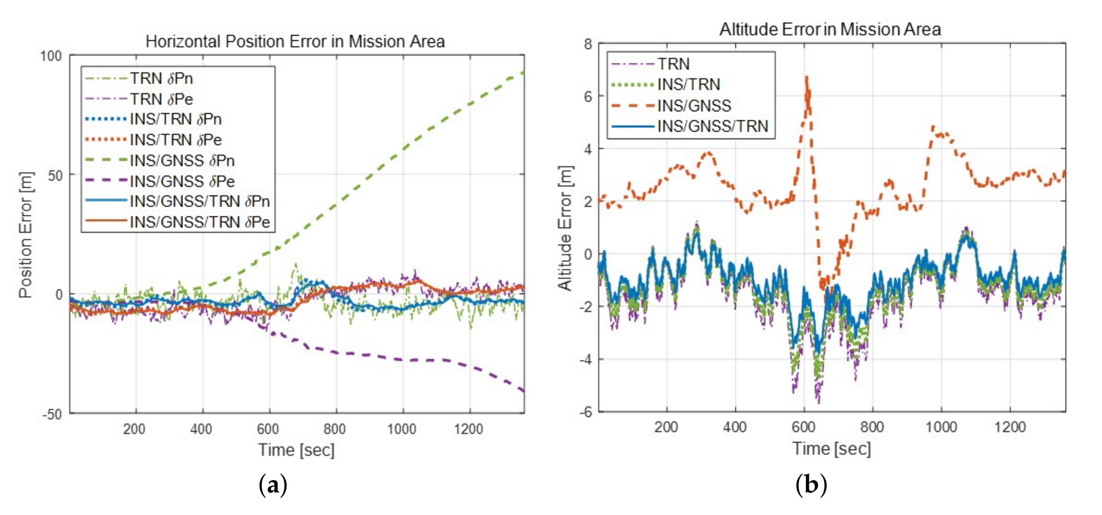
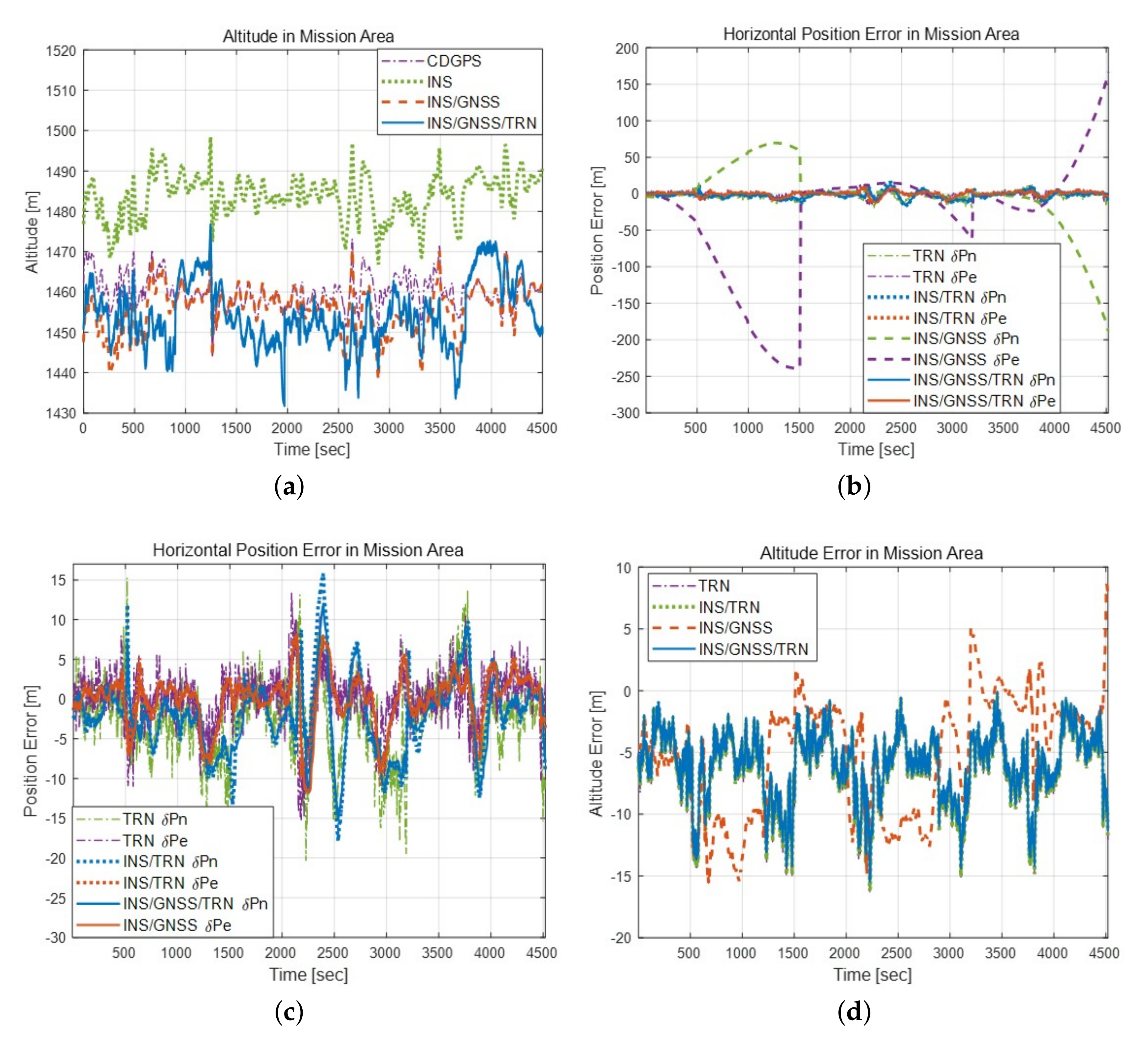
As shown in Figure 9, SIL Test 2 was the simulation result using real flight test data with an average flight altitude of 5.3 km. As the trajectory data used in the simulation, the carrier differential global positioning system (CDGPS) data obtained from the real flight test was used. For SIL Test 2, one test was conducted in the mission area. Comparing Figure 8a and Figure 9a shows that the TRN performance was somewhat degraded as the altitude increased, but the navigation results were stable even in the GNSS unavailable environment. In addition, unlike in Figure 8b, Figure 9b shows that when we used real flight data with a barometer error, the altitude error of TRN was properly estimated. As shown in Figure 8a and Figure 9a, the INS/GNSS/TRN integrated navigation performed slightly better than the INS/TRN aided navigation when the GNSS error was small, even in the GNSS available environment. However, as the GNSS error increased the performance was almost equivalent to that of the INS/TRN-aided navigation. In SIL Test 3, a TRN simulation was performed in over the entire Korean peninsula using 10 m resolution DTED Level 3.

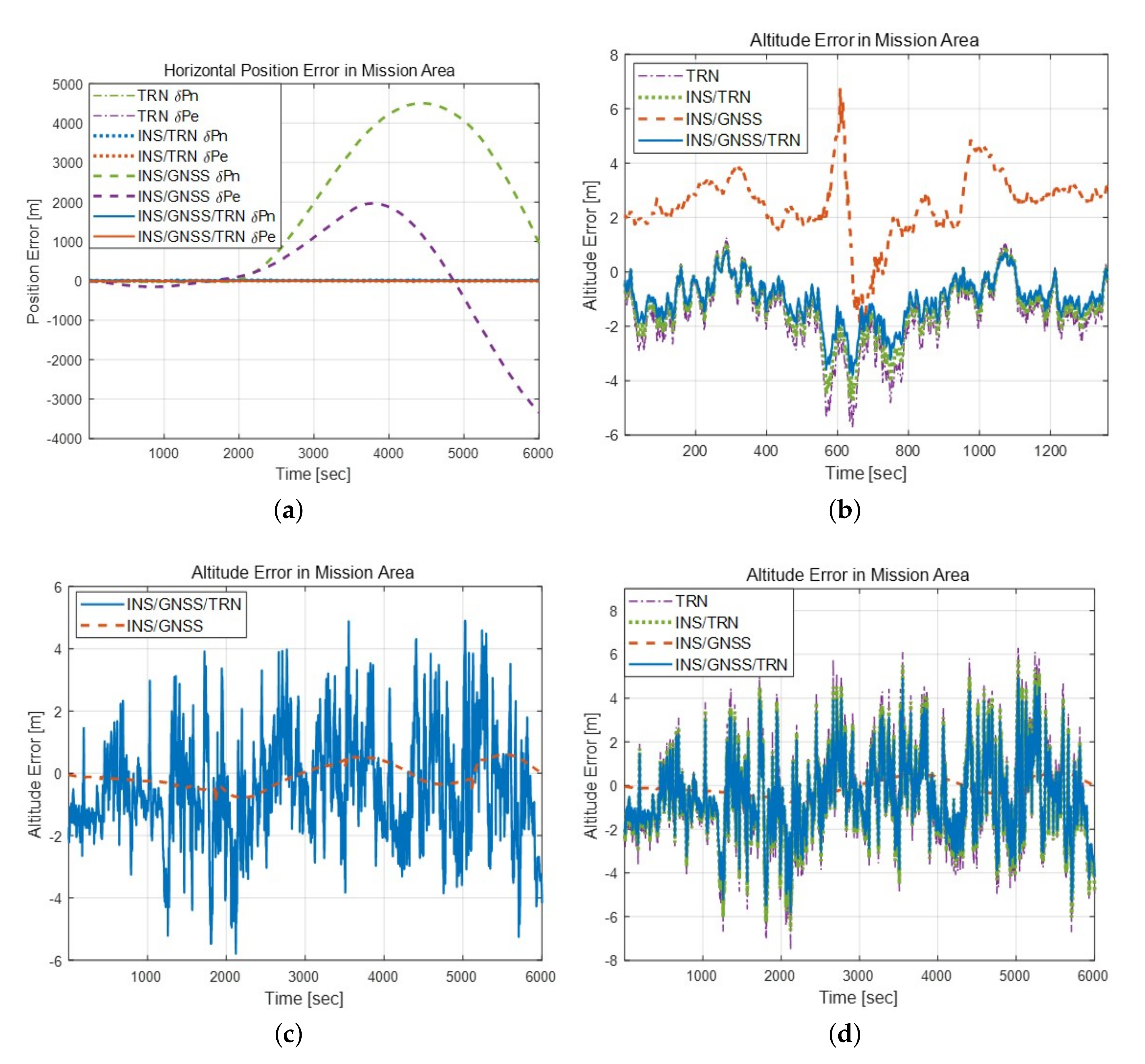
As shown in Figure 10a, because GNSS was unavailable during one hour and 40 min of flight time, the INS/GNSS-aided navigation error increased significantly to the inertial navigation level. In contrast, both the INS/TRN-aided navigation and INS/GNSS/TRN integrated navigation maintained stable performance. As shown in Figure 10b, the INS/TRN performance was degraded because the enough terrain roughness for the reliable TRN performance was not guaranteed between 100 and 1400 s through urban areas. However, it can be seen that the performance of the INS/TRN-aided navigation was restored soon after the roughness was secured. As shown in Figure 10c,d, the INS/TRN-aided navigation and INS/GNSS/TRN integrated navigation altitude errors were generally stable, although they were somewhat larger than the INS/GNSS-aided navigation altitude error, which was almost the same as the barometer’s third damping loop output.

Table 2 reveals that the SIL Test 1 with 3 m resolution DTED Level 4 had a 3.54 m circular error probability (CEP) for the INS/TRN-aided navigation and a 3.50 m CEP for the INS/GNSS/TRN integrated navigation at a 1.3 km flight altitude. Moreover, the SIL Test 2 with 3 m resolution DTED Level 4 had a 5.62 m CEP for the INS/TRN-aided navigation and a 5.43 m CEP for the INS/GNSS/TRN integrated navigation at a 5.3 km flight altitude. Even under conditions where the GNSS was unavailable for one hour and 40 min, the SIL Test 3 with 10 m resolution DTED Level 3 had a 7.23 m CEP for the INS/TRN-aided navigation and a 6.73 m CEP for the INS/GNSS/TRN integrated navigation at a 2.3 km flight altitude. In addition, in all SIL tests, the TRN acquisition mode by batch processing delivered a coarse position with errors less than a 30 m CEP within 40 s in the APF-based TRN tracking mode.

4.2. Verification Using Captive Flight Tests

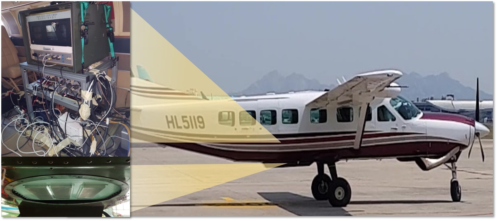
Captive flight test techniques include a full range of techniques for verifying real-time inertial navigation, integrated navigation and TRN performance by equipping a real aircraft with the proposed AP-TAN. In this study, we designed and manufactured a testbed including an IRA, an INS, a GNSS receiver, a barometer, a PPU, and a SPD, as shown in Figure 11. Prior to the test evaluation, digital surface model (DSM) and DEM with a 3m resolution were constructed using LiDAR. The captive flight tests used a CESSNA 172 Skyhawk with a hole to mount the IRA antenna on the bottom of the fuselage as shown in Figure 11. To minimize the mounting errors between the IRA antenna assembly and the INS, the testbed was manufactured to be mounted on the same mounting plate. The IRA antenna assembly was installed at the bottom of the mounting plate towards the ground. The INS was installed on the opposite side of the plate where the IRA antenna assembly was installed. All other equipments were mounted inside the aircraft using a separate rack. The PPU developed in this study was equipped with an $\times 86$ series i7-4799EQ SBC with a 8 GB DDR3 memory, AMD E8860 embedded GPGPU, and 64 GB SSD for high-resolution DEMs. In the SBC, inertial navigation and integrated navigation were performed, whereas TRN and DEM real-time processing were performed in the GPGPU board. The GNSS measurements obtained by compensating the lever arm between the GNSS antenna and the INS were used. In addition, the mounting misalignment angle between the INS and the IRA antenna was measured and this misalignment angle was compensated when converting the IRA measurement into the three-dimensional relative distance on the ENU coordinate. The threshold of the misalignment angle error was set to ~${0.1}^{\circ }$ through simulations and the measured error was ~${0.032}^{\circ }$.

In this section, we analyze the results of three system performance evaluation tests when a GNSS was not available, as shown in

Table 3. Conditions of captive flight tests.

No. of Test	Total Flight Time	Mission Time	Flight Altitude	GNSS Unavailable Area
CFT 1	3 hr. 33 min.	1 hr. 58 min.	1.5 km	Mission Area
CFT 2	2 hr. 33 min.	23 min.	5.1 km	Mission Area
CFT 3	3 hr. 40 min.	1 hr. 42 min.	1.3 km∼3.3 km	Whole Area

and Figure 12. The three flight tests had the same purpose as the SIL tests mentioned in Section 4.1 above. However, in the case of CFT 3, unlike in the SIL Test 3, the flight altitude was freely determined by the operator within a range of 1.3 km to 3.3 km. The shorter mission time than flight time in CFT 2 was due to the long waiting time for entry permission into the mission area. On the other hand, in the case of CFT 3, the waiting time was necessary to confirm whether the proposed system operates normally even when the GNSS is unavailable for a long time.

Figure 13, Figure 14 and Figure 15 below show the results of the three CFTs. For the objectivity of test evaluation, the CDGPS data was logged during captive flight test, postprocessed, and used as reference data. In Figure 13a, Figure 14a and Figure 15a, the INS altitude represents the barometer’s third damping loop output. As shown in Figure 13a, the INS altitude error was about 15.99 m probable error (PE) compared to CDGPS data at a 1.4 km flight altitude. On the other hand, the remaining TRN and integrated navigation show similar performance within 5 m PE. Based on these results, we can confirm that the proposed barometer error compensation scheme works in a real environment. As shown in Figure 13b, the CFT 1 performed three tests in the mission area. Before each test set, the GNSS was made available temporarily and then re-entered into the mission area and was again unavailable. Accordingly, the INS/GNSS integrated navigation error decreased momentarily at 1500 s and 3250 s and then increased continuously after entering the mission area as shown in Figure 13b. On the other hand, as shown in Figure 13c,d, the TRN, INS/TRN-aided navigation and INS/GNSS/TRN integrated navigation provided stable performances at a flight altitude of 1.5 km when GNSS was unavailable. However, even if the terrain was rough enough, the IRA availability decreased at 1500 s and 3250 s when the aircraft was turning, leading to poor performance of the TRN, as shown in Figure 13a.

Figure 14a shows that the INS altitude error was about 92.74 m PE compared to the CDGPS data at a 5.1 km flight altitude. Comparing Figure 13a and Figure 14a reveals that the INS altitude error of CFT 2 was larger than that of CFT 1. This was because there was a barometer scale factor error, so the altitude error for flying at 5.1 km was larger than for flying at 1.5 km. In addition, the scale factor error of the barometer was affected not only by altitude, but also by temperature. In the case of CFT 2, as the waiting time increased before the mission was performed, the temperature deviation between the takeoff and the mission was large, which resulted in a larger INS altitude error. On the other hand, the remaining TRN and integrated navigation had similar performances within 4 m PE. Based on these results, we can confirm that the proposed barometer error compensation scheme works in a real environment. As shown in Figure 14b, the CFT 2 performed one test in the mission area in consideration of flight safety under the restrictions of operating with an oxygen mask at altitudes above 5 km. The INS/GNSS integrated navigation error increased continuously after entering the mission area. On the other hand, as shown in Figure 14c,d, the TRN, INS/TRN-aided navigation and INS/GNSS/TRN integrated navigation provided stable performances at a flight altitude of 5.1 km when GNSS was unavailable.

As shown in Figure 15a, the INS altitude error was ~12.47 m PE compared to CDGPS data. On the other hand, the remaining TRN and integrated navigation had similar performances within 7 m PE. The CFT 1 and 2 were performed during a level flight, but in the case of the CFT 3, the altitude error was slightly increased because it was freely flown between 1.3 km and 3.3 km altitudes as shown in Figure 15d, but the results were improved compared to the third damping loop output. In Figure 15b, the INS/GNSS integrated navigation error increases continuously after entering the mission area. On the other hand, as shown in Figure 15c,d, the TRN, INS/TRN-aided navigation and INS/GNSS/TRN integrated navigation provide stable performances at any flight altitude when GNSS is unavailable. As shown in Figure 15d, when the altitude changes, the longer the GNSS is unavailable, the larger the altitude error of INS/GNSS-aided navigation. On the other hand, the altitude of INS/TRN-aided navigation showed stable performance even with altitude change.

Table 4. Batch processing-based TRN acquisition position error of the captive flight tests.

No. of Test	Acquisition Time	Latitude Error	Longitude Error
CFT 1	47 sec	5 m	3.5 m
CFT 2	30 sec	−10 m	−10 m
CFT 3	24 sec	−16 m	−1 m

below summarizes the TRN acquisition results based on batch processing. In CFT 1, the conditions for converting from acquisition mode to tracking mode were so severe that the coarse position error was small but the acquisition time was slightly longer. Therefore, the conversion conditions were designed to be alleviated as shown in Equations (21) and (22) of Section 3.2 so that the acquisition time would be within 30 s. The position root mean square (RMS) errors of acquisition mode were within 20 m.

Table 5. Experiment results of the captive flight tests in a GNSS-denied environment.

Hor. Pos. Error [m CEP]	CFT 1	CFT 2	CFT 3
TRN	3.97 m	6.45 m	9.85 m
INS/TRN	3.07 m	5.90 m	8.87 m
INS/GNSS	78.92 m	164.85 m	1212.85 m
INS/GNSS/TRN	3.75 m	6.28 m	8.39 m
Altitude Error [m PE]	CFT 1	CFT 2	CFT 3
TRN	4.62 m	3.33 m	6.79 m
INS/TRN	4.60 m	3.29 m	6.74 m
INS/GNSS	4.76 m	3.62 m	6.47 m
INS/GNSS/TRN	4.46 m	3.16 m	6.48 m

summarizes the navigation results of CFTs in a GNSS unavailable environment. Applying DTED Level 4 in a GNSS unavailable environment, Table 5 shows a 3.07 m CEP and a 5.90 m CEP for INS/TRN-aided navigation errors at 1.4 km and 5.1 km, respectively. On the other hand, when DTED Level 3 was applied, the error of the INS/TRN-aided navigation was 8.87 m CEP. In addition, even if there were many barometer errors, the altitude of the proposed system had a stable performance.

5. Conclusions

In this study, we introduced the AP-TAN, which can be used even in environments where a GNSS is unavailable or terrain roughness cannot be determined. First, an IRA was used as the altimeter of the proposed system, and a suitable error compensation method was introduced. Next, to secure UAV survivability and reliability in an environment where a GNSS is unavailable for a long time, we developed an optimal combination TRN algorithm consisting of an acquisition mode based on batch processing and a tracking mode based on an APF. In order to improve the performance of TRN, a high-resolution DEM was constructed. A GPGPU-based parallel computing technology was applied to deal with a large amount of computational APF-based TRN and high-resolution DEM real-time processing. We also developed the INS/GNSS/TRN integrated navigation based on the federated filter to guarantee the navigation performance even in environments where either GNSS or TRN is unavailable. Finally, SIL tests and CFTs were performed to verify the performance of the proposed system when GNSS was denied. As a result, an INS/TRN-aided navigation performance of about a 3.1 m CEP at 1.5 km flight altitude and about a 5.9 m CEP at 5.1 km altitude was obtained using 3 m resolution DTED. Moreover, the INS/TRN/GNSS integrated navigation performance of about 8.4 m CEP was obtained using 10 m resolution DTED between 1.3 km to 3.3 km altitude when there is no GNSS for about two hours. Based on the test results of the proposed system, it was confirmed that reliable navigation performance can be obtained through the TRN even in environments where the GNSS is not available. Moreover, it has been shown that the AP-TAN can be applied to UAV for surveillance and reconnaissance purposes by verifying the performance of an IRA-based TRN at various altitudes ranging from 1 km to 5 km. Of course, in situations where the GNSS and TRN are not available at the same time, as only pure navigation is performed, the error increased over time. However, the proposed federated filter-based integrated navigation system has the advantages that it is easy to add the various aiding sensors to solve the problem and to detect and separate the faulty sensors. Further, the proposed hybrid TRN algorithm can also be applied to autonomous underwater vehicles (AUVs).

References

- Grewal, M.S.; Weill, L.R.; Andrews, A.P. Global Positioning Systems, Inertial Navigation, and Integration; John Wiley & Sons: Hoboken, NJ, USA, 2007. [Google Scholar]
- Zhang, G.; Hsu, L.T. Intelligent GNSS/INS integrated navigation system for a commercial UAV flight control system. Aerosp. Sci. Technol. 2018, 80, 368–380. [Google Scholar] [CrossRef]
- Courbon, J.; Mezouar, Y.; Guénard, N.; Martinet, P. Vision-based navigation of unmanned aerial vehicles. Control Eng. Pract. 2010, 18, 789–799. [Google Scholar] [CrossRef]
- Belmonte, L.M.; Morales, R.; Fernández-Caballero, A. Computer Vision in Autonomous Unmanned Aerial Vehicles—A Systematic Mapping Study. Appl. Sci. 2019, 9, 3196. [Google Scholar] [CrossRef] [Green Version]
- Konovalenko, I.; Kuznetsova, E.; Miller, A.; Miller, B.; Popov, A.; Shepelev, D.; Stepanyan, K. New approaches to the integration of navigation systems for autonomous unmanned vehicles (UAV). Sensors 2018, 18, 3010. [Google Scholar] [CrossRef] [Green Version]
- Popp, M.; Scholz, G.; Prophet, S.; Trommer, G. A laser and image based navigation and guidance system for autonomous outdoor-indoor transition flights of MAVs. In Proceedings of the 2015 DGON Inertial Sensors and Systems Symposium (ISS), Karlsruhe, Germany, 22–23 September 2015; IEEE: Hoboken, NJ, USA, 2015; pp. 1–18. [Google Scholar]
- Thoma, J.; Paudel, D.P.; Chhatkuli, A.; Probst, T.; Gool, L.V. Mapping, localization and path planning for image-based navigation using visual features and map. In Proceedings of the IEEE Conference on Computer Vision and Pattern Recognition, Long Beach, CA, USA, 15–20 June 2019; pp. 7383–7391. [Google Scholar]
- Melo, J.; Matos, A. Survey on advances on terrain based navigation for autonomous underwater vehicles. Ocean Eng. 2017, 139, 250–264. [Google Scholar] [CrossRef] [Green Version]
- Jeon, H.C.; Park, W.J.; Park, C.G. Grid design for efficient and accurate point mass filter-based terrain referenced navigation. IEEE Sensors J. 2017, 18, 1731–1738. [Google Scholar] [CrossRef]
- ZELENKA, R. Integration of radar altimeter, precision navigation, and digital terrain data for low-altitude flight. In Proceedings of the Guidance, Navigation and Control Conference, Hilton Head Island, SC, USA, 10–12 August 1992; p. 4420. [Google Scholar]
- Oh, J.; Sung, C.K.; Lee, J.; Lee, S.W.; Lee, S.J.; Yu, M.J. Accurate Measurement Calculation Method for Interferometric Radar Altimeter-Based Terrain Referenced Navigation. Sensors 2019, 19, 1688. [Google Scholar] [CrossRef] [Green Version]
- Hager, J.R.; Almsted, L.D. Methods and Systems for Enhancing Accuracy of Terrain Aided Navigation Systems. U.S. Patent 7,409,293, 5 August 2008. [Google Scholar]
- Turan, B.; Kutay, A.T. Particle filter studies on terrain referenced navigation. In Proceedings of the 2016 IEEE/ION Position, Location and Navigation Symposium (PLANS), Savannah, GA, USA, 11–14 April 2016; IEEE: Hoboken, NJ, USA, 2016; pp. 949–954. [Google Scholar]
- Lee, J.; Bang, H. A robust terrain aided navigation using the Rao-Blackwellized particle filter trained by long short-term memory networks. Sensors 2018, 18, 2886. [Google Scholar] [CrossRef] [Green Version]
- Groves, P.D.; Handley, R.J.; Runnalls, A.R. Optimising the integration of terrain referenced navigation with INS and GPS. J. Navig. 2006, 59, 71–89. [Google Scholar] [CrossRef]
- Peters, M.A. Development of a TRN/INS/GPS integrated navigation system. In Proceedings of the IEEE/AIAA 10th Digital Avionics Systems Conference, Los Angeles, CA, USA, 14–17 October 1991; IEEE: Hoboken, NJ, USA, 1991; pp. 6–11. [Google Scholar]
- Salavasidis, G.; Munafò, A.; Harris, C.A.; Prampart, T.; Templeton, R.; Smart, M.; Roper, D.T.; Pebody, M.; McPhail, S.D.; Rogers, E.; et al. Terrain-aided navigation for long-endurance and deep-rated autonomous underwater vehicles. J. Field Robot. 2019, 36, 447–474. [Google Scholar] [CrossRef] [Green Version]
- Yang, L. Reliability Analysis of Multi-Sensors Integrated Navigation Systems. Ph.D. Thesis, University of New South Wales, Sydney, Australia, August 2014. [Google Scholar]
- Luyang, T.; Xiaomei, T.; Huaming, C.; Xiaohui, L. An Adaptive Federated Filter in Multi-source Fusion Information Navigation System. IOP Conf. Ser. Mater. Sci. Eng. 2018, 392, 062195. [Google Scholar] [CrossRef]
- Carlson, N.A. Federated square root filter for decentralized parallel processors. IEEE Trans. Aerosp. Electron. Syst. 1990, 26, 517–525. [Google Scholar] [CrossRef]
- Carlson, N.A.; Berarducci, M.P. Federated Kalman filter simulation results. Navigation 1994, 41, 297–322. [Google Scholar] [CrossRef]
- Seo, J.; Lee, J.G.; Park, C.G. A New error compensation scheme for INS vertical channel. IFAC Proc. Vol. 2004, 37, 1119–1124. [Google Scholar] [CrossRef]
- Lee, J.; Sung, C.; Park, B.; Lee, H. Design of INS/GNSS/TRN Integrated Navigation Considering Compensation of Barometer Error. J. Korea Inst. Mil. Sci. Technol. 2019, 22, 197–206. [Google Scholar]
- Jeong, S.H.; Yoon, J.H.; Park, M.G.; Kim, D.Y.; Sung, C.K.; Kim, H.S.; Kim, Y.H.; Kwak, H.J.; Sun, W.; Yoon, K.J. A performance analysis of terrain-aided navigation (TAN) algorithms using interferometric radar altimeter. J. Korean Soc. Aeronaut. Space Sci. 2012, 40, 285–291. [Google Scholar]
- Lee, J.; Bang, H. Radial basis function network-based available measurement classification of interferometric radar altimeter for terrain-aided navigation. IET Radar Sonar Navig. 2018, 12, 920–930. [Google Scholar] [CrossRef]
- Yoo, Y.M.; Lee, S.M.; Kwon, J.H.; Yu, M.J.; Park, C.G. Profile-based TRN/INS integration algorithm considering terrain roughness. J. Inst. Control. Robot. Syst. 2013, 19, 131–139. [Google Scholar] [CrossRef] [Green Version]
- Candy, J.V. Bayesian Signal Processing: Classical, Modern, and Particle Filtering Methods; John Wiley & Sons: Hoboken, NJ, USA, 2016; Volume 54. [Google Scholar]
- Pitt, M.K.; Shephard, N. Filtering via simulation: Auxiliary particle filters. J. Am. Stat. Assoc. 1999, 94, 590–599. [Google Scholar] [CrossRef]
- Teixeira, F.C.; Quintas, J.; Pascoal, A. AUV terrain-aided navigation using a Doppler velocity logger. Annu. Rev. Control 2016, 42, 166–176. [Google Scholar] [CrossRef]
- Teixeira, F.C.; Quintas, J.; Maurya, P.; Pascoal, A. Robust particle filter formulations with application to terrain-aided navigation. Int. J. Adapt. Control Signal Process. 2017, 31, 608–651. [Google Scholar] [CrossRef]
- Han, K.J.; Sung, C.K.; Yu, M.J.; Park, C.G. Performance improvement of laser TRN using particle filter incorporating gaussian mixture noise model and novel fault detection algorithm. In Proceedings of the ION/GNSS+ 2018 the 31st International Technical Meeting of the Satellite Division of the Institute of Navigation, Miami, FL, USA, 24–28 September 2018; ION: Washington, DC, USA, 2018; pp. 3317–3326. [Google Scholar]
- Munshi, A.; Gaster, B.; Mattson, T.G.; Ginsburg, D. OpenCL Programming Guide; Pearson Education: London, UK, 2011. [Google Scholar]
- Yigit, H.; Yilmaz, G. Development of a GPU accelerated terrain referenced UAV localization and navigation algorithm. J. Intell. Robot. Syst. 2013, 70, 477–489. [Google Scholar] [CrossRef]
- Lee, J.; Sung, C.; Oh, J. Terrain Referenced Navigation Using a Multilayer Radial Basis Function-Based Extreme Learning Machine. Int. J. Aerosp. Eng. 2019, 2019. [Google Scholar] [CrossRef] [Green Version]
- Chen, X.; Wang, C.; Wang, X.; Ming, M.; Wang, D. Research of Terrain Aided navigation system. In Proceedings of the International Conference on Automation, Mechanical Control and Computational Engineering, Changsha, China, 24–26 April 2015; Atlantis Press: Paris, France, 2015. [Google Scholar]
Figure 1.
Overview of an advanced precision terrain aided navigation system (AP-TAN).
Figure 2.
Block diagram of federated filter-based inertial navigation system (INS)/global navigation satellite system (GNSS)/terrain referenced navigation (TRN) integrated navigation.
Figure 3.
Relative position from the aircraft to the nearest point.
Figure 4.
Execution flowchart of the auxiliary particle filter (APF)-based TRN algorithm.
Figure 5.
Transmission scheme of the high resolution DEM information segmentation.
Figure 6.
Software-in-the-loop (SIL) experiment configuration for the proposed AP-TAN.
Figure 7.
Trajectories for SIL tests.
Figure 8.
Results of SIL Test 1 when GNSS is unavailable in the mission area. (a) Horizontal position error. (b) Altitude error.
Figure 9.
Results of SIL Test 2 when GNSS is unavailable in the mission area. (a) Horizontal position error. (b) Altitude error.
Figure 10.
Results of SIL Test 3 when GNSS is unavailable in the whole area. (a) Horizontal position error. (b) Horizontal position error without INS/GNSS-aided navigation error. (c) Altitude error without TRN and INS/TRN-aided navigation error. (d) Altitude error.
Figure 11.
Testbed and proposed AP-TAN for captive flight tests.
Figure 12.
Trajectories for captive flight tests.
Figure 13.
Results of CFT 1 when GNSS is unavailable in the mission area. (a) Attitude profile. (b) Horizontal position error. (c) Horizontal position error without INS/GNSS-aided navigation error. (d) Altitude error.
Figure 14.
Results of CFT 2 when GNSS is unavailable in the mission area. (a) Attitude profile. (b) Horizontal position error. (c) Horizontal position error without INS/GNSS-aided navigation error. (d) Altitude error.
Figure 15.
Results of CFT 3 when GNSS is unavailable in the whole area. (a) Attitude profile. (b) Horizontal position error. (c) Horizontal position error without INS/GNSS-aided navigation error. (d) Altitude error.