Article

Estimating Net Primary Productivity (NPP) and Debris-Fall in Forests Using Lidar Time Series

1
Institute of Culture and Environment, Alaska Pacific University, Anchorage, AK 99508, USA
2
Department of Economics, University of Waterloo, Waterloo, ON N2L 3G1, Canada
3
USDA Forest Service Pacific Northwest Research Station, University of Washington, Seattle, WA 98195, USA
*
Author to whom correspondence should be addressed.
Remote Sens. 2021, 13(5), 891; https://doi.org/10.3390/rs13050891
Submission received: 1 February 2021 / Revised: 14 February 2021 / Accepted: 23 February 2021 / Published: 27 February 2021
(This article belongs to the Special Issue Advances in LiDAR Remote Sensing for Forestry and Ecology)

Abstract

:
Temporal series of lidar, properly field-validated, can provide critical information allowing in-ferences about the dynamics of biomass and carbon in forest canopies. Forest canopies gain carbon through net primary production (NPP) and lose carbon through canopy component damage and death, such as fine and coarse woody debris and litterfall (collectively, debris-fall). We describe a statistical method to extract gamma distributions of NPP and debris-fall rates in forest canopies from lidar missions repeated through time and we show that the means of these distributions covary with ecologically meaningful variables: topography, canopy structure, and taxonomic composition. The method employed is the generalized method of moments that applies the R package gmm to uncover the distribution of latent variables. We present an example with eco-logical interpretations that support the method’s application to change in biomass estimated for a boreal forest in southcentral Alaska. The deconvolution of net change from remote sensing products as distributions of NPP and debris-fall rates can inform carbon cycling models of can-opy-level NPP and debris-fall rates.

Graphical Abstract

1. Introduction

Temporal series of lidar data (TSL) are increasingly available and used to estimate forest carbon. Net primary production (NPP) is the difference between carbon fixed through photosynthesis and released through respiration. Estimates of forest NPP as growth—and debris-fall as mortality—rely on field-collected databases that show that environmental controls [1], as well as individual tree size [2] and age [3], and forest composition [4] determine growth rates, while local environmental conditions and species composition control mortality [1]. However, field sampling to confidently estimate forest biomass, forest canopy carbon gain as NPP, and debris-fall as forest canopy carbon loss in carbon-rich but difficult-to-access boreal forests of Alaska, Canada, Scandinavia, and Russia is expensive and time-consuming.
Remote sensing reduces costs and increases the precision of the estimates of standing biomass and carbon [5,6] through spectral imagery, lidar [7], and aerial photography’s structure from motion (SfM [8]). Many recent applications of remote sensing to measure forest carbon rely on metrics of forest canopy structure [9] extracted from canopy height models (CHMs). Although many current analyses provide distributions of net change in aboveground carbon [10], none have separated TSL into statistical distributions of forest NPP (G, as in growth, with units of carbon mass per unit area per unit time) and forest debris-fall (D, as in death, with units of carbon mass per unit area per unit time) that determine the observed net change (U) in aboveground carbon [11], and so are hampered in their application to identify likely covariates with forest NPP and debris-fall rates.
The generalized method of moments (GMM), little known in the field of remote sensing, is a flexible technique to estimate statistical parameters based on distributional moments that was developed by Hansen [12] as a key econometric method. Both least squares regression and maximum likelihood are special cases of GMM [13]. We apply GMM using the R package gmm (written by the second author) to resolve the observed distributions of differenced lidar estimates of forest canopy carbon into unobserved, latent variable distributions of forest canopy carbon gain, G, and loss, D, rates. The process is sometimes refered to as deconvolution. We then show that variability in topography, forest composition, and canopy structure explain variability in mean G and D rates, thus providing an ecologically relevant deconvolution of TSL. We have found no prior attempt to statistically separate differenced values of remote sensing products (like lidar-derived CHMs) that have been collected as a time series into latent variables with ecological interpretations (such as growth and death).
Our application of the generalized method of moments is a novel approach in remote sensing using lidar. However, it could also be extended to SfM or to other repeated time applications of remote sensing at the same location where the differences over time are partitioned among categorical variables, such as sampling strata or vegetation type, when the researcher is interested in the distributions of process-oriented latent variables that determine the observed differences. Here we provide an example using changes in above-ground biomass estimated from lidar collected over a decadal interval in a boreal forest in southcentral Alaska. We deconvolve the change in biomass into G and D and compare their distributions across both numerical and categorical co-variates to generate ecological hypotheses about NPP and debris-fall.

2. Materials and Methods

Forest canopies are defined here as above-ground tree biomass. We view the reduction in forest canopy carbon (one-half biomass) due to the death of individual canopy structural elements or entire individuals as canopy carbon loss D; its immediate fate is the so-called “brown carbon” pool of forest floor litter. Similarly, we view the increase in forest canopy carbon due to growth as canopy carbon gain G. The difference between G and D is net change in forest canopy carbon U. The two variables G and D are unobserved or latent variables with strictly non-negative values. While forest studies increasingly provide TSL and SFM products to inform users of net change in aboveground carbon [11,14,15,16,17], deconvolution of TSL into estimates of G and D has not yet been published, despite the critical importance of these rates in the predictability of forest C-cycling [18].
A deconvolution model U = G D treats the distribution of the observed random variable U, here in units gC·m−2·y−1, as the difference between two unobserved, independent, non-negative random variables with units gC·m−2·y−1. The observed random variable U is sampled as net change in canopy carbon Δ H , here estimated by a lidar-assisted model of aboveground carbon based on mean canopy height Ht as a predictor variable (Appendix A).
We consider G and D as non-negative, random variables modeled analytically by gamma distributions. Unlike G and D rates, net canopy change U sampled as Δ H can be positive, negative, or zero whose distribution is that of G–D, where G and D are drawn independently from their own distributions.

2.1. Study Site

The study covered 150 km2 of boreal forest (N 61.3 W 149.7 WGS 84) in southcentral Alaska. Fieldwork (Appendix A); previous vegetation classifications [19,20]; timber volume estimates [21]; and long-term vegetation monitoring [22] also informed this project. Species of early successional broadleaf trees (Betula papyrifera, Populus tremuloides, P. balsamifera) and late successional needleleaf trees (Picea glauca, P. mariana) formed the overstory community above a tall-shrub understory of Alnus and Salix. Forests and woodlands were classified by “vegetation type:” Mixed broadleaf-needleleaf forest (55% of the area), Broadleaf (>75% of Betula or Populus cover; 34%), and Needleleaf forest (>75% Picea cover; 11%). “Canopy structure” was classified as Woodland (<5% canopy cover), Open forest (<60% canopy cover), or Closed forest (≥60% canopy cover). The study area was below 475 m·asl “elevation” (Low ≤ 75 m·asl < High) within the Cook Inlet Basin Lowlands ecoregion [23]. The ecoregion is subject to ~50 y cycles of spruce-beetle irruptions (Curculionidae: Dendroctonus ruifipennis) [24] and ~500 y cycles of wildfires [25]. These disturbances lead to widespread Picea mortality and replacement by broadleaf growth. The last beetle irruption occurred in the mid-1990s and the last major burn in the late-1700s [19]. Foehn and other winds are a frequent disturbance and damage agent responsible for episodic debris-fall and windthrow. Sustained 2-min gusts > 50 km·h−1 occur at ~10 y cycles as recorded at nearby Ted Stevens Anchorage International Airport (TSI: 40 m·asl; max > 175 km·h−1 in 2012).

2.2. Lidar

Lidar missions were flown 13 years apart with an Optech model ALTM, 25 kHz (pulse-spacing 1.4–1.7 m = 0.3–0.5 points m−2) in 2002 and with a Leica model ALS70, 200 kHz (pulse-spacing 0.78 m = 1.6 points m−2) in 2015. These point densities differed because the lidar instrument models differed in their pulse frequency. We did not have access to raw lidar point files from 2002 and were provided with 1m resolution canopy height models (CHM). For 2015 lidar, the vendor performed laser point classification using Merrick Advanced Remote Sensing (MARS®) LiDAR software (https://coast.noaa.gov/htdata/lidar2_z/geoid12b/data/8406/supplemental/ak2015_anchorage_m8406_lidar_report.pdf, (accessed on 24 February 2021)).
The lowland flights occurred on 7–8 June 2002 and 12 May 2015, and upland flights occurred on 14 June 2002 and 31 May 2015 (15 d apart). Lidar was flown both years after the mean daily temperatures had surpassed 10 °C, suggesting similar phenology for both missions. April and May temperatures at TSI were warmer in 2015 than 2002 with temperatures 14–19 d advanced (mean = 16.5 d apart) in 2015 relative to 2002 (Figure S1). Cumulative precipitation sums at TSI between 1 April and dates of lidar missions were similar (26.3 vs. 25.9 mm). We used two Landsat scenes (2002 and 2015) to compare snow distributions during lidar flights and found that above 600 m asl snow persisted longer in 2002. Modeling a windthrow event of 2012 (Appendix B) used lidar collected during leaf-off conditions in September–October 2009. Digital elevation models (DEM2009) and CHMs were obtained at 1m resolution, then aggregated by the mean into 13m pixels (169 m2) to match FIA-style subplot size (168.6 m2) [26] used for biomass (B) and carbon (C = B/2) allometric estimates. We refer to the aggregated CHMs as CHM2002 and CHM2015 for the 13m products of 2002 and 2015, respectively. Because lidar densities differed between the 2002 and 2015 missions, and because lidar pulse-rate biases order statistics [27,28], whereas the mean is unbiased, we used the means, although other studies have found that differences in point cloud densities do not significantly impact estimates [14,29].

2.3. GAM Predictors of Net Change in Canopy Carbon, Δ H

We investigated the predictive covariates of net carbon change ( Δ H , as in change in height with units gC·m−2·y−1) in the forest canopy as the product of a scalar constant (31.4) and the difference in canopy height models (CHM2015–CHM2002):
Δ H =   31.4 ( CHM 2015 CHM 2002 )
which gives net canopy carbon change as a linear function of the difference between consecutive TSL products CHMi (m above ground; Appendix A). Anticipating that the random variables G and D depend non-monotonically on elevation (Elev in m asl measured as aggregated mean from 13 m pixels of 1m DEM2009) and Ht (as in height with units m above ground from CHM2002), plus their interaction Ht:Elev, we explored the role of Ht and Elev (correlated as r = −0.34) and their tensor product as covariates in a general additive model (GAM; package mgcv in R) [30], a flexible modeling approach, to predict Δ H . Distributions of Ht in 2002 (3–30 m from CHM2002) and Δ H (from Equation (1)) were truncated to avoid non-forest and anthropogenic clearing and building. The range of Elev (0–475 m·asl) included over 95% of the forested and woodland area.

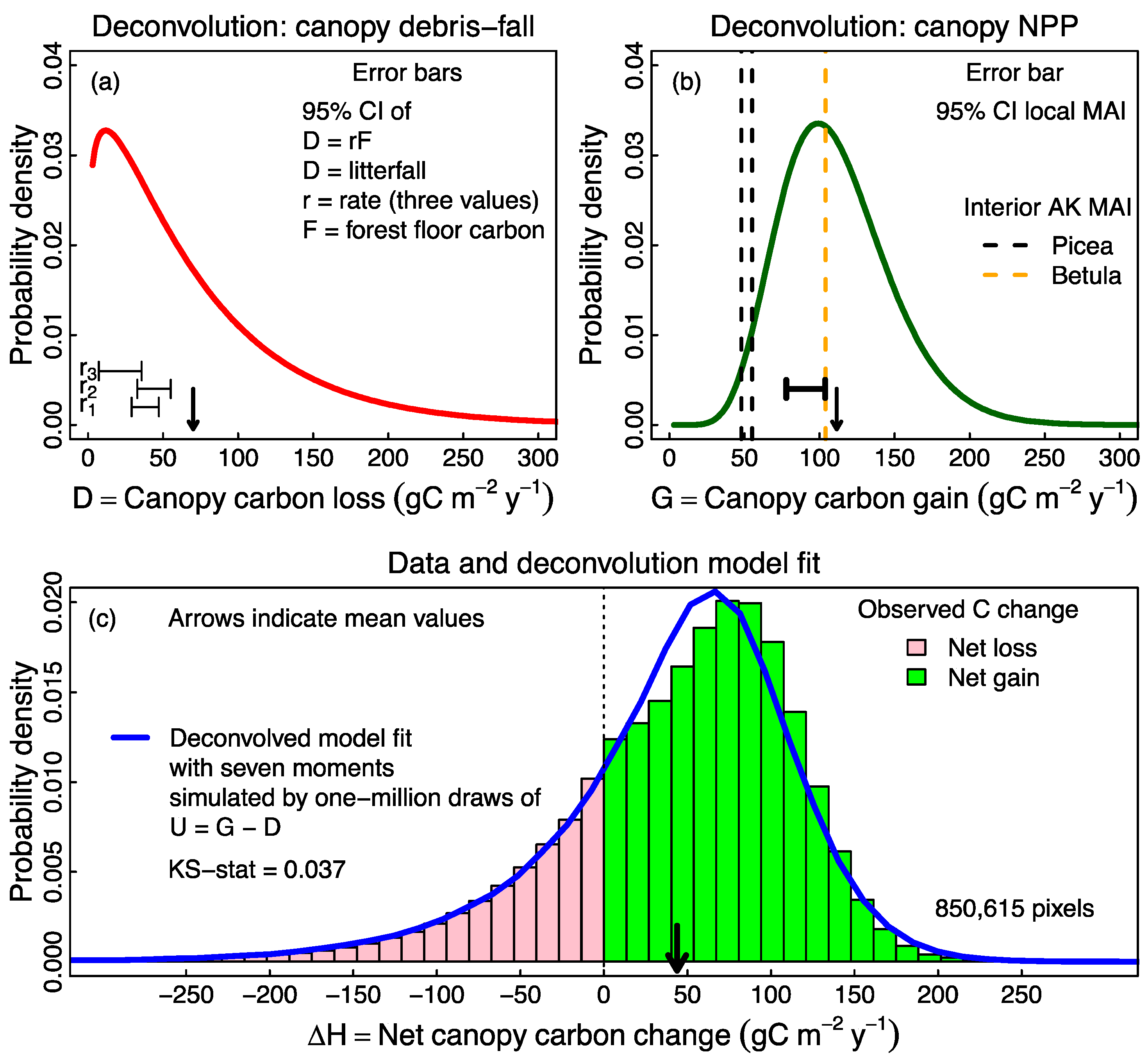
2.4. Probabilistic Deconvolution

The deconvolution model applied here treats the observed Δ H as the difference between two variables whose values are each drawn independently and randomly from gamma distributions: G representing carbon gain through canopy-level NPP, and D representing carbon loss through general debris-fall, including leaves, stems, branches, trunks, and whole trees. The model considers the observed difference in pixel-i as Δ H i = g i d i   where g i and d i are the unobserved realizations drawn from G and D repsctively for pixel-i. G and D are considered non-negative, gamma distributed random variables whose parameters (i.e., shape and scale) vary by vegetation type, canopy structure, and landscape elevation. Interpretations can be varied by investigators.
Gamma distributed variables are non-negative (X ≥ 0) whose distributions are defined by shape ( h > 0 ) and scale ( s > 0 ) parameters. The variance σ 2 = h s 2   of a gamma distribution is proportional to its mean as μ = h s . Its mode at X =   μ s is an asymmetric “hump” located left of the mean by a distance equal to the scale parameter. As shape grows larger relative to scale, the gamma approaches a normal distribution; the deconvolution here also applies to normal distributions. If a gamma distribution has scale c and shape one ( h = 1), then the distribution is exponential, with mode at X = 0, and rate parameter 1 / s > 0 . The properties of the gamma function give moments for a gamma distributed random variable X ~ Γ [ h , s ] as
E [ X n ] = h ( h + 1 ) ( h + 2 ) ( h + n 1 ) s n
where E [ · ] is the expectation operator. Assuming carbon gain G measures NPP or growth and is gamma distributed with shape parameter a and scale parameter b , symbolized as G ~ Γ [ a , b ] , then μ G = a b with σ G 2 =   a b 2 . Similarly, if carbon loss D measures litter-fall and is gamma distributed as D ~ Γ [ c , d ] , then μ D = c d and σ D 2 = c d 2 . If D is exponentially distributed, then D ~ Γ [ 1 , d ] with μ D = d and σ D 2 = d 2 .
The modeling approach assumes that for fixed values of elevation, vegetation type, and canopy structure (e.g., low elevation, Closed Mixed, 10–12 m tall forest), D is exponentially distributed because it represents primarily singular removal events (e.g., a windstorm), while G represents an accrual of incremental events (e.g., daily growth over a season). However, when combining samples from different height classes within the same vegetation type, we expect the distribution of loss rates D to include multiple exponential distributions and so apply a more general gamma distribution.
The probability density function (PDF) of the difference of two exponential distributions has a closed, analytic form of two scale parameters with a mode at zero. The PDF of the difference of two gamma distributions possesses a non-zero mode, but requires four parameters and has no closed, analytic form, hampering maximum likelihood and Bayesian methods of fit. The PDF of the difference of a gamma and an exponential random variable allows a non-zero mode with only three parameters. Here, when applying deconvolution of observed Δ H by height class within a given vegetation type, we consider the deconvolution model between gamma G and exponential D with a total of three parameters; however, when applying deconvolution across forest heights within a vegetation type, we also fit the more general difference of gamma distributions with a total of four parameters. We chose between three and four parameter models using the two-sample Kolmogorov–Smirnoff (KS) statistic comparing the observed pixel data (i.e., histograms in Figure 1) to one million draws from the best-fit gamma difference models (i.e., blue curves in Figure 1), choosing the model with the lower KS-statistic (see below).
We used the un-centered moment equations for the difference of two gamma distributions U = GD as the expectation of the nth power of U [31] in our application of GMM
E [ U n ] = k = 0 n ( n k ) ( 1 ) k E [ G n k ] E [ D k ]
with E [ G n k ] and E [ D k ] found using Equation (2). Applying Equations (2) and (3) provides the first three centered moments (mean μ U , variance σ U 2 and skewness γ U ) for estimating start conditions as:
μ U = a b c d ,   σ U 2 = a b 2 + c d 2 , γ U =   2 ( a b 3 c d 3 ) ( a b 2 c d 2 ) 3 / 2
The generalized method of moments statistically combines observed data with the information in population moment conditions to produce estimates and inferences of the unknown parameters for a given model of random variables. Here, we modeled observed Δ H as the difference between G and D or U = G D . We extracted distributions of gamma distributed carbon gain ( parameters   a and b ) and carbon loss (parameters c and d) using theorems of linear combinations of random variables and the single-step GMM with the R package gmm [13].
Prior to the GMM deconvolution of our dataset we tested the method with deconvolution of random simulated differences between gamma distributed variables with known distributions. The method worked well in recovering the known distribution parameters for large samples (n ≥ 104) but poorly for small ones (n ≤ 103).
To simplify the search for start values, we assumed that carbon loss through debris-fall was exponentially distributed with c = 1 and used the first three centered moments to find starting values of a, b, and d: Δ H ¯ =   a b   d , s d Δ H 2 = a b 2 + d 2 , s k e w Δ H = 2 ( a b 3 d 3 ) ( a b 2 d 2 ) 3 / 2 from Equation (4). These three moment equations together with R packages rootSolve [34] and moments [35] enabled solution of suitable starting parameter values for package gmm’s numerical method gmm(·). The function gmm(·) uses vector-valued functions g ( θ , Δ H i )   of differences between moment functions of unknown parameters θ and observed moments of Δ H . The differences are set equal to zero and solved numerically for the θ that best satisfies the moment conditions. For example, with m observed net changes in aboveground carbon among m pixels as Δ H i ,   i = 1 , , m ,   the function gmm(·) yields the vector of unknown parameters θ = [ a , b , c , d ] T used in G ~ Γ [ a , b ] and D ~ Γ [ c , d ] by solving the system of differences of n ≥ 4 moment functions E [ g ( θ , Δ H i ) ]
E [ g ( θ , Δ H i ) ] = E [ U ( θ )   Δ H i U 2 ( θ ) Δ H i 2   U 3 ( θ ) Δ H i 3   U n ( θ ) Δ H i n   ] = 0
where E [ U n ( θ ) ] is the nth moment of U and depends on θ from Equation (3). The summary(·) function in gmm provides parameter estimates for elements of θ and their standard errors, t-statistic and p-values.
Once θ and its standard errors describing the distributions G and D were estimated, we constructed U = G D by drawing one-million samples each from G ~ Γ [ a , b ] and D ~ Γ [ c , d ] , subtracting them, and then constructing a curve through the midpoints of a suitably binned histogram for comparison to the observed distribution of Δ H . Figure 1 shows an example using seven moment (n = 7) conditions in Equation (5). The pink and blue histogram (Figure 1c) is Δ H . The deconvolution of net carbon change Δ H into canopy carbon gain G and carbon loss D is shown in Figure 1b,c respectively. The blue curve superimposed on the histogram was constructed as 106 samples of G minus D. It shows a rather poor fit indicated by a relatively large two-sample KS-statistic (KS-stat > 0.03), a fit improved when considering landscape covariates (see Results).
We checked fits of varying moment conditions and parameter vectors using the two-sample KS-statistic. In applying the two-sample KS, the first sample was the data Δ H i ,   i = 1 , , m . The second sample was the difference between one million draws from each of the two gamma distributions described by θ and so simulating U = G D . We used the KS-statistic (often called “D” in the literature) for model selection. A smaller value of the KS-statistic indicated better agreement between observed Δ H and the deconvolution model U = G D than a larger value of the statistic. The delta method of error propagation provided standard errors of the means as s e G ¯ 2 =   a 2 s e b 2 + b 2 s e a 2 and s e D ¯ 2 =   c 2 s e d 2 + d 2 s e c 2 .
Motivated by the GAM fit of Δ H to 2002 Ht and Elev (Table S2), we investigated the deconvolution model where G and D depended on Ht of forest vegetation type-i (Vi, where i is Broadleaf, Mixed, and Needleleaf) as Δ H ( H t , V i )   ~   U ( H t , V i ) =   G ( H t , V i ) D ( H t , V i ) . For the three vegetation types we plotted G and D parameter values of Δ H against Ht to find equilibrium canopy heights where G equals D, treating D as an exponentially distributed random variable. In a second application of the deconvolution model, G and D depended on vegetation type (Vi: Broadleaf, Mixed, and Needleleaf), canopy structure (Strj: Woodland, Open, Closed), and Elevk (Low vs. High) as:
Δ H ( V i , S t r j , E l e v k ) ~ U ( V i , S t r j , E l e v k ) =   G ( V i , S t r j , E l e v k ) D ( V i , S t r j , E l e v k )
In this second model (Equation (6)), we investigated the interactions among the three factors (Vi, Strj, and Elevk) in determining G and D to determine where Δ H ¯   was similar among given combinations of factor levels, yet the latent variables G ¯ and D ¯ differed among these given combinations of factor levels. This illustrates how deconvolution of observations of net carbon change (as measured through Δ H ¯ ) can reveal complex fluxes among carbon pools. We used Equation (6) to generate parameter values for G and D among 16 combinations of factor levels: 1 structure level (Woodland) × 3 vegetation levels + 2 structure levels (Open, Closed) × 3 vegetation levels × 2 elevation factor levels + Open Mixed forest above 200 m·asl. This model considered both exponentially and gamma distributed D.

3. Results

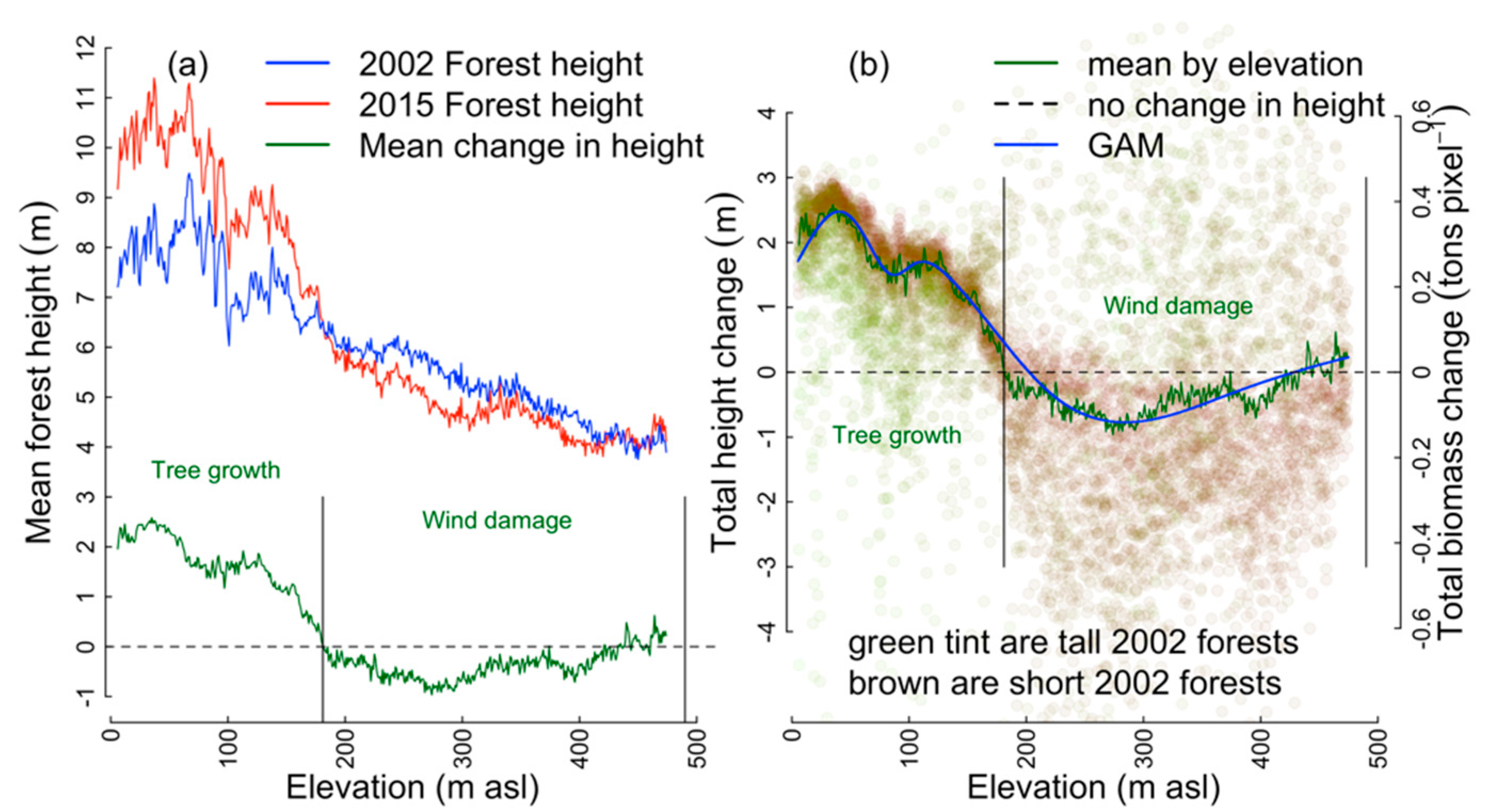
3.1. GAM Predictors of Net Change in Aboveground Tree Carbon, Δ H = U

The net canopy carbon change observed as Δ H ,   varied both by elevation and by Ht as CHM2002 pixel value (Figure 2). Below 100 m asl, Δ H was relatively constant across elevation. As elevation increased above 100 m asl, Δ H decreased rapidly, reaching a minimum near 275 m asl (Figure 2a). Above 185 m asl forest canopies averaged across 13 m pixels lost up to 1 m in height on average over the 13y period equivalent to Δ H = 32.7 gC·m−2·y−1. A single covariate GAM matched Δ H by elevation well (Figure 2b) but bivariate GAM and quadratic linear models with interactions suggested Ht, Elev, and their interaction explained over half of the variability in Δ H (Table S2). At low elevations, maximum Δ H occurred at intermediate forest height (Ht = 10–12 m). At Ht > 10–12 m, Δ H dropped steeply with increasing height. As expected in a montane forest setting, there was a general trend downward in Ht with increasing elevation (Figure 2a). By comparison, a linear model of Δ H using quadratic covariates Ht and Elev and their interactions displayed nearly identical predictions to the GAM across the study area.

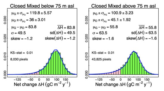
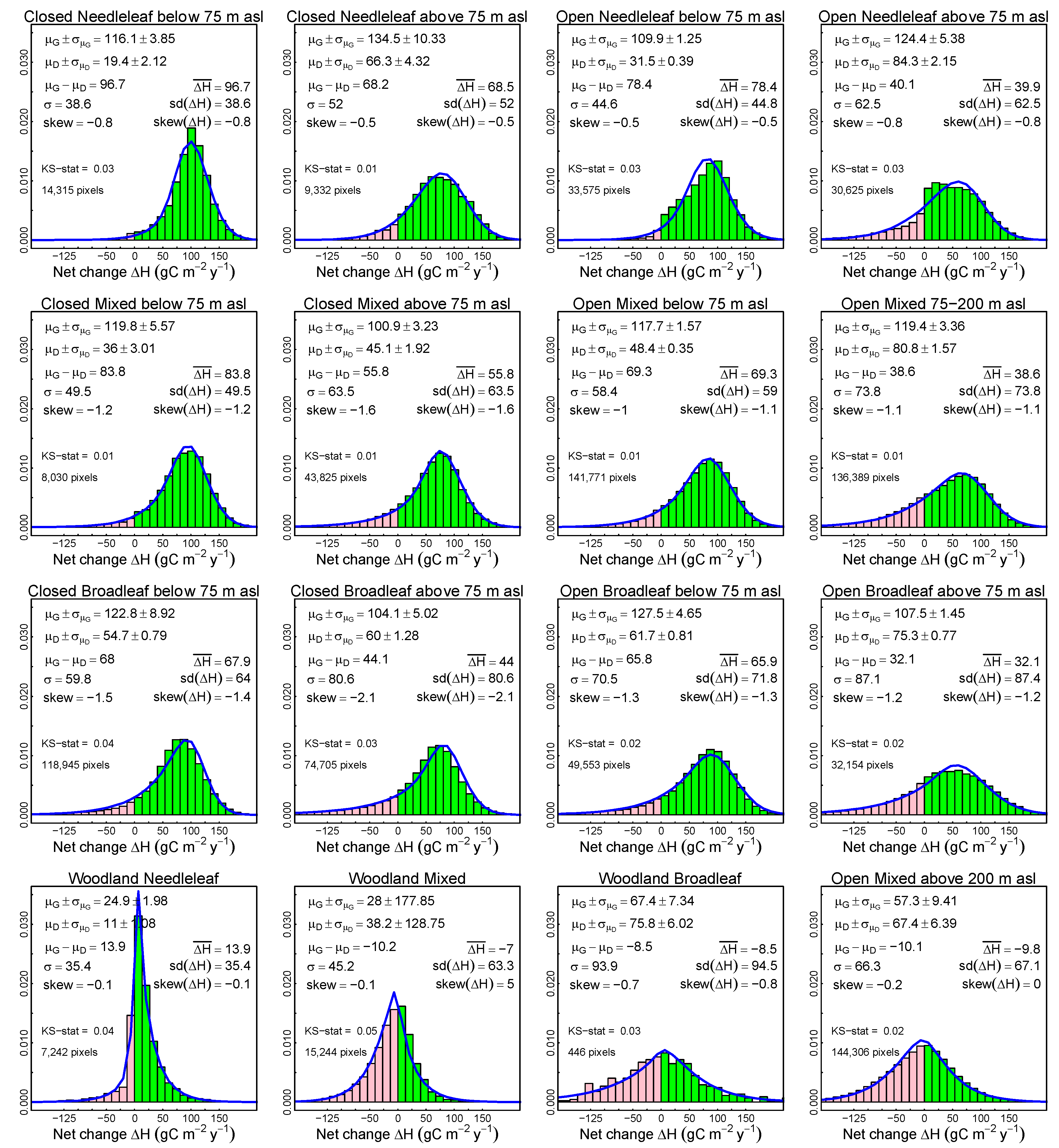
3.2. Probabilistic Deconvolution

Over all 8.5 × 10⁵ 1 m pixels (Figure 1), the distribution of Δ H was unimodal, with a mode near Δ H = 80 gC·m−2·y−1 and a mean Δ H ¯ = 40 gC·m−2·y−1. Deconvolution of Δ H with 7 moments gave a landscape-wide mean (se) carbon gain rate G ¯ =   111 (1.1) gC·m−2·y−1 and mean C loss rate D ¯ = 67 (0.6) gC·m−2·y−1, although fit was relatively poor when treating all samples as one distribution. Within forest vegetation types and across canopy heights, G ¯   varied as 95–134 gC·m−2·y−1 and D ¯ as 35–134 gC·m−2·y−1. Across the 16 combinations of structure, vegetation, and elevation factor levels, G ¯   varied as 25–134 gC·m−2·y−1 and D ¯ as 11–84 gC·m−2·y−1, showing substantial variation in both mean carbon gain through NPP and carbon loss rates through litter fall was attributable to measured covariates (Figure 3 and Figure 4).

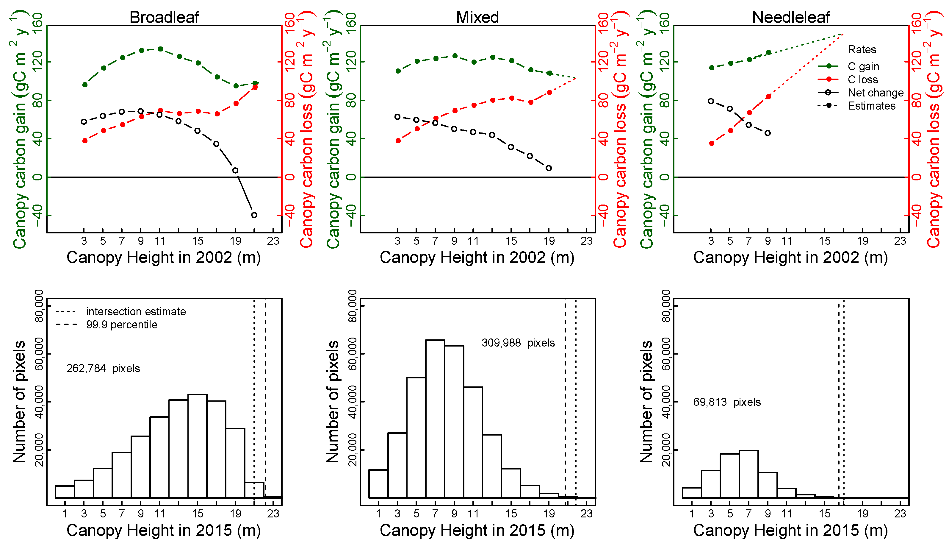
3.3. Predictors of Carbon Gain and Canopy Loss: Canopy Height and Taxonomic Composition

In Mixed and Needleleaf vegetation types Δ H , the observed value of U = GD, decreased with increasing Ht, suggesting a decrease in canopy growth increment with increasing height (Figure 3). Broadleaf showed a curvilinear response with a maximum Δ H at about 9 m, implying that only Broadleaf forest canopies increased in Δ H as Ht increased and did so only over the first third of their range in canopy height.
The deconvolution of Δ H as the difference of G ~ gamma and D ~ exponential showed that carbon gain rates, G, were maximal at intermediate height for Broadleaf (Ht = 11 m, 134 gC·m−2·y−1) and Mixed (Ht = 9 m, 126 gC·m−2·y−1) vegetation types; only Needleleaf G rate increased monotonically with height class (Figure 3). All three vegetation types increased in G monotonically below 9 m. Mixed forest showed a more constant G above 7 m than Broadleaf growth. Broadleaf G was nearly identical at 3 m canopy (96 gC·m−2·y−1) and 19 m (95 gC·m−2·y−1) heights. Carbon gain rates, D, increased with height class for all three vegetation types (Figure 3), but were relatively constant for Broadleaf forests from 11–17 m.
In each vegetation type, D increased with height more steeply than did G, consistent with an equilibrium height HtE where Δ H = 0   when D matched G (Figure 3). As the early successional forest sere in southcentral Alaska, Broadleaf was widespread across the study area and the tallest vegetation on average. Broadleaf’s 99.9 percentile CHM2015 pixel height, Ht0.999 = 22.2 m, was within 0.6 m of calculated equilibrium height (HtE = 21.6 m). Less abundant Needleleaf forest, generally a self-replacing successional sere, grew to Ht0.999 = 16.5 m, within 0.6 m of calculated equilibrium canopy height (HtE = 17.1 m). Similarly, Mixed forest, the most widespread type, grew to Ht0.999 = 20.7 m, within 1.2 m of calculated equilibrium canopy height (HtE = 21.9 m).

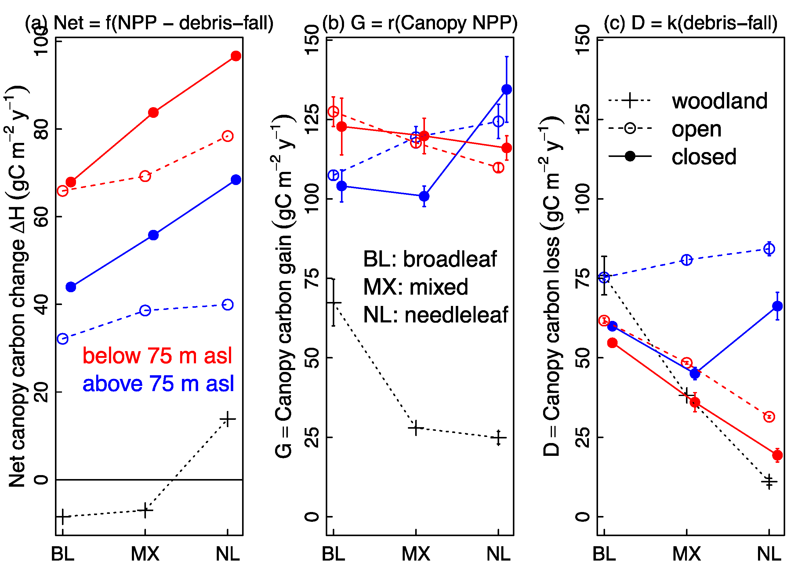
3.4. Predictors of C Gain and C Loss: Canopy Structure, Taxonomic Composition and Elevation

When parsed by vegetation type, canopy structure, and elevation factors (Figure 4), the deconvolution model fit over half the observed Δ H across the 16 combinations of the three factors very well (KS = 0.01). Seven of the 16 observed distributions of Δ H fit the difference model’s μ U , σ U , and γ U   (“centered moments”) to the first decimal place: three Needleleaf forest combinations, three Mixed combinations, and one Broadleaf. Three additional forest combinations differed in a single centered moment by at most 0.1 (two Needleleaf and a Broadleaf). The five worst fits differed in two or more centered moments by 0.1 and included the three factor combinations with all Δ H ¯ < 0 (two Woodlands and Open Mixed forest above 200 m·asl), as well as a Broadleaf and Mixed forest. Based on the first three centered moments the deconvolution model fit Needleleaf forests best and Broadleaf worst; however, the KS-statistic (Figure 4) suggested the deconvolution model fit all four Mixed forests below 200 m asl (KS = 0.01) better than other vegetation types. Eight of the 16 combinations demonstrated KS ≤ 0.02 (relatively good fits) and three combinations KS ≥ 0.04 (relatively poor fits).
Across all 16 structure-vegetation type-elevation factor combinations displayed in Figure 4, net canopy carbon change Δ H showed no evidence of interactions among factors (Figure 5a): Δ H was greater at High elevation than Low for fixed structure and vegetation type; Needleleaf Δ H was greater than Mixed and Broadleaf Δ H for fixed structure and elevation; and Closed forest Δ H was greater than Open or Woodland structure Δ H for fixed elevation and vegetation type.
In contrast, canopy NPP as G and debris-fall as D showed evidence of interactions among factors, suggesting that canopy NPP and debris-fall respond in a complex fashion to environmental conditions. A clear interaction effect was presented as elevation:vegetation type on G and D rates (Figure 5b). At Low elevation G for both Open and Closed Broadleaf was greater than for Needleleaf, while at High elevation the reverse held: G for both Open and Closed Needleleaf was greater than for Broadleaf.
Perhaps responding to the last decade of elevational-dependent warming, the highest NPP rates as G were, surprisingly, in Needleleaf High elevation forests (Closed and Open; Figure 4, top row) and Open Broadleaf Low elevation forests (Figure 4, third row, third column). Low NPP rates as G were associated with Woodland and Open Mixed forest above 200 m (Figure 4, bottom row).
Consistent with increased exposure to damaging mountain winds, the highest debris-fall rates as D rates were in Open High elevation forests of all three vegetation types (Figure 4, right column) and it was increased D rate, not reduced G rate, that led to High elevation forests of all types having the smallest Δ H (Figure 5a), again consistent with more debris-fall where wind damage was highest.
The estimates for NPP as G in Mixed forest were intermediate between Broadleaf and Needleleaf in all cases (Figure 4, top three rows) but Closed Mixed High elevation (above 75 m asl) forest where the Mixed forest G was lowest, suggesting a somewhat weak, three-way interaction among all covariates (Figure 5b). Similarly, the vegetation:elevation interaction for D presented as a greater Broadleaf Low elevation D than Needleleaf Low elevation D, yet greater Open Needleleaf High elevation D than Open Broadleaf High elevation D (Figure 5c). Among High elevation Closed forests, the weak three-way interaction was apparent where Mixed forest was again the smallest flux (Figure 5c).
The interactions described above highlight the potential difficulty of assigning carbon loss from the canopy into the forest floor brown pool without deconvolution of differenced repeat standing carbon measurements. For example, canopy carbon loss D was similar in Mixed Woodland and Mixed Closed Low elevation (i.e., 41 gC·m−2·y−1; Figure 5c), even though differences between Mixed Woodland and Closed Mixed Low elevation ∆H exceeded 102 gC·m−2·y−1 (Figure 5a). A focus on net canopy carbon change would obscure these similar rates in debris-fall.

4. Discussion

We have shown a novel application of the econometric method known as the “generalized method of moments” [12,13] to uncover strictly positive latent variables from differenced time series of lidar data (TSL) in a useful forest ecological context. Here, the differenced TSL were changes in forest carbon estimated using lidar-assisted regression. The latent variables uncovered were gamma distributed canopy carbon loss interpreted as debris-fall and canopy carbon gain interpreted as NPP. The distributions of debris-fall and NPP provided critical insight into the forest ecology under study in southcentral Alaska and were used for forest carbon accounting [36].
Forest NPP cannot be measured directly [37] and despite its importance, debris-fall is rarely fully measured at all. Field challenges have led to eddy co-variance approaches and more recently RSPs to measure NPP. The statistical technique and CRAN-available R package here are novel in the field of remote sensing as applied to TSL-assisted measurements of forest canopy carbon. The observations of net change in landscape assessments of forest canopy carbon can be considered as the difference in two, non-negative random variables, here interpreted as canopy carbon gain from forest canopy NPP minus canopy carbon loss from debris-fall. This simple model treats the two rates as independent draws from gamma distributed variables whose difference is measurable with sequential remote sensing, such as lidar and SFM. We present results of a deconvolution of serial canopy height measurements using lidar into NPP and debris-fall distributions using the generalized method of moments [12] with the second author’s package gmm [13]. Deconvolution of net change in canopy height at the landscape scale during 1.3 decades of forest dynamics in southcentral Alaska suggests that canopy level NPP and debris-fall rates covary with landscape position, canopy structure, taxonomic composition, and their interactions, results hidden in the distributions of net change alone.
Applying the method in an ecological context, we found that high elevation forests likely deposited 50–100% more biomass and carbon as debris-fall than lower elevation forests, yet canopy NPP in both high and low elevation forests were potentially within 30% of each other (canopy carbon gain: 102–135 gC·m−2·y−1) when averaged over 13 years. We estimate Woodland canopy NPP as one-half to one-fifth the rate of equivalent forest types of different structure, but with debris-fall similar to low elevation forests of similar type but differing structure. The lowest debris-fall rates were observed in low elevation Needleleaf forests and Needleleaf Woodland, suggesting that Needleleaf forest had the least debris-fall. Given the donor-pool dominated nature of C-cycling [18], if more litter flows into brown pools, then more carbon is likely available for burial in black pools, where the greatest proportion of boreal carbon is stocked. Thus, soil carbon pools in higher elevation Needleleaf forests may be growing increasingly carbon-rich relative to warmer, lower elevation Needleleaf forests pools. In lower elevation Needleleaf forests, a combination of less influx from lower rates of debris-fall and more outflux due to warmer temperatures leaves less soil carbon [38] than in higher elevation Needleleaf forests.
Canopy carbon NPP and debris-fall covaried with canopy structure measured as canopy height and canopy closure. In particular, while net change in canopy carbon decreased with increasing canopy height, NPP in mixed and broadleaf forests increased to a maximum, then decreased, while debris-fall rates in all forests increased with forest canopy height. This result is consistent with forest-stand studies showing that aboveground NPP peaks early in stand development and gradually declines by about a third [33] as size-mediated aging reduces vigor in tree above-ground NPP [3]. Here, Broadleaf forest NPP declined by 29% from a maximum where canopy height was 11 m to a minimum where canopy height was 19 m. These results motivate an additional hypothesis limiting stand height below that occurs below physiological constraints [39]: when canopy NPP equals debris-fall, as through disturbance, then net carbon accumulation in the canopy can be considered at equilibrium. This is a canopy-specific example of the well-documented ecosystem dynamic that total carbon converges to a fixed value as carbon losses come to equal inputs [18].
The novel approach of estimating NPP and debris-fall presented here is potentially informative and merits further study and application, but, like all models, suffers from several weaknesses. The most critical is the assumption of independence of draws of NPP and debris-fall. The model’s accuracy is insensitive to correlated means of NPP and debris-fall; however, simulations with correlation between the variable values chosen randomly—a violation of the independence assumption—leads to misleading results.
While we report the means of NPP and debris-fall as gC·m−2·y−1, re-measuring forests at these mass (g), spatial (m2), and temporal (y) scales would likely strongly violate independence, because small-scale growth and damage may strongly co-vary and so not be independent. Re-measurements for the estimates we present occurred at the decadal scale and were aggregated at over 150 m2. At this longer and larger spatio-temporal scale, covariance between NPP and debris-fall is likely de-coupled because longer time spans and spatial aggregation permit the stochastic nature of damage and disturbance events determining debris-fall to operate independently from favorable growth conditions affecting canopy NPP. While we have not done so, changing units to reflect the scale of measurements (e.g., kgC 102m−2·decade−1) would be a more accurate approach.
A second weakness is that while deconvolution appears to successfully disentangle the distribution of the difference of two lidar measurements as “G rate minus D rate”, calling the two variables “NPP” and “debris-fall” do not make them so. We offer three crude checks against the calculations to at least constrain their values: (1) We compare estimates of NPP rate from deconvolution to independently derived estimates from trees aged and allometrically-sized for carbon together with plot-based tree counts and (2) show that covariates increasing the probability of windthrow during the 2012 extreme wind event also increase debris-fall, but (3) find that a regional downed forest bole decay rate for log decomposition applied to field measures of downed forest debris under-predicts debris-fall from the study-site wide deconvolution.
Comparing canopy-level NPP here with other Alaskan studies. With respect to point (1) in the above paragraph, deconvolution of net carbon change gave landscape-wide mean NPP of 111 gC·m−2·y−1 and debris-fall of 67 gC·m−2·y−1. We counted 644 trees (DBH > 10 cm) among 59 field plots (Appendix A), then aged and measured 114 individual trees of three species outside the study plots providing an estimate of mean biomass accumulation increment per tree as x ¯ =   1.4 × 10³ gC·y−1·tree−1 (se = 80 gC·y−1). Multiplying trees·plot−1 by gC·y−1·tree−1, then averaging across plots gave 95% CI 78–103 gC·m−2·y−1 (Figure 1b), 7% less than the deconvolution mean NPP. Published field values for Alaskan forest NPP are scarce, but Gower et al. [33] report mean aboveground forest stand carbon divided by stand age (MAI) for Interior Alaska Picea glauca (48–55 gC·m−2·y−1) and Betula papyrifera (104 gC·m−2·y−1), suggesting that the method presented here estimates MAI when applied at the decadal scale we sampled. Gower et al. provide aboveground NPP (i.e., NPP as used here representing canopy carbon) from a three-year study of the same stands as 260–310 and 540 gC·m−2·y−1 but indicate that MAI and NPP are strongly correlated (r2 = 0.65, p < 0.01) across boreal NPP studies and recommend applying the regression of NPP on MAI as means of estimating NPP. We speculate that deconvolution at the decadal and landscape scale estimates MAI more closely than annual NPP; however, more study on the relationship between MAI and annual NPP, in general, is warranted.
Comparing covariates of debris-fall here with a fifty-year wind event. Of 11 covariates explored to predict large patches of windthrow in a logistic regression of windthrow from the 2012 wind event, the lowest AIC model included 95th percentile of CHM, elevation, and topographic position index (Appendix B). As with debris-fall, the probability of windthrow increased with elevation and canopy height (Figure S3a). Mapping windthrow probability at low elevations across the study area (Figure S3b) showed that 90% of windthrow occurred within Broadleaf, 10% within Mixed and none in Needleleaf forest, results consistent with Low elevation Broadleaf debris-fall as more than double Needleleaf debris-fall and Mixed intermediate (Figure 5c).
Regional decomposition rates back-calculated as debris-fall for comparison with estimates here. Disturbance damages and kills trees, depositing woody debris and leaf litter on the forest floor through debris-fall. Downed debris surveys across the study area (Appendix A) estimated a mean (se) density of downed debris as w ¯   = 976 (87) g·C·m−2. Yatskov [32] measured log decomposition for three phases of log decomposition (Figure 1a) on the nearby Kenai Peninsula at mean (se) exponential decay constants of 0.022 (0.003) ≤ r ¯   ≤ 0.045 (0.004) y−1. If debris-fall deposits canopy carbon at a mean annual rate D, then w(t) = De−rt remains after t years. Integrating w(t) across the life of the forest approximates the equilibrium forest floor litter as w ¯   calculated as:
lim T 0 T D ¯ exp ( r t ) d t =   D ¯ r = w ¯
with D ¯ = r w ¯ after solving Equation (6) for debris-fall D. Substituting in means and standard errors gives three 95% CI, one for each decay phase from [32], one of which gives a 95% upper limit of 55 gC·m−2·y−1, 18% less than the deconvolution mean debris-fall (Figure 1a).

5. Conclusions

This section is not mandatory but can be added to the manuscript if the discussion is unusually long or complex.

Supplementary Materials

The following are available online at https://www.mdpi.com/2072-4292/13/5/891/s1, Figure S1: Phenology from 1 April (day of year = 91) to last lidar flight for 2002 (blue) and 2015 (red), Figure S2: Lidar-assisted models of standing tree biomass equal to twice carbon, Figure S3: Windthrow following September 2012 wind event when the maximum sustained two minute wind speed at Ted Stevens Anchorage International Airport was recorded as 175 km h−1, Table S1: Best lidar-based models as predictors of aboveground standing tree carbon, Table S2: General additive models of change in canopy carbon, Δ H , from 2002 to 2015, Table S3: Correlations among independent variables used in logistic regression of 0.25 ha windthrow samples., Table S4: Model comparisons for logistic regression of 0.25 ha windthrow.

Author Contributions

Conceptualization, R.D. and H.-E.A.; methodology all authors; software, P.C.; validation, R.D., M.A., T.D., T.S.S., R.W. and T.G.; data curation, T.D.; writing—original draft preparation, R.D.; writing—review and editing, R.D., R.W.; visualization, R.D.; supervision, M.A.; project administration, R.D.; funding acquisition, R.D. and H.-E.A. All authors have read and agreed to the published version of the manuscript.

Funding

This research was funded by the 673d CES/CEIE Natural Resources Programs, U.S. Army Corps of Engineers sponsored this research in part as FXSB61518216 and USDA PNW Agreement 19-JV-11261989-112.

Institutional Review Board Statement

Not applicable as this study did not involve human or animal subjects.

Informed Consent Statement

Not applicable as this study did not involve human or animal subjects.

Data Availability Statement

Data are available on request from corresponding author.

Acknowledgments

E. Lewis-Clark, P. Bennetts, J. Walters, and M. Behler assisted in field work; B. Koenen, C. Johnson, and C. Brandt supported field work. Opinions, interpretations, conclusions and recommendations are those of the authors and are not necessarily endorsed by the United States Air Force.

Conflicts of Interest

The authors declare no conflict of interest. The funders had no role in the design of the study; in the collection, analyses, or interpretation of data; in the writing of the manuscript, or in the decision to publish the results.

Appendix A

Field work—We selected stratified random sample plots from classification of forest stands [20], then located these with submeter-GPS (Trimble, GeoXH 2008; TerraSync software). Field data collected in 2017 from 56 plots, styled after Forest Inventory and Analysis (FIA) subplots (1/24 acre = 168.6 m2) [26], provided training samples for a biomass model; 120 variable-radius plots [40] provided model validation. Each tree in sample plots was identified to species, with height (LTI, TruPulse 200; Impulse 200 LR; VD function) and DBH measured in FIA-style subplots if DBH ≥ 12.7 cm. We calculated biomass with height and DBH using southcentral AK, taxon-specific allometric equations [41,42,43,44,45]; if 2.5 cm < DBH < 12.7 cm we used [44] equations with DBH = 6.35 cm. Course woody debris (CWD) as downed-dead-trees, limbs, and branches was estimated in FIA-style subplots using point intercept methods [45]. All trees identified within a basal area factor 5 angle gauge in variable-radius plots were measured for height and DBH.
Lidar-assisted, spatial Carbon model—Most lidar-assisted models of carbon change depend on metrics of canopy height change and the assumption that forest carbon is one-half biomass. We sought a robust, lidar-assisted, simple linear regression model to estimate standing tree biomass and carbon in 13 m pixels for both 2004 and 2017. Model training used the 2017 field-measured biomass from 56 FIA-style subplots with 2015 lidar metrics as covariates; model validation used the 2017 field-measured biomass from 120 variable-radius plots. We investigated a variety of typical lidar metrics. Similarly, multiple regression increases R2 but risks over-fitting if applied outside the scope of training. Just as 2015 lidar generated values of 2017 biomass, 2002 lidar generated values of 2004 biomass using the 2017 biomass-trained model. This model application approach assumed: (1) similar phenology when lidar was acquired (Figure S2); (2) models using mean height offer similar estimators for lidar missions with differing pulse rates; (3) the model is ecologically appropriate over both decades; and (4) 2002-04 NPP and disturbance rates were similar to 2015–17.
Our preferred model simply regressed FIA-style subplot biomass against the mean of 1m CHM pixels (Figure S2) aggregated within 7.3 m buffers centered on the subplots, because the mean is unbiased by sample size, unlike order-based lidar metrics [27]. Moreover, the mean outperformed other lidar metrics we investigated (Table S1). The lidar-assisted model of aboveground carbon model for 2004 and 2017 was kgC/13m pixel = 0.5 (44 + 138Ht), where Ht is mean 1 m CHM height (m) aggregated into 13m pixels (se intercept = 199; se coefficient = 18; R2 = 0.67; n = 56). We applied the lidar-assisted model across the CHM rasters of 2002 and 2015 to estimate carbon in 2004 and 2017 as carbon rasters (Figure S4). Deconvolution of values from differencing these rasters gave NPP and litterfall rates.

Appendix B

Field Validation

We partially validated the deconvolution in three ways. First, we compared NPP to aged and measured trees. Second, we integrated our estimate of litterfall with published decomposition rates from a nearby longitudinal study of downed logs to estimate coarse woody debris (CWD) and compared it to field measurements. Lastly, we compared disturbance to an independent model of windthrow from an extreme wind event.
Growth—The deconvolution model provided an estimate of NPP in kg pixel−1y−1. To check this value, we aged and measured 122 trees from outside but near to 32 FIA-style subplots and 90 variable radius subplots, then calculated their biomass using regional, species-specific allometric equations [41,42,43,44,45,46], and divided biomass by age. Next, we found the mean biomass per year per tree by averaging over all 122 trees and multiplied this mean by the number of trees in each of the 59 FIA-style subplots (644 total trees) sampled for biomass to arrive at a NPP rate per subplot. This total subplot NPP was averaged across subplots as kg pixel−1y−1. Individuals included 62 Picea glauca, 47 Betula papyrifera, 8 Populus balsamifera, and 5 Picea mariana; no Populus tremuloides were aged.
The mean of individual tree carbon divided by tree age was 1.4 kgC y−1tree−1 (se = 0.08 kgC·y−1, n = 122 trees), a distribution well fit by a gamma distribution. Multiplying this mean carbon flux per tree by the 644 trees among 59 FIA subplots, then averaging across subplots, gave carbon accumulation of C ¯ =   15.1 kgC subplot−1y−1 (se = 1.03 kgC subplot−1y−1, n = 59). The 95% CI for annual NPP per FIA subplot based on aged tree NPP (13.5 ≤ C ¯   ≤ 17.5 kgC subplot−1y−1) included the mode of NPP (16.3 kgC pixel−1y−1), lending support to the observed biomass changes from 2004 to 2017.
Disturbance—We explored logistic regression to model the probability of observed windthrow from a severe September 2012 windstorm as a function of topographic and forest covariates. Digital orthophotos (0.5 m resolution; September-October 2012) of 8995 ha below 100 m asl from the northern portion of the study area were inspected as 0.25 ha samples (50 × 50 m) in a GIS. Of the n = 35,983 samples, we identified m = 195 where wind had visibly affected >1/3 of the trees per sample (>800 m2). We explored 11 covariates including the 2009 lidar to generate standard metrics (max, 95% height, mean, median, etc.), settling on three (Table S3) with the best model based on AIC (details in [20]).
The lowest AIC model of probability of windthrow used an additive model of elevation, canopy height, and local topographic position (Table S4). Taller forests, higher elevations and more prominent sites suffered higher probability of windthrow (Figure S3). Consistent with deconvolution of disturbance where Broadleaf forest had the greatest rate of disturbance and needleleaf had the least for fixed structure and elevation (Figure 5), 90% of windthrow > 800 m2 in area occurred within broadleaf, 10% within mixed, and none in needleleaf forest.

References

  1. Vanderwel, M.C.; Zeng, H.; Caspersen, J.P.; Kunstler, G.; Lichstein, J.W. Demographic Controls of Aboveground Forest Biomass across North America. Ecol. Lett. 2016, 19, 414–423. [Google Scholar] [CrossRef]
  2. Foster, J.R.; Finley, A.O.; D’Amato, A.W.; Bradford, J.B.; Banerjee, S. Predicting Tree Biomass Growth in the Temperate-Boreal Ecotone: Is Tree Size, Age, Competition, or Climate Response Most Important? Glob. Chang. Biol. 2016, 22, 2138–2151. [Google Scholar] [CrossRef]
  3. Mencuccini, M.; Martínez-Vilalta, J.; Vanderklein, D.; Hamid, H.A.; Korakaki, E.; Lee, S.; Michiels, B. Size-Mediated Ageing Reduces Vigour in Trees: Size Reduces Vigour in Tall Trees. Ecol. Lett. 2005, 8, 1183–1190. [Google Scholar] [CrossRef]
  4. Gower, S.T.; McMurtrie, R.E.; Murty, D. Aboveground Net Primary Production Decline with Stand Age: Potential Causes. Trends Ecol. Evol. 1996, 11, 378–382. [Google Scholar] [CrossRef]
  5. Goetz, S.; Dubayah, R. Advances in Remote Sensing Technology and Implications for Measuring and Monitoring Forest Carbon Stocks and Change. Carbon Manag. 2011, 2, 231–244. [Google Scholar] [CrossRef]
  6. McRoberts, R.E.; Næsset, E.; Gobakken, T. Estimation for Inaccessible and Non-Sampled Forest Areas Using Model-Based Inference and Remotely Sensed Auxiliary Information. Remote Sens. Environ. 2014, 154, 226–233. [Google Scholar] [CrossRef]
  7. Nasset, E.; Gobakken, T. Estimating Forest Growth Using Canopy Metrics Derived from Airborne Laser Scanner Data. Remote Sens. Environ. 2005, 96, 453–465. [Google Scholar] [CrossRef]
  8. Koenderink, J.J.; van Doorn, A.J. Affine Structure from Motion. J. Opt. Soc. Am. A 1991, 8, 377. [Google Scholar] [CrossRef]
  9. Hyyppä, J.; Hyyppä, H.; Leckie, D.; Gougeon, F.; Yu, X.; Maltamo, M. Review of Methods of Small-footprint Airborne Laser Scanning for Extracting Forest Inventory Data in Boreal Forests. Int. J. Remote Sens. 2008, 29, 1339–1366. [Google Scholar] [CrossRef]
  10. Eitel, J.U.H.; Höfle, B.; Vierling, L.A.; Abellán, A.; Asner, G.P.; Deems, J.S.; Glennie, C.L.; Joerg, P.C.; LeWinter, A.L.; Magney, T.S.; et al. Beyond 3-D: The New Spectrum of Lidar Applications for Earth and Ecological Sciences. Remote Sens. Environ. 2016, 186, 372–392. [Google Scholar] [CrossRef] [Green Version]
  11. White, J.C.; Coops, N.C.; Wulder, M.A.; Vastaranta, M.; Hilker, T.; Tompalski, P. Remote Sensing Technologies for Enhancing Forest Inventories: A Review. Can. J. Remote Sens. 2016, 42, 619–641. [Google Scholar] [CrossRef] [Green Version]
  12. Hansen, L.P. Large Sample Properties of Generalized Method of Moments Estimators. Econometrica 1982, 50, 1029. [Google Scholar] [CrossRef]
  13. Chaussé, P. Computing Generalized Method of Moments and Generalized Empirical Likelihood with R. J. Stat. Softw. 2010, 34. [Google Scholar] [CrossRef] [Green Version]
  14. Cao, L.; Coops, N.C.; Innes, J.L.; Sheppard, S.R.J.; Fu, L.; Ruan, H.; She, G. Estimation of Forest Biomass Dynamics in Subtropical Forests Using Multi-Temporal Airborne LiDAR Data. Remote Sens. Environ. 2016, 178, 158–171. [Google Scholar] [CrossRef]
  15. Knapp, N.; Huth, A.; Kugler, F.; Papathanassiou, K.; Condit, R.; Hubbell, S.; Fischer, R. Model-Assisted Estimation of Tropical Forest Biomass Change: A Comparison of Approaches. Remote Sens. 2018, 10, 731. [Google Scholar] [CrossRef] [Green Version]
  16. Zhao, K.; Suarez, J.C.; Garcia, M.; Hu, T.; Wang, C.; Londo, A. Utility of Multitemporal Lidar for Forest and Carbon Monitoring: Tree Growth, Biomass Dynamics, and Carbon Flux. Remote Sens. Environ. 2018, 204, 883–897. [Google Scholar] [CrossRef]
  17. Tompalski, P.; Coops, N.; Marshall, P.; White, J.; Wulder, M.; Bailey, T. Combining Multi-Date Airborne Laser Scanning and Digital Aerial Photogrammetric Data for Forest Growth and Yield Modelling. Remote Sens. 2018, 10, 347. [Google Scholar] [CrossRef] [Green Version]
  18. Luo, Y.; Keenan, T.F.; Smith, M. Predictability of the Terrestrial Carbon Cycle. Glob. Chang. Biol. 2015, 21, 1737–1751. [Google Scholar] [CrossRef]
  19. Jorgensen, M.T.; Roth, J.E.; Schlentner, S.F.; Pullman, E.R.; Macander, M.; Racine, C.H. An. Ecological Land Survey for Fort Richardson, Alaska; ERDC/CRREL Report TR-03-19; ABR Inc.: Fairbanks, AK, USA, 2003. [Google Scholar]
  20. Dial, R.J.; Smeltz, T.S.; Rinas, C.; Golden, T.; Barnett, K.; Walker, A.H.; Geck, J.E. Ecological, Climatic, and Land Cover Trends on Joint Base Elmendorf-Richardson, Alaska: 1950-2012; 673D Air Base Wing, Natural Resources Element, Joint Base Elmendorf-Richardson, Alaska Pacific University: Anchorage, AK, USA, 2015. [Google Scholar]
  21. Smeltz, T.S.; Dial, R.J.; Golden, T. Report on Timber Cruising across Joint Base Elmendorf-Richardson, Alaska, 2013; 673D Air Base Wing, Natural Resources Element, Joint Base Elmendorf-Richardson, Alaska Pacific University: Anchorage, AK, USA, 2015. [Google Scholar]
  22. Smeltz, T.S.; Rinas, C.; Golden, T.; Barnett, K.; Dial, R.J. Long-term Vegetation Monitoring on Joint Base Elmendorf-Richardson, Alaska, 2013. A Survey of Vegetation, Birds, and Small Mammals; 673D Air Base Wing, Natural Resources Element, Joint Base Elmendorf-Richardson, Alaska Pacific University: Anchorage, AK, USA, 2014. [Google Scholar]
  23. Nowacki, G.J.; Spencer, P.; Fleming, M.; Brock, T.; Jorgenson, T. Unified Ecoregions of Alaska: 2001; (No. 2002-297); Geological Survey, 2003. [Google Scholar]
  24. Berg, E.E.; David Henry, J.; Fastie, C.L.; De Volder, A.D.; Matsuoka, S.M. Spruce Beetle Outbreaks on the Kenai Peninsula, Alaska, and Kluane National Park and Reserve, Yukon Territory: Relationship to Summer Temperatures and Regional Differences in Disturbance Regimes. For. Ecol. Manag. 2006, 227, 219–232. [Google Scholar] [CrossRef]
  25. Berg, E.E.; Anderson, R.S. Fire History of White and Lutz Spruce Forests on the Kenai Peninsula, Alaska, over the Last Two Millennia as Determined from Soil Charcoal. For. Ecol. Manag. 2006, 227, 275–283. [Google Scholar] [CrossRef]
  26. Bechtold, W.A.; Scott, C.T. The Forest Inventory and Analysis Plot Design.; Gen. Tech. Rep. SRS-80; U.S. Department of Agriculture, Forest Service, Southern Research Station: Asheville, NC, USA, 2005; pp. 37–52. [Google Scholar]
  27. Harter, H.L. Order Statistics and Their Use in Testing and Estimation; US Government Printing Office: Washington, DC, USA, 1970; Volume II. [Google Scholar]
  28. Magnussen, S.; Næsset, E.; Gobakken, T. LiDAR-Supported Estimation of Change in Forest Biomass with Time-Invariant Regression Models. Can. J. For. Res. 2015, 45, 1514–1523. [Google Scholar] [CrossRef]
  29. Luo, S.; Chen, J.M.; Wang, C.; Xi, X.; Zeng, H.; Peng, D.; Li, D. Effects of LiDAR Point Density, Sampling Size and Height Threshold on Estimation Accuracy of Crop Biophysical Parameters. Opt. Express 2016, 24, 11578. [Google Scholar] [CrossRef]
  30. Wood, S.N. Generalized Additive Models: An. Introduction with R., 2nd ed.; Chapman & Hall/CRC: Boca Raton, FL, USA, 2017; ISBN 978-1-4987-2833-1. [Google Scholar]
  31. Klar, B. 31_ A Note on Gamma Difference Distributions. J. Stat. Comput. Simul. 2015, 85, 3708–3715. [Google Scholar] [CrossRef]
  32. Yatskov, M.A. The Impact of litterfall on C Stores and Dynamics in Forests of Coastal Alaska. Ph.D. Dissertation, Oregon State University, Corvalis, OR, USA, 2016. [Google Scholar]
  33. Gower, S.T.; Krankina, O.; Olson, R.J.; Apps, M.; Linder, S.; Wang, C. Net Primary Production and C Allocation Patterns of Boreal Forest Ecosystems. Ecol. Appl. 2001, 11, 1395–1411. [Google Scholar] [CrossRef]
  34. Soetaert, K.; Herman, P.M.J. A Practical Guide to Ecological Modelling; Springer: Dordrecht, The Netherlands, 2009; ISBN 978-1-4020-8623-6. [Google Scholar]
  35. Komsta, L.; Novomestky, F. Moments, Cumulants, Skewness, Kurtosis and Related Tests, R package version 0.14; 2015. [Google Scholar]
  36. Dial, R.J.; Allgeier, M.; Lewis-Clark, E.; Day, T. Joint Base Elmendorf-Richardson Forest Carbon Stock Inventory: Past, Present, and Future (FXSB61518216); 673D Air Base Wing, Natural Resources Element, Joint Base Elmendorf-Richardson, Alaska Pacific University: Anchorage, AK, USA, 2018. [Google Scholar]
  37. Clark, D.A.; Brown, S.; Kicklighter, D.W.; Chambers, J.Q.; Thomlinson, J.R.; Ni, J. Measuring Net Primary Production in Forests: Concepts and Field Methods. Ecol. Appl. 2001, 11, 356–370. [Google Scholar] [CrossRef]
  38. Knorr, W.; Prentice, I.C.; House, J.I.; Holland, E.A. Long-Term Sensitivity of Soil Carbon Turnover to Warming. Nature 2005, 433, 298–301. [Google Scholar] [CrossRef]
  39. Koch, G.W.; Sillett, S.C.; Jennings, G.M.; Davis, S.D. The Limits to Tree Height. Nature 2004, 428, 851–854. [Google Scholar] [CrossRef]
  40. Avery, T.E.; Burkhart, H.E. Forest Measurements, 5th ed.; McGraw-Hill: New York, NY, USA, 2002. [Google Scholar]
  41. Raile, G.K. Estimating Stump Volume; Res. Pap. NC-224; U.S. Department of Agriculture, Forest Service, North Central Forest Experiment Station: St. Paul, MN, USA, 1982. [Google Scholar]
  42. Larson, F.R.; Winterberger, K.C. Tables and Equations for Estimating Volumes of Trees in the Susitna River Basin, Alaska; US Forest Service Research Note PNW: Portland, OR, USA, 1988. [Google Scholar]
  43. Jenkins, J.C.; Chojnacky, D.C.; Heath, L.S.; Birdsey, R. A National scale biomass estimators for United States tree species. Forest Sci. 2003, 49, 12–35. [Google Scholar]
  44. Jenkins, J.C.; Chojnacky, D.C.; Heath, L.S.; Birdsey, R.A. Comprehensive Database of Diameter-Based Biomass Regressions for North. American Tree Species. Gen. Tech. 15 Rep. NE-319; U.S. Department of Agriculture, Forest Service, Northeastern Research Station: Newtown Square, PA, USA, 2004. [Google Scholar]
  45. Woodall, C.W.; Monleon, V.J. Sampling, Estimation, and Analysis Procedures for the Down Woody Materials Indicator; USDA Forest Service General Technical Report NRS-22; Northern Research Station: Newtown Square, PA, USA, 2008. [Google Scholar]
  46. Woodall, C.W.; Heath, L.S.; Domke, G.M.; Nichols, M.C. Methods and Equations for Estimating Aboveground Volume, Biomass, and C for Trees in the U.S. Forest Inventory, 2010; General Technical Report NRS-88; 2011. [Google Scholar]
Figure 1. Deconvolution of observed average net change in canopy carbon as unobserved canopy carbon loss (carbon loss through debris-fall) and unobserved canopy carbon gain (carbon gain through above ground Net Primary Productivity; NPP) with a 7-moment fit of their difference (blue distribution) superimposed on the histogram of observed net change in canopy carbon from lidar-assisted carbon model. The fit is poor as expected because the landscape is heterogeneous. (a) Gamma distribution of D interpreted as canopy carbon loss. Error bars show 95% CI of independent estimates of canopy carbon loss using measured decomposition rates of logs in three decay phases (r1: under 30% decomposed, r2: 30-70% decomposed, r3: 70% or more decomposed) [32] and measured coarse woody debris plus litter on the forest floor of the study area. (b) Gamma distribution of G interpreted as canopy carbon gain. Vertical lines give mean annual increment (MAI = stand biomass/stand age) for three Interior Alaska boreal forest sites [33]. Error bar gives 95% CI for MAI = mean [tree biomass/tree age]*(number of trees/plot) averaged over n = 59 plots in the study area. (c) Observed histogram of all pixels giving differences in carbon between two lidar estimates of biomass separated by 13 years with best deconvolved model fit as difference in distributions given in (a) and (b). Pink boxes tally observed pixels with net canopy carbon loss; green boxes tally pixels with net canopy carbon gain. KS-stat = Kolmogrov Smirnoff statistic as described in text indicating a rather poor fit, visible in the figure.
Remotesensing 13 00891 g001
Figure 2. Standing tree height changes from 2002 to 2015 as indicated by differenced canopy height models (13m pixel CHMs). (a) Mean forest height in 13m pixels by elevation in 2002 (blue) and 2015 (red) and their difference (Height change, green, with axis shared with Mean forest height). (b) Total eight change from 2002 to 2015 by elevation and 2002 height. Total biomass change refers to change over 13 years. Tint of points shows mean forest height in 2002 with taller and shorter canopy heights tinted green and brown, respectively. Each point represents a 2002 height by elevation bin with change in height averaged across all pixels in the bin. Blue curve is simple GAM of Δ H   ~ s(Elevation), where s(·) is the GAM smoother.
Remotesensing 13 00891 g002
Figure 3. Relationship between canopy height in 2002 and net change in canopy carbon and its deconvolution as carbon gain through aboveground tree NPP and carbon loss through debris-fall. Bullets give mean values of distributions binned by 2 m canopy height class. Lower panels show distributions of 2015 canopy heights by vegetation type. Dotted lines in top and bottom panels indicate equilibrium heights as local linearized estimates of carbon gain equals carbon loss with net carbon change equal zero, at canopy height equilibrium. Vertical dashed lines in lower panels indicate 99.9 percentile for 2015 canopy heights by vegetation type. Net change in top panels has units of carbon gain and carbon loss. For all three forest types, the expected equilibrium height based on difference between latent variables G and D deconvolved using the generalized method of moments was similar to the maximum canopy heights measured.
Remotesensing 13 00891 g003
Figure 4. Histograms of observed distributions of net canopy carbon change Δ H (green positive, pink negative) with superimposed best fit convolution (blue curve). μ G , μ D , σ μ G , σ μ D , μ G μ D give means ± standard error of means, and difference of means for canopy NPP = G and canopy debris-fall = D, respectively, with descriptive statistics for Δ H printed opposite the corresponding descriptive statistics for U = G D from deconvolution so as to make model vs. observation comparison clear. KS-stat is the Kolmogorov–Smirnov test statistic often referred to as “D” in the literature. Pixel count gives sample size in histogram.
Remotesensing 13 00891 g004
Figure 5. Interaction plots of canopy C flux by forest type, structure, and elevation. (a) Net canopy C change Δ H . (b) Canopy carbon gain and (c) canopy carbon loss. Color gives elevation, point and line type give structure. Error bars on carbon gain and loss calculated from deconvolution standard errors and delta method.
Remotesensing 13 00891 g005
Publisher’s Note: MDPI stays neutral with regard to jurisdictional claims in published maps and institutional affiliations.

