1. Introduction
Soil salinization is a major land-degradation problem in arid and semi-arid environments [
1,
2,
3,
4]. Mapping techniques that can be used to inventory and monitor soil salinization over large areas in more efficient, time-effective and less expensive ways are required for precision agriculture and sustaining soil productivity in many parts of the world. Predictive mapping techniques, such as linear and multiple regression, geostatistics (
i.e., Kriging and CoKriging), fuzzy logic, neural network, and classification and regression trees [
5,
6,
7,
8,
9] have been used to develop soil and natural resource maps. Each of these techniques provides optimal results under certain circumstances. Geostatistics, for example, yield significant results when data are normally distributed and stationary (mean and variance do not vary significantly in space); where significant deviations from normality and stationarity arise, the analysis becomes problematic [
10,
11]. This normality issue is difficult to constrain at smaller scales, especially when values of environmental parameters and soil properties dramatically change from one location to another across the soilscape. It is just such a case in mapping soil salinity, where electrical conductivity (EC) values change significantly between salt-affected and normal soils over relatively short distances within large areas. Using geostatistics in this case will result in significant errors and the predicted values will depart significantly from the original. Mapping salt-affected soils in the field is difficult as they are interspersed with normal soils and form no contiguous pattern [
12].
Geostatistical techniques such as cokriging could benefit from the availability of secondary data in developing prediction maps, but all of the data have to be numerical and normally distributed, not nominal or categorical data. Thus, valuable data such as geology and vegetation which either have a significant influence on salt accumulation or influenced by soil salinity, could not be used in producing predictive soil maps. This issue is in addition to the requirement of geostatistical techniques to large amounts of field data in order to obtain optimal results.
Decision-tree analysis (DTA), on the other hand, is a predictive mapping technique that can be used in developing soil salinity maps over large areas. It is a non-parametric or distribution-free statistical method, which means data are not required to fit a normal distribution curve. It can be used with ordinal as well as categorical attributes. Moreover, it requires no assumptions about the data and provides interpretable prediction rules that can be extrapolated to similar areas [
6,
13,
14].
Remote-sensing data have been used successfully in mapping soil salinity for decades [
2,
3,
12,
15,
16,
17,
18,
19,
20]. The principle behind this success is based on the dramatic effects that soil salinity has on soil physical, chemical and biological properties. The quantities and changes in soil properties can be monitored using remote sensing.
The objectives of this study are to demonstrate a combined method involving remote sensing data and DTA in developing soil salinity maps in an efficient and timely manner. This study was conducted in support of an initial soil survey of Malheur County, Oregon, the largest unmapped area in the USA. Recognizing the fine distinctions between five soil salinity classes used by the US Department of Agriculture Natural Resources Conservation Service [
21] is one of the means by which soil map units are being designed and delineated in the survey area.
2. Materials and Methods
2.1. Site Description
Field reconnaissance of the study area, located in central Malheur County, southeastern Oregon, USA (
Figure 1), reveals that saline soils and intergrades are abundant. For this experiment, a 1,160 km
2 area was chosen, covering the range of saline soils thought present in the region [
22]. Surface elevation ranges from 1,175 to 1,771 m (mean = 1,297 m) aMSL and slopes range between 0 to 57° (mean = 2°). Aridisols are the dominant soil order [
23] in the area as the soil moisture regime is aridic with mean annual precipitation (MAP) varying from 178 mm in low areas to 330 mm on high elevations (mean = 254 mm); a portion of this falls as snow during winter, with 220 mm at median elevations. Soil temperature regime is mesic to frigid, with surface air temperatures ranging from monthly mean low temperature of −8° (January) to monthly mean maximum 33 °C (August).
Figure 1.
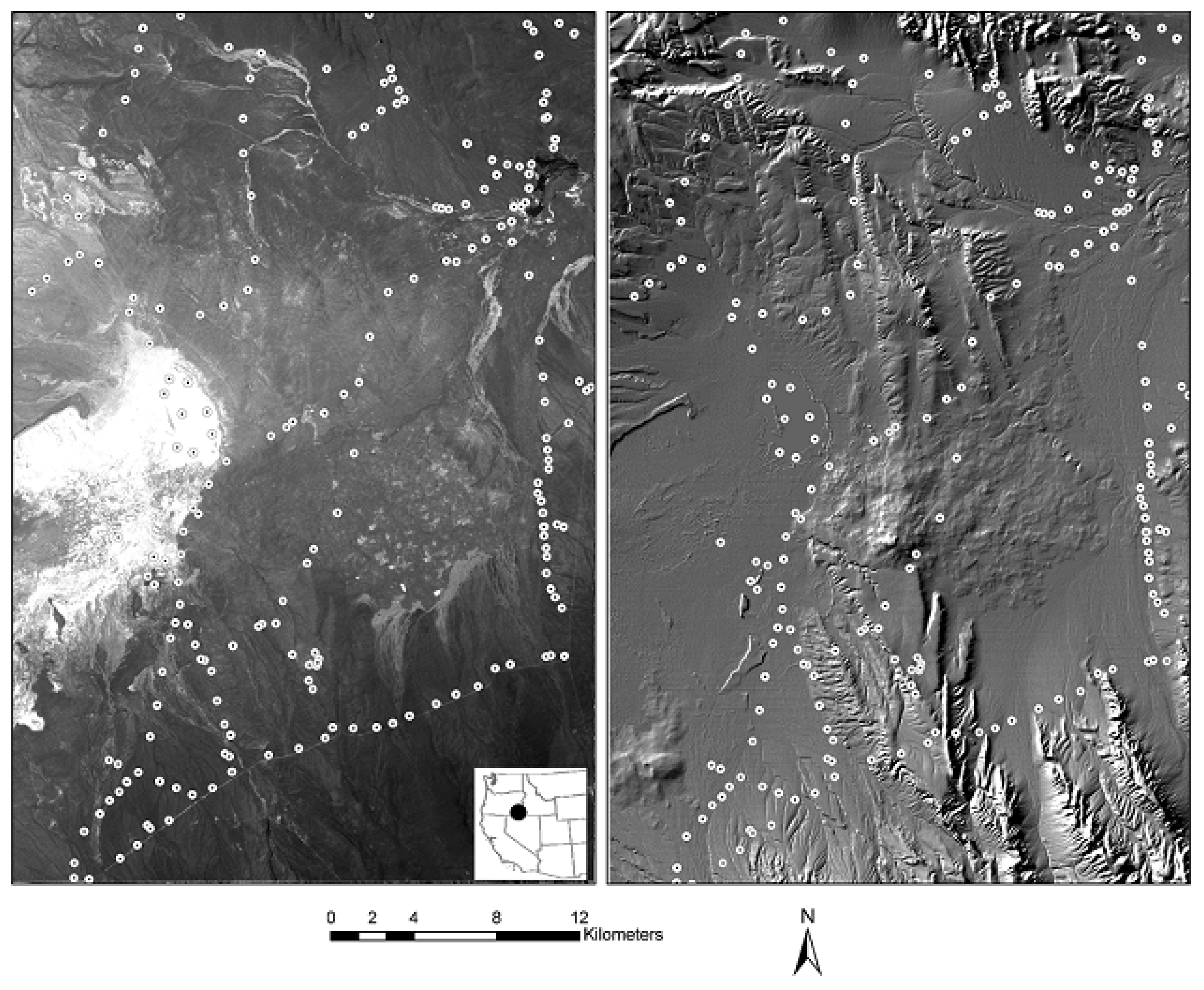
Study area, in Malheur County, southeastern Oregon, USA (see inset map), represented by a Landsat TM image of study area (left) and IFSAR DEM with hillshade (right). Both images have the overlay of soil pits and sampling points.
Figure 1.
Study area, in Malheur County, southeastern Oregon, USA (see inset map), represented by a Landsat TM image of study area (left) and IFSAR DEM with hillshade (right). Both images have the overlay of soil pits and sampling points.
Soils in the area are developed on Tertiary basalt and andesite, tuffaceous sedimentary rocks, lacustrine deposits and fluvial sedimentary rocks [
24]. Prevalent landforms in the area are alluvial fans, fan remnants, basins, flood plains, pediments, and playas. Vegetation varies from native vegetation to agricultural pasture land [
25]. Dominant native types of vegetation in the area are Wyoming big sagebrush (
Artemisia tridentata wyomingensis), Shadscale saltbush (
Atriplex confertifolia), greasewood (
Sarcobatus vermiculatus), black sagebrush (
Artemisia nova), basin big sagebrush (
Artemisia tridentata tridentata), and low sagebrush (
Artemisia arbuscula arbuscula).
Most soils in the area are well drained and depth to the water table is far away from the soil surface except for areas close to agricultural pasture land and the internal playas. Agricultural lands are pump-irrigated and irrigation water flows to nearby low-lying areas, resulting in higher water tables. Coyote Lake, in addition to many smaller playas, is an internal-draining playa (alkali flats or sabkha) that is periodically water-logged during the winter and spring seasons, and dries out during the summer. Playas are bare and shallow depressions with a high content of soluble salts and high alkalinity.
2.2. Data Sources and Description
Spatially extensive, digital data appropriate to describing the morphology and distribution of soils
cf. [
7], especially the abundance of salinity, were used in this work including: digital elevation model (DEM) data, Landsat imagery, geology, vegetation, and climate (
Figure 1). Description of the data layers and their sources is presented in
Table 1 and a more detailed description of the attribute-values for each layer is provided in
Table 2. No soil map exists for the area. Spatial data were represented using the raster data model in ArcGIS which is helpful in data modeling and data manipulation. Data layers were resized to have a spatial resolution of 30 m, which represent most of the data used in this study. To reduce errors due to georeferencing, as many of the layers are digitized from paper maps, all layers were closely examined for spatial correspondence to late-generation; USGS digital orthoquad maps (combined aerial imagery and topographic data).
Table 1.
Databases and their sources.
Table 1.
Databases and their sources.
| Variables | Data source | Scale | Type |
|---|
| Landsat TM (7 bands) | [26] | 30 m | Raster |
| Normalized Difference Vegetation Index (NDVI) | Landsat, method of [27] | 30 m | Raster |
| Soil Adjusted Vegetation Index (SAVI) | Landsat, method of [28] | 30 m | Raster |
| Normalized Difference Salinity Index (NDSI) | Landsat, method of [2] | 30 m | Raster |
| Brightness, Greenness, and Wetness | Landsat, method of [29] | 30 m | Raster |
| Band ratios b3/b1 and b5/b7 | Landsat | 30 m | Raster |
| Terrain attributes | IFSAR data (this study) | 5 m | Raster |
| Surficial geology | This study | 1:24,000 | Vector |
| Landfire vegetation | [30] | 30 m | Raster |
| Mean annual precipitation | [31] | 1:200,000 | Vector |
| Distance from streams | Multi-ring buffer in GIS | 1:24,000 | Vector |
| Ecological habitat | [24] | 1:250,000 | Vector |
Table 2.
Environmental variables and their properties.
Table 2.
Environmental variables and their properties.
| Variable | Type | Classes | Value range |
|---|
| Landsat TM bands | Continuous | Continuous | 0–255 |
| NDVI | Continuous | Continuous | 0–100 |
| SAVI | Continuous | Continuous | 0–100 |
Brightness Greenness
Wetness | Continuous
Continuous
Continuous | Continuous
Continuous
Continuous | 42–462
−60–112
−96–53 |
Elevation
Slope gradient
Slope aspect | Continuous
Continuous
Continuous | Continuous
Continuous
Continuous | 1,175–1,771
0–57
−1–360 |
| Landform | Discrete | 10 classes | 1–10 |
| Geology | Discrete | 9 classes | 101–111 |
| Historic vegetation | Discrete | 10 classes | Wide range (1–45) |
| Landfire vegetation | Discrete | 26 classes | Wide range (1–2,227) |
| Precipitation | Discrete | 4 classes | 7, 9, 11 and 13 |
| *Distance from streams | Discrete | 1 classes | 1–7 |
| Habitat | Discrete | 6 classes | 1–6 |
Elevation, terrain attributes and landforms were developed based on two digital elevation models (DEM). Initially, we used stock USGS DEMs with their 10 m grid size, but found that playa rims, dune fields and other landforms were not present or poorly resolved using such data. To improve on this we had Interferometric Synthetic Aperture Radar (IFSAR, aka InSAR) data acquired from fixed-wing aircraft and processed by Intermap Technologies, Inc. (Englewood, CO, USA), under contract with the USDA-NRCS, for our use in developing the DTA technique in its application to digital soil mapping. Because the existing (bedrock) geological map for the area is a preliminary 1:500,000 scale representation [
32] and therefore unsuitable for use in this experiment, we developed a 1:24,000-scale surficial geology map based on field reconnaissance, aerial photographs, IFSAR DEM, and the bedrock geology. The surficial geological units include age, process and material properties, e.g., Holocene aeolian sand dunes, Late Pleistocene sandy gravelly alluvial fans, and residuum on Tertiary andesitic basalt.
2.3. Soil Samples and Analysis
About 210 surface soil samples, nominally the 0–15 cm layer, were collected from soil pits excavated and described according to US Soil Survey standards [
21]. Field work occurred during the months of July and August (dry season) 2006, when salt efflorescence reaches its maximum in this region (M. Keller, personal comm., 2006). Sampling sites were selected using a stratified random sampling method modified by access concerns with existing remote dirt road network. Stratification of the random sample depended on landscape complexity and the need to represent all area-class map units [
3,
33]. Samples were air dried, crushed and sieved to pass through a 2 mm sieve.
Table 3.
Soil samples and their XY coordinates, saturation percentage (SP), field capacity (FC), pH and EC values.
Table 3.
Soil samples and their XY coordinates, saturation percentage (SP), field capacity (FC), pH and EC values.
| Sample No | Northing
(Y) | Easting
(X) | SP
(%) | FC
(%) |
pH | EC
(uS/m) | EC
(dS/m) |
|---|
| 1 | 4,732,683.5 | 427,377.94 | 23 | 11.5 | 8.61 | 520 | 0.52 |
| 2 | 4,732,738.4 | 427,408.01 | 22 | 11 | 7.95 | 440 | 0.44 |
| 3 | 4,733,171.7 | 425,123.02 | 23 | 11.5 | 7.7 | 420 | 0.42 |
| 4 | 4,729,825.9 | 426,066.03 | 22 | 11 | 6.5 | 430 | 0.43 |
| 5 | 4,729,396.5 | 425,888.5 | 20 | 10 | 7.28 | 490 | 0.49 |
| 6 | 4,727,613.1 | 426,422.18 | 17 | 8.5 | 7.38 | 360 | 0.36 |
| 8 | 4,726,609.6 | 423,415.2 | 20 | 10 | 7.3 | 580 | 0.58 |
| 9 | 4,702,650.1 | 426,927.68 | 14.6 | 7.3 | 7.29 | 630 | 0.63 |
| 10 | 4,702,676.5 | 426,253.98 | 21.78 | 10.89 | 7.04 | 700 | 0.7 |
| 11 | 4,702,615.3 | 426,017.04 | 20.76 | 10.38 | 6.68 | 290 | 0.29 |
| 12 | 4,702,239.8 | 424,288.7 | 30.08 | 15.04 | 8.24 | 670 | 0.67 |
| 13 | 4,702,049.6 | 423,567 | 27.44 | 13.72 | 8.22 | 750 | 0.75 |
| 14 | 4,700,790.2 | 421,671.78 | 19.34 | 9.67 | 7.24 | 370 | 0.37 |
| 15 | 4,699,755.5 | 419,418.24 | 21.51 | 10.75 | 6.72 | 260 | 0.26 |
| 16 | 4,699,396.5 | 418,614.62 | 25 | 12.5 | 6.5 | 590 | 0.59 |
| 17 | 4,699,157.9 | 416,709.02 | 24.8 | 12.4 | 6.65 | 180 | 0.18 |
| 18 | 4,699,196.4 | 415,714.33 | 31.13 | 15.56 | 7.64 | 590 | 0.59 |
| 19 | 4,701,045 | 414,747.16 | 24 | 12 | 7.32 | 460 | 0.46 |
| 20 | 4,701,464.7 | 414,546.51 | 24 | 12 | 7.32 | 490 | 0.49 |
| 21 | 4,698,688.2 | 415,354.86 | 23 | 11.5 | 7.5 | 450 | 0.45 |
| 22 | 4,698,174.9 | 414,068.77 | 23 | 11.5 | 7.37 | 530 | 0.53 |
| 23 | 4,697,856.8 | 412,616.4 | 24 | 12 | 7.47 | 290 | 0.29 |
| 24 | 4,697,052.9 | 410,844.16 | 23 | 11.5 | 7.61 | 1,170 | 1.17 |
| 25 | 4,697,923.7 | 410,501.52 | 21 | 10.5 | 7.44 | 480 | 0.48 |
Electrical Conductivity (EC) was measured in the soil-saturation extract in decisiemens per meter (dSm
−1) according to [
34] (
Table 3). Soil reaction (pH) was also measured in the soil paste. No data were available about water table depth and water salinity content for this remote area.
2.4. Mapping Methods
Two methods were used in this paper to develop soil salinity maps: remote-sensing analyses without and with DTA. Two Landsat TM images, acquired on August 17, 2005 [
26], were mosaiked and subsetted to cover the area of interest (
Figure 1). Salt-affected soils are usually poorly vegetated areas and stressed vegetation could be used as indirect sign for the presence of salinity. Two vegetation indices were therefore integrated in the analysis: Normalized Vegetation Index (NDVI) [
27] and Soil Adjusted Vegetation Index (SAVI) [
28]. Tassel Cap Transformation (TCT) indices (brightness, greenness, and wetness [
29] were used to distinguish areas with high spectral reflectance, green vegetated areas and soil and vegetation moisture. Band ratios such as b3/b1 and b5/b7 also were calculated and used to interpret some properties conventionally associated with non-saline soils. Band Ratio b3/b1 is found to reflect iron content as reported by [
35], whereas b5/b7 is found to have a strong correlation with clay mineral content in poorly vegetated areas [
36].
Using DTA, several additional environmental variables were incorporated in developing soil-salinity prediction maps. DTA was carried out using the See5/C4.5 algorithm [
37], a system for automated knowledge acquisition for artificial intelligence (AI) applications [
38]. A constructed decision tree consists of nodes representing variables or attributes, branches representing attribute values, and leaves representing classes. A decision tree is built based on selecting the attribute that minimizes the amount of disorder in the sub-tree rooted at a given node.
Soil samples were classified according their EC values into five classes [
21]: (1) EC < 2 dSm
−1 very low; (2) EC from 2 to 4 dSm
−1 low; (3) EC from 4 to 8 dSm
−1 moderate; (4) EC from 8 to 16 dSm
−1 high; and (5) EC > 16 dSm
−1 very high. Sampling points were buffered using a 300 m (10 pixels) buffering distance on the GIS map to collect other localized environmental data that have the major influence in developing soil salinity at each sampling location to be used in training the prediction model. These locations were randomly sampled using the Classification and Regression Tree (CART) model [
39]. About 21,400 training samples (pixels) were used to train the model, whereas about 7,600 validating samples (pixels) were used to validate the model. Training and validation data were boosted using 10 trials to enhance the prediction accuracy. Using this function results in creating a sequence of decision trees, where each subsequent tree attempts to fix the misclassification errors in the previous one. Each decision tree makes a prediction and the final prediction is a weighted vote of the predictions of all trees [
40]. Also, the growing tree was pruned by 30% to reduce the over-fitting problem and increase the model efficiency [
3].
Table 4.
Correlation between EC values and numerical environmental variables.
Table 4.
Correlation between EC values and numerical environmental variables.
| Variable | Correlation Coefficient |
|---|
| Elevation | −0.1805 * |
| Slope | −0.1378 ns |
| Band1 | 0.2498 ** |
| Band2 | 0.2902 ** |
| Band3 | 0.2562 ** |
| Band4 | 0.3837 ** |
| Band5 | 0.1283 ns |
| Band7 | 0.0581 ns |
| NDVI | −0.1445 ns |
| NDSI | 0.1445 ns |
| SAVI | −0.1328 ns |
| Brightness | 0.2570 ** |
| Greenness | −0.0590 ns |
| Wetness | 0.4537 ** |
3. Results
3.1. Field Observations
Across the area we find a significant correlation between EC values and surface elevation (
Table 4). Field observations in the study area indicate the presence of salt accumulation in low-lying landforms across the landscape, including Holocene floodplains, Holocene playas and Quaternary fluvial fans. Salts effloresced on the soil surface in the floodplain of Crooked Creek (close to the agriculture land). EC values were very high at that location and varied from 12.5 to 82.8 dSm
−1. This high salt content is associated salt-tolerant vegetation (halophytes) such as salt grass (
Distichlis spicata var. stricta.) and greasewood. Also, this location represents a low-level area and the ground water table was encountered at about 60 cm. Higher salt content was also observed in the playas—no vegetation is growing in these areas, soils are strongly compacted, and pH values are greater than 8.5. However, the salt accumulation on playa surfaces is significantly less than that observed on floodplains in the northeastern quarter of the study area. The distal ends of fluvial fans, whether Holocene or Middle Pleistocene in age, have morphological traces of salts within the soil matrix.
3.2. Image Analysis and Visual Interpretation
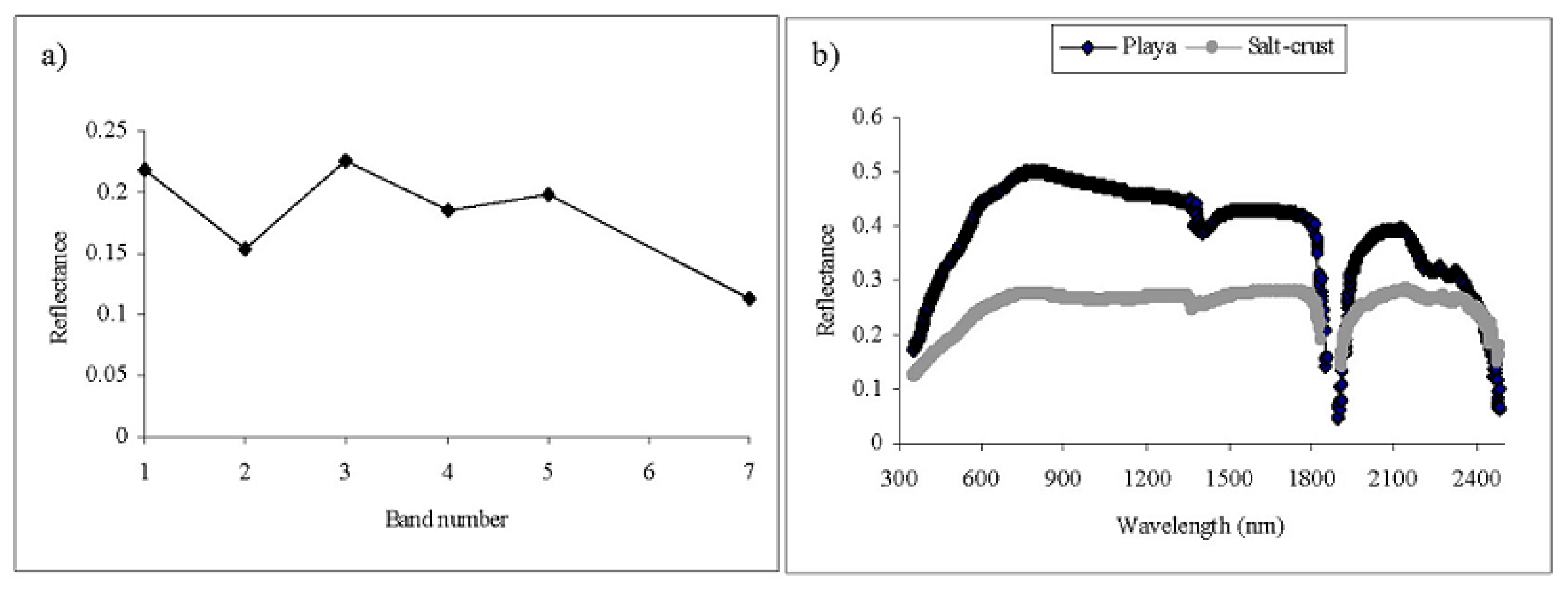
Salt-affected soils could easily be visually identified from the Landsat images using the false color composite (RGB 432) and brightness and wetness indices. The spectral reflectance curve (
Figure 2) shows that severely salt-affected soils have a high reflectance in the visual (bands 1, 2 and 3) and near infrared (band 4) parts of spectrum and relatively low reflectance in the mid-infrared parts of spectrum (bands 5 and 7). A significant correlation was found between the EC values and bands 1, 2, 3, and 4 of the Landsat images (
Table 4). Also, a significant correlation was found between the EC values and the brightness and wetness indices.
Figure 2.
Spectral reflectance of salt-affected soils collected by using (a) Landsat TM image and (b) Spectroradiometer. Spectral properties of salt-affected soils in the study area were measured in the field almost at the same acquisition time of Landsat TM images (August 17, 2005). The spectral reflectance was measured using the FieldspecfiPro, manufactured by Analytical Spectral Devices of Boulder Colorado. The instrument has a field of view of 25 mm. It covers the spectral range from 350 to 2,500 nm with an average bandwidth of 1 nm.
Landsat images were classified using the maximum likelihood supervised classifier in the ENVI program into 5 classes (1. Saline soil; 2. Agriculture land; 3. Inter-mountain basins big sage steppe; 4. Low sage brush steppe; and 5. Inter-mountain big sage brush shrubland) (
Figure 3). The output map was reclassified into two classes: saline (class 1) EC > 4 dSm
−1 and non-saline (classes 2, 3, 4, and 5) EC < 4 dSm
−1. Prediction accuracy of salt-affected soils was about 60% and non-saline soils was about 97%, with an overall accuracy was about 95%. Classified saline area represents 6.7% of the total area, whereas the non-saline area represents 93.3%.
3.3. Decision-Tree Analysis and Predicted Soil Salinity Map
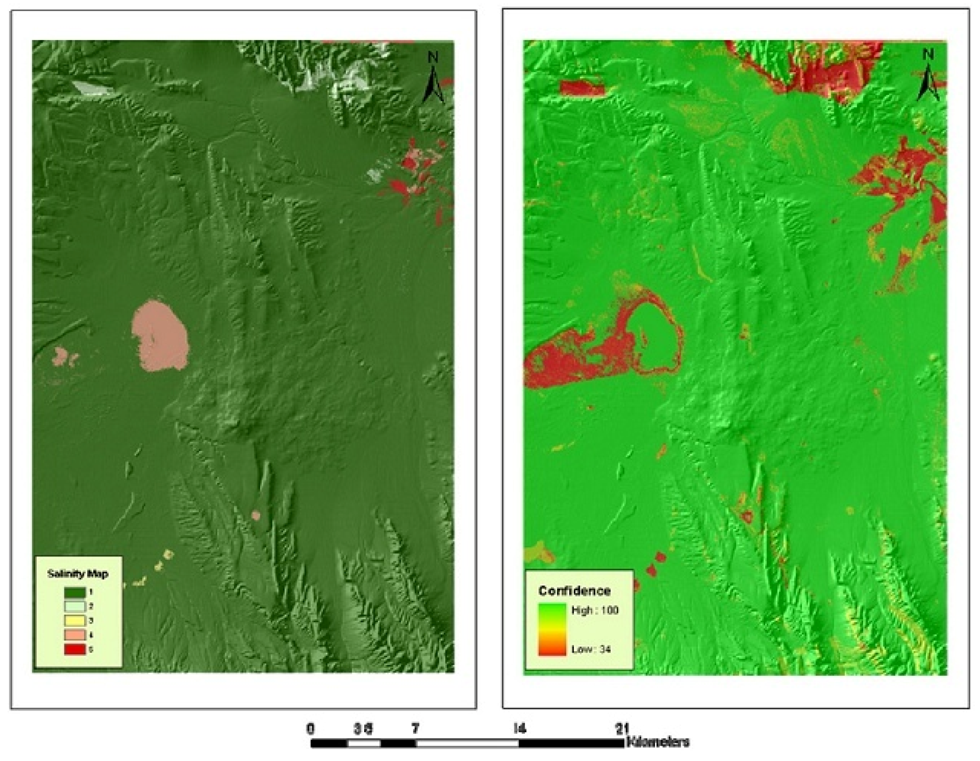
Decision-tree analysis yielded a predictive soil map with classes of salinity (
Figure 4). Prediction confidence in the classification accuracy of the decision tree is high (
Figure 4). The overall accuracy of the decision tree produced without boosting was 98.4% and Kappa coefficient was 0.90 (
Table 5). Producer’s accuracy varied from 77.7 to 99.2% with a mean value of 87.6%, whereas the user’s accuracy varied from 79.0 to 99.2% with a mean value of 85.8%. The prediction accuracy was enhanced by using 10 trials of boosting. The overall accuracy was 98.8% and Kappa coefficient was 0.92 (
Table 6). Producer’s accuracy varied from 78.8 to 99.2%, with a mean value of 91.4%, whereas the user’s accuracy varied from 71.0 to 99.6% with a mean value of 86.0%. The calculated area of saline soils represents 1.9% of the total area, whereas the non-saline area represents 97.4%.
Figure 3.
Supervised classification map of the Landsat TM image (1. Saline soil, 2. Agriculture land, 3. Inter-mountain basins big sage steppe, 4. Low sage brush steppe, and 5. Inter-mountain big sage brush shrubland).
Figure 3.
Supervised classification map of the Landsat TM image (1. Saline soil, 2. Agriculture land, 3. Inter-mountain basins big sage steppe, 4. Low sage brush steppe, and 5. Inter-mountain big sage brush shrubland).
Figure 4.
Predicted soil salinity map using decision tree analysis (left) and its prediction confidence (right). Class code 1 = codes 2-5 of
Figure 3; 2-5 = code 1 of
Figure 3. See also
Table 5.
Figure 4.
Predicted soil salinity map using decision tree analysis (left) and its prediction confidence (right). Class code 1 = codes 2-5 of
Figure 3; 2-5 = code 1 of
Figure 3. See also
Table 5.
Table 5.
Producer’s, user’s, overall accuracy and Kappa coefficient for predicted soil salinity classes developed without boosting.
Table 5.
Producer’s, user’s, overall accuracy and Kappa coefficient for predicted soil salinity classes developed without boosting.
Salinity
class |
Class1 |
Class2 |
Class3 |
Class4 |
Class5 | Total of rows | User’s accuracy |
|---|
| Class1 | 6961 | 15 | 5 | 12 | 23 | 7,016 | 99.22 |
| Class2 | 27 | 61 | | | | 88 | 69.32 |
| Class3 | 8 | | 30 | | | 38 | 78.95 |
| Class4 | 16 | | | 380 | 2 | 398 | 95.48 |
| Class5 | 7 | | | 7 | 87 | 101 | 86.14 |
| Total of columns | 7019 | 76 | 35 | 399 | 112 | 7,641 | |
| Producer’s accuracy | 99.17 | 80.26 | 85.71 | 95.24 | 77.68 | | 98.40 |
| Kappa | | | | | | | 0.90 |
Table 6.
Producer’s, user’s, overall accuracy and Kappa coefficient for predicted soil salinity classes developed with 10 trials of boosting.
Table 6.
Producer’s, user’s, overall accuracy and Kappa coefficient for predicted soil salinity classes developed with 10 trials of boosting.
Salinity
class | Class1 | Class2 | Class3 | Class4 | Class5 | Total of rows | User’s accuracy |
|---|
| Class1 | 6,987 | 17 | 3 | 4 | 5 | 7,016 | 99.59 |
| Class2 | 25 | 63 | | | | 88 | 71.59 |
| Class3 | 11 | | 27 | | | 38 | 71.05 |
| Class4 | 13 | | | 380 | 5 | 398 | 95.48 |
| Class5 | 7 | | | 1 | 93 | 101 | 92.08 |
| Total of columns | 7,043 | 80 | 30 | 385 | 103 | 7,641 | |
| Producer’s accuracy | 99.20 | 78.75 | 90.00 | 98.70 | 90.29 | | 98.81 |
| Kappa | | | | | | | 0.92 |
4. Discussion
Multi-class soil salinity maps are required for modern management of arid lands, and techniques such as that described here are needed to efficiently develop such inventories. Our results indicate that use of Landsat TM images of the study area well identifies bare areas that have a high reflectance due to their high salinity content and/or salt-efflorescence on the soil surface. This result agrees with that obtained by [
41] who reported that salt-affected soils with salt encrustation at the surface are, generally, smoother than non-saline surfaces and cause high reflectance in the visible and near-infrared bands. It was also noticed that the high spectral reflectance of some areas east and northeast of playas was due to millimeters-thin deposits of yellowish saline dust blown from the dry lake surfaces, resulting in misclassifying these locations as highly saline soils. Accordingly, classifying salt-affected soils based on spectral signatures could overestimate their areas.
Vegetation indices (NDVI, SAVI, and Greenness index) did not have a significant correlation with the EC values, which indicates that halophytes couldn’t be used in identifying salt-affected areas under vegetation cover. This could also be due to the coarse resolution of the Landsat image (30 m pixel size) and the smaller size of the salt-affected area. Landsat data could only distinguish between highly saline soils and normal or non-saline soils but salinity classes or degrees in between could not be discriminated. Similar results are noted by [
3] and [
12]. We also found that the wetness index has a significant correlation with the EC values which could be due to the tendency of salt-affected soils to retain high moisture content.
The soil salinity map developed by DTA successfully predicts five classes of salinity levels, a significant increase of the standard remote-sensing methods. This is likely due to the ability of DTA to integrate other environmental variables that have significant influence on the development of secondary salinization. Surficial geology and terrain attributes, notably elevation and slope, are critical variables in predicting soil salinity across such a broad area. We find that the difference between USGS 10 m DEM and IFSAR 5 m DEM to be significant in that the former partially or wholly misses key landforms with saline soils. Secondary salinization mostly occurs in low-land areas, where groundwater frequently rises up through the soil profile [
12,
38]. Therefore, it is important to identify these locations using the DEM. Soil salinity is not only influenced by the morphology of the soil profile but also by the soil physical, chemical and biological properties [
12,
42]. Bedrock geology and its chemical composition were integrated in the analysis and could result in enhancing the prediction accuracy. Soils in the study area are developed on Quaternary sediments and Tertiary volcanic flow rocks, mostly basalt and andesitic basalt, which are rich in feldspars and salt-bearing inclusions and vugs. Dominant vegetation is another variable that is directly influenced by higher soil salinity levels. This was also integrated in the analysis; however the vegetation map has a coarser scale that does not represent the vegetation types associated with soil salinity (halophytes), especially over smaller areas. This biological relationship to salinity is noted elsewhere across the study area, yet is not useful for large-scale distinctions of map classes.
5. Conclusions
Current remote-sensing methodology used in mapping soil salinity could be significantly improved if decision-tree analysis (DTA) is incorporated in such efforts. Remote-sensing data alone have been a nominally successful tool in mapping soil salinity over large areas, as it can only distinguish between two classes of saline soils: highly salt-affected soils, indicated by poor, sparse vegetation and high spectral reflectance, and non-saline soils, indicated by healthy vegetation. This is insufficient for modern soil salinity management with its five classes of salinity. Moreover, salt-affected areas may be overestimated when mapped using only spectral signatures.
The development of a soil salinity map additionally using DTA successfully distinguishes between the five classes of salinity used in the USA and elsewhere. DTA proved to be an efficient, useful approach for mapping soil salinity over large areas compared to traditional remote-sensing data. DTA incorporates several environmental variables that significantly influence the development of soil salinity and not only the spectral properties of the soil surface. The use of surficial geology, terrain and landform map layers, especially those developed using high-resolution IFSAR DEMs, significantly enhances delineations of map classes. Using this technique could significantly enhance the productivity and the accuracy of soil salinity mapping compared to conventional mapping methods especially in such remote inhospitable areas. Predictive maps of multi-class soil salinity should now be closer to obtain elsewhere around the world.
Acknowledgments
We gratefully acknowledge Mark Keller, Alina Rice, and Charlie Tackman of the Malheur County, Oregon, Soil and Ecological Survey for their support and accommodations. We thank Anne Nolin, for her assistance with the digital image analysis, Will Austin, for use of laboratory facilities for some of the salinity analyses, and Joan Sandeno, for editing an earlier version of this manuscript. Also, we thank our assistants Elizabeth Cervelli and Nathan Goodson for their field and laboratory work. This study was supported by funding from the Egyptian Cultural and Education Bureau, the Oregon Agricultural Experiment Station, and USDA-NRCS-National Geospatial Development Center Grant Award No. 68-3A75-4-101, mod 19. The authors are solely responsible for the content of this paper; any mention of proprietary names does not convey an endorsement by the governments of Egypt or the USA.
References and Notes
- Dwivedi, R.S.; Sreenivas, K. Image transforms as a tool for the study of soil salinity and alkalinity dynamics. Int. J. Rem. Sens. 1998, 19, 605–619. [Google Scholar] [CrossRef]
- Khan, N.M.; Rastoskuev, V.V.; Shalina, E.V.; Sato, Y. Mapping salt-affected soils using remote sensing indicators—a simple approach with the use of GIS-IDRSI. In Proceedings of the 22nd Asian Conference of Remote Sensing, Singapore, November; 2001. [Google Scholar]
- Mittermicht, G.I.; Zinck, J.A. Remote sensing of soil salinity: potentials and constraints. Remote Sens. Environ. 2003, 85, 1–20. [Google Scholar] [CrossRef]
- Sukchan, S.; Yamamoto, Y. Classification of salt affected areas using remote sensing and GIS. JIRCAS Working Report 2002, 30, 15–19. [Google Scholar]
- Burough, P.A. Principles of Geographical Information Systems for Land Resources Assessment; Oxford University Press: New York, NY, USA, 1986; p. 193. [Google Scholar]
- Hansen, M.; Dubayah, R.; Defries, R. Decision trees: an alternative to traditional land cover classifiers. Int. J. Rem. Sens. 1996, 17, 1075–1081. [Google Scholar] [CrossRef]
- McBratney, A.B.; Mendonca Santos, M.L.; Minasny, B. On digital soil mapping. Geoderma 2003, 117, 3–52. [Google Scholar] [CrossRef]
- Qi, F.; Zhu, A.X. Knowledge discovery from soil maps using inductive learning. Int. J. Geog. Inf. Sci. 2003, 17, 771–795. [Google Scholar] [CrossRef]
- Scull, P.; Franklin, J.; Chadwick, O.A. The application of decision tree analysis to soil type prediction in a desert landscape. Ecol. Model. 2005, 181, 1–15. [Google Scholar] [CrossRef]
- Olea, R.A. Geostatistics for Engineers and Earth Scientists; Kluwer Academic Publishers: Boston, MA, USA, 1999. [Google Scholar]
- Pozdyakova, L.; Zhang, R. Geostatistical analyses of soil salinity in a large field. Prec. Ag. 1999, 1, 153–65. [Google Scholar] [CrossRef]
- Sethi, M.; Dasog, G.S.; Lieshout, A.V.; Salimath, S.B. Salinity appraisal using IRS images in Shorapur Taluka, Upper Krishna Irrigation Project, Phase I, Gulbarga District, Karnataka. India. Int. J. Remote Sens. 2006, 27, 2917–2926. [Google Scholar] [CrossRef]
- Huang, C.; Davis, L.S.; Townshend, J.R.G. An assessment of support vector machines for land cover classification. Int. J. Rem. Sens. 2002, 23, 725–749. [Google Scholar] [CrossRef]
- Venables, W.N.; Ripley, B.D. Modern Applied Statistics with S-PLUS; Springer-Verlag: New York, NY, USA, 1994. [Google Scholar]
- Csillag, F.; Pasztor, L.; Biehl, L.L. Spectral band selection for the characterization of salinity status of soils. Remote Sens. Environ. 1993, 43, 231–242. [Google Scholar] [CrossRef]
- Joshi, M.D.; Sahai, B. Mapping salt-affected land in Saurashtra coast using Landsat satellite data. Int. J. Rem. Sens. 1993, 14, 1919–1029. [Google Scholar] [CrossRef]
- Manchanda, M.L. Use of remote sensing techniques in the study of distribution of salt-affected soils in north-west India. Indian Soc. Soil Sci. 1984, 32, 701–706. [Google Scholar]
- Sharma, R.C.; Bhargawa, G.P. Landsat imagery for mapping saline soils and wetlands in north-west India. Int. J. Remote Sens. 1988, 9, 69–84. [Google Scholar] [CrossRef]
- Singh, A.N.; Kristof, S.J.; Baumgardner, M.F. Delineating Salt-Affected Soils in the Ganges Plain, India by Digital Analysis of Landsat Data; LARS Techical Report 111477; The Laboratory of Applications of Remote Sensing: Purdue University, West Lafayette, IN, USA, 1977. [Google Scholar]
- Spies, B.; Woodgate, P. Salinity Mapping Methods in the Australian Context; Department of the Environment and Heritage, and Agriculture, Fisheries and Forestry: Canberra, Australia, 2005. [Google Scholar]
- Schoeneberger, P.J.; Wysocki, D.A.; Benham, E.C.; Broderson, W.D. Field Book for Describing and Sampling Soils, Version 2.0; Natural Resources Conservation Service, National Soil Survey Center: Lincoln, NE, USA, 2002. [Google Scholar]
- Soil Survey of Elko County, Northeastern Part; Natural Resources Conservation Service, US Department of Agriculture: Washington, DC, USA, 1999.
- Soil Taxonomy, 9th ed.Natural Resources Conservation Service, US Department of Agriculture: Washington, DC, USA, 2003.
- Clarke, S.E.; Bryce, S.A. Hierarchical Subdivisions of the Columbia Plateau and Blue Mountains Ecoregions, Oregon and Washington; US Department of Agriculture-Forest Service General Technical Report PNW-GTR-395; Portland, OR, USA, 1997; p. 114. [Google Scholar]
- Kagan, J.; Caicco, S. Manual of Oregon Actual Vegetation; Idaho Cooperative Fish and Wildlife Research Unit, University of Idaho: ID, USA, 1992. [Google Scholar]
- LANDSAT TM-Path: 42 Row: 30 for Scene: 5042030000519810 and Path: 42 Row: 31 for Scene: 5042031000519810; US Geological Survey Center for Earth Resources Observation and Science (EROS): Sioux Falls, SD, USA, 2005.
- Rouse, J.W.; Haas, R.H.; Schell, J.A.; Deering, D.W. Monitoring vegetation systems in the Great Plains with ERTS. In Proceedings of Third ERTS Symposium, Washington, DC, WA, USA; 1973; pp. 309–317. [Google Scholar]
- Huete, A. A soil-adjusted vegetation index (SAVI). Remote Sens. Environ. 1988, 25, 295–309. [Google Scholar] [CrossRef]
- Kauth, R.J.; Thomas, G.S. The tasseled cap: a graphic description of the spectral-temporal development of agricultural crops as seen by LANDSAT. In Proceedings of the Symposium on Machine Processing of Remotely Sensed Data; Purdue University of West Lafayette: West Lafayette, IN, USA, 1976; pp. 4B-41–4B-51. [Google Scholar]
- Landfire Existing Vegetation Cover; USDA Forest Service: Missoula, MT, USA, 2006.
- Oregon Annual Precipitation; National Cartography and Geospatial Center: USDA-NRCS, Fort Worth, TX, USA, 1999.
- Miller, R.J.; Raines, G.L.; Connors, K.A. Spatial Digital Database for the Geologic Map of Oregon; USGS Open File Report 03-67; Menlo Park, CA, USA, 2003. [Google Scholar]
- De Gruitjer, J.J. Sampling for Spatial Inventory and Monitoring of Natural Resources; Technical report, Alterrrarapport 070; Green World Research: Alterra, Wageningen, The Netherlands, 2000. [Google Scholar]
- Richards, L.A. Diagnosis and improvement of saline and alkali soils. In Agriculture Handbook No. 60; US Department of Agriculture: Washington, DC, USA, 1954. [Google Scholar]
- Rowan, L.C.; Goetz, A.F.H.; Ashley, R.P. Discrimination of hydrothermally altered and unaltered rocks in the visible and the near infrared multispectral images. Geophysics 1977, 42, 522–535. [Google Scholar] [CrossRef]
- Riaza, A.; Mediavilla, R.; Santistieban, J.I. Mapping geological stages of climate-dependent iron and clay weathering alteration on lithologically uniform sedimentary units using Thematic Mapper imagery (Tertiary Duero Basin, Spain). Int. J. Rem. Sens. 2000, 21, 937–950. [Google Scholar] [CrossRef]
- Quinlan, J.R. C4.5: Programs for Machine Learning; Morgan Kaufmann Publishers Inc.: San Francisco, CA, USA, 1993. [Google Scholar]
- Eklund, D.P.W.; Kirkby, S.D.; Salim, A. Data mining and soil salinity analysis. Int. J. Geog. Inf. Sci. 1998, 12, 247–268. [Google Scholar] [CrossRef]
- Earth Satellite Corporation. CART Software User’s Guide; Earth Satellite Corporation: Washington, DC, USA, 2003. [Google Scholar]
- Freund, Y.; Schapire, R. Experiments with a new boosting algorithm. In Proceedings of the Thirteenth International Conference on Machine Learning, San Mateo, CA, USA; 1996. [Google Scholar]
- Everitt, J.; Escobar, D.; Gerbermann, A.L.; Alaniz, M. Detecting saline soils with video imagery. Photogramm. Eng. Rem. Sens. 1988, 54, 1283–1287. [Google Scholar]
- Szabolcs, I. The global problems of salt-affected soils. Acta Agron. Hung. 1987, 36, 159–172. [Google Scholar]
© 2010 by the authors; licensee Molecular Diversity Preservation International, Basel, Switzerland. This article is an open-access article distributed under the terms and conditions of the Creative Commons Attribution license (http://creativecommons.org/licenses/by/3.0/).


