Interferometric vs Spectral IASI Radiances: Effective Data-Reduction Approaches for the Satellite Sounding of Atmospheric Thermodynamical Parameters

Abstract

Two data-reduction approaches for the Infrared Atmospheric Sounder Interferometer satellite instrument are discussed and compared. The approaches are intended for the purpose of devising and implementing fast near real time retrievals of atmospheric thermodynamical parameters. One approach is based on the usual selection of sparse channels or portions of the spectrum. This approach may preserve the spectral resolution, but at the expense of the spectral coverage. The second approach considers a suitable truncation of the interferogram (the Fourier transform of the spectrum) at points below the nominal maximum optical path difference. This second approach is consistent with the Shannon-Whittaker sampling theorem, preserves the full spectral coverage, but at the expense of the spectral resolution. While the first data-reduction acts within the spectral domain, the second can be performed within the interferogram domain and without any specific need to go back to the spectral domain for the purpose of retrieval. To assess the impact of these two different data-reduction strategies on retrieval of atmospheric parameters, we have used a statistical retrieval algorithm for skin temperature, temperature, water vapour and ozone profiles. The use of this retrieval algorithm is mostly intended for illustrative purposes and the user could choose a different inverse strategy. In fact, the interferogram-based data-reduction strategy is generic and independent of any inverse algorithm. It will be also shown that this strategy yields subset of interferometric radiances, which are less sensitive to potential interfering effects such as those possibly introduced by the day-night cycle (e.g., the solar component, and spectroscopic effect induced by sun energy) and unknown trace gases variability.

1. Introduction

The Infrared Atmospheric Sounding Interferometer (IASI) is providing data of unprecedented spectral quality and accuracy (see e.g., [1]). The assimilation of IASI radiances has produced a significant positive impact on forecast quality (e.g., [2]) and on the exploitation of trace gases information for atmospheric chemistry.

IASI has been developed in France by the Centre National d’Etudes Spatiales (CNES) and is flying on board the Metop-A (Meteorological Operational Satellite) platform, the first of three satellites of the European Organization for the Exploitation of Meteorological Satellite (EUMETSAT) European Polar System (EPS).

IASI has been primarily put in orbit to work for a meteorological mission, hence its main objective is to provide suitable information on temperature and water vapour profiles. The instrument has a spectral coverage extending from 645 to 2,760 cm${}^{-1}$, which with a sampling interval $\Delta \sigma =0.25$ cm${}^{-1}$ gives 8,461 data points or channels for each single spectrum. Data samples are taken at intervals of 25 km along and across track, each sample having a minimum diameter of about 12 km. With a swath width on Earth’s surface of about 2,000 kilometres, global coverage is achieved in 12 hours, during which the instrument records about 650,000 spectra.

This large amount of data is still now hampering the full exploitation of IASI data at Numerical Weather Prediction (NWP) centers, and in all those situations in which we have the constraint of processing the data in near real time. As an example, to reduce the significant computational burden, of the $N_{IASI}=8461$ channels received at the European Centre for Medium Range Weather Forecasts (ECMWF) only $N=366$ are routinely monitored [2] and even less ($N=168$) are actively assimilated.

However, whatever the methodology or selection rules we apply, any channels reduction directly performed in the spectral domain, which yields a sparse sub-set of N radiances with $N<N_{IASI}$, violates the Shannon-Whittaker sampling theorem (e.g., [3]) and, therefore, occurs at expense of the full IASI spectral coverage, and irreversibly destroys that information which is contained in the portion of the spectrum or set of channels we do not use.

Conversely, if we first Fourier transform the full IASI spectrum, in order to get the interferogram, and second we just truncate the interferogram and retain only the first N out of $N_{IASI}$ samples, we perform a channel interpolation, which is consistent with the Shannon-Whittaker sampling theorem and, therefore, leaves unchanged the full IASI spectral coverage.

Having in mind mainly the retrieval of thermodynamical parameters (temperature and water vapour), the main objective of this study is to demonstrate, with IASI retrieval exercises, the use of the interferogram-based data reduction approach and compare it to channels selection rules (e.g., [4]), which work directly in the spectral domain. As said, the intercomparison will be performed by performing a series of IASI retrieval exercises for temperature, water vapour and ozone, based on subsets of IASI channels obtained with both the interferogram-based data reduction truncation approach and the selection of sparse spectral channels, respectively.

Data-reduction performed directly in the wave number domain by picking up suitable channels saves the spectral quality of the data (i.e., spectral resolution), but, conversely, it applies no filter to the noise, and destroys the initial full spectral coverage.

On the other hand, truncation in the interferogram domain saves the full spectral coverage, reduces the noise because we reduce its bandwidth, but degrades the spectral quality.

According to [5] spectral resolution is important to have peaked weighting functions for temperature. However, other authors [6,7] who addressed the problem of vertical spatial resolution in the context of the interferogram domain found out that the sharpness of weighting functions can even increase considering interferogram rather than spectral radiances.

It is fair to say that there is an alternative to the Fourier transform of the spectrum in order to use information from all IASI channels. This relies on a different kind of linear transform, which is the Empirical Orthogonal Functions (EOF) or Principal Component Analysis (PCA) transform (e.g., [8], see also [9] for a review on the application of EOF to the field of satellite meteorology). Then, instead of truncating the interferogram radiances, we truncate the PC scores.

The advantage of the EOF transform is that, by truncation, not only we save the full spectral coverage as in the case of the Fourier transform, but we retain most of the spectral quality, because of the effectiveness of the EOF transform to represent complex but highly redundant signals (as it is the case of atmospheric spectra) with few PC scores. It might seem that the EOF transform makes the kind of magic we need. However, in case we EOF transform the full spectrum, the results is to retain all those factors, which may potentially interfere with the temperature and water vapour retrieval process and add biases to the final products.

Thus, while the EOF approach remains appealing for data compression, it does not solve the problem of alleviating the effect of interfering factors when we use the data for retrieval purposes, unless we remove from the spectral coverage those interfering portions of the spectrum. However, once again this approach would sacrifice the full IASI spectral range and make one work with a partial coverage.

The potential interfering factors include minor species (e.g., methane and carbon monoxide), which are normally not retrieved in the context of meteorological applications, and therefore could add more uncertainty to the final products of temperature and water vapour. In addition, the IASI spectrum extends to the side of short wave numbers 2,100 to 2,760 cm${}^{-1}$. At these wave numbers the energy measured from IASI contains a mixture of earth and solar spectra, which may introduce (for daytime spectra) further computational burden and uncertainty in the final products. Moreover, during daytime the core of the CO${}_2$ ${\nu }_3$-band is influenced by non Local Thermodynamic Equilibrium (non LTE), which further complicate the use of the short wave side of the spectrum.

To this respect, the appealing characteristic of the Fourier transform is that it also carries out the task of transforming very localized and narrow-band spectral features in new ones, which are broadened, distributed and diluted over the entire variability range of the transformed data space, so that they may become negligible with respect to the strong signal introduced by temperature and water vapour. Thus, even if we want to maintain the machinery of EOF transform within our retrieval scheme, it would be desirable to first project the data space in a new (orthogonal) one having the characteristics outlined above.

It is also important to stress, at this point, that the above projection is what a Fourier transform spectrometer (FTS), such as IASI, automatically provides when it measures the interferogram, which, in fact, is the Fourier transform of the spectrum.

Since the spectrum is the linear Fourier transform of the interferogram, and conversely, in general they bring the same information. However, the situation we discuss here is not perfectly symmetric, since for the spectral domain we use only a partial coverage because of the problem of avoiding interfering effects and the prohibitive computational effort for real time applications. For the case of the interferogram we use a truncated version of the interferogram, which has the effect of reducing the number of data points, but still preserving the full spectral coverage. The equivalence between the two spaces is also broken because of noise. In the spectral domain the noise can be correlated because of mathematical apodization, such as that applied to IASI. Conversely even with mathematical apodization in the inteferogram domain the noise is fairly constant in strength (variance) and is uncorrelated. Finally the signal-to-noise ratio is higher in the interferogram space than in the spectral domain.

As said before, the use of the interferogram instead of the spectrum for the retrieval of atmospheric parameters is not completely new. It was first suggested and discussed in [6,7] for the case of temperature. In [6,7] the authors also argued that the interferogram domain could improve the vertical spatial resolution of the retrievals because of weighting functions, which are sharper of those available in the spectral domain. However, until now the method has non been demonstrated on the basis of real observations.

As already outlined before, the main objective of this paper is to illustrate, demonstrate and exemplify the potential advantages of the interferogram-based data reduction and retrieval over those provided by the spectrum, through the exploitation of IASI data.

Towards this objective, we have used a retrieval methodology, which is based on a linear regression algorithm, in which the data space (spectral radiance domain or interferometric radiance domain) is further transformed via EOF in order to reduce the dimensionality of the inverse problem. The EOF regression approach has been used by many authors, among which we refer to [9,10,11,12,13]).

The paper is organized as follows. In Section 2 we describe the basic aspects of our interferogram-based data-reduction approach, along with information relevant to forward and inverse calculations. In Section 3 we describe two different subsets of IASI channels for the purpose of near real time dissemination and retrieval processing of IASI data. A series of retrieval exercises exploiting the reduced data sets of IASI channels will be presented and discussed in Section 4. Conclusions are drawn in Section 5.

2. Methodological Background: Data Reduction Principles, Forward/Inverse Methodology

2.1. The Fourier Pair: Spectrum, $R\left(\sigma \right)$, Interferogram, $I\left(x\right)$

The emission spectrum $R\left(\sigma \right)$, σ being the wave number, of a given source is physically defined in the interval $[0,\infty ]$. However, according to the Shannon Whittaker sampling theorem [3], only bandlimited functions can be effectively sampled without loss of information. In practice, the band-limited property is achieved by suitable optical filtering, so that the spectrum $R\left(\sigma \right)$ may be mathematically represented by the band-limited function,

$$R\left(\sigma \right)=\left\{\begin{array}{c}\text{arbitrary for} {\sigma }_1\le \sigma \le {\sigma }_2\\ 0\mathrm{otherwise}\end{array}\right.$$

(1)

where ${\sigma }_2-{\sigma }_1$ is the bandwidth of the spectrum signal.

To cope with the symmetry of the Fourier transform and for a correct application of the convolution theorem, formal mathematical calculations employ the even function $R_t\left(\sigma \right)$, defined in the interval $[-\infty ,+\infty ]$: $R_t(-\sigma )=R_t\left(\sigma \right)$, $R_t\left(\sigma \right)=R\left(\sigma \right)/2$. Note that this definition leaves the total energy unchanged, that is,

$${\int }_{-\infty }^{+\infty }{R}_t\left(\sigma \right)d\sigma ={\int }_0^{+\infty }R\left(\sigma \right)d\sigma$$

(2)

The function $R\left(\sigma \right)$ is often referred to as the one-sided spectrum, whereas $R_t\left(\sigma \right)$ is the two-sided spectrum. The interferogram $I\left(x\right)$, which is the function actually measured, e.g., by Fourier Transform Spectrometers, is then the Fourier transform of $R_t\left(\sigma \right)$.

$$I\left(x\right)={\int }_{-\infty }^{+\infty }{R}_t\left(\sigma \right)exp(-2\pi i\sigma x)d\sigma$$

(3)

with i the imaginary unit. Note that $I\left(x\right)$ is itself an even function, and x is a spatial coordinate, physically related to the optical path difference of the two light beams that travel in the interferometer. If we know, $I\left(x\right)$, then $R_t\left(\sigma \right)$ can be recovered by considering the inverse Fourier transform,

$$R_t\left(\sigma \right)={\int }_{-\infty }^{+\infty }I\left(x\right)exp\left(2\pi i\sigma x\right)dx$$

(4)

It should be stressed that the a Fourier pair, ($R\left(\sigma \right),I\left(x\right)$) can be defined independently of he instrument we use to acquire either of $R\left(\sigma \right)$ and $I\left(x\right)$. Although, for an interferometer spectrometer, $I\left(x\right)$ has a physical meaning, here we are interested in the mathematical properties of the transform itself. Thus, the fact that IASI spectra are, e.g, apodized is of no important concern in the analysis. We just consider the Fourier transform of these apodized spectra.

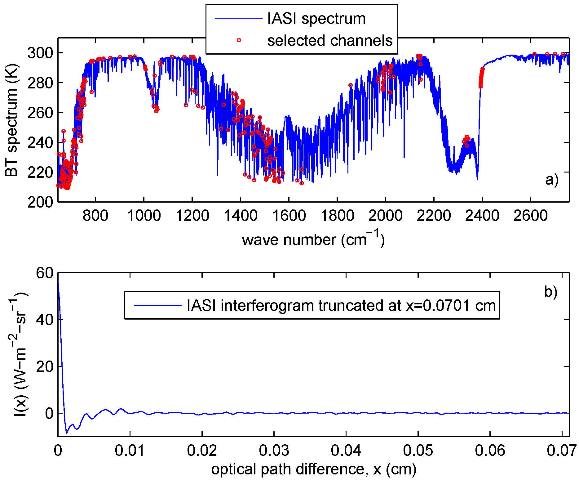
Coming now to the particular case of IASI, Figure 1 exemplifies a couple $\left(R\left(\sigma \right),I\left(x\right)\right)$ for this instrument. According to the Shannon-Whittaker sampling theorem [3], the Fourier transform provides the right mathematics to sample the band-limited function, $R\left(\sigma \right)$ to, e.g., a sampling rate different from the original one. This involves the well-known Nyquist rule about the two sampling rates, $\Delta \sigma$ and $\Delta x$ in the spectral and interferogram domain, respectively,

$$\Delta \sigma =\frac{1}{2x_{max}},\Delta x=\frac{1}{2({\sigma }_2-{\sigma }_1)}$$

(5)

where $x_{max}$ is the maximum optical depth and, as before, ${\sigma }_2-{\sigma }_1$ is the spectral bandwidth. For IASI we have ${\sigma }_1=645$ cm${}^{-1}$, ${\sigma }_2=2760$ cm${}^{-1}$ and $x_{max}=2$ cm.

In case we want to re-sample the IASI spectrum at a new rate, say $\Delta {\sigma }^{*}$, the operations involved consist in

• Fourier transform the spectrum to the interferogram domain
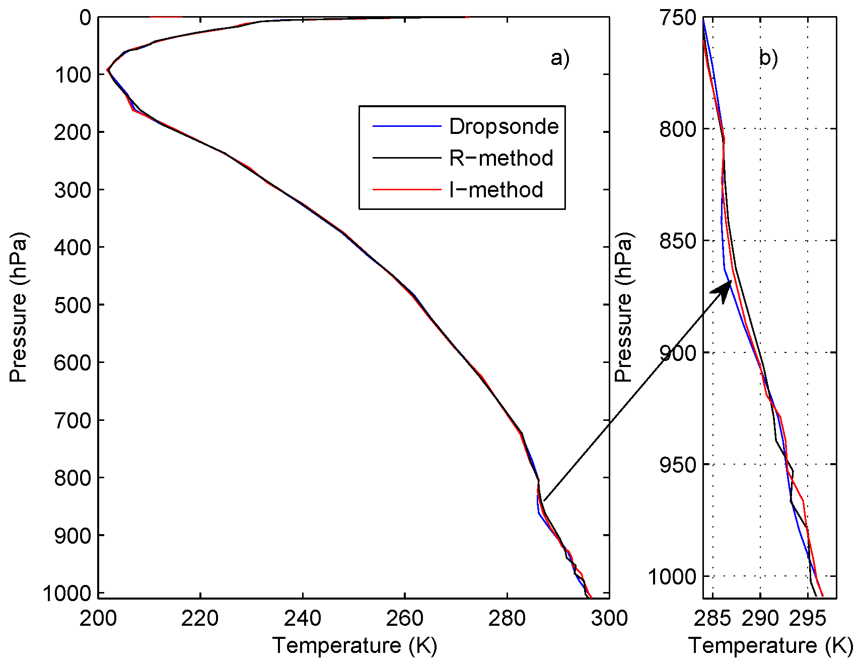
  Figure 1. Example of IASI observed spectrum, $R\left(\sigma \right)$, shown in panel (a), and its mathematical Fourier transform, $I\left(x\right)$, shown in panel (b). The behaviour of $I\left(x\right)$ close to $x=0$ is shown in the inset. The interferogram interval [0,0.8] cm has been drawn in red in panel (b).

  Figure 1. Example of IASI observed spectrum, $R\left(\sigma \right)$, shown in panel (a), and its mathematical Fourier transform, $I\left(x\right)$, shown in panel (b). The behaviour of $I\left(x\right)$ close to $x=0$ is shown in the inset. The interferogram interval [0,0.8] cm has been drawn in red in panel (b).
• cut the interferogram at a new $x_{max}^{*}=1/(2\Delta {\sigma }^{*})$
• transform back the truncated interferogram to the spectral domain.

An alternative processing approach, which yields the same result, could be to use a suitable cardinal sine (or sinc function) interpolation in the spectral domain. This would avoid the passage through the interferogram domain. However, we prefer to use the method outlined above, since we want also to show that the processing chain for the retrieval of atmospheric parameters can be validly performed in the interferogram domain.

However, either we transform to the interferogram domain or we simply apply a sinc interpolation in the spectral domain, the operation leaves unchanged the spectral coverage, while it changes the spectral sampling from $\Delta \sigma$ to $\Delta {\sigma }^{*}$.

As anticipated in Figure 1, if we truncate the interferogram at $x_{max}=0.8$ cm${}^{-1}$ and take the inverse Fourier transform back to the spectral domain, we have the spectrum with the new sampling $\Delta \sigma =0.625$ cm${}^{-1}$, instead of the original one of $\Delta \sigma =0.25$ cm${}^{-1}$. Furthermore, the original 8,461 spectral data points, would be scaled down by a factor which is equal to the ratio of the two samplings, so that we are left with 3,385 data points.

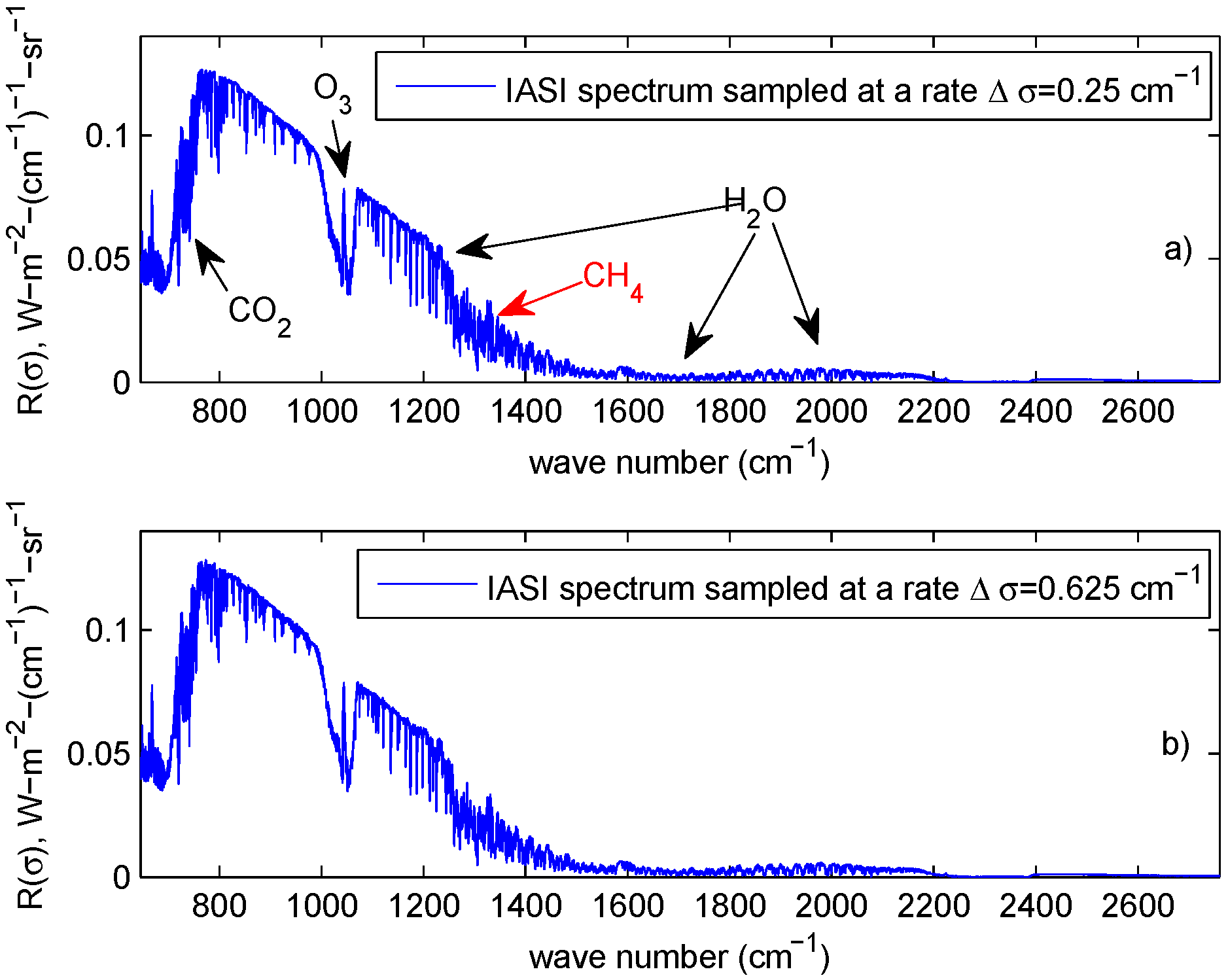
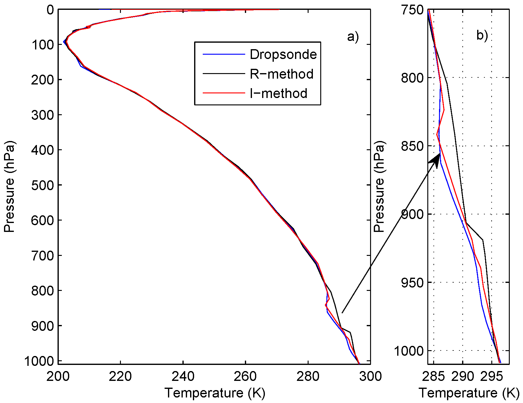
An example of these two spectra is shown in Figure 2. Although illustrative, Figure 2 shows that the re-sampling from $\Delta \sigma =0.25$ cm${}^{-1}$ to $\Delta \sigma =0.625$ cm${}^{-1}$ leaves almost unchanged the spectral quality of the spectrum in the three bands, 645 to 800 cm${}^{-1}$, 900 to 1,000 cm${}^{-1}$, 1,200 to 2,000 cm${}^{-1}$, which are important for the sounding of temperature, ozone and water vapour, respectively.

Figure 2. Example of IASI spectrum, $R\left(\sigma \right)$, sampled at the nominal rate $\Delta \sigma =0.25$ cm${}^{-1}$, shown in panel (a), and $\Delta \sigma =0.625$ cm${}^{-1}$, shown in panel (b). The plot in panel (a) also shows the main absorption features due to CO${}_2$, CH${}_4$, H${}_2$O and O${}_3$.

Figure 2. Example of IASI spectrum, $R\left(\sigma \right)$, sampled at the nominal rate $\Delta \sigma =0.25$ cm${}^{-1}$, shown in panel (a), and $\Delta \sigma =0.625$ cm${}^{-1}$, shown in panel (b). The plot in panel (a) also shows the main absorption features due to CO${}_2$, CH${}_4$, H${}_2$O and O${}_3$.

Temperature sounding is mainly performed by exploiting the CO${}_2$ longwave band at 15 μm. To improve temperature retrieval, it is important that this band is sampled at a rate better than $\Delta \sigma$ = 0.8 cm${}^{-1}$. Doing so, we can see in the ${\nu }_2$ absorption band of CO${}_2$ a characteristic periodic pattern, in which relatively transparent channels alternate with more opaque channels. This is a result of the fact that the ${\nu }_2$ fundamental band of CO${}_2$ is coupled with rotational transitions, which yield that periodic structure. This structure allows us to sense also the wings of the lines, which, according to [5], have the sharpest weighting functions for temperature.

The regular spacing of the CO${}_2$ lines introduce a very strong signature in the interferogram, as well. The signature can be seen in Figure 1 around $x=0.625$ cm and provides a very nice example of the fact, we have mentioned so far, that broad features in one domain, such as periodic behaviour, are transformed in narrow-band, sharp features in the other. Since the line spacing in the ${\nu }_2$ band of CO${}_2$ has a regular size of about 1.6 cm${}^{-1}$, we have to expect a sharp signature at $x=n/1.6$ cm, with $n=1,2,3,...$ an integer number. For $n=1$, we have $x=0.625$ cm. This signature is clearly identified in the interferogram of Figure 1. On passing, it should be noted that the signature for $n=2$, that is at 1.25 cm is barely visible because of IASI Gaussian apodization.

The vibration-rotational bands of H${}_2$O at 6.7 μm and O${}_3$ at 9.6 μm do not yield a regular spacing of the rotational lines, therefore, unlike CO${}_2$, for the case of ozone and water vapour there is not a precise prescription for the sampling rate. Furthermore, neither at 0.25 cm${}^{-1}$ nor at 0.625 cm${}^{-1}$ we can insulate single lines of ozone or water vapour. In other words, the prescription for a sampling better than 0.8 cm${}^{-1}$ is driven by temperature retrieval.

Having in mind the retrieval for temperature, water vapour and ozone, the above discussion lead us to conclude that there is no need to use the 0.25 cm${}^{-1}$ sampled IASI spectrum, since the spectrum sampled at 0.625 cm${}^{-1}$ brings the same spectral information for temperature, water vapour and ozone.

However, it is important to stress that for chemistry studies the sampling at 0.625 cm${}^{-1}$ could be not enough.

Another important aspect of the interferogram steams directly from its definition. According to Equation 3 the interferogram at $x=0$ measures the total energy in the spectrum. Therefore, spectral characteristics, which are locally intense in the spectrum but express few energy, add a very little contribution to the interferogram. It is evident from Figure 1 or Figure 2, which most of the energy in the IASI spectrum is explained from the range 645 to 2,000 cm${}^{-1}$. 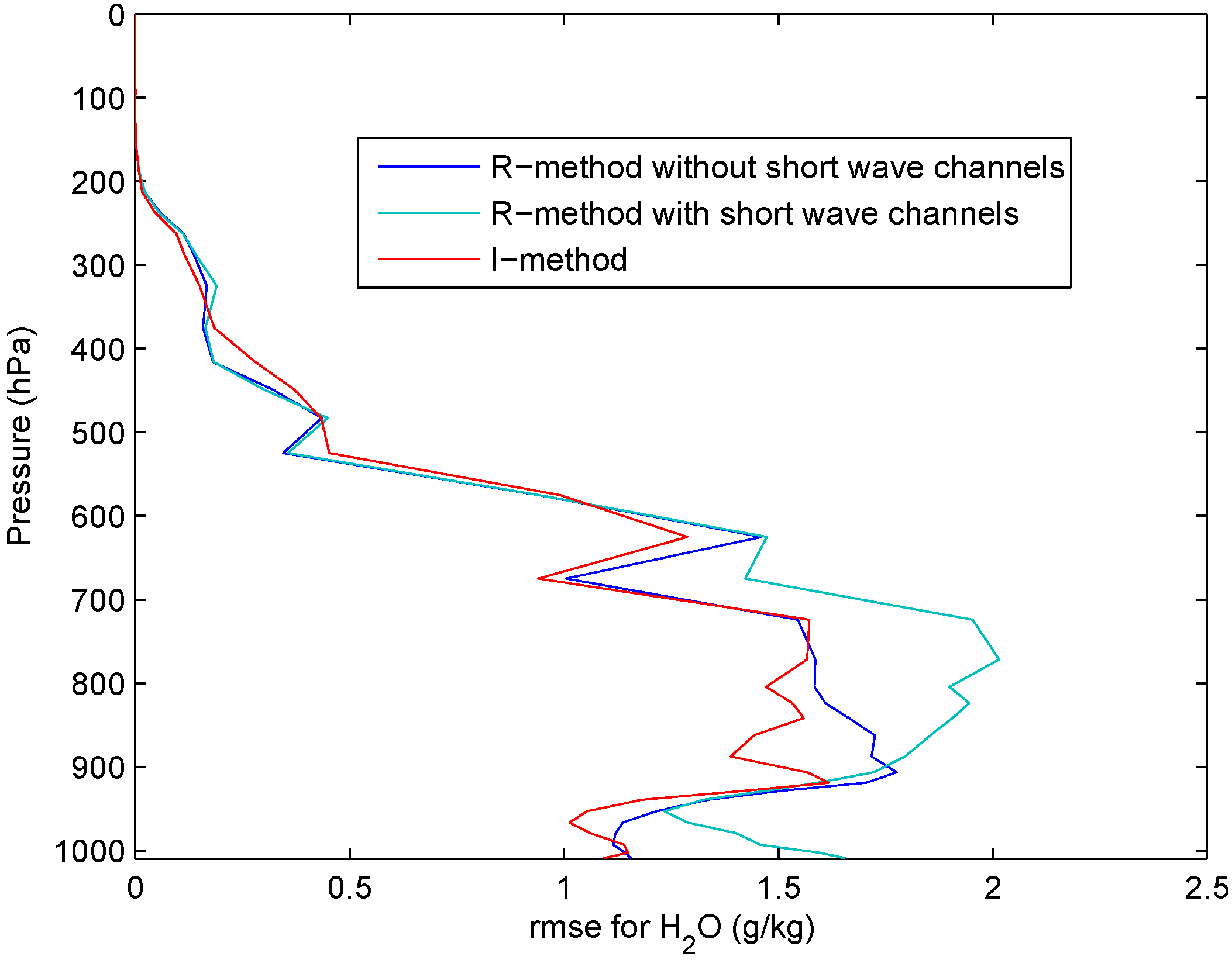Thus, variability which occurs in IASI band 3 (2,000 to 2,760 cm${}^{-1}$), adds second order effects to the interferogram. This is the case, e.g., of the solar energy during the day, which has its larger effect in the short-wave side of the spectrum (IASI band 3). However, while the solar energy greatly affects IASI band 3, its contribution to the total energy is not larger than 0.5%. In the same way, also spectroscopic effects, such as non LTE that are mostly concentrated in IASI band 3, become negligible once considered in the interferogram domain.

In general, localized absorption features, which need a very high spectral resolution to be revealed in the spectrum, add only very few energy to the spectrum itself. In the conjugate Fourier domain, they contribute to the interferogram with a very long wave-train, which need to be recorded on a very long distance (optical path difference) in order to be recovered. Thus, truncating the spectrum is also a way to loose information on the trace gases, and can act as a sort of filtering for interfering factors.

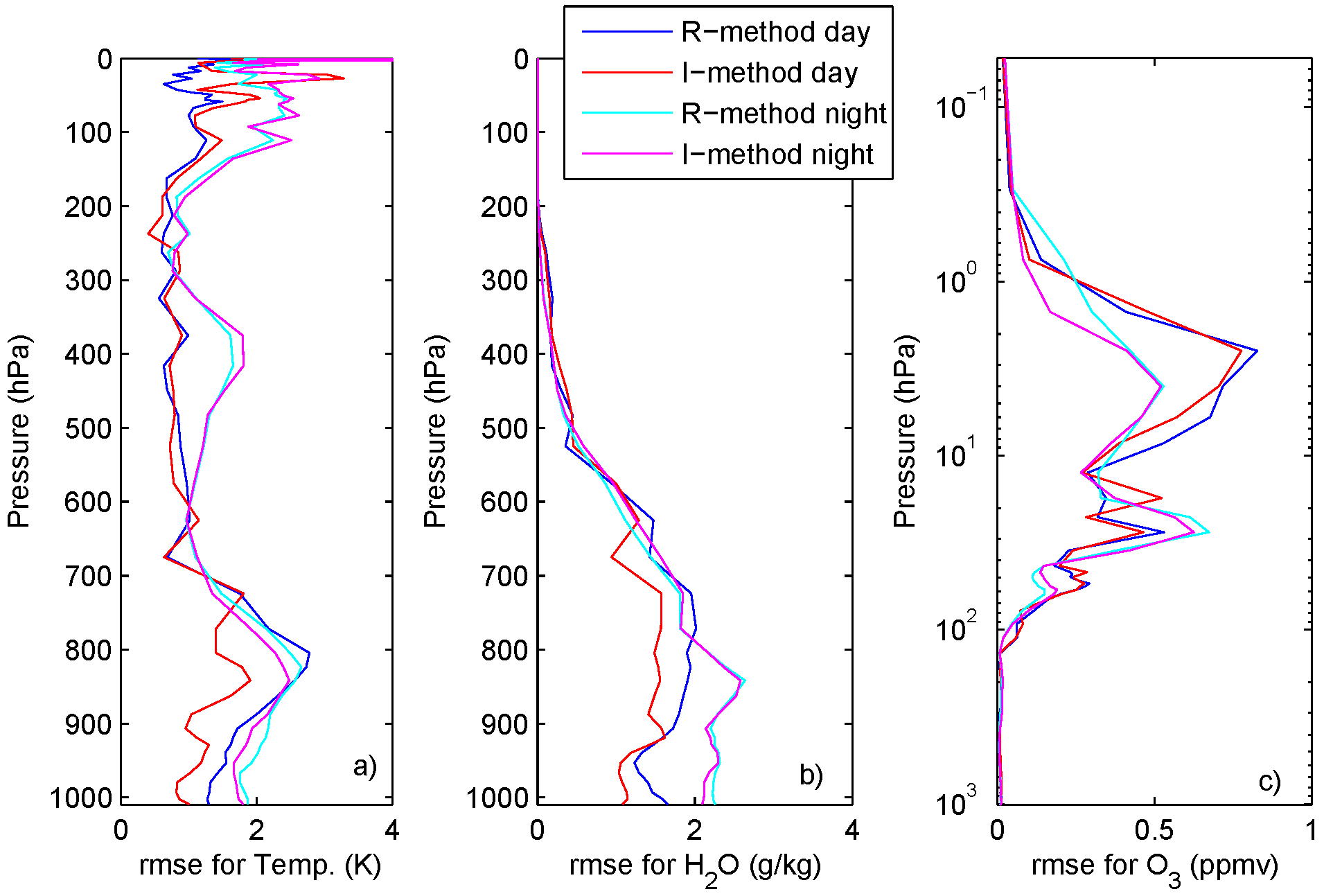
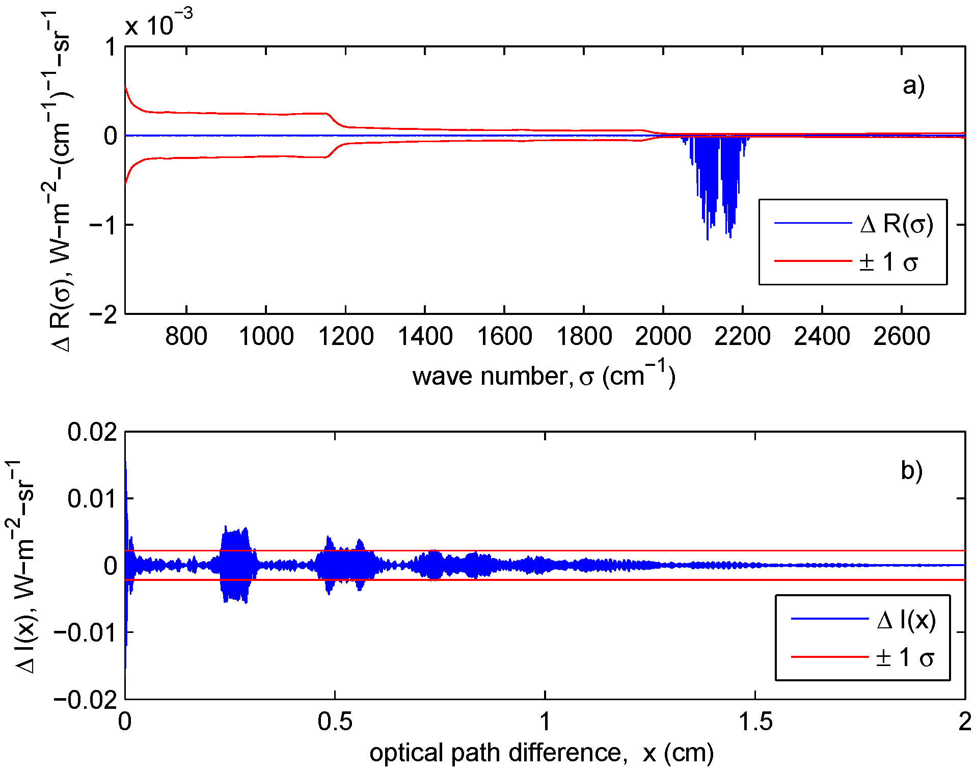
This effect is exemplified in Figure 3 for the CO absorption band in the IASI band 3. The figure shows the difference, $\Delta R\left(\sigma \right)=R\left(\sigma \right)-R_0\left(\sigma \right)$ between a synthetic IASI spectrum, $R\left(\sigma \right)$ with CO set to its climatological load, and a reference, $R_0\left(\sigma \right)$ without any load of CO. The corresponding $\Delta I\left(x\right)$ is shown in the same figure.

It is seen that in the spectral domain, the CO absorption produces a narrow-band signal, which is very sharp and intense in a small range (2,050 to 2,220 cm${}^{-1}$) of IASI band 3. The signal exceeds the IASI noise level of a factor 100 in the most intense absorption lines.

Conversely, the CO signal is spread throughout the x-axis in the interferogram domain and form an exponentially damped wave train whose amplitude is almost everywhere below the noise level. It should be stressed that in reality the variability of CO, which respect to a climatological reference, is much less intense that the case here exemplified, therefore the signal in the interferogram is expected to be negligible in most practical applications.

The same applies to other minor species, whereas this is not the case of H${}_2$O, whose lines are ubiquitous in the spectral domain, and their far-wing also forms a very broad-band continuum absorption feature, which affects the full IASI spectral coverage. Although to a less extent, this is also the case of ozone which yields a sort of a semi-continuum at 9.6 μm (e.g., Figure 2), which have effects on determining the total energy exiting at the top of the atmosphere. Still more energetic is the effect of CO${}_2$, whose signal is used to retrieve atmospheric temperature.

Figure 3. Illustrating the property of the Fourier transform to project sharp and narrow-band spectral features in small-amplitude, broad-band signals. Panel (a) shows the difference of a synthetic IASI spectrum against a reference with zero load of CO. Panel (b) shows the corresponding variation in the interferogram, $\Delta I\left(x\right)$. The noise level ($\pm 1\sigma$ tolerance interval) is shown for comparison, as well.

Figure 3. Illustrating the property of the Fourier transform to project sharp and narrow-band spectral features in small-amplitude, broad-band signals. Panel (a) shows the difference of a synthetic IASI spectrum against a reference with zero load of CO. Panel (b) shows the corresponding variation in the interferogram, $\Delta I\left(x\right)$. The noise level ($\pm 1\sigma$ tolerance interval) is shown for comparison, as well.

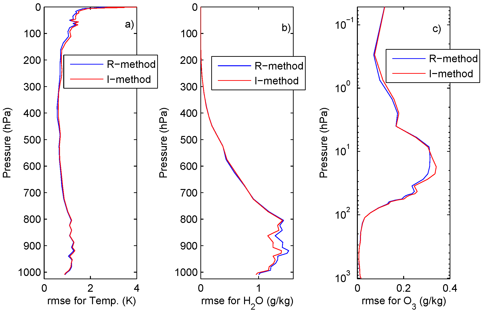
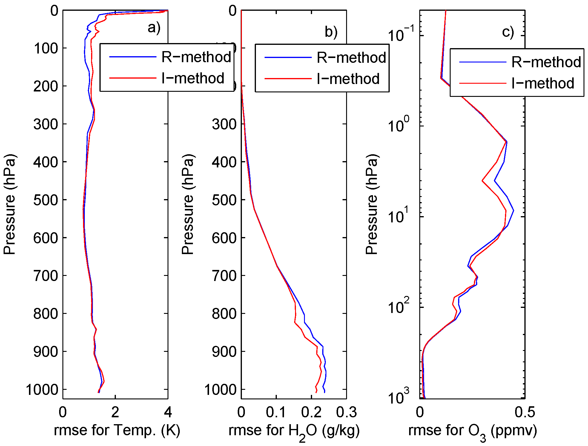
2.2. Forward and Inverse Modeling

Radiative transfer calculations have been performed with the package ϕ-IASI, which, among many others, incorporates a proper forward model, σ-IASI, and a linear regression inverse algorithm, that we call ε-IASI.

The scheme ϕ-IASI has been variously described in the science literature [9,11,14,15,16], which the reader is referred to for further details.

The σ-IASI forward module is a monochromatic radiative transfer model, which uses a suitable atmospheric layering method to model the optical depths. This consists of a grid of vertical slabs with constant pressure. Each layer is defined by the two bounding grid pressure levels (therefore N layers require a $N+1$ level grid). The discretized version of the radiative transfer equation, which is solved within σ-IASI, uses 63-layer pressure grid which spans the range $1100-0.005$ hPa.

Of course, monochromatic synthetic radiances are convolved with the appropriate IASI instrument spectral response function, to yield synthetic IASI spectra.

The retrieval scheme gets estimates of skin temperature, $T_s$, temperature profile, T, water vapour profile, w, and ozone profile, q. The profile are obtained on the same pressure grid used for forward calculations, therefore, $T,w,q$ are vectors of size 63 each.

The linear retrieval scheme adopts the principle of inverse regression, in which a given parameter, $y\left(p\right)$ at a given pressure layer, p is expressed as a linear function of a suitable number, r of PC scores.

$$y\left(p\right)-\overline{y}\left(p\right)={\beta }_1{c}_1+\cdots +{\beta }_r{c}_r$$

(6)

with $\overline{y}\left(p\right)$ the expectation value of $y\left(p\right)$, and where ${\beta }_i,i=1,\dots ,r$ are regression coefficients to be determined on the basis of, e.g., a suitable training data set. The PC scores, $c_i,i=1,\dots ,r$ can be obtained from the EOF transform of training spectra or interferograms. A detailed account of the EOF retrieval methodology can be found in [9,12]. The methodology has been developed for a generic signal-noise model and can be applied to any couple of data space and parameter space.

For completeness, we have to say something about the noise in the two data spaces: radiance and interferogram. For IASI we have a direct knowledge of the noise in the spectral domain, so that we need a suitable model, which transforms the noise between the two data spaces.

If we assume, as usual, a signal-noise model of a pure additive type

$$R_t\left(\sigma \right)=s_t\left(\sigma \right)+e\left(\sigma \right)$$

(7)

where $s_t\left(\sigma \right)$ is the signal, $e\left(\sigma \right)$ a noise term and $R_t\left(\sigma \right)$ the (noisy) observation. Then according to the basic Equation (3), which defines the interferogram, we have

$$I\left(x\right)={\int }_{-\infty }^{+\infty }(s_t\left(\sigma \right)+n\left(\sigma \right))exp(-2\pi i\sigma x)d\sigma$$

(8)

which says that the noise transforms the same way as the spectrum does.

The Fourier transform can be written in terms of a suitable matrix, $\mathbf{F}$ so that Equation 8 can be written in vector form (e.g., see [17]),

$$\mathbf{I}=\mathbf{F}{\mathbf{s}}_t+\mathbf{F}\mathbf{e}$$

(9)

where $\mathbf{I},{\mathbf{s}}_t,\mathbf{e}$ are the interferogram signal and noise vectors. Then, if ${\mathbf{C}}_e$ is the covariance matrix of the spectral noise term, the corresponding covariance matrix, ${\mathbf{C}}_n$ in the interferogram domain is easily obtained by the linear transform

$${\mathbf{C}}_n=\mathbf{F}{\mathbf{C}}_e{\mathbf{F}}^t$$

(10)

where ${\mathbf{F}}^t$ is the transpose of the matrix $\mathbf{F}$.

In the work here shown the noise in the spectral domain is assumed to have variance according to the level 1C IASI noise, and the corresponding noise strength in the interferogram domain is calculated according to Equation (10).

3. Data Reduction Applied to IASI

Exploiting the methodology outlined in section 2.1, in this section suitable data reductions for IASI are shown and described, which are based on truncating the IASI interferogram at points below its maximum path difference of 2 cm. The interferogram-based data reduction will be compared to that usually performed in the spectral domain by picking up sparse channels, on the basis, e.g., of minimum-loss information criterions (see e.g., [4]).

To avoid possible confusion and misunderstanding, we will henceforth refer to as

• I-method, the method which is based on the truncation of the interferogram at point below the IASI maximum path difference of 2 cm,
• R-method, the method which is based on the selection of sparse spectral channels from the IASI spectrum at its nominal sampling $\Delta \sigma =0.25$ cm${}^{-1}$.

Figure 4. Example of IASI spectrum, $R\left(\sigma \right)$, with the indication of the 3,385 selected for the R-method.

Figure 4. Example of IASI spectrum, $R\left(\sigma \right)$, with the indication of the 3,385 selected for the R-method.

We consider two subsets of reduced IASI data. For the first case the 8461 IASI channels are reduced of a factor 2.5, whereas for the second case of a factor $\approx 30$.

It should be also stressed that, for the case of the R-method, the reduction of data points completely destroys the original IASI spectral coverage, whereas in the case of the I-method, the truncation provides a sinc-interpolation of the original data, which leaves unchanged the full IASI spectral coverage.

3.1. Data Reduction of a Factor 2.5

For this first case, the I-method considers a truncation point $x_t=0.8$ cm, which corresponds to $N=3385$ data points. This moderate data-reduction allows us to retain the first CO${}_2$ signature in the interferogram domain (see Figure 1) and is equivalent to work with a spectrum with the full IASI spectral coverage, but a sampling $\Delta \sigma =0.625$ cm${}^{-1}$, instead of the original 0.25 cm${}^{-1}$ (see e.g., Figure 2).

The R-method considers the IASI spectrum at its nominal sampling rate, $\Delta \sigma =0.25$ cm${}^{-1}$, therefore we preserve the original IASI spectral resolution, but we select a set of $N=3385$ channels. These channels are exemplified in Figure 4 and belong to spectral ranges which include

• the ${\nu }_2$ absorption band of CO${}_2$ and part of the atmospheric window (range from 645 to 830 cm${}^{-1}$)
• the ozone band at 9.6 μm
• the atmospheric window from 1,100 to 1,200 cm${}^{-1}$
• the core of the ${\nu }_2$ absorption band of H${}_2$O at 6.7 μm
• the portion of the spectrum from 2,000 to 2,230 cm${}^{-1}$, this includes a part of the N${}_2$O/CO${}_2$ absorption band at 4.3 μm

We stress that the spectral ranges considered yield 3385 spectral channels, therefore, we have exactly the same data points as those for the I-method. The channels we have selected are a trade-off between the need to limit the data volume and to preserve portions of the spectrum which are mostly sensitive for the retrieval of temperature, water vapour and ozone. In particular we do not include the spectral segments

• 810 to 1,000 cm${}^{-1}$ because of unknown contamination from CFC absorption;
• 1,200 to 1,450 because of strong contamination by CH${}_4$;
• 2,230 to 2,760, because of spectroscopic issues such as CO${}_2$ line and continuum absorption uncertainty, e.g., [16], non LTE effects and sun contribution during the day.

3.2. Data Reduction of a Factor $\approx 30$

The R-method considers exactly the same 300 IASI channels as those selected in [4]. These channels are those routinely monitored at ECMWF. These include the 168 IASI spectral channels, which are effectively assimilated at ECMWF [2]. The 300 channels are shown in Figure 5 and they were selected to optimize information content for temperature, water vapour and ozone. These channels also include a set of 44 short wave channels (IASI band 3), which during the day are affected by solar energy. They were intended for night observations, and should not be used for day time IASI soundings.

However, in this study they will be purposely used also for daytime IASI spectra to be contrasted and compared to the truncation-interferogram approach, in order to show and demonstrate how the I-method is largely insensitive to the day-night cycle.

This channel selection will be compared to the truncation point of $x_t=0.0701$ cm, which yields $N=300$ interferogram data points.

Figure 5. (a) Example of IASI spectrum, $R\left(\sigma \right)$, with the indication of the 300 IASI channels routinely monitored at ECMWF and (b) interferogram truncated at $x_t=0.0701$ cm in such a way to retain only 300 interferogram data points.

Figure 5. (a) Example of IASI spectrum, $R\left(\sigma \right)$, with the indication of the 300 IASI channels routinely monitored at ECMWF and (b) interferogram truncated at $x_t=0.0701$ cm in such a way to retain only 300 interferogram data points.

4. Results: Assessment of the Retrieval Capability of the I-method and R-method

As anticipated the data reduction strategies are intended for near real time dissemination and processing of IASI data for the retrieval of temperature, water vapour and ozone.

In this section, an evaluation of the subsets of IASI channels as far as the retrieval performance is concerned will be performed.

The evaluation will be carried out on the basis of the parametric, statistical retrieval scheme, which has been discussed in section 2.2. A statistical retrieval methodology has been used, mostly because of its simplicity of implementation, which alleviate the computational burden in view of the many cases we are going to analyze. We are mostly interested in performing a comparison between the R-method and the I-method. Although the retrieval performance could depend on the inversion algorithm, the retrieval performance difference between the R-method and the I-method is independent of the retrieval scheme, since it depends on the information content of spectral radiances or interferometric radiances for temperature, water vapour and ozone.

We stress, that for the R-method the data space is a suitable set of spectral radiances, which are selected at specific spectral ranges in order to maximize the sensitivity to the retrieved parameters, $(T_s,T,w,q)$, and, possibly, minimize the effect of interfering parameters, such as trace gas species. For the purpose of retrieval, the set of channels is further EOF transformed to reduce the dimensionality of the inverse problem.

For the I-method the data space is constituted by interferometric radiances in the range $[0,x_t]$, where $x_t$ is a suitable truncation point, which according to Section 3 can assume the values 0.8 cm and 0.0701 cm, respectively. The truncation at the optical path difference, $x_t$ corresponds to spectra with a sampling $\Delta \sigma ={\left(2x_t\right)}^{-1}$. Also in this case, the truncated interferogram is further EOF transformed to reduce the dimensionality of the inverse problem.

4.1. A Case Study in Simulation

First we discuss a case obtained in simulation and begin with presenting the results for ($N=3385$, $x_t=0.8$ cm).

The case study is obtained by considering a set of atmospheric state vectors for $T_s,T,w,q$ selected from the Chevalier data base [18]. The set consists of 377 sea-surface, clear-sky, tropical profiles for the parameters $T_s,T,w,q$. The set was used to yield IASI pairs $\left(R\right(\sigma ),I(x)$), which once properly added with noise were processed to retrieve the atmospheric parameters.

This exercise provides a case for which the true state of the atmosphere is perfectly known and there are no forward and spectroscopic biases, but only random observational noise.

For the case of the skin temperature both methods give a very high performance: the root mean square error is equal to 0.06 K.

The results for the temperature retrieval performance is shown in Figure 6(a). It is seen that the two methods give equivalent results for temperature and perform quite well. Note that this is the best performance we can achieve because we are performing the retrieval exercise in simulation, in which we assume a perfect world. For this case, the R-method brings information about temperature from the longwave absorption band of CO${}_2$ and from the shortwave segment 2,000 to 2,230 cm${}^{-1}$. We are simulating no biases because of sunlight or non LTE effects.

Figure 6. Results for the case study in simulation and for ($N=3385$, $x_t=0.8$ cm). The figure shows the retrieval performance expressed in terms of root mean square error (rmse) for (a) temperature, (b) water vapour and (c) ozone.

Figure 6. Results for the case study in simulation and for ($N=3385$, $x_t=0.8$ cm). The figure shows the retrieval performance expressed in terms of root mean square error (rmse) for (a) temperature, (b) water vapour and (c) ozone.

For water vapour the retrieval performance is shown in Figure 6(b). It is seen that now the I-method provides a slight but consistent better retrieval in the lower atmosphere, where the water vapour has the larger variability. We think that this finding can be explained because of the better representation of H${}_2$O continuum and line absorption within the I-method than the R-method. In fact, while the R-method does not take into account for the full spectral coverage of IASI (see Figure 4), the I-method does.

Finally, for ozone the retrieval performance is shown in Figure 6(c). The ozone band is very well insulated in the middle of the spectral coverage (see Figure 4) and adds a sensible contribution to the total energy, so that its signature is strong in both domains. As a result the R-method and the I-method yield almost the same results, with a slight advantage for the R-method.

The results just illustrated says that in case the number of IASI data remains relatively large and of the same order of $N_{IASI}$, the two methods are almost equivalent, although the I-method is slightly superior for the retrieval of lower atmospheric moisture, which is a primary objective of IASI.

The superiority of the I-method is largely enhanced in case we ask for a larger data-reduction, as we will show discussing the same exercise as that above, but for the case ($N=300$, $x_t=0.0701$ cm).

The results for the temperature retrieval performance is shown in Figure 7(a). It is seen that the R-method is superior over the I-method in the upper part of the atmosphere. Conversely, in the lower troposphere, the I-method performs better than the R-method. If we consider the case of water vapour, whose retrieval accuracy is shown in Figure 7(b), we see that the I-method outperforms in the lower atmosphere the R-method. Once again, we think that this finding can be explained because of the best spectral coverage, and the effect is here much more evident than for the case shown in Figure 6, since now the density of the 300 full spectral resolution IASI channels is very low within the ${\nu }_2$ band of H${}_2$O (see e.g., Figure 5).

For ozone, the channel density within the band at 9.6 μm is even smaller, and as a result the I-method yields a better performance than the R-method (see Figure 7(c)).

Figure 7. Results for the case study in simulation and for ($N=300$, $x_t=0.0701$ cm). The figure shows the retrieval performance expressed in terms of root mean square error (rmse) for (a) temperature, (b) water vapour and (c) ozone.

Figure 7. Results for the case study in simulation and for ($N=300$, $x_t=0.0701$ cm). The figure shows the retrieval performance expressed in terms of root mean square error (rmse) for (a) temperature, (b) water vapour and (c) ozone.

The superiority of the I-method is confirmed also in case we consider high-latitude, cold air masses. In this respect, since the I-method is expected to have a better signal-to-noise, it should be promising for application, especially for processing IASI data at high and/or middle latitude geographic areas in winter season.

Figure 8 compares the retrieval performance of the I-method to that of the R-method for a case of high-latitude-winter IASI soundings. As for the tropical exercise, this set of soundings was built up by considering a suitable ensemble of atmospheric state vectors extracted from the Chevalier data base [18]. The ensemble consists of 138 clear-sky, high-latitude-winter profiles for the parameters $T_s,T,w,q$. The set was used to yield IASI pairs $\left(R\right(\sigma ),I(x)$), which once properly added with noise were processed to retrieve the atmospheric parameters.

For the sake of brevity the analysis is here limited to the case ($N=300$, $x_t=0.0701$ cm). It is seen from Figure 8 that the comparison of the I-method against the R-method for this case of a cold atmosphere closely parallels the comparison results presented in Figure 7 for a hot, tropical atmosphere. Temperature retrieval performance is nearly the same for the two methods in the troposphere, whereas for water vapour and ozone the performance provided by the I-method is superior of that of the R-method.

4.2. The JAIVEx Case Study

As for the previous paragraph, we begin with discussing the results for the data-reduction of ($N=3385$, $x_t=0.8$ cm).

The Joint Airborne IASI validation experiment (JAIVEx) [19] was carried over the Gulf of Mexico during April and May 2007. We have a series of 6 spectra for the day 29 April 2007, 16 spectra for the day 30 April 2007, and finally 3 spectra for the day 4 May 2007. The total of 25 soundings are time and space colocated with dropsonde observations. The dropsonde analysis extends from the ground level to about 400 hPa, therefore the atmospheric profiles have been extended up to 0.1 hPa through the analysis of the ECMWF.

Figure 8. Results for the case study in simulation and for ($N=300$, $x_t=0.0701$ cm). The figure shows the retrieval performance expressed in terms of root mean square error (rmse) for (a) temperature, (b) water vapour and (c) ozone. The results applies to high-latitude-winter IASI soundings.

Figure 8. Results for the case study in simulation and for ($N=300$, $x_t=0.0701$ cm). The figure shows the retrieval performance expressed in terms of root mean square error (rmse) for (a) temperature, (b) water vapour and (c) ozone. The results applies to high-latitude-winter IASI soundings.

The JAIVEx observations were taken during daytime, therefore they also allows us to assess the robustness of the two retrieval methods to the solar contamination in the short wave side of the spectrum. Note that our radiative transfer calculations does not purposely include the solar term to assess its potential interfering effect over retrievals.

In addition, the real data from the JAIVEx campaign allows us to understand the sensitivity of the two methods to the interfering effect of trace gases, which in our radiative calculations are kept constant to their climatological values. Particularly relevant to our analysis are the potential effect due to the variability of CH${}_4$ and CO. Note that the effect of both CH${}_4$ and CO have to be expected for the I-method, which uses the full IASI spectral coverage. For the case of the R-method the methane band has been eliminated form the selected ranges (again see Figure 4), while the CO band has been included.

Keeping this in mind, Figure 9 summarizes the root mean square error for temperature, water vapour and ozone. When comparing the results shown in Figure 9 to those in Figure 6 it has to be considered that the findings for the JAIVEx experiment are based only on 25 soundings.

For temperature and ozone the two approaches gives almost the same results, while the I-method is superior over the R-method for water vapour in the lower part of the atmosphere. It is also important to note that while for the R-method we selected suitable ranges in order to minimize the interfering effects of the sun in the short wave and that of CH${}_4$ in the left wing of the water vapour band at 6.7 μm, none of this precautions were taken for the I-method, which just consider the full spectral coverage.

The results for H${}_2$O is important and deserves further analysis to get insight into understanding whether the improvement involves only the root mean square or the spatial vertical resolution of the profile itself.

Towards this objective Figure 10 compare the retrieved H${}_2$O-profiles to the dropsonde observations for the day 29 April 2007. It is interesting to note that the I-method is capable to resolve the double layer structure which is seen in the lower part of the water vapour profiles. This is done much better than the

Figure 9. Results for the JAIVEx case study and the case ($N=3385$, $x_t=0.8$ cm). The figure shows the retrieval performance expressed in terms of root mean square error (rmse) for (a) temperature, (b) water vapour and (c) ozone.

Figure 9. Results for the JAIVEx case study and the case ($N=3385$, $x_t=0.8$ cm). The figure shows the retrieval performance expressed in terms of root mean square error (rmse) for (a) temperature, (b) water vapour and (c) ozone.

Figure 10. Results for the JAIVEx case study and for the case ($N=3385$, $x_t=0.8$ cm). Day 29 April 2007. The figure shows the mean retrieved profile for H${}_2$O for the two retrieval approaches and their comparison with the dropsonde observation. The retrieved profile has been averaged over the six available IASI soundings.

Figure 10. Results for the JAIVEx case study and for the case ($N=3385$, $x_t=0.8$ cm). Day 29 April 2007. The figure shows the mean retrieved profile for H${}_2$O for the two retrieval approaches and their comparison with the dropsonde observation. The retrieved profile has been averaged over the six available IASI soundings.

R-method, which, conversely, barely sees the water vapour feature in the lower atmosphere. This means that the I-method provides results, which are better vertically resolved in comparison to the R-method.

This is confirmed also from the results for the two remaining days, which are not shown here for the sake of brevity. It is much more interesting to compare this result for H${}_2$O to that obtained with ($N=300$, $x_t=0.0701$ cm), which is shown in Figure 11.

Also for this case, the I-method is capable to resolve the double layer structure which is seen in the lower part of the water vapour profiles. Again, this is done much better than the R-method.

Especially for the case of the I-method, comparing the results shown in Figure 10 to those in Figure 11 it seems that we are faced with a situation in which the lesser the number of data, the better the results.

We think that this is in part the effect of limiting the impact of interfering factors when we move the truncation point close the origin, since we move in a region with a better signal-to-noise ratio. This

Figure 11. Results for the JAIVEx case study and for the case ($N=300$, $x_t=0.0701$ cm). Day 29 April 2007. The figure shows the mean retrieved profile for H${}_2$O for the two retrieval approaches and their comparison with the dropsonde observation. The retrieved profile has been averaged over the six available IASI soundings.

Figure 11. Results for the JAIVEx case study and for the case ($N=300$, $x_t=0.0701$ cm). Day 29 April 2007. The figure shows the mean retrieved profile for H${}_2$O for the two retrieval approaches and their comparison with the dropsonde observation. The retrieved profile has been averaged over the six available IASI soundings.

has also the effect that more EOF scores go above the noise level for $x_t=0.0701$ cm than with $x_t=0.8$ cm. If we increase the number of EOF scores in the retrieval scheme, we add more degrees of freedom, hence information to the regression analysis, which improves the spatial vertical resolution. However, this results has to be more carefully assessed on the basis of more extensive set of IASI soundings.

The results shown in Figure 10 to those in Figure 11 also suggest that there should be an optimal truncation point, which minimizes the root mean square error for H${}_2$O. An issue that we plan to investigate in a future study.

Figure 12 and Figure 13 provide a case for temperature, for the two different strategies ($N=3385$, $x_t=0.8$ cm) and ($N=300$, $x_t=0.0701$ cm), respectively, which further deserves to exemplify the better capability of the I-method to capture fine structures also in the temperature profile. It is seen from these two figures that the I-method resolves better than the R-method the temperature inversion at about 800 hPa, and also the details in the upper troposphere at about 200 hPa are captured much better.

It is also very much interesting to note the bad performance of the R-method for the case of the temperature retrieval shown in Figure 13. This is due to the sensitivity of 44 out of the 300 IASI channels to the short-wave side of the spectrum (see Figure 5). These channels were purposely included to show that the I-method, unlike the R-method, is insensitive to the interfering effects of the solar energy.

When we remove the 44 short-wave IASI channels, the R-method gets comparable results to those of the I-method. However, the performance for water vapour remains below that of the I-method.

To sum up we can say that the I-method provides better results for the retrieval of water vapour, and also for temperature it seems to capture better fine details. Furthermore, the I-method is fairly insensitive to the potential interfering effects of solar energy and radiatively active trace gases. This simplifies a lot the radiative transfer calculation and avoids the computational burden of including the solar source in the computations.

Figure 12. Results for the JAIVEx case study and for ($N=3385$, $x_t=0.8$ cm). Day 30 April 2007. The figure shows the mean retrieved profile for temperature for the two retrieval approaches and their comparison with the dropsonde observation. The retrieved profile has been averaged over the 16 available IASI soundings.

Figure 12. Results for the JAIVEx case study and for ($N=3385$, $x_t=0.8$ cm). Day 30 April 2007. The figure shows the mean retrieved profile for temperature for the two retrieval approaches and their comparison with the dropsonde observation. The retrieved profile has been averaged over the 16 available IASI soundings.

4.3. The Tropical Case Study

To boost the results obtained in the previous section with a better statistics we consider a second data set of IASI spectra, which has been acquired within the tropical belt, during the IASI commissioning phase on 22 July 2007. In total, a number of 647 IASI spectra has been selected. The spectra have been observed on sea surface and refer to nadir looking mode and clear sky conditions. Clear sky was checked using the cloud detection scheme described in [15]. This second set of data will be referred to as simply the tropical set.

For the tropical set, in order to develop a consistent set of truth data against which IASI retrieval could be compared, ECMWF atmospheric analysis fields for temperature, water vapor and ozone were considered. These fields where time and spatially co-located to the 647 IASI soundings. We used atmospheric analysis fields of 00:00, 06:00, 12:00, 18:00 and 24:00 UTC on 22 July 2007. For more details we refer the reader to [16].

The tropical set is made up of 87 daytime IASI spectra, whereas the remaining 560 spectra have been observed during the night. To exemplify the robustness of the I-method to the interfering effect of solar energy, in the following the statistics will be separately shown for day and night conditions.

Figure 14 summarizes the performance of the two approaches for ($N=3385$, $x_t=0.8$ cm). In this case the root mean square difference is also influenced by the statistical accuracy of the ECMWF analysis itself, which in the troposphere is about $\pm 1$ K for temperature and $\approx \pm 0.5$ g/kg for water vapour [16]. For this reason we have to expect a relatively larger root mean square difference than that shown in the two previous sections. The results shown in Figure 14 confirm that the I-method yields a retrieval performance for water vapour that is superior to that obtained with the R-method. In general, the results say that the I-method provides a better accuracy also for the case of temperature, in the lower troposphere, and almost everywhere for ozone.

In daytime the I-method outperforms the R-method also for the case of temperature, mainly because the latter is more sensitive than the former to solar effects in the IASI band 3. Although the R-method,

Figure 13. Results for the JAIVEx case study and for ($N=300$, $x_t=0.0701$ cm). Day 30 April 2007. The figure shows the mean retrieved profile for temperature for the two retrieval approaches and their comparison with the dropsonde observation. The retrieved profile has been averaged over the 16 available IASI soundings.

Figure 13. Results for the JAIVEx case study and for ($N=300$, $x_t=0.0701$ cm). Day 30 April 2007. The figure shows the mean retrieved profile for temperature for the two retrieval approaches and their comparison with the dropsonde observation. The retrieved profile has been averaged over the 16 available IASI soundings.

for the case ($N=3385$, $x_t=0.8$ cm), has its farer channel at 2230 cm${}^{-1}$, some contamination from sun energy has to be expected, mostly for the spectral segment 2100 to 2200 cm${}^{-1}$. Another interfering effect in this band is CO absorption.

In nighttime the two methods yield almost the same results, although the I-method still seems to produce a better performance in the lower troposphere, both for temperature and water vapour.

Form Figure 14 it appears that the retrieval performance depends on the day/night cycle. We think that this is only an effect of the different statistics, 87 cases for daytime against 560 for nighttime.

Similar results to those we have just discussed and shown in Figure 14 are achieved by considering (see Figure 15) the case ($N=300$, $x_t=0.0701$ cm). Now the negative effect of the solar contamination is most evident for the R-method, which again gives more evidence to the fact the I-method has a low sensitivity to the contamination by infrared emission of the sun.

As for the case ($N=3385$, $x_t=0.8$ cm), we see a dependence on the day/night cycle and on overall we obtain results, which are in agreement with those shown in Figure 14.

Finally, we also stress that if for daytime we do not use the 44 short-wave channels in order to limit solar contamination, the performance of the R-method improves, but it remains inferior to that obtained with the I-method. This is exemplified for water vapour in Figure 16. Similar results holds for temperature and ozone.

Figure 14. Results for the tropical case study for ($N=3385$, $x_t=0.8$ cm). The figure shows the retrieval performance expressed in terms of root mean square error (rmse) for (a) temperature, (b) water vapour and (c) ozone.

Figure 14. Results for the tropical case study for ($N=3385$, $x_t=0.8$ cm). The figure shows the retrieval performance expressed in terms of root mean square error (rmse) for (a) temperature, (b) water vapour and (c) ozone.

Figure 15. Results for the tropical case study for ($N=300$, $x_t=0.0701$ cm). The figure shows the retrieval performance expressed in terms of root mean square error (rmse) for (a) temperature, (b) water vapour and (c) ozone.

Figure 15. Results for the tropical case study for ($N=300$, $x_t=0.0701$ cm). The figure shows the retrieval performance expressed in terms of root mean square error (rmse) for (a) temperature, (b) water vapour and (c) ozone.

5. Discussion and Conclusions

The study has been mostly focused on the application to IASI of data reduction strategies complemented with a statistical regression methodology, which is able to work indifferently with spectral radiances or interferogram samples. Different data-reduction approaches, yielding a number, N of spectral radiances, with N in the range $N\le N_{IASI}$ and $N<<N_{IASI}$, respectively, have been studied and inter-compared in order to assess their relative retrieval performance.

Based on a series of retrieval exercises, we have shown that the interferogram-truncation approach provides a suitable data-reduction methodology in all those cases we are constrained by $N<<N_{IASI}$ and we are interested in the retrieval of temperature and water vapour. In fact, irrespectively of the point at which we truncate the interferogram, the I-method preserves the IASI spectral coverage. This is important for water vapour, which is radiatevely active across the full IASI spectral coverage.

Figure 16. Results for the tropical case study and for daytime IASI soundings. The figure shows the retrieval performance expressed in terms of root mean square error (rmse) for water vapour and compares the I-method to the R-method with and without solar channels. The results shown in figure applies to the case ($N=300$, $x_t=0.0701$ cm).

Figure 16. Results for the tropical case study and for daytime IASI soundings. The figure shows the retrieval performance expressed in terms of root mean square error (rmse) for water vapour and compares the I-method to the R-method with and without solar channels. The results shown in figure applies to the case ($N=300$, $x_t=0.0701$ cm).

It could be argued that in the interferogram domain temperature and water vapour are deeply convolved, while in the spectral domain we can achieve a separation of the absorption bands, in such way to insulate temperature channels from those of water vapour. However, because of the water vapour continuum absorption, there is no part of the spectrum which is really not influenced by water vapour, and the effect of H${}_2$O becomes increasingly important and convolved with temperature when we consider spectral channels, which peak deeply in the troposphere, which, in turn, is the part of the atmosphere mostly relevant to meteorological processes. Thus, in both spaces, there is no way to really insulate temperature from water vapour. There could be also some constraints, which are determined, e.g., from the kind of retrieval process one uses to invert atmospheric parameters from radiances (e.g., the need of well shaped Jacobian and/or averaging kernels). These constraints appear to be of mathematical nature rather than of physical meaning. However, it is fair to say that the capability of the interferogram approach has to be confirmed and better assessed also with the use of physical inversion of the radiative transfer equation performed into the interferogram domain, which means, e.g., the computation of derivative of $I\left(x\right)$ with respect to parameters such as $T,w,q$.

Having said that, it is important to stress that our results demonstrate that the retrieval capability of the interferogram domain has been largely under-explored until now, which call for a more comprehensive analysis, especially in the quest of suitable methods to reduce the size of IASI data to be transmitted and processed.

In perspective, once we recognize that FTS instruments measure the interferogram, we could then make a direct use of interferometric radiances that could allows us to deal with fairly constant-variance and uncorrelated noise, which would further improve the quality and independency of data and, hence, retrievals, and finally could even simplify the design of future satellite instrumentation.

References and Notes

1. Richter, A.; Wagner, T. The IASI instrument onboard the METOP Satellite: First results. Atmos. Chem. Phys. 2009. Special Issue. Available online: http://www.atmos-chem-phys.net/special_issue123.html (accessed on 29 September 2010).
2. Collard, A.D.; McNally, A.P. The assimilation of Infrared Atmospheric Sounding Interferometer radiances at ECMWF. Q. J. R. Meteorol. Soc. 2009, 135, 1044–1058. [Google Scholar] [CrossRef]
3. Robinson, E.A.; Silvia, M.T. Digital Foundation of Time Series Analysis: Wave-Equation Space-Time Processing; Holden-Day: San Francisco, CA, USA, 1981; Volume 2. [Google Scholar]
4. Collard, A.D. Selection of IASI channels for use in numerical weather prediction: The assimilation of Infrared Atmospheric Sounding Interferometer radiances at ECMWF. Q. J. R. Meteorol. Soc. 2007, 133, 1977–1991. [Google Scholar] [CrossRef]
5. Kaplan, L.D.; Chahine, M.T.; Susskind, J.; Searle, L.E. Spectral band passes for a high precision satellite sounder. Appl. Opt. 1977, 16, 322–325. [Google Scholar] [CrossRef] [PubMed]
6. Kyle, T.G. Temperature soundings with partially scanned interferograms. Appl. Opt. 1977, 16, 326–333. [Google Scholar] [CrossRef] [PubMed]
7. Smith, W.L.; Howell, H.B.; Woolf, H.M. The use of interferometric radiance measurements for the sounding the atmosphere. Appl. Opt. 1979, 36, 566–575. [Google Scholar]
8. Huang, H.-L.; Antonelli, P. Application of principal component analysis to high- resolution infrared measurements compression and retrieval. J. Appl. Metereo. 2001, 40, 365–388. [Google Scholar]
9. Serio, C.; Masiello, G.; Grieco, C. EOF regression analytical model with applications to the retrieval of atmospheric temperature and gas constituents concentration from high spectral resolution infrared observations. In Environmental Modelling: New Research; Findley, P.N., Ed.; Nova Science Publishers, Inc.: Hauppagauge, NY, USA, 2009; pp. 51–88. [Google Scholar]
10. Goldberg, M.D.; Qu, Y.; McMillin, L.M.; Wolf, W.; Zhou, L.; Divakarla, M. AIRS near-real-time products and algorithms in support of operational numerical weather prediction. IEEE Trans. Geosci. Remote Sens. 2003, 41, 379–389. [Google Scholar] [CrossRef]
11. Masiello, G.; Serio, C. Dimensionality-reduction approach to the thermal radiative transfer equation inverse problem. Geophys. Res. Lett. 2004, 31, L11105. [Google Scholar] [CrossRef]
12. Serio, C.; Esposito, F.; Masiello, G.; Pavese, G.; Calvello, M.R.; Grieco, G.; Cuomo, V.; Buijs, H.L.; Roy, C.B. Interferometer for ground-based observations of emitted spectral radiance from the troposphere: evaluation and retrieval performance. Appl. Opt. 2008, 47, 3909–3919. [Google Scholar] [PubMed]
13. Zhou, D.K.; Smith, W.L.; Li, J.; Howell, H.B.; Cantwell, G.W.; Larar, A.M.; Knuteson, R.O.; Tobin, D.C.; Revercomb, H.E.; Bingham, G.E.; Tsou, J-.J.; Mango, S.A. Thermodynamic product retrieval methodology and validation for NAST-I. Appl. Opt. 2002, 41, 6957–6970. [Google Scholar] [CrossRef] [PubMed]
14. Amato, U.; Masiello, G.; Serio, C.; Viggiano, M. The σ-IASI code for the calculation of infrared atmospheric radiance and its derivatives. Environ. Model. Software 2002, 17, 651–667. [Google Scholar] [CrossRef]
15. Grieco, G.; Masiello, G.; Matricardi, M.; Serio, C.; Summa, D.; and Cuomo, V. Demonstration and validation of the φ-IASI inversion scheme with NAST-I data. Q. J. R. Meteorol. Soc. 2007, 133, 217–232. [Google Scholar] [CrossRef]
16. Masiello, G.; Serio, C.; Carissimo, A.; Grieco, G. Application of ϕ-IASI to IASI: Retrieval products evaluation and radiative transfer consistency. Atmos. Chem. Phys. 2009, 9, 8771–8783. [Google Scholar] [CrossRef]
17. Amato, U.; De Canditiis, D.; Serio, C. Effect of apodization on the retrieval of geophysical parameters from Fourier-Transform Spectrometers. Appl. Opt. 1998, 37, 6537–6543. [Google Scholar] [CrossRef] [PubMed]
18. Chevalier, F. Sampled Database of 60 Levels Atmospheric Profiles from the ECMWF Analysis; Technical Report; ECMWF EUMETSAT SAF programme Research Report 4; ECMWF: Shinfield Park, Reading, UK, 2001. [Google Scholar]
19. Taylor, J.P. Joint Airborne IASI Validation Experiment. Available online: http://badc.nerc.ac.uk/data/jaivex/ (accessed on 29 September 2010).