Development and Evaluation of Phenological Change Indices Derived from Time Series of Image Data

Abstract

Changes in vegetation phenology are recognized as being possibly the most important early indicator of the impact of climate change on ecosystems. Time series of image data are accepted as being the best way to map these changes, if we can derive suitable indices from the huge volumes of time series data that make the interpretation of these time series difficult. The problem is thus to derive a set of indices from the time series of image data that depict changes in vegetation phenology in a way that is easy to analyze and use.

This problem has been solved by deriving a set of six Phenological Change Indices that measure the five ways that the phenological curve of vegetation can change over time. These indices were then tested using simulated data based on sample phenological profiles for a set of land covers and showed that four of the indices measured four of the ways that the phenological profile can change, and two of the indices gave similar results in measuring the last way that the phenological profiles can change.

A time series of image data was then used to map the Phenological Change Indices for Eurasia and a sample of land covers was used to relate the changes in phenology to location for each land cover. This work showed that the detected changes in phenology are similar to those found in other papers. The benefit of these indices is that we can now analyze changes in phenology in a much more detailed and accurate way than has been possible until now.

1. Background

Phenology is defined as “the study of the timing of recurring biological events, the causes of their timing with regard to biotic and abiotic forces, and the interrelationship among phases of the same or different species” [1]. In this paper Phenological Cycle is defined as the trace or record of the changes in a variable or attribute over the phenological period (usually one year) and a phenophase is defined as an observable stage or phase in the seasonal cycle of a plant that can be defined by start and end points [2].

Climate is one of the dominant drivers for vegetative growth and dieback and as a consequence, changes in climate are likely to induce changes in vegetation phenophases. Changes in phenophase timing have been identified as being perhaps the simplest way to track changes in the ecosystem composition and functioning in response to climate change [3]. Phenology is also deemed to be important because changes in phenology often have cascading effects on other properties of the ecosystem. Thus, for example, a longer growing season can affect surface evapo-transpiration, albedo, carbon fixation and nutrient cycling both at a particular time and integrated over a season [3].

There is a large body of evidence that shows that many species from many different parts of the globe are changing their phenology. Extensive German phenological data for the period 1951–1996 was analyzed by [4], revealing that there are clear advances in the time of both the earliest and early spring phenophases, and notable advances in the succeeding spring phenophases, such as the leaf unfolding of deciduous tree species. Menzel et al. [4] found that the phenophase timing changes are less pronounced in autumn, but that despite the difficulty of measuring the end of season, there is clear evidence of lengthening of the growing season. Phenological data recording six major phenophases for 29 species in Spain over the period 1943–2003 were investigated by [5], who found that the vast majority of these phenophases underwent a shift in their dates since the mid 1970’s. Leaf unfolding, flowering and fruiting were found to be markedly advancing in some species, but not in others. For example they found that wind pollinated plant species have advanced their flowering more than insect and animal pollinated plants. Many others have found corroborating results as summarized in [3].

Some of this work has linked these changes to key climate parameters including temperature, rainfall and humidity, showing that the greenup of different plant communities can be dominated by different climate parameters, further complicating any analysis. For example the onset of greenup in Spain changes from spring, in the northern cooler climate areas where this phase is triggered by temperature, to autumn in the south where this event is triggered by rainfall [6]. They report that rainfall and water availability can cause complex phenological changes, with far-reaching consequences for ecosystem functioning and structure. Others have shown that water pulses prompt different responses from different species depending on the timing of the event relative to a given phenophase, rooting depth, and plant structural type [7]. They found that xerophytic plants responded more rapidly to the pulse than mesophytic plants. Others have found [8] that changes in the onset of spring are highly correlated with changes in temperature in Wisconsin, USA, a finding corroborated by [9] for a variety of agricultural crops.

While earlier onset of spring phenophases is highly correlated with changes in either temperature or rainfall, delays in autumn phenophases are less clear-cut. The usual explanation for this is that autumn events are often strongly influenced by other climatic and environmental processes such as the availability of soil moisture and humidity and the accumulated effects of seasonal events. It has been shown [10,11,12] that trees and grasses in the dry tropics often use water from different pedological horizons and, as a consequence, some species can have different phenological responses after the close of the wet season. This is further complicated by the adoption of different strategies for dealing with moisture stress by different species. For example Ziziphus mauritiana and Acacia senegal are categorized as being deciduous species which have a vegetative phase that coincides with that of the herbaceous layer, whilst other species such as Balanites aegyptiaca are evergreen with new growth phenophases occurring earlier than for the herbaceous layer and the level of green leaf only becoming low due to the presence of predators [10].

These processes are likely to explain the variation in temporal responses of different species noted by [5] who have reported that the existing calendar guilds of plants (or associations of plants that exhibit similar phenophase timing) are changing, causing changes in the inter-specific relationships between plants in the Iberian ecosystems. Similarly [13] found that species respond differently to climate change with the tendency for ecological communities to become disaggregated as the various species go out of synchronization. This has significant potential implications for interdependent relationships between species and for species composition in those ecosystems [14].

Plants (and animals) can reproduce, grow and survive within specific ranges of climatic and environmental conditions [3]. If conditions change beyond the tolerance of a species then it may respond by:

• Shifting the timing of life cycle events;
• Shifting range boundaries resulting in areas of extirpation and colonization;
• Changing morphology, reproduction or genetics; or
• Extinction.

All of these processes will lead to changes in the phenological profile of an ecosystem as the mix of species changes, or as individual species adapt to the changing climatic conditions. It has been noted that some of these changes do not happen gradually, leading to abrupt changes in ecosystem functions and species composition [6]. It is particularly important to identify areas that are changing abruptly because such change creates problems in developing appropriate management responses within the time available.

As has been noted, ground based phenological studies usually record the time at which key phenophases occur in individual species. This sort of information is not available from remotely sensed data. A remotely sensed image records the aggregated radiance at a specific moment for each picture element (pixel) in the population of pixels that constitute the whole image. Each pixel represents the integrated response across its field of view at a specific time. Since a diverse population of plants will occur within each pixel area, the record is an integration of the contribution from all of the plants and the background within this pixel area at that time [15]. This problem worsens as the species and/or community mix increases in the pixels, as is often the case with larger pixels.

The images that are used to build a time series of image data are not necessarily acquired at the time of the key phenophases of any of the plants within the pixel area, but rather at irregular intervals due to cloud cover, etc., throughout the phenological cycle. They are sampled in some way to derive a time series at a regular interval and spatial resolution that is usually longer and larger than that of the source image data. Strictly speaking, studying the phenology of vegetation using remotely sensed image data is a study of the radiance profiles due to the combination of plants that occurs within that pixel and their phenophases at the time of each pixel used in the time series. The time series gives the record of changes throughout the phenological cycle. Radiance itself varies independently of the surface conditions as a function of solar irradiance, atmospheric absorption and scattering, sensor and bi-directional reflectance effects. The radiance data has to be corrected for these sources of variation to provide reflectance data comparable from time to time. This reflectance data is often further simplified by using vegetation indices derived from the reflectance values in combinations of wave bands. Typically the data are converted into Normalized Difference Vegetation Index (NDVI) values [16] which have been shown to be highly linearly correlated with FPAR and non-linearly correlated with LAI [17,18,19]. NDVI is designed to provide specific information on the green vegetative component of the canopy. This means that the study of the phenology of vegetation using NDVI based time series is a study of the quantity and quality of the green vegetation in the canopy throughout the phenological cycle and how this changes between cycles.

Despite these potential drawbacks, the integrative characteristic of remotely sensed image data offers the possibility that the profile of NDVI through time is more representative of the phenology of the whole ecosystem than are field observations of individual species, no matter how detailed and accurate. Field data have to be integrated in a model to describe the phenology of the ecosystem where image data provides one such ready-made model. However, to ensure that the image data properly represent the phenology of an ecosystem requires that the images be at appropriate spatial and temporal resolutions and that suitable analytical tools are developed. These tools must relate the NDVI versus time profile and its changes over time and space to the species mix and condition. Ultimately the goal is to better understand how the ecosystem as a whole is responding to climate change and its other drivers, likely resulting from changes in species composition and condition.

The majority of papers relating time series image data to vegetative status fall into two groups. The first group looks at trends in the NDVI data. The second group derived phenophase time or status and tracked how they change over time and through space. There have been many studies of trends in NDVI over time, usually for continental areas or for the entire globe, using one or more of the available datasets. These studies, such as [20,21,22,23,24,25], have generally found trends of increasing NDVI over the period analyzed in northern latitudes. However the results have not been conclusive, explained by [26], because of differences between the datasets, the methods of analysis used, and the time periods over which the studies were conducted. Some studies have attempted to link the trends in NDVI to causative parameters. It has been found that the trend of increasing NDVI in the Sahel is linked to both increases in rainfall as well as to what they consider to be human induced land cover changes [27]. In contrast, in northern Canada most of the trend in NDVI could be explained by changes in temperature, whereas in the south of Canada the strongest trends could be explained by land cover change [26].

The second group have derived phenological metrics that estimate phenophase time or status from the NDVI profile data, [28,29,30,31] and [22], such as the Time of Start Of Season (TSOS), the Time or Value of Peak of Season (TPOS or VPOS) and the brownoff or Time of End Of Season (TEOS), from which other metrics, such as the length of the season, can then be derived. All of these papers found a general trend to earlier TSOS, but the magnitude of the trend is not conclusively established, primarily because of differences in how the metrics have been derived, the data sets used and the period analyzed. Analysis of these phenological metrics has shown significant increases in the lengthening of the growing season and extension of the end of the growing season in the Soudanien and Guinean zones of West Africa, but did not find significant trends in the Sahelian zone itself [32]; which the authors explain as being due to differences in greening between annual and perennial vegetation. Five years of time series data (1987–1991) were used to look for trends in vegetation response in Siberia [33], finding significant north-south gradients in the TSOS metric, but also finding east-west zonation in some latitude zones that they explain in terms of regional climatic variations.

Both of these approaches pose difficulties. It has been noted that a community contains a mix of species and that these species, and indeed individuals within a species, may respond quite differently to climate change. The changes in condition of individual members of a species and the mix of species that may occur within a pixel are likely to affect the shape of the phenological profile in quite complex ways. For example if we consider a trend through time or a change in the average NDVI value of a pixel or larger areas throughout the phenological cycle, then a trend will normally be detected as a change in the area beneath the phenological curve. Many types of changes may take place in which this area does not change significantly, yet the change may nonetheless be very important. Such changes can include a shift of the time of peak NDVI to an earlier date. Many changes may occur that have little impact on the individual metrics, or indeed on combinations of selected metrics, although the more metrics that are measured, the smaller the risk that the changes are not detected in at least one of these metrics. This raises the question of how many metrics are needed to detect and measure how phenology may change over time.

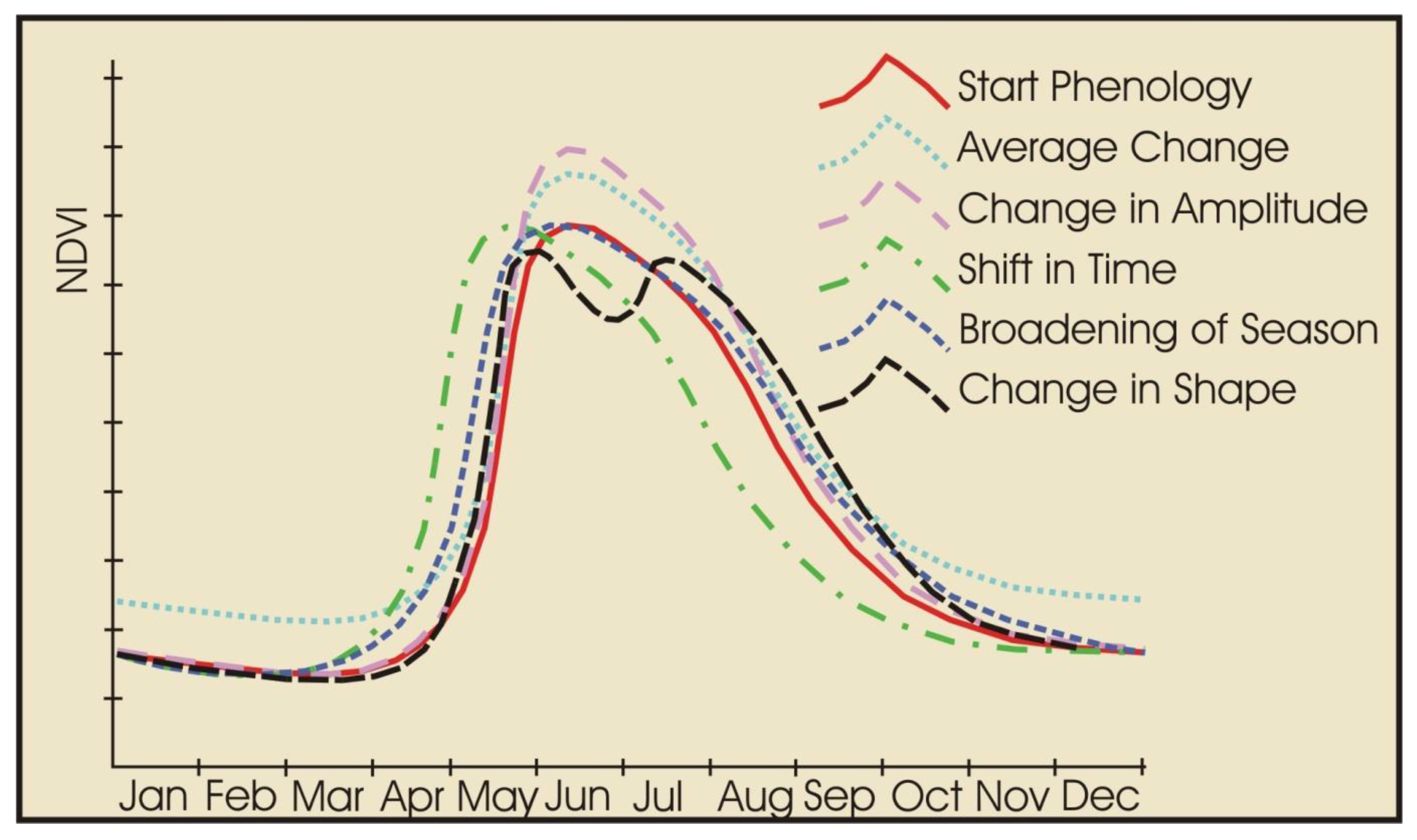
These considerations lead to the hypothesis that the integrated phenological curve as detected from remotely sensed image data can change in one or more of the five ways depicted in Figure 1. These five ways are:

• A change in the amplitude of the Phenological Curve. For example in areas that are moisture constrained, a trend of increasing rainfall in the growing season may result in an increase in peak greenness relative to the greenness out of the growing season.
• A change in average greenness throughout the year, by for example the replacement of evergreen needle leafed with evergreen broad leafed species.
• A shift in the time of the peak of the growing season as can occur when, for example, annual species are affected by changes in the temperature and/or rainfall regimes, leading to shifts in the phenophases associated with growth, maturation and death.
• A lengthening of the growing season yielding a broader or narrower phenological trajectory through time as can occur for example with rising or falling temperatures in areas that are temperature constrained.
• A change in the shape of the phenological curve, for example by the emergence of multiple peaks in the growing season caused by the invasion of species with different growth cycles, or due to changes in the rainfall regime.

Figure 1. The five ways that the phenological profiles as recorded in image data can change over time in comparison with the starting phenological curve (Start Phenology).

Figure 1. The five ways that the phenological profiles as recorded in image data can change over time in comparison with the starting phenological curve (Start Phenology).

Several authors have looked at alternative ways to describe the phenological profile from image data. Some workers have fitted generic functions to the phenology and then used these functions to retrieve metrics for subsequent analysis [34,35]. Others have used the Fourier transform [36,37] to retrieve metrics describing the phenology and then linked those metrics to climate data for their study areas in South and North America respectively. These studies have all placed constraints on the shape of the phenological curve, where these constraints may or may not be valid. This paper derives a suite of five integrated Phenological Change Indices that assume that the NDVI at a particular time in the season may change from season to season as a simple polynomial function but which makes no assumptions about how the shape of the phenological curve will change from season to season. These Phenological Change Indices (PCIs) are defined and described and some of the changes detected in the PCIs across Eurasia are discussed.

2. Data Sets Used in This Analysis

The GIMMS NDVI [38,39] data set from 1982 to 2008 has been used in this analysis. The source image data for this data set was collected using six different AVHRR sensors that acquired images over this time period. No correction has been applied to the source data for atmospheric effects due to water vapor, Rayleigh scattering or ozone. Maximum value compositing has been used, implemented with a forward binning procedure [38]. A stratospheric aerosol correction was applied from April 1982 to December 1984 and from June 1991 to December 1993, to correct for atmospheric aerosols due to volcanic eruptions [40]. This correction used a hybrid of retrieved optical thickness [41] and model estimates from atmospheric corrections software. Artefacts in the NDVI record due to satellite drift have been corrected using the empirical mode decomposition [42].

The resampled time series is at 8 km spatial resolution and twice per month temporal resolution, using the Albers Equal Area projection. The data are recorded as signed 16 bit integer data in the range −10,000 to 10,000 so that the data have to be divided by 10,000 to get NDVI values. The data set is partitioned into continental areas, of which the African and Eurasian continental datasets have been used in this study. The source time series was imported into Imagine, built into an image stack covering the relevant period of the time series (1982 to 2008) giving a total of 648 images in the stack. This stack was then exported as a generic binary file for derivation of the Phenological Change Indices.

Land cover data used in the study has been taken from the GlobCover land cover mapping (2005) [43] and the 1Km resolution Global Land Cover Mapping conducted by the University of Maryland [44] (UMD 1-km Land Cover Map). The GlobCover land cover mapping is based on 300-m spatial resolution MERIS data acquired in 2005. Processing of the data first developed mosaics of reflectance in 13 spectral bands, followed by an automated classification and expert labeling phase to produce a 22 class global land cover product on the Plate-Carree projection. Continental land cover maps have also been developed that contained sub-divisions of some of these classes as appropriate for the individual continents. A total of 18 land cover classes were sampled in this study across West Africa and used to define training areas to extract phenological profiles for the different cover types. These profiles were used for the work discussed in Section 4 of validating the indices by investigating how the indices changed with simulated changes in the profiles.

The UMD 1 km Land Cover Map [44] is based on AVHRR Pathfinder data for the period 1981–1994. Training data were used as the basis for supervised classification using a decision tree classifier. The derived 14 class land cover map is projected using the Goode’s Projection at 1 km spatial resolution. This land cover data was used to identify training areas for the work described in Section 5 to analyze the relationship between the Phenological Change Indices and location in Eurasia.

3. Derivation of the Indices

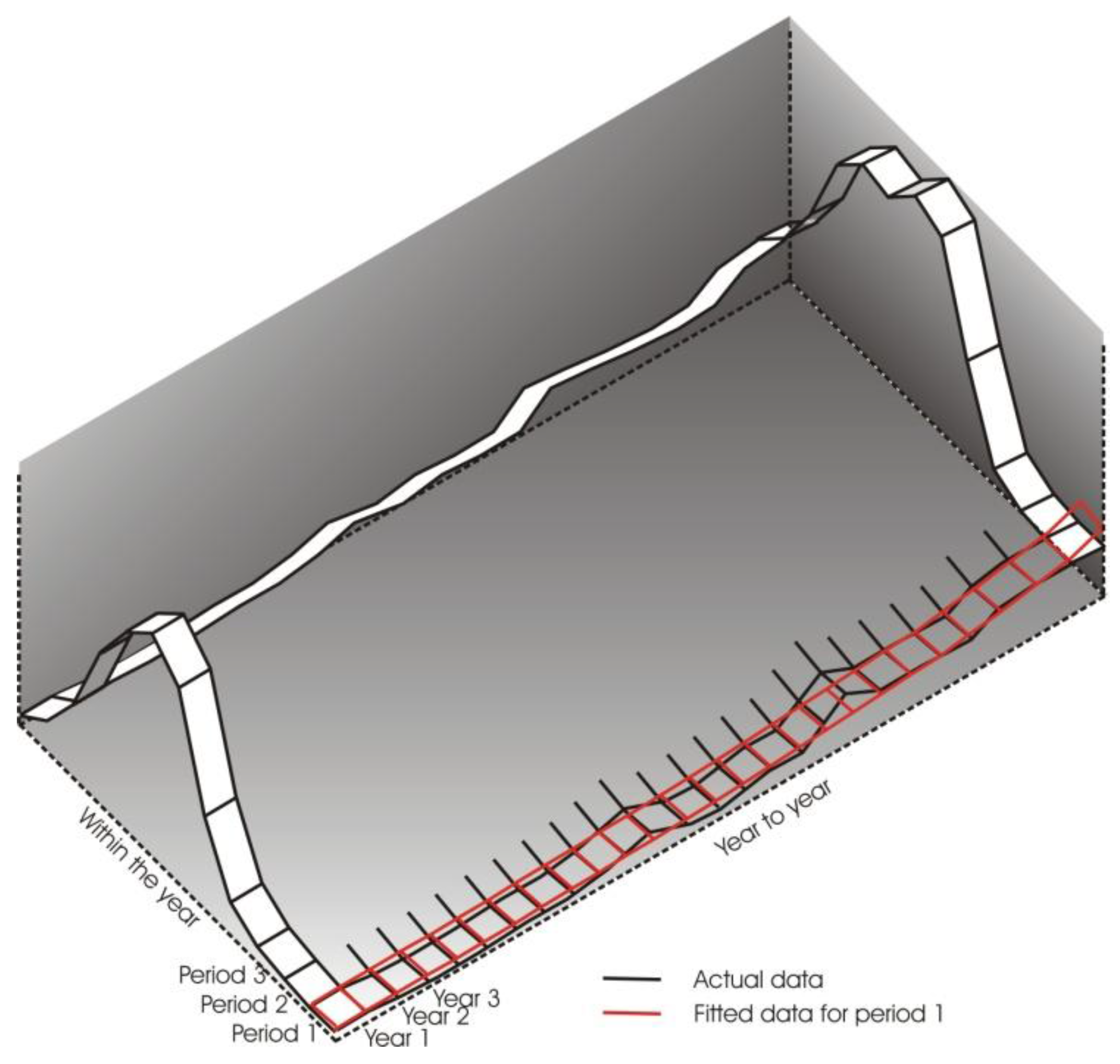
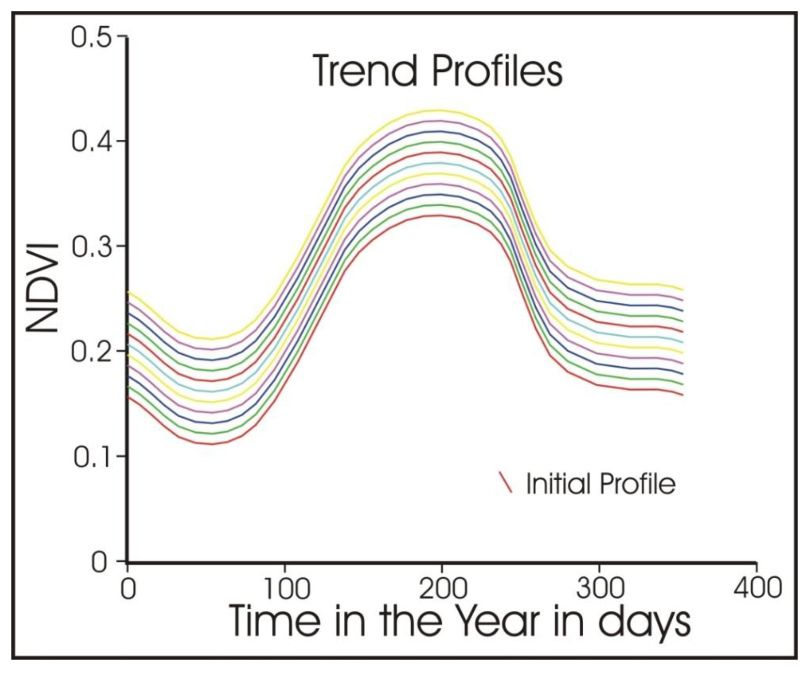
The development of the indices occurs in three stages for each pixel. The first stage (Fitting) derives a second order polynomial least squares fitting function for each within-year image date using the multi-year data from the time series for the fitting. This resulted in 24 fittings for the twice-per-month GIMMS time series (Figure 2). From each fitting values at the start and end of the period of analysis are derived. These are combined with similar values from each other fitting to build fitted phenological trajectories across the start and end years of the period of analysis. In the work reported here, the period of analysis is the same as the period of the time series, 1982–2008, but it could be a shorter period within this time range. This fitting is conducted to both reduce the effects of local weather on the NDVI profile and to reduce the effects of errors in the data.

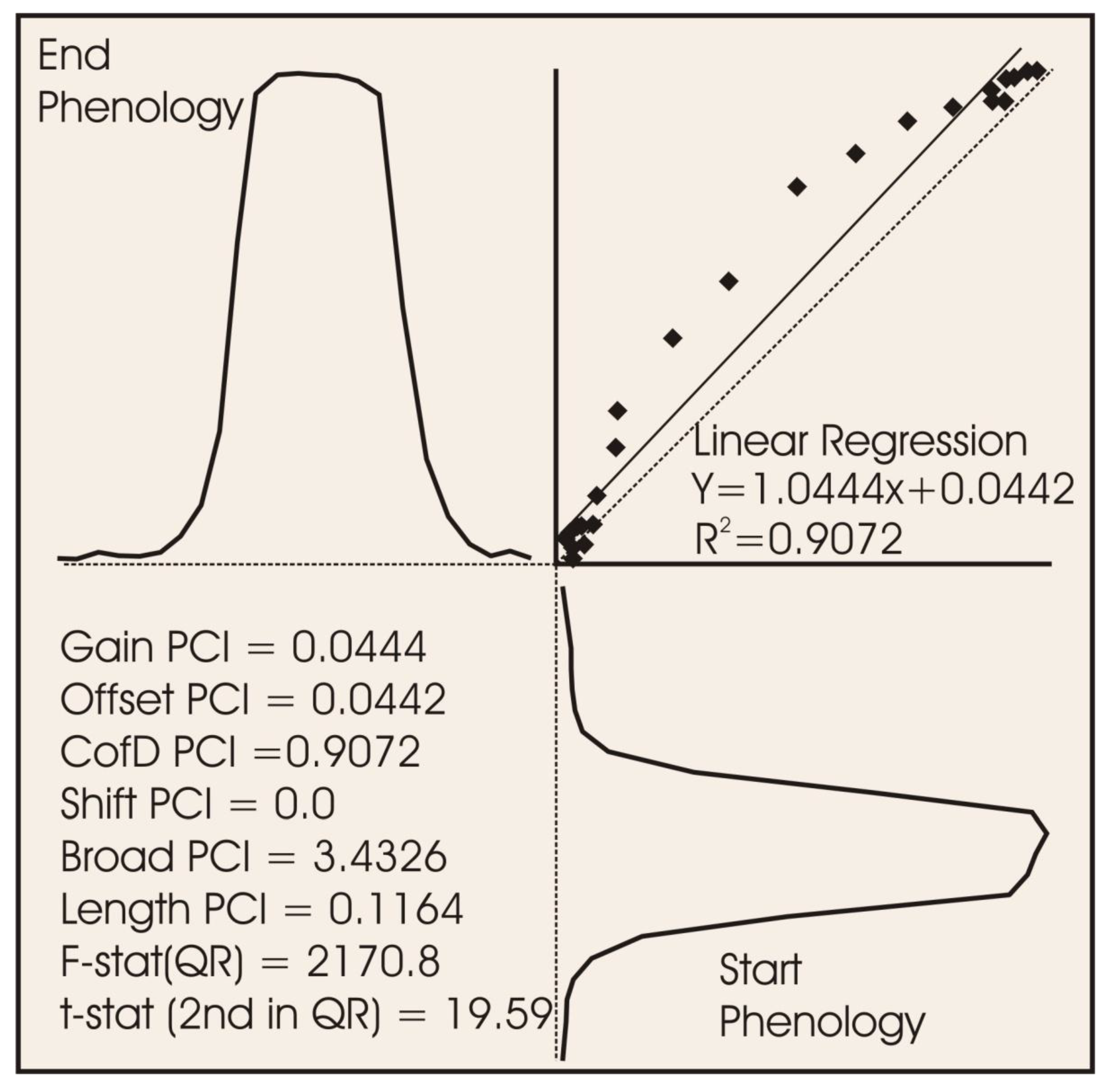
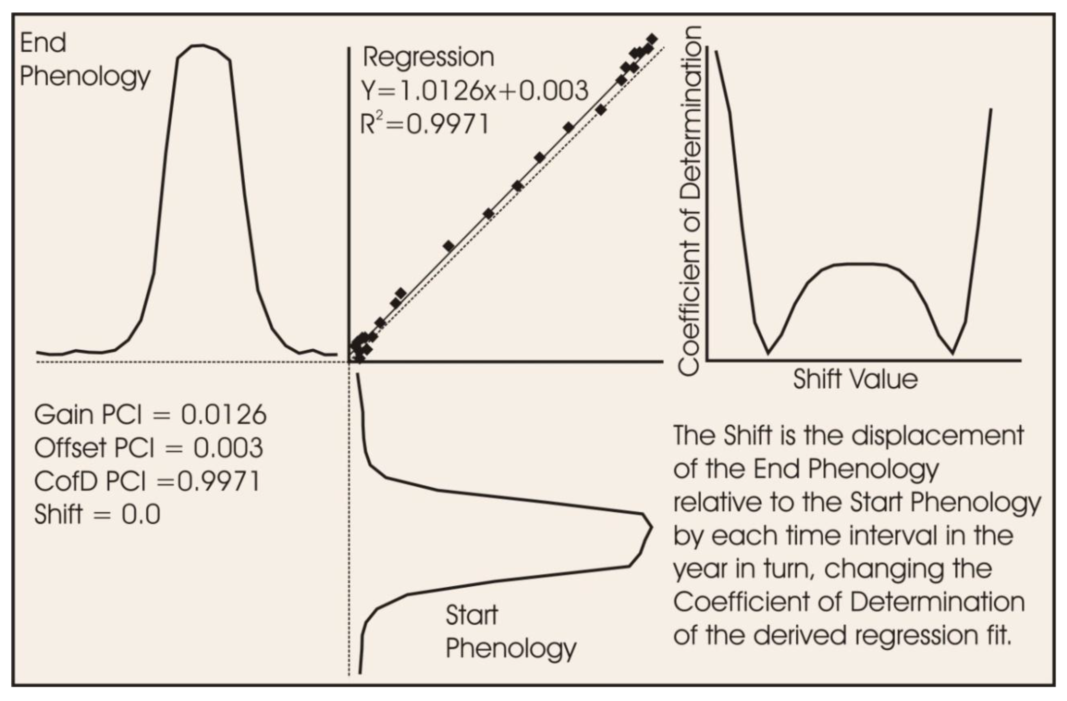
The second stage (Regression) is to conduct a series of linear regressions between the two fitted phenologies by shifting one phenology relative to the other by each of the possible time intervals in a year, in this case giving 24 regressions (Figure 3). The regression with the highest Coefficient of Determination is saved. The regression gives three Phenological Change Indices; the Gain Index, Offset Index and CofD Index and the shift between the phenological trajectories that yielded this Coefficient of Determination gives the fourth or Shift Index.

Figure 2. Least squares fitting of the data to a polynomial to smooth the data. The data across the years in each period of the annual cycle are fitted to a second order polynomial so as to smooth the data and thus minimize the effects of weather and errors in the data. Phenologies are taken from the fitted data at the start and end of the period of analysis; as is the case in this paper.

Figure 2. Least squares fitting of the data to a polynomial to smooth the data. The data across the years in each period of the annual cycle are fitted to a second order polynomial so as to smooth the data and thus minimize the effects of weather and errors in the data. Phenologies are taken from the fitted data at the start and end of the period of analysis; as is the case in this paper.

Sometimes higher Coefficients of Determination (R²) values can be achieved when the phenologies are completely out of phase. As a consequence the regression with the largest Regression Coefficient or R is selected.

The last stage (Residuals) is to derive an index that measures the lengthening or shortening of the growing season. A change in the length of the growing season has been found to be a common, but not the only, way by which a non-linear relationship between the data points in the regression can occur. If the season gets longer, then the residuals form a convex shape as shown in Figure 4, and conversely if the season shortens. Recognition of this led to the development of the Broad Index, defined as the difference between the weighted average of the data points falling within the central 50% and the weighted average of the data points falling in the outer two 25% percentiles, where the weights are inversely proportional to the data counts in each summation.

The Broad Index as developed does not include any test for statistical significance. As a consequence, an alternative index to measure the change in the length of the season has been developed, currently called the Length Index. This is derived by fitting a second order polynomial to the fitted phenologies, but only at the Shift that yielded the largest Coefficient of Determination in the simple linear regression. This second order polynomial regression is tested for significance using an F-test with a level of significance as set by the operator; here 5% has been used. If the F-test shows that the fit is not significant, then none of the PCIs are accepted and the pixel is mapped as having no significant phenology. If the F-test shows that the fitting is significant, then the significance of the second order term is tested using a t-test. The level of significance for this test is also set by the operator; here 10% has been used. If the t-test is not significant then the Length index is set to zero and the values of the other indices are derived using the linear regression. If the t-test is significant, then the Length Index is computed as the area between the second order polynomial and a line joining the end values in the second order function; the other indices are derived as before. Both the Broad and Length Index values are positive if the season gets longer, and are negative if it gets shorter.

Figure 3. Comparison of the phenologies derived from the fitted data by means of linear regression, and comparing the Start Phenology with the End Phenology starting at each time step in the phenology, selecting the regression with the largest Coefficient of Determination and saving the step as the Shift Index.

Figure 3. Comparison of the phenologies derived from the fitted data by means of linear regression, and comparing the Start Phenology with the End Phenology starting at each time step in the phenology, selecting the regression with the largest Coefficient of Determination and saving the step as the Shift Index.

Thus there are two Phenological Change Indices that measure the change in the length of the season; the Broad and Length Indices. The Broad Index is measured for all pixels for which the first four indices are measured and the Length Index is only measured if the t-test for the second order polynomial term is significant. This process thus provides a suite of six Phenological Change Indices (PCIs). Two of these indices (Broad and Length Indices) are meant to measure the change in the length of the season. One, the Shift Index is derived independently from the other indices and thus is unlikely to be correlated with the other indices. The indices are summarized as follows:

1

Gain Index; derived from the slope of the linear regression line with the largest Regression Coefficient. It primarily measures the change in the amplitude in the phenological profile. A Regression gain value of 1.0 means no change in the amplitude of the profile. A value of one has been subtracted from the regression gain value to obtain the Gain Index so that an index value of zero indicates no change; a positive value indicates an increase in amplitude and negative values indicate a decrease. It is dimensionless, being proportional to the amplitude of the initial phenological profile.

Figure 4. The relationship between the phenologies in the regression, when the end phenology has a symmetrically longer growing season than the start phenology. This leads to significant values in both the Broad and Length Indices. The displayed F statistic is for the Quadratic Function and the t statistic is for the second order term in that regression equation.

Figure 4. The relationship between the phenologies in the regression, when the end phenology has a symmetrically longer growing season than the start phenology. This leads to significant values in both the Broad and Length Indices. The displayed F statistic is for the Quadratic Function and the t statistic is for the second order term in that regression equation.

2

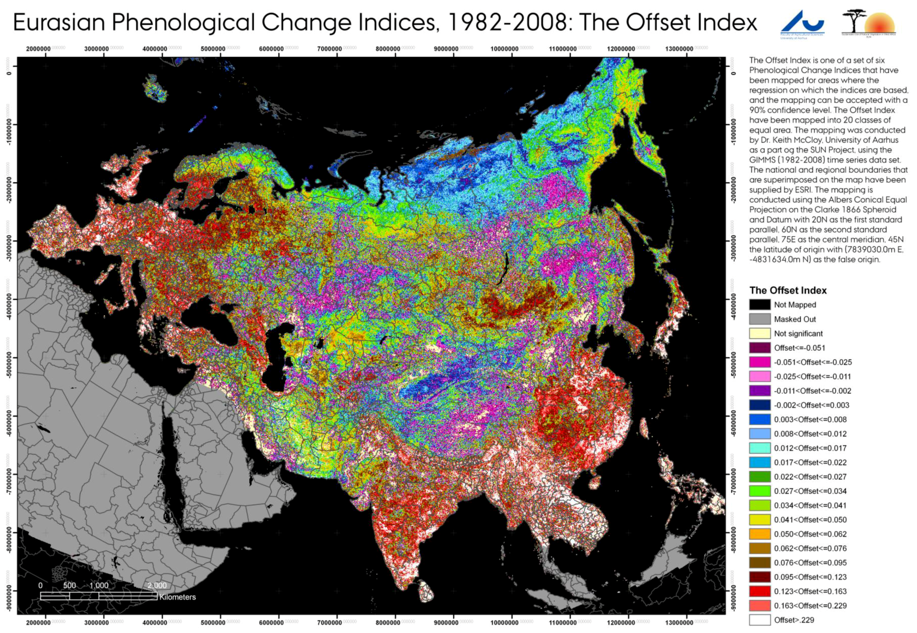
Offset Index; comes from the offset value from the same regression line and primarily measures the change in average annual greenness over the period of analysis. A value of zero indicates no change in the average annual value for NDVI, whilst positive values indicate an increase in the average value, and negative values a decrease. It is measured in the units of the data; NDVI in the case of the data used in this paper.

3

Shift Index; is the time shift between the fitted phenological profiles providing the linear regression with the largest Regression Coefficient. It has a value in days in this work, although it could just as easily be allotted other time dimensions, with the interval between values matching the interval between data values in the time series within one year. Negative values indicate that the peak of the end phenology is earlier than the peak of the start phenology, and vice versa.

4

CofD Index; Or the Coefficient of Determination of the linear regression with the largest Regression Coefficient. It provides information on the change in the shape of the phenological curve over the period of comparison and is dimensionless.

5

Broad or Length Indices; Both indices measure the deviation of the residuals from being randomly distributed around the regression line when the shape of the curve created by the residuals is similar to a second order polynomial. Such shapes occur when one phenological curve exhibits a change in the length of the growing season relative to the other phenological curve. Such a shape can also occur when the phenology changes shape to a bi-modal distribution. The Broad Index is easy to compute, but it has no sound statistical basis, nor is it easy to relate to the extension of the growing season. It is measured in units of the data. The Length Index is formed from the statistical analysis of the data and will only have values if the regression is statistically significant at the level set by the user. It is related to the extension of the season through the shape of the phenological curve. The Length Index is in units of area.

Software was built to develop Phenological Change Indices on a per-pixel basis from the Generic Binary image stacks derived from the source GIMMS time series datasets.

4. Testing the Derived Phenological Change Indices Using Simulating Data

Sample phenologies were used to build a number of simulated datasets. Each dataset contained twenty simulated phenologies as well as the original phenology, reflecting different values of the trend, t; change in peak amplitude, a; or the lengthening of the season, b; depending on the simulated dataset. Simulated datasets were not built to emulate changes in the shape of the phenological curve as measured using the CofD Index, or changes in the time of the peak as measured using the Shift Index.

4.1. Trend, t

A trend is used here as a change in the average annual NDVI value throughout the annual phenological trajectory over a period of years. If there is a trend of this type, then the end phenology at time i within the phenology (y_i) can be stated in relation to the start phenology (x_i) in the form:

$$y_i=x_i+t$$

(1)

in which t is the trend or the average change throughout the year between the start and the end phenological profiles. In such a situation, it can be shown that the linear regression between these two variables yields a regression equation with a gain value of 1.0 and an offset value of t.

4.2. Change in Peak Amplitude, a

The amplitude is defined as the difference in value between the trough and the peak values in a phenological trajectory. If there is a change in amplitude over the years of the time series, then the values in the end phenology, y_i are related to the values in the start phenology x_i of the form:

$$y_i=x_r+a\left(x_i-x_r\right)=a{x}_i+x_r\left(1-a\right)$$

(2)

in which x_r is the reference value in the start phenology about which the change in amplitude will take place and a is the change of the amplitude. A value of a = 1.0 means that there is no change in amplitude between the start and the end phenological trajectories. The linear regression between these two sets of data will yield a gain value of a and an offset value of $x_r\left(1-a\right)$. If the reference value, x_r is close to zero, as is the case with NDVI data, then the linear regression gives a gain value that is the same as the change in amplitude of the data and an offset that is small and of opposite sign to this change.

4.3. Lengthening of the Growing Season, b

Should the season become longer over the years of the time series, the relationship between the phenological trajectories takes the form:

$$y_i=x_i+b\left(x_i-x_{min}\right)\ast \left(x_{max}-x_i\right)$$

(3)

where x_min and x_max are the minimum and maximum values in the start phenology and b is the amount by which the value x_i will be changed to yield the y_i values at the end phenological trajectory, then the linear regression gain and offset values are:

$$Gain=\alpha =\frac{n{{\displaystyle \sum }}^{\text{}}xy-{{\displaystyle \sum }}^{\text{}}x\ast {{\displaystyle \sum }}^{\text{}}y}{Den}=1+b\left(x_{max}+x_{min}\right)-\frac{nb{{\displaystyle \sum }}^{\text{}}{x}^3-b{{\displaystyle \sum }}^{\text{}}x{{\displaystyle \sum }}^{\text{}}{x}^2}{Den}$$

(4)

$$Offset=\beta =\frac{{{\displaystyle \sum }}^{\text{}}y{{\displaystyle \sum }}^{\text{}}{x}^2-{{\displaystyle \sum }}^{\text{}}x\ast {{\displaystyle \sum }}^{\text{}}xy}{Den}=-b\left(x_{max}*x_{min}\right)-\frac{b{{\displaystyle \sum }}^{\text{}}x{{\displaystyle \sum }}^{\text{}}{x}^3-b{{\displaystyle \sum }}^{\text{}}{x}^2{{\displaystyle \sum }}^{\text{}}{x}^2}{Den}$$

(5)

where $Den=n{{\displaystyle \sum }}^{\text{}}{x}^2-{{\displaystyle \sum }}^{\text{}}x{{\displaystyle \sum }}^{\text{}}x$. It can be seen that a lengthening of the season of this form introduces a linear component into both the Gain $\left(1+b\left(x_{min}+x_{max}\right)\right)$ and Offset $\left(-b{x}_{min}{x}_{max}\right)$ terms that are a function of the maximum and minimum values in x and b and a non-linear component that is a function of various sums of product terms.

The simulations were based on samples taken from the GIMMS time series dataset [38], for the 18 land covers sampled in West Africa from the GlobCover2005 land cover mapping [43]. Sample 2005 phenological trajectories were derived for each land cover class, ensuring that the samples were as large as possible. Some land covers only occurred in small areas, such as the urban and the water classes, so that their sample sizes were small, but most were in larger contiguous areas and so their sample sizes varied from 167 to 1,932 pixels. Mean 2005 phenological trajectories for these sample areas were derived using Imagine image processing software and these were exported to spreadsheet software for subsequent analysis.

Each 2005 phenological trajectory was then modified using Equations (1–3) and with twenty different values in t, a and b respectively, to give three sets of 21 different phenological trajectories, representing the start trajectory and the 20 changed trajectories. The three sets of trajectories for different values in t, a and b for the one land cover sample are shown in Figure 5, Figure 6 and Figure 7.

Each of the 20 phenological trajectories in a set was then compared with the start trajectory so as to derive twenty sets of six Phenological Change Indices (Gain, Offset, Shift, CofD, Broad and Length). These PCIs were then plotted against the value of t, a or b used to create the phenological trajectory as shown in Figure 8, Figure 9 and Figure 10 for the same land cover. The Length Index gave similar results to that of the Broad Index, and so it has not been shown in these figures.

Figure 5. The set of 21 simulated phenological profiles created using different trend values (t) in the range 0.005–0.1 for GlobCover Class 11. The initial profile is the lowest red profile.

Figure 5. The set of 21 simulated phenological profiles created using different trend values (t) in the range 0.005–0.1 for GlobCover Class 11. The initial profile is the lowest red profile.

Figure 6. The set of 21 simulated phenological profiles created using different amplitude values (a) in the range 0.015–0.3 for GlobCover Class 11. The initial profile is the lowest red profile.

Figure 6. The set of 21 simulated phenological profiles created using different amplitude values (a) in the range 0.015–0.3 for GlobCover Class 11. The initial profile is the lowest red profile.

Figure 7. The set of 21 simulated phenological profiles created using different broadening values (b) in the range 0.03–0.6 for GlobCover Class 11. The initial profile is the lowest red profile.

Figure 7. The set of 21 simulated phenological profiles created using different broadening values (b) in the range 0.03–0.6 for GlobCover Class 11. The initial profile is the lowest red profile.

Figure 8. Changes in the Phenological Change Indices, with changes in the trend parameter, t, using the set of 21 phenological profiles in Figure 5. There are 20 values along each of the lines plotted in the figure because each of the 20 profiles is compared to the source profile in the derivation of the PCI values for that profile.

Figure 8. Changes in the Phenological Change Indices, with changes in the trend parameter, t, using the set of 21 phenological profiles in Figure 5. There are 20 values along each of the lines plotted in the figure because each of the 20 profiles is compared to the source profile in the derivation of the PCI values for that profile.

Figure 9. Changes in the Phenological Change Indices, with changes in the amplitude parameter, a, using the set of 21 phenological profiles in Figure 6. There are 20 values along each of the lines plotted in the figure because each of the 20 profiles is compared to the source profile in the derivation of the PCI values for that profile.

Figure 9. Changes in the Phenological Change Indices, with changes in the amplitude parameter, a, using the set of 21 phenological profiles in Figure 6. There are 20 values along each of the lines plotted in the figure because each of the 20 profiles is compared to the source profile in the derivation of the PCI values for that profile.

Figure 10. Changes in the Phenological Change Indices, with changes in the broadening parameter, b, using the set of 21 phenological profiles in Figure 7. There are 20 values along each of the lines plotted in the figure because each of the 20 profiles is compared to the source profile in the derivation of the PCI values for that profile.

Figure 10. Changes in the Phenological Change Indices, with changes in the broadening parameter, b, using the set of 21 phenological profiles in Figure 7. There are 20 values along each of the lines plotted in the figure because each of the 20 profiles is compared to the source profile in the derivation of the PCI values for that profile.

4.4. Results of this Analysis

Figure 8 shows that, as predicted, a trend in the data will yield linear changes in the Offset Index, but that it has no effect on the other Phenological Change Indices. Figure 9 shows that a change in the amplitude of the phenological profile introduces the predicted linear change in the Gain Index of the same magnitude as the change in amplitude, and a smaller linear change in the Offset Index of opposite sign to that of the Gain Index; with no effect on the other indices. Figure 10 shows that a change in the length of the season affects all of the Phenological Change Indices. For smaller increases in the length of the season, the Broad and Length Indices increase in proportion to the lengthening of the season, but as the season becomes even longer, so the increases in these indices start to decline until the indices do not change for very large increases in the length of the season. For small increases in the season length, the effect on the Offset Index is negligible, but as the season gets longer progressively larger increases in the Offset Index are observed. The CofD Index steadily declines with increasing length of the season, and the Gain Index initially increases and then declines. The way that these indices change with a longer season, depends very much on the shape of the phenological profile. In some cases, the CofD Index is closely related to a broadening of the season, as occurs in Figure 10, but this is not always the case. Further, the CofD Index changes with changes in shape, so that complex changes in the phenological profile will induce changes in the CofD Index, whereas they should not in the Broad or Length Indices.

These simulations show that, in general, the largest impact of a change in the phenological profile is on the index meant to measure that type of change; the impact on the other indices is small. However, this work also shows that care needs to be taken in the interpretation of the indices as some of the changes in one or more of the indices will be in part due to artifacts resulting from the effects of changes in the other indices. In other cases the impacts of different processes may cancel them out.

5. Analysis of the Relationship between the Phenological Change Indices and location in Eurasia

Phenological Change Indices were derived between 1982 and 2008 using the GIMMS time series dataset (1982–2008) [38] for Eurasia as depicted in the following figures, where the indices were only mapped for areas where the F-test of the regression met the 90% Confidence Limit. These PCIs were analyzed in relation to position (Latitude, Longitude) and land cover type using the University of Maryland 1 Km resolution Global Land cover map of 1998 [44].

The land cover map was re-projected to match the Albers Equal Area projection and resolution of the GIMMS time series data by using a rigorous re-projection algorithm with nearest neighbor resampling. A total of 172 training areas or samples were selected by:

• Visually identifying contiguous areas that appeared to contain only the one cover type on at least 90% of the pixels within the sample.
• Adjusting the sample boundary until this criterion was met through pixel counting in the samples.
• That each sample contained at least 30 pixels. This criterion could not always be met because some covers occurred in small dis-aggregated areas. As a consequence, the smallest sample contained 14 pixels, the largest 1602 pixels and the average sample size was 194.5 pixels.
• Find as many samples as possible that met these criteria, the number selected being listed in Table 1.

Table 1. The land cover codes, cover types, number of samples used in this study, the range of latitudes covered by these samples and the acronym used in the figures.

Code	Cover Type	Cover Min Latitude(°N)	Cover Max Latitude(°N)	Sample Count	Acronym
0	Ocean	None	None	0	Ocean
1	Evergreen needleleaf forest	50	60	15	ENFor
2	Evergreen broadleaf forest	12	26	5	EBFor
3	Deciduous needleleaf forest	54	63	4	DNFor
4	Deciduous broadleaf forest	43	60	4	DBFor
5	Mixed forest	47	60	14	MxFor
6	Woodland	15	64	10	WdLnd
7	Wooded grassland	18	69	17	WGLnd
8	Closed shrubland	37	70	10	CSLnd
9A	Open shrubland, Latitude < 60°N	25	56	21	OSLnd(A)
9B	Open shrubland, Latitude > 60°N	63	75	27	OSLnd(B)
10	Grassland	12	55	20	GrLnd
11	Cropland	30	55	18	CrLnd
12	Bare Ground	40	48	7	Bare
13	Urban and Builtup	None	None	0	Urban

Table 1. The land cover codes, cover types, number of samples used in this study, the range of latitudes covered by these samples and the acronym used in the figures.

Code	Cover Type	Cover Min Latitude(°N)	Cover Max Latitude(°N)	Sample Count	Acronym
0	Ocean	None	None	0	Ocean
1	Evergreen needleleaf forest	50	60	15	ENFor
2	Evergreen broadleaf forest	12	26	5	EBFor
3	Deciduous needleleaf forest	54	63	4	DNFor
4	Deciduous broadleaf forest	43	60	4	DBFor
5	Mixed forest	47	60	14	MxFor
6	Woodland	15	64	10	WdLnd
7	Wooded grassland	18	69	17	WGLnd
8	Closed shrubland	37	70	10	CSLnd
9A	Open shrubland, Latitude < 60°N	25	56	21	OSLnd(A)
9B	Open shrubland, Latitude > 60°N	63	75	27	OSLnd(B)
10	Grassland	12	55	20	GrLnd
11	Cropland	30	55	18	CrLnd
12	Bare Ground	40	48	7	Bare
13	Urban and Builtup	None	None	0	Urban

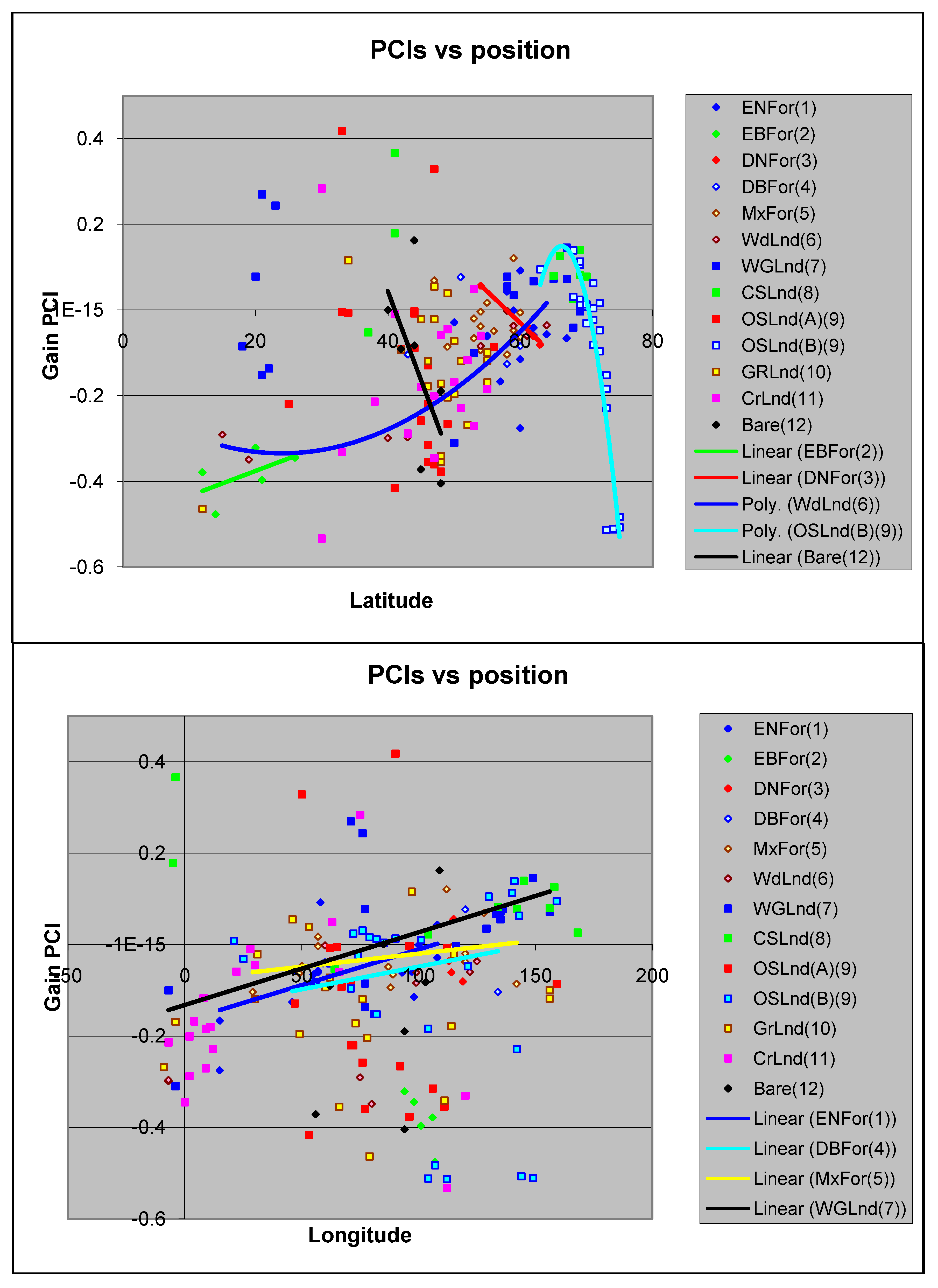
An important question in climate change research is whether phenological trends are related to geographic location. To test this, the sample mean values for all six PCIs were derived for the 172 training areas and then plotted against both the centroid latitude and longitude for the training areas. Both latitude and longitude were chosen because significant north-south trends and east-west zonation in some latitude zones was found in changes in early season phenophases by [33]. Figure 11 shows this plot for the Gain Index and Figure 12 for the Broad Index. Regressions were conducted for classes 1 to 12 inclusive using first latitude and then longitude as the independent variable and the Index as the dependent variable. Some of these regressions are shown in Figure 11 and Figure 12, noting that both latitude and longitude are positive in Eurasia. In all cases the Open Shrubland class (Class 9) showed quite different characteristics at latitudes higher than 60°N than at lower latitudes and so the analysis of this class has been conducted in these two sub-classes.

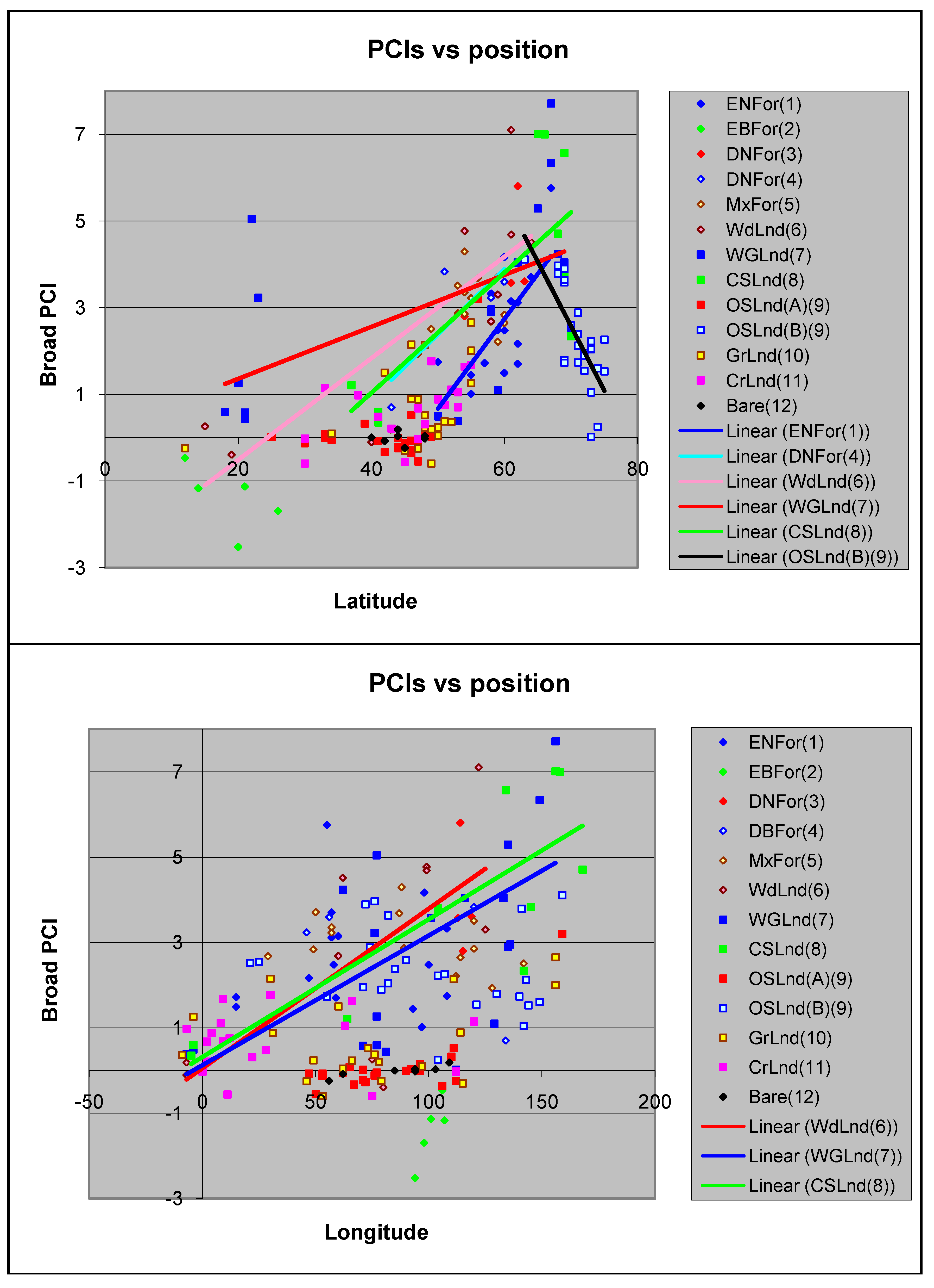
The results of the analysis of the Gain and Broad PCIs are shown in Figure 11 and Figure 12 in relation to latitude and longitude respectively, and the main results are summarized in Table 2 and Table 3. Whilst there are general trends of some PCIs across the different land covers, in fact the dominant finding is that the different land covers respond in quite individual ways to climate change, as seen in Table 2 and Table 3.

Figure 11. Gain PCI vs. latitude and longitude and some of the trends as a function of latitude and longitude.

Figure 11. Gain PCI vs. latitude and longitude and some of the trends as a function of latitude and longitude.

Figure 12. Broad PCI vs. latitude and longitude and some of the trends detected as a function of latitude and longitude.

Figure 12. Broad PCI vs. latitude and longitude and some of the trends detected as a function of latitude and longitude.

Ten of the 13 classes exhibited an increase in the length of the season. Of these ten, three exhibited a positive change with latitude, four with both latitude and longitude and one class exhibited a negative change from large increases to smaller increases in the length of the season, and the remaining two classes exhibited an increase in the length of the season at all latitudes. In all cases the change was to longer seasons.

Six of the 13 classes exhibited a reduction in amplitude with higher latitude and a further four exhibited changes in amplitude with longitude. Of the six classes that exhibited changes with latitude, three exhibited positive changes with increasing latitude, two negative changes with increasing latitude, and one the same change at all latitudes. All four classes that exhibited a change with longitude showed a positive change, with one class having reductions in amplitude, one no average change, and two showing an increase in amplitude.

Five of the 13 classes exhibited an increase in average greenness with increasing latitude and one class exhibited a negative change of decreasing greenness with increasing longitude.

Table 2. Summary of changes in phenological attributes, as measured by Phenological Change Indices as a function of latitude, for the major land covers.

Land Cover Class	Dominant changes detected in this analysis as a function of latitude
Evergreen needleleaf forest	Positive linear trend between latitude and longer seasons
Evergreen broadleaf forest	Positive linear trend between latitude and amplitude, from large reductions in amplitude to smaller reductions. Large increases in average annual greenness at all latitudes and shift to earlier peak greenness.
Deciduous needleleaf forest	Longer seasons at all latitudes
Deciduous broadleaf forest	Positive linear trend between latitude longer seasons
Mixed forest	Longer seasons at all latitudes
Woodland	Positive non-linear trend between latitude and amplitude from large reductions in amplitude to no change in amplitude. Increase in annual average greenness at all latitudes and a positive linear trend between latitude and longer seasons.
Wooded grassland	Positive linear trend between latitude and longer seasons
Closed shrubland	Positive linear trend between latitude and longer seasons
Open shrubland, Latitude < 60°N	Neither trends nor changes detected in the PCIs.
Open shrubland, Latitude > 60°N	Negative non-linear trend between latitude and amplitude from increases to decreases in amplitude. Negative linear trend between latitude and longer seasons from much longer to marginally longer seasons.
Grassland	Decrease in the amplitude of the peak; increase in average annual greenness; positive non-linear trend between latitude and longer seasons.
Cropland	Positive linear trend between latitude and amplitude from large decreases in amplitude to small increases; increase in annual average greenness; positive linear trend between latitude and longer seasons.
Bare Ground	Negative linear trend between latitude and amplitude; increase in annual average greenness.

Table 2. Summary of changes in phenological attributes, as measured by Phenological Change Indices as a function of latitude, for the major land covers.

Land Cover Class	Dominant changes detected in this analysis as a function of latitude
Evergreen needleleaf forest	Positive linear trend between latitude and longer seasons
Evergreen broadleaf forest	Positive linear trend between latitude and amplitude, from large reductions in amplitude to smaller reductions. Large increases in average annual greenness at all latitudes and shift to earlier peak greenness.
Deciduous needleleaf forest	Longer seasons at all latitudes
Deciduous broadleaf forest	Positive linear trend between latitude longer seasons
Mixed forest	Longer seasons at all latitudes
Woodland	Positive non-linear trend between latitude and amplitude from large reductions in amplitude to no change in amplitude. Increase in annual average greenness at all latitudes and a positive linear trend between latitude and longer seasons.
Wooded grassland	Positive linear trend between latitude and longer seasons
Closed shrubland	Positive linear trend between latitude and longer seasons
Open shrubland, Latitude < 60°N	Neither trends nor changes detected in the PCIs.
Open shrubland, Latitude > 60°N	Negative non-linear trend between latitude and amplitude from increases to decreases in amplitude. Negative linear trend between latitude and longer seasons from much longer to marginally longer seasons.
Grassland	Decrease in the amplitude of the peak; increase in average annual greenness; positive non-linear trend between latitude and longer seasons.
Cropland	Positive linear trend between latitude and amplitude from large decreases in amplitude to small increases; increase in annual average greenness; positive linear trend between latitude and longer seasons.
Bare Ground	Negative linear trend between latitude and amplitude; increase in annual average greenness.

Table 3. Changes in phenological attributes as measured by Phenological Change Indices and how these changes are a function of longitude.

Land Cover Class	Dominant changes detected in this analysis as a function of longitude
Evergreen needleleaf forest	Positive linear trend between longitude and amplitude from large reductions in amplitude in the west to small increases in the east; longer seasons at all longitudes.
Evergreen broadleaf forest	Large reduction in the Coefficient of Determination at mid longitudes.
Deciduous needleleaf forest	No significant changes or trends detected
Deciduous broadleaf forest	Positive linear trend between longitude and amplitude from small reductions in the west to small increases in the east.
Mixed forest	Positive linear trend between longitude and amplitude from no change in the west to small increases in the east.
Woodland	Positive linear trend between longitude and longer seasons.
Wooded grassland	Positive linear trend between longitude and amplitude; negative linear trend between longitude and average annual greenness; positive linear trend between longitude and longer seasons.
Closed shrubland	Positive linear trend between longitude and longer seasons.
Open shrubland, Latitude < 60oN	Large reduction in the Coefficient of Determination at mid longitudes
Open shrubland, Latitude > 60oN	Large reduction in the Coefficient of Determination at mid longitudes
Grassland	Large reduction in the Coefficient of Determination at mid longitudes, Negative linear trend between longitude and Shift to an earlier time of peak greenness.
Cropland	Large reduction in the Coefficient of Determination at mid longitudes
Bare Ground	Large reduction in the Coefficient of Determination at mid longitudes.

Table 3. Changes in phenological attributes as measured by Phenological Change Indices and how these changes are a function of longitude.

Land Cover Class	Dominant changes detected in this analysis as a function of longitude
Evergreen needleleaf forest	Positive linear trend between longitude and amplitude from large reductions in amplitude in the west to small increases in the east; longer seasons at all longitudes.
Evergreen broadleaf forest	Large reduction in the Coefficient of Determination at mid longitudes.
Deciduous needleleaf forest	No significant changes or trends detected
Deciduous broadleaf forest	Positive linear trend between longitude and amplitude from small reductions in the west to small increases in the east.
Mixed forest	Positive linear trend between longitude and amplitude from no change in the west to small increases in the east.
Woodland	Positive linear trend between longitude and longer seasons.
Wooded grassland	Positive linear trend between longitude and amplitude; negative linear trend between longitude and average annual greenness; positive linear trend between longitude and longer seasons.
Closed shrubland	Positive linear trend between longitude and longer seasons.
Open shrubland, Latitude < 60oN	Large reduction in the Coefficient of Determination at mid longitudes
Open shrubland, Latitude > 60oN	Large reduction in the Coefficient of Determination at mid longitudes
Grassland	Large reduction in the Coefficient of Determination at mid longitudes, Negative linear trend between longitude and Shift to an earlier time of peak greenness.
Cropland	Large reduction in the Coefficient of Determination at mid longitudes
Bare Ground	Large reduction in the Coefficient of Determination at mid longitudes.

The shift index is a coarse tool when used with the GIMMS data, because the twice monthly interval between the images in the time series does not record shifts of less than about 15 days. Despite this, seven of the classes showed a shift in the timing of peak growth, with five of these being to earlier and two to later peaks of growth. None of them showed correlation between the shift and latitude, but two classes showed correlation between the shift and longitude; in both cases having a shift to earlier peaks in the west and no shift in the east.

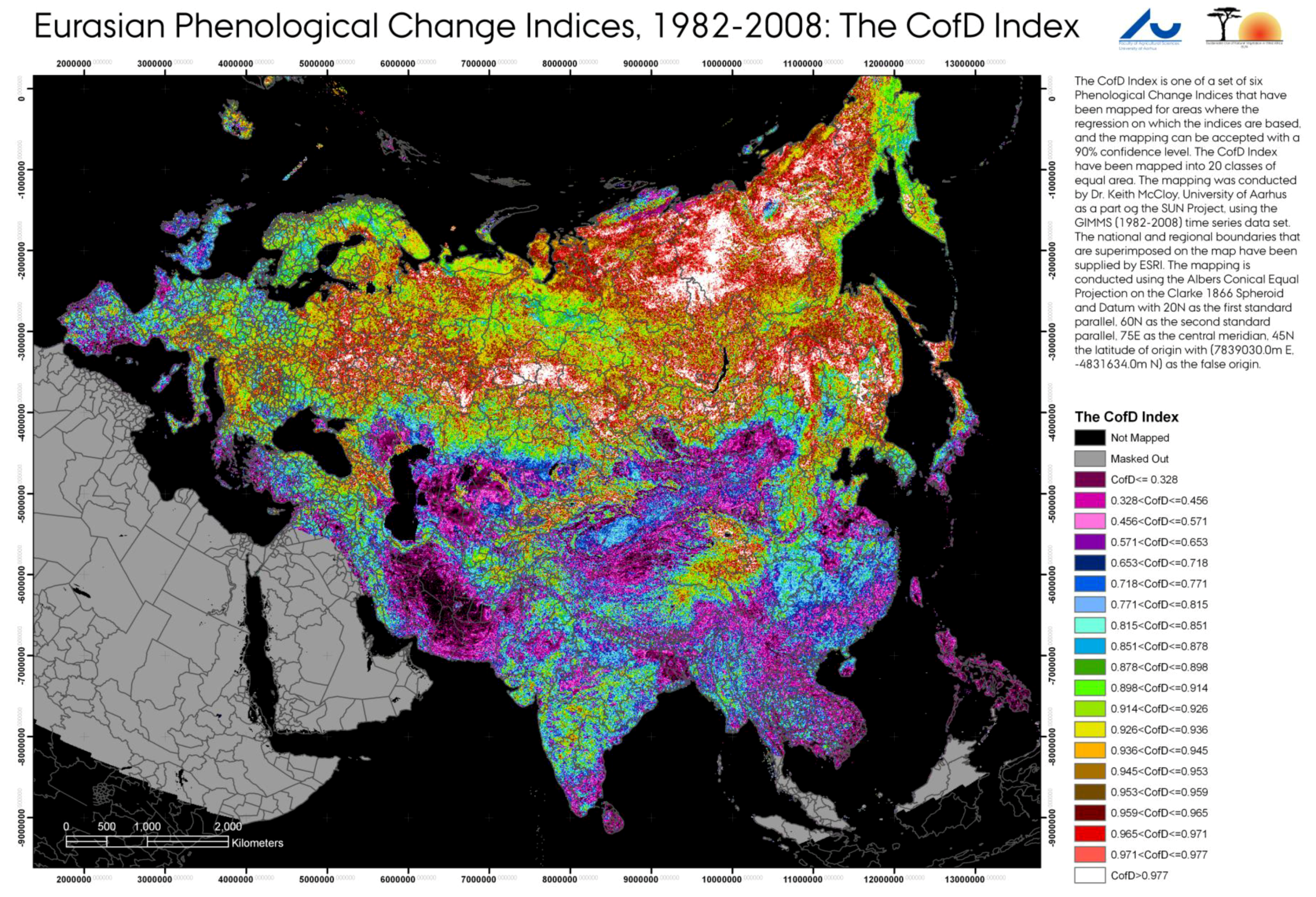
The Coefficient of Determination Index generally maintained high values at high latitudes both in the west and the east, but showed areas of significant change in the shape of the phenological curve at lower latitudes and at central (50–120°E) longitudes. That the changes in shape are concentrated at lower latitudes, suggests that many of these changes may be due in part to human activities.

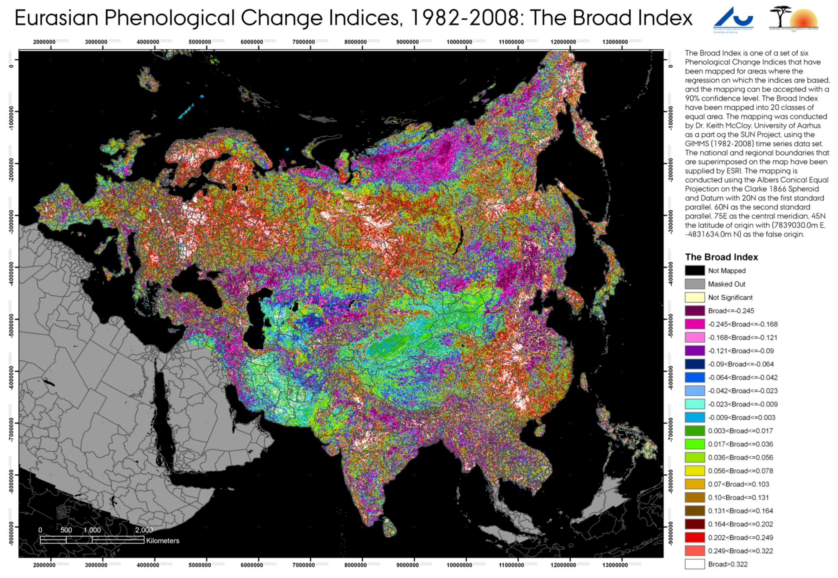
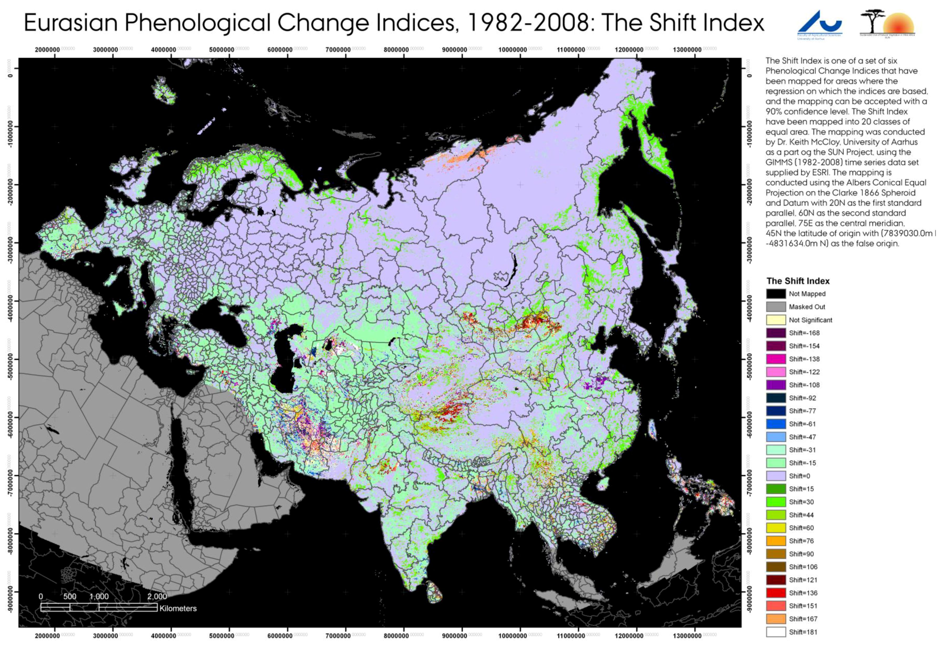
Perusal of the images of the six Phenological Change Indices (Figure 13, Figure 14, Figure 15, Figure 16, Figure 17 and Figure 18) shows small areas where the regression was not statistically significant at the 90% Confidence Level; shown as beige in color. The Broad Index shows large increases in the length of the season in central and northern Siberia, with the largest increases being at the higher latitudes, reinforcing conclusions reached in the analysis of the samples. There are large areas of shorter seasons including parts of Europe, much of coastal China, most of monsoonal South and South-East Asia and areas peripheral to deserts.

The Length Index is similar to the Broad Index, but it contains a much larger proportion of beige color, representing areas that were not statistically significant at the 90% Confidence Level for the second order term in the polynomial regression.

The Shift Index, that records changes in the timing of peak greenness, generally shows little change at high latitudes, with the exception of isolated areas of earlier peak greenness in the Scandinavian Peninsular, and an area of significantly later peak greenness in the extreme north of central Siberia near the Taymyr Peninsular. This area also has low CofD (curve shape change) values, suggesting that changes in land cover are taking place in this area. South of about 50°N, extensive areas of earlier peak greenness occur across Europe and the Middle East as far north as the elevated plateau of the Kirghiz Steppe and south into western India. Distinct areas show changes in the time of peak greenness; eastern India shows earlier peaks, China shows later peaks, and South East Asia shows no change.

The CofD Index (change in the shape of the phenological curve over time) shows negligible to small reductions in the CofD value and thus negligible to small changes in the shape of the phenological curve across most of Russia, with the exception of the Taymyr Peninsular as previously noted. South and west of Russia the CofD Index often declines significantly, particularly across South-East Asia, southern China, Bangladesh and parts of Europe. Many of these areas are subject to human pressure, and so man-induced land cover change is likely to be a major factor in the changes in shape of the phenological curve.

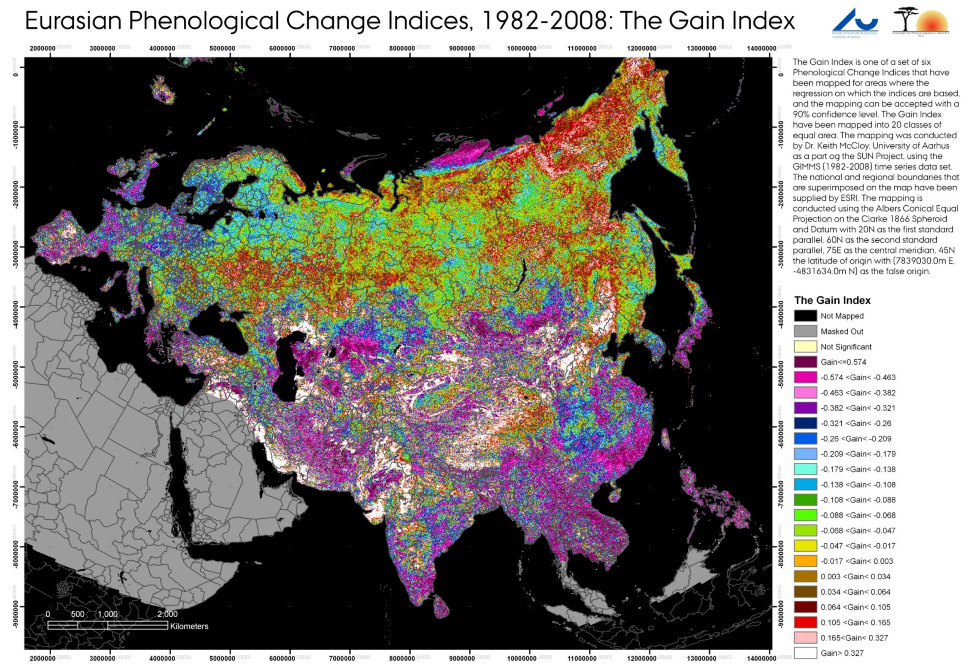
The Gain (amplitude change) and Offset (average change in greenness) Indices often act in concert, with reductions in one being matched by increases in the other, and vice versa. Thus much of Europe (excluding Russia outside of an area in the vicinity of the Baltic Sea), western Turkey, parts of The Caucasus, most of India, South-East Asia, eastern China and southern Japan, are all experiencing a decrease in the amplitude of peak growth and an increase in the average annual NDVI. In some parts of Europe this is happening because a portion of the croplands is being converted into either pasture or back into natural areas, with the attendant increase in out of season NDVI and consequent reduction in the amplitude of the peak. By contrast, most of Russia and parts of western China are experiencing an increase in amplitude and a reduction in average annual NDVI. Many areas that are peripheral to the deserts of Asia are experiencing an increase in amplitude and a decrease in average annual NDVI.

The picture is in fact very complex. In addition to the broader global climatic influences, there are clearly local forcing mechanisms being detected that are influencing the changes in plant phenology. In many cases these local influences, including elevation, micro-climatic mechanisms and human activities, dominate or strongly influence the detected trends. Only in the north of Eurasia are the effects of the global climate process clearly the dominant cause of the changes in phenology.

Figure 13. The Broad PCI, measuring the lengthening of the season. Derived using the GIMMS time series 1982–2008 [38].

Figure 13. The Broad PCI, measuring the lengthening of the season. Derived using the GIMMS time series 1982–2008 [38].

Figure 14. The Length PCI, measuring the change in the length of the season. Derived using the GIMMS time series 1982–2008 [38].

Figure 14. The Length PCI, measuring the change in the length of the season. Derived using the GIMMS time series 1982–2008 [38].

Figure 15. The CofD PCI, measuring the change in shape of the phenological profile. Derived using the GIMMS time series 1982–2008 [38].

Figure 15. The CofD PCI, measuring the change in shape of the phenological profile. Derived using the GIMMS time series 1982–2008 [38].

Figure 16. The Shift PCI, measuring the shift in the time of the peak of the season. Derived using the GIMMS time series 1982–2008 [38].

Figure 16. The Shift PCI, measuring the shift in the time of the peak of the season. Derived using the GIMMS time series 1982–2008 [38].

Figure 17. The Gain PCI, measuring the change in amplitude of the peak of the season. Derived using the GIMMS time series 1982–2008 [38].

Figure 17. The Gain PCI, measuring the change in amplitude of the peak of the season. Derived using the GIMMS time series 1982–2008 [38].

Figure 18. The Offset PCI, measuring the change in the average value throughout the season. Derived using the GIMMS time series 1982–2008 [38].

Figure 18. The Offset PCI, measuring the change in the average value throughout the season. Derived using the GIMMS time series 1982–2008 [38].

6. Discussion

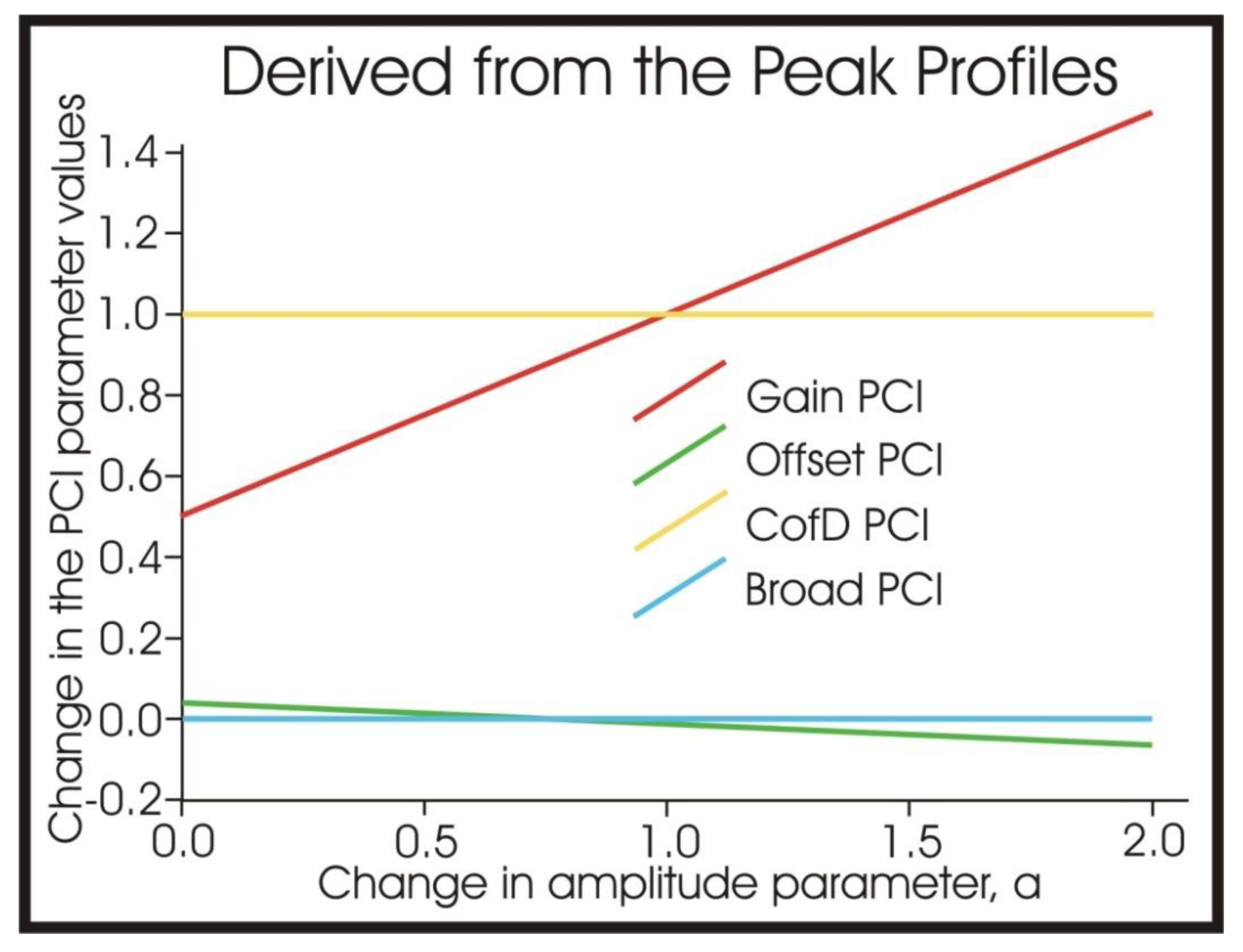
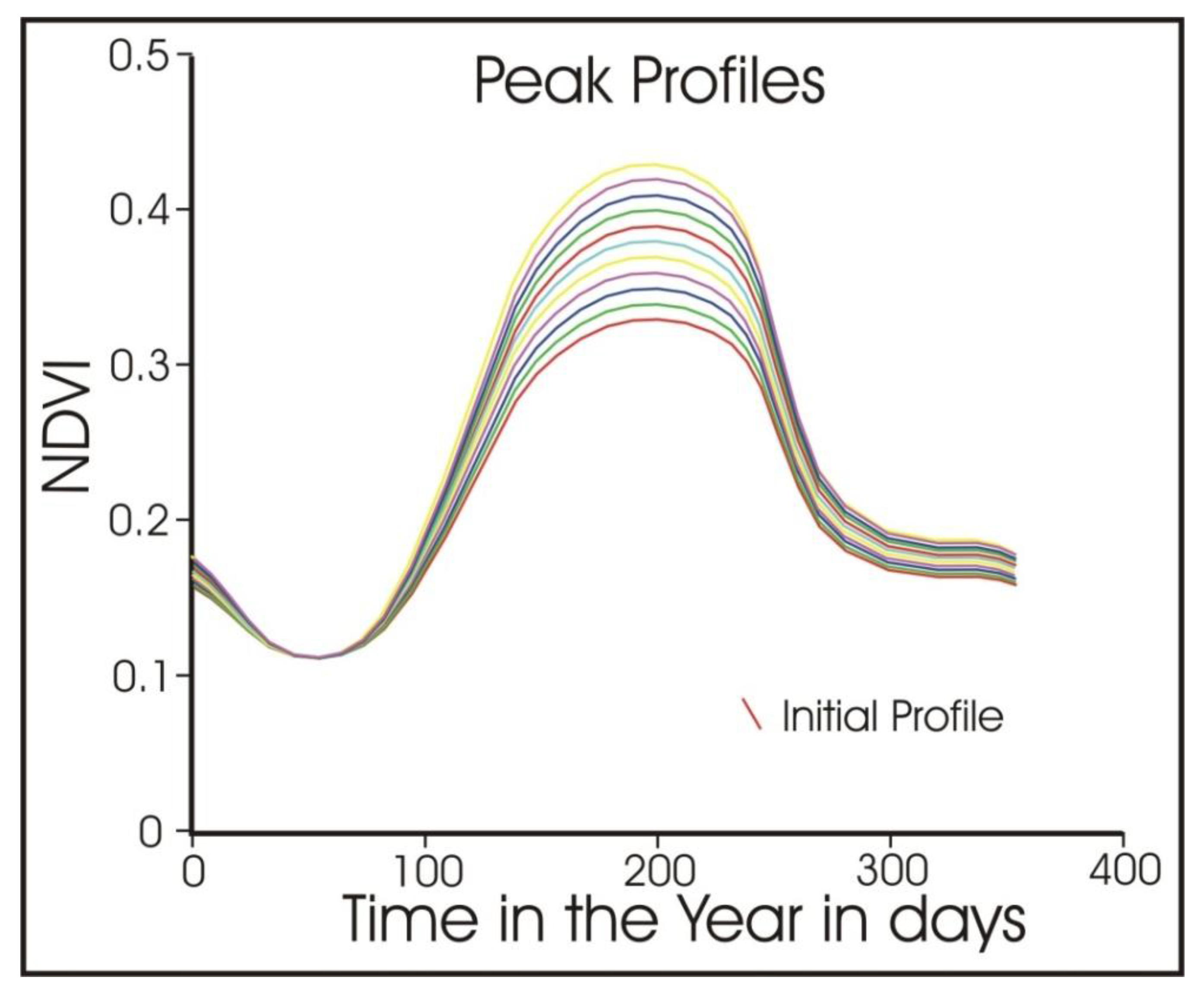
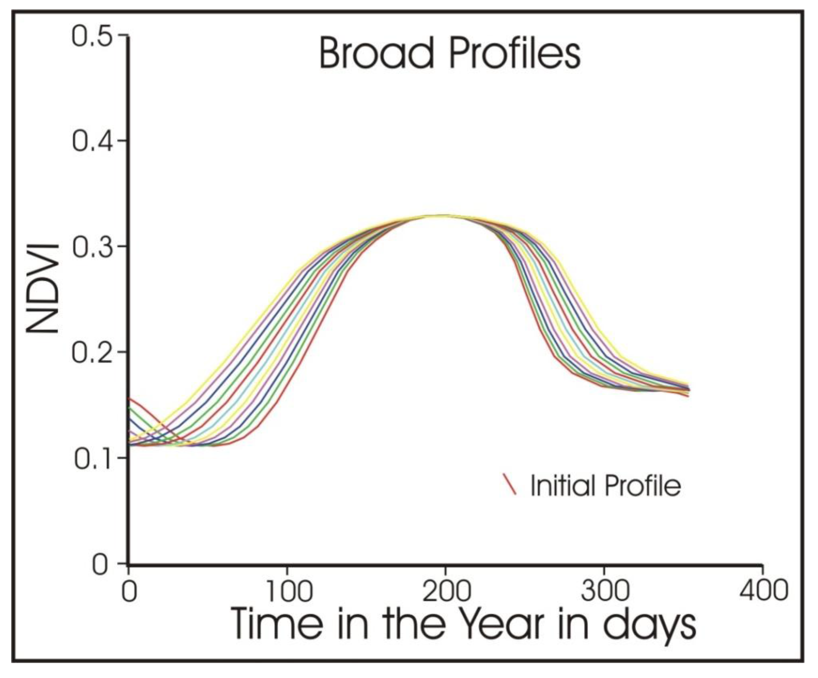
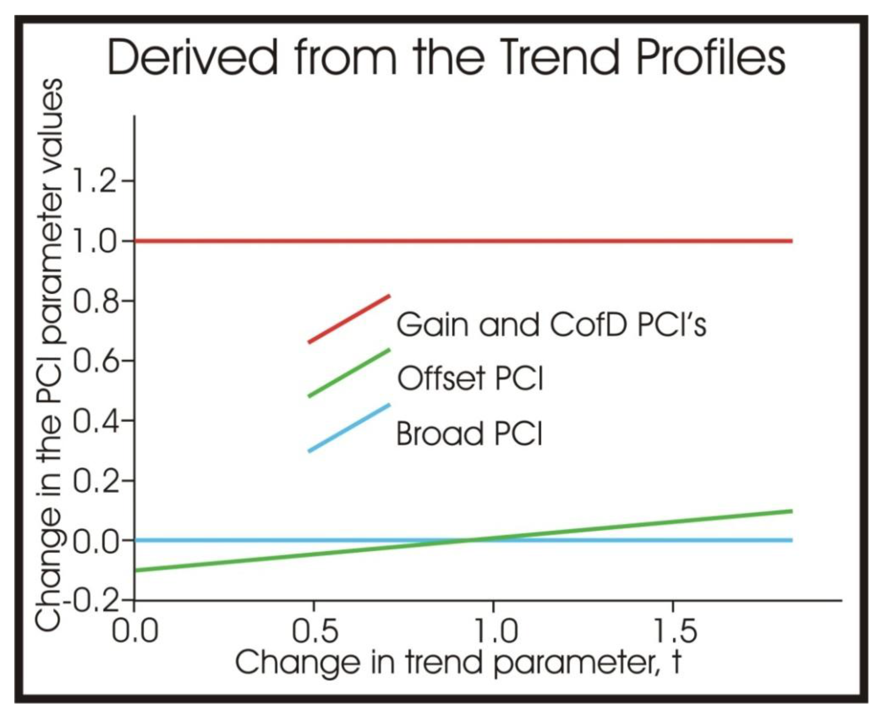
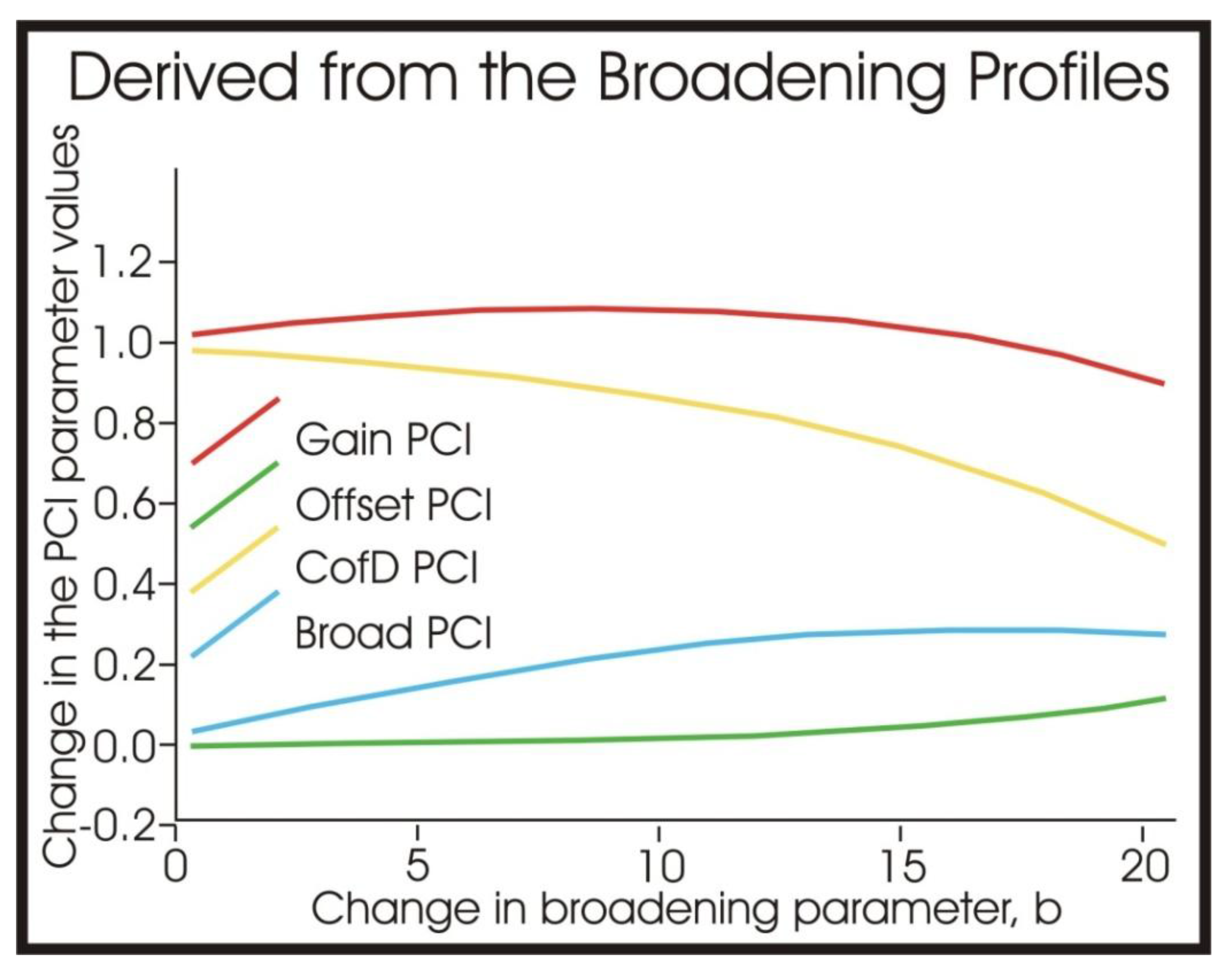
The author has developed and evaluated the characteristics of a set of six interrelated Phenological Change Indices which are designed to track the five ways in which it is considered that the phenological profile can change with time. A simulation study was conducted to verify how varying three factors will affect the phenologies of selected covers and the corresponding changes in the Phenological Change Indices. This study shows that the PCIs do closely track the changes that they are meant to measure, but that they can also change subtly with other types of change in the phenology. As a consequence, care needs to be taken in the interpretation of the indices. It is also clear that the changes detected by the Phenological Change Indices are a function of the starting conditions. As a consequence, many forms of analysis of these PCIs should proceed in conjunction with data on the land covers at the start of the time series used in the analysis.

The regional and land cover differences in phenological change strongly suggest that different land covers respond quite differently to climate change and that local driving mechanisms often dominate the effects of the global mechanisms in affecting the phenological profile. Some of these regional changes in phenology will be human induced and, as a consequence, there is a need to better understand how much of these detected changes are due to man, to climate, and due to man’s response to climate change.

None the less, understanding how global vegetation is responding to its forcing mechanisms in the face of climate change is crucial for a number of reasons. It has been shown [3] that changes in phenology can affect other physical parameters including evapo-transpiration, albedo, carbon fixation and nutrient cycling. Equally important is the need to track changes in the distribution of species in response to climate change: it has been noted by others [6] that changes in species condition and distribution can be abrupt and thus potentially catastrophic. The earlier we detect such abrupt changes, the earlier we can respond, both to inform society about the changes and to thus retain the trust and confidence of society, but also to look for appropriate remedial responses. A critical function of the remote sensing of vegetation is thus to detect changes in vegetative status as soon as possible so as to provide the appropriate resource managers with the best chance possible of making the optimal choice of alternative remedial responses.

This paper has shown that the analysis of trends does not capture all of the ways that vegetation phenology can change and as such it may either only provide a partial glimpse into the process or it may lead to erroneous conclusions. Some detected changes may arise due to several different causes. This paper has also shown that the individual phenological metrics are likewise limited in their usefulness; if one is to use phenological metrics as the basis for measuring changes in phenology, then a complementary set that measures all the ways that the phenology can change must be selected if the analyst wishes to draw rigorous conclusions about the nature of the changes that are taking place.

In this context it is realistic to ask whether these Phenological Change Indices identify any areas that appear to be significantly changing in a negative way; where a negative change would include a decline in amplitude, a decline in the average NDVI and a reduction in the duration of the season. There is only one area of a substantial size, in Western Tibet, that seems to fit these criteria from this data, although there are a number of individual pixels that meet these criteria.