Article

Phenological Classification of the United States: A Geographic Framework for Extending Multi-Sensor Time-Series Data

1
ASRC Research & Technology Solutions, Contractor to US Geological Survey Earth Resources Observation and Science Center, 47914 252nd Street, Sioux Falls, SD 57198, USA
2
US Geological Survey Earth Resources Observation and Science Center, 47914 252nd Street, Sioux Falls, SD 57198, USA
3
Department of Natural Resources and Environmental Management, University of Hawaii, 1910 East-West Road, Honolulu, HI 96822, USA
4
School of Natural Resources and the Environment & School of Geography and Development, University of Arizona, Tucson, AZ 85721, USA
5
US Geological Survey, 12201 Sunrise Valley Drive, Reston, VA 20192, USA
*
Author to whom correspondence should be addressed.
Remote Sens. 2010, 2(2), 526-544; https://doi.org/10.3390/rs2020526
Submission received: 22 December 2009 / Revised: 3 February 2010 / Accepted: 3 February 2010 / Published: 11 February 2010

Abstract

:
This study introduces a new geographic framework, phenological classification, for the conterminous United States based on Moderate Resolution Imaging Spectroradiometer (MODIS) Normalized Difference Vegetation Index (NDVI) time-series data and a digital elevation model. The resulting pheno-class map is comprised of 40 pheno-classes, each having unique phenological and topographic characteristics. Cross-comparison of the pheno-classes with the 2001 National Land Cover Database indicates that the new map contains additional phenological and climate information. The pheno-class framework may be a suitable basis for the development of an Advanced Very High Resolution Radiometer (AVHRR)-MODIS NDVI translation algorithm and for various biogeographic studies.

1. Introduction

Phenology is the study of the timing of recurring biological events [1] and examines the causes and consequences of biotic and environmental interactions. Phenology is usually influenced by photoperiod, precipitation, soil and air temperature, solar illumination, and other life-controlling factors [2,3,4]. The phenology of ecosystems and its connection to climate is a key to understanding ongoing global climate and land surface changes [5]. Phenology has historically been studied using ground-based observations of the timing of vegetation and animal pheno-phases such as germination, flowering, hibernation, and bird migration. Satellite observations provide continuous spatial and temporal coverage enabling scientists to assess and model seasonal dynamics and phenological variability of landscapes across large areas [6,7,8,9,10,11,12,13,14,15,16]. Time series of NDVI data derived from visible red and near-infrared bands [17] have been used to calculate phenological metrics [12,13,15,18].
Regionalization is a geographic or spatial type of classification that identifies, generalizes, and maps landscape patterns [19,20]. The outcome of regionalization is a geographic framework that reduces the complexity of the domain to something that is more manageable and understandable. For example, the United States has been subdivided into ecoregions [21,22]. The United States was also classified into land cover classes by the National Land Cover Database (NLCD) [23] using Landsat Thematic Mapper data. Both approaches produced very different geospatial characterizations of the same landscape, and both have proven to be valuable to the user community. Yet another way to subdivide, generalize, and characterize landscapes is by using phenology. Recently, White et al. [24] developed a global pheno-region database as a geographic framework for studying global climate change. White et al. [24] used 8-km AVHRR time series NDVI data (1982–1999) in conjunction with an eight-element monthly global climatology to generate global pheno-regions representing regions with a minimized probability of non-climatic forcing. Hargrove et al. [25] recently derived 15 phenological ecoregions based on clustering the similarities in five years (2002–2006) of cumulative MODIS NDVI data. Each year consists of 22 cumulative NDVI images based on the 23 composite periods per year.
AVHRR NDVI data have been proven to be valuable inputs for operational monitoring (e.g., fire danger monitoring, phenology, and drought) [12,26,27]. Although the MODIS mission (aboard Aqua and Terra platforms) is primarily research oriented, a similar opportunity exists to use these data streams for monitoring [28,29]. MODIS data have high spectral and spatial resolutions and provide an important bridge to the upcoming Visible/Infrared Imager Radiometer Suite (VIIRS) mission [30,31] because of the very similar radiometric characteristics between these two sensors. Characterizing multi-sensor long-term time-series vegetation index data and cross-sensor continuity is important [32] for monitoring climate impacts on vegetation response (e.g., vegetation drought monitoring). Satellite vegetation monitoring often relies on establishing baselines from NDVI time series to measure seasonal and interannual variability as deviations (or anomalies) from the established baselines [7,27,33].
Phenological classification, which characterizes and stratifies the land surface based on similar phenological patterns, may be a logical choice and suitable basis for a multi-sensor (e.g., AVHRR-MODIS) NDVI data translation algorithm to seamlessly extend the U.S. NDVI data record. This translation algorithm considers interannual variability and seasonality of biotic responses to adjust the cross-sensor continuity translation equations and requires information about the spatial heterogeneity of a representative range of land surfaces. The translation algorithm will be based on each pheno-class and will be used to extend the MODIS data record back to 1989 by tying it to the AVHRR NDVI data record. The resulting extended time series can be implemented within an operational vegetation drought monitoring system [33]. Here, we use the term “pheno-classes” to describe the regions identified by similar phenological patterns. These pheno-classes have unique spectral and temporal signatures.
The main goal of this study is to introduce a new geographical framework that identifies a set of regions with similar phenological patterns (or pheno-classes) based on land surface phenological metrics (timing and magnitude of NDVI) and elevation gradients. A similar approach by Hargrove [25] created fewer pheno-classes and is based on statistical clustering of five years of seasonal cumulative NDVI values without using explicit timing metrics. We first describe the methodology for generating the pheno-class map for the conterminous United States. Then we evaluate the characteristics of the new pheno-class map by comparing it to the 2001 NLCD land cover map [23].

2. Study Area and Datasets

This study focused on the conterminous United States and used MODIS 16-day 1-km surface reflectance data (MOD43B4, Collection 4) for generating phenological variables and developing of the pheno-class map. The MODIS surface reflectance data were obtained from the Land Processes Distributed Active Archive Center [34]. NDVI values were calculated according to the following equation:
N D V I = ρ N I R ρ Re d ρ N I R + ρ Re d
where ρRed and ρNIR are the reflectance values for MODIS bands 1 (620–670 nm) and 2 (841–876 nm), respectively. The 16-day NDVI composites were sequentially stacked to generate a five-year (2000–2004) time series. NDVI time-series data were filtered by the band quality flags and then smoothed (i.e., filtered) using a weighted least-squares approach to reduce any residual atmospheric noise [35].
Because elevation and corresponding vegetation gradients strongly influence phenological cycles [36,41], we incorporated a USGS 1-km DEM data for the conterminous United States to characterize topographic effects in our phenological classification. Land cover type data were obtained from the 2001 NLCD [23], which is based on multiple Landsat data transforms, elevation data, and ancillary data at a nominal resolution of 30 m. A 1-km ecoregion map generated from the Omernik level III ecoregion data [21] was compared with the newly developed pheno-class map. The ecoregion framework divides the landscape into a series of geographic regions with similar ecosystems and environmental resources that were identified using both biotic (e.g., vegetation and wildlife) and abiotic (e.g., climate, geology, hydrology, land use, and physiography) criteria.

3. Methodology

Our phenological classification methodology for the conterminous United States consisted of three steps. First, nine phenological metrics were derived from the five years (2000–2004) of 1-km MODIS NDVI data. We used software developed at the USGS Earth Resources Observation and Science (EROS) Center to calculate these metrics. Second, principal component analysis (PCA) was applied to the derived metrics and elevation values using ENVI software (ITT visual Information Solutions). Finally, iterative self-organizing data analysis (ISODATA) clustering was performed on the six principal component (PC) bands to generate the pheno-class map.

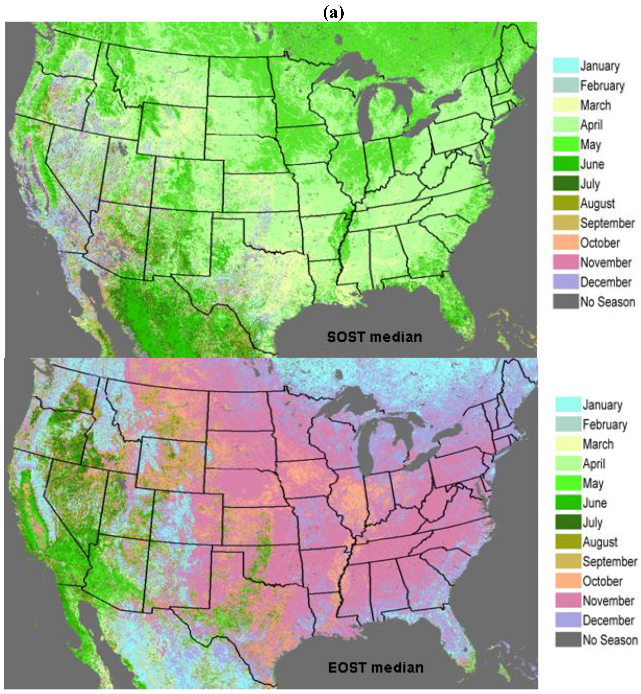
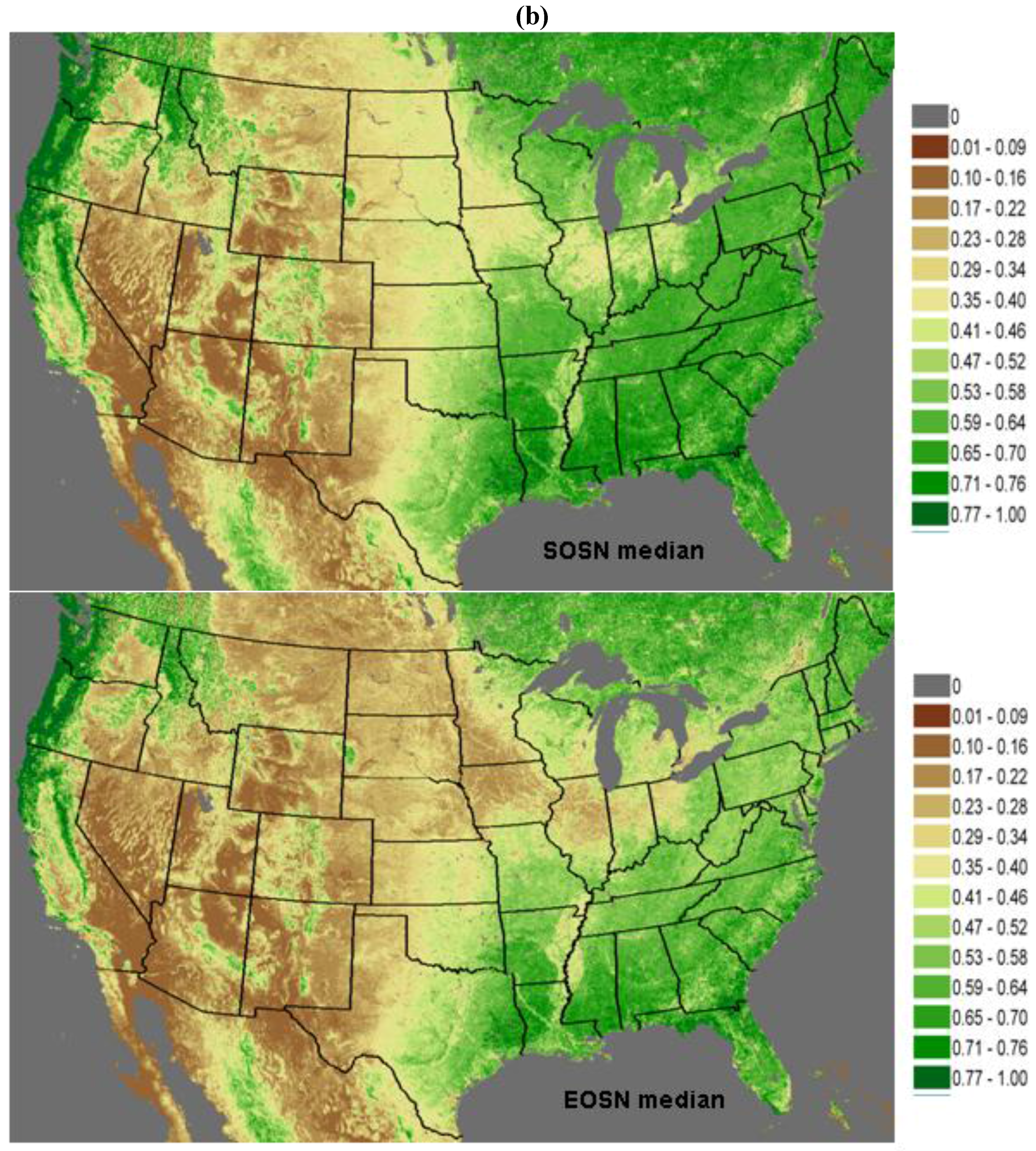
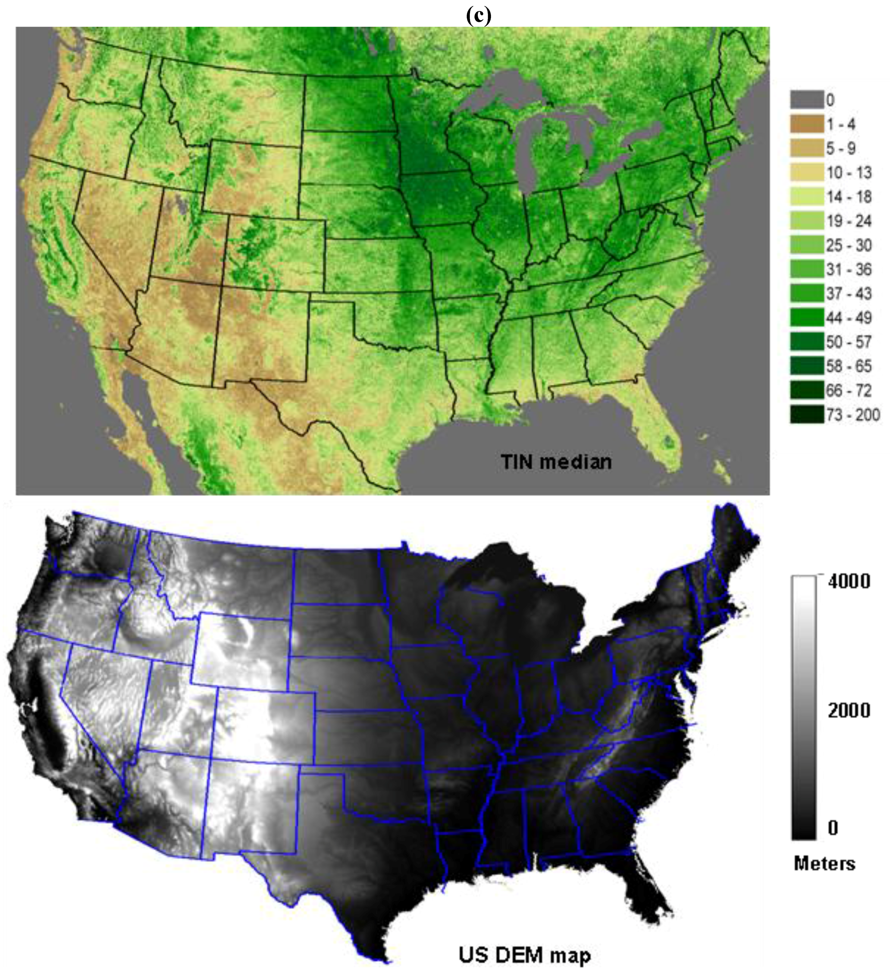
3.1. Derivation of Phenological Metrics

Land surface phenological variables were calculated based on the seasonality of the NDVI time-series data using a delayed moving average (DMA) method [12,13]. The nine phenological metrics used in the analysis were start-of-season time (SOST), start-of-season NDVI (SOSN), end-of-season time (EOST), end-of-season NDVI (EOSN), maximum NDVI (MAXN), maximum NDVI time (MAXT), duration of season (DUR), amplitude of NDVI (AMP), and seasonal time integrated NDVI (TIN). To reduce noise and missing values (e.g., where no start of season was identified in the data) and to characterize the “normal” phenology of the land surface, we calculated median values from the five years of data for each of the phenological metrics.

3.2. Data Normalization and Principal Component Analysis

Because of the large variability of the units and ranges of the nine phenological metrics and DEM data (e.g., the data for SOST ranges from 0 to 365 days and the data for the DEM ranges from 0 to 14,018 ft), data normalization for the nine phenological metrics and the DEM data was necessary to allow these datasets to be comparable (i.e., in a similar scale). This also resulted in a more even contribution of each input data layer into the principal component analysis. All input variables were transformed to comparable units using a z-score:
z s c o r e = x x ¯ σ
where x, x ¯ , and σ represent each data value, dataset mean, and dataset standard deviation, respectively.
In order to reduce noise and data dimensionality, we used PCA to generate new uncorrelated PC variables for clustering [37]. The PC bands with very low eigenvalues usually represent less data variance and more noise associated with the original data. In our analysis, the first six PC bands that contained more than 99% of the total variance were subsequently used in our classification. Regions of water and areas outside of the conterminous United States were masked out in the six PC bands.

3.3. Pheno-Class Derivation Using Unsupervised Isodata Technique

The ISODATA unsupervised classification is a widely used clustering technique that classifies all pixels based on iteratively recalculating the cluster means [38]. In this study, we applied the ISODATA classification method to generate the pheno-class map for the conterminous United States. Since the number of classes created by ISODATA is a user specified input, criteria to determine that number are helpful. We tested different numbers of pheno-classes (e.g., 25, 30, 40, and 50) to determine the optimum number of pheno-classes.

3.4. Evaluation of Derived Pheno-Class Map

To evaluate the final U.S. pheno-class map, we compared it to the 2001 NLCD map [23] and the Omernik ecoregions map [21] and computed Minnick’s coefficients to assess the degree of overlap between the pheno-classes and vegetation cover classes. Minnick’s coefficient (Cm), which represents the fraction of how much two classes overlap to overall union of the two classes, is also calculated to identify individual class associations [39,40]:
C m = A B A B ( A B )
where AB is the intersection of classes A and B (common area), and AB is the union of A and B (areas in A or B as well as areas in both A and B).

4. Results and Discussions

4.1. Examples of the Five-Year Median Phenological Metric Maps

Figure 1 shows some examples of key phenological metrics (SOST, EOST, SOSN, and EOSN) and the DEM map used to generate the pheno-classes. Specific phenological and DEM patterns within the conterminous United States are apparent in Figure 1. For example, the median start-of-season time for the winter wheat region in Oklahoma and Texas is commonly in December, and the end-of-season time for this region ranges from May to June.

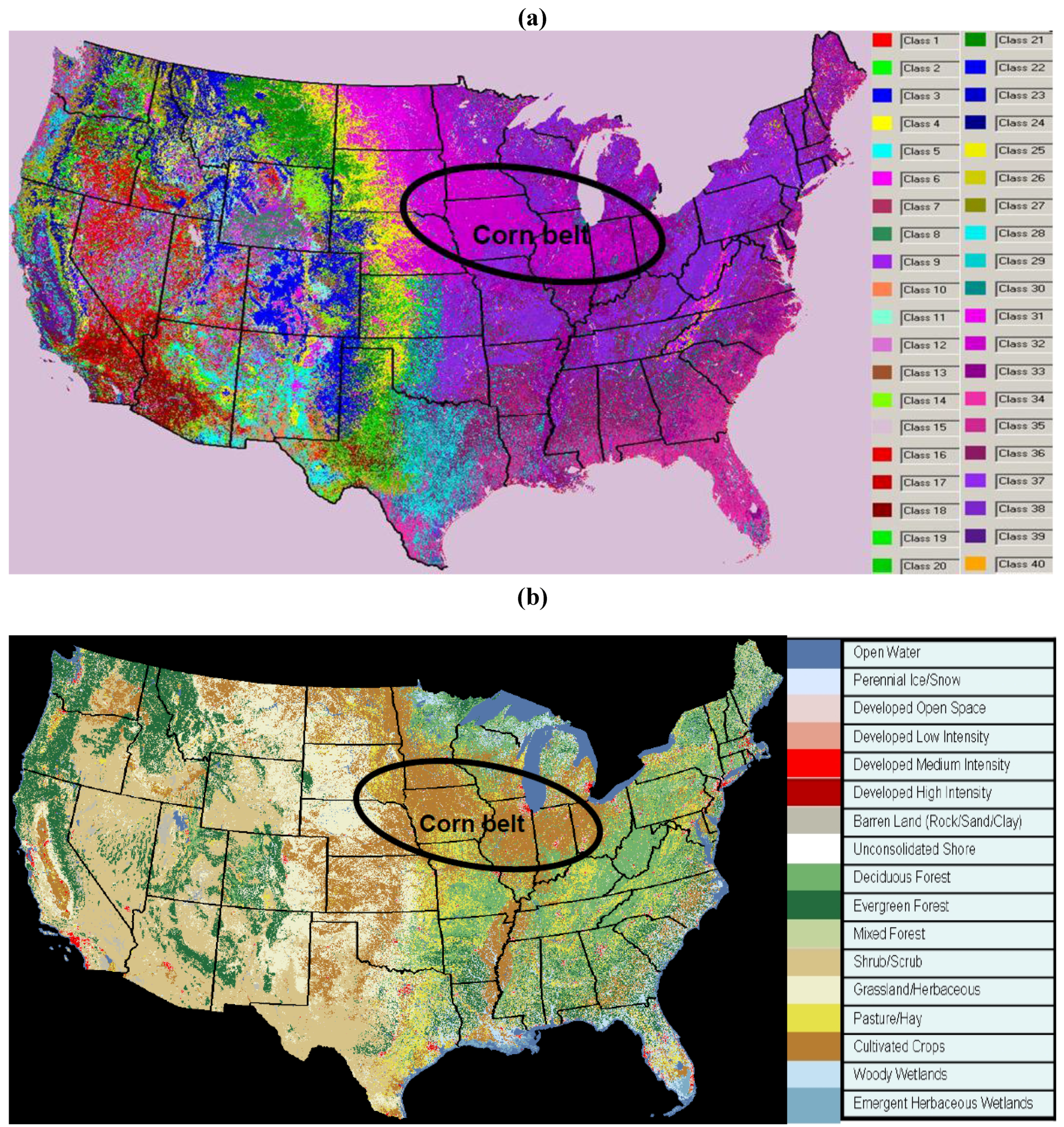
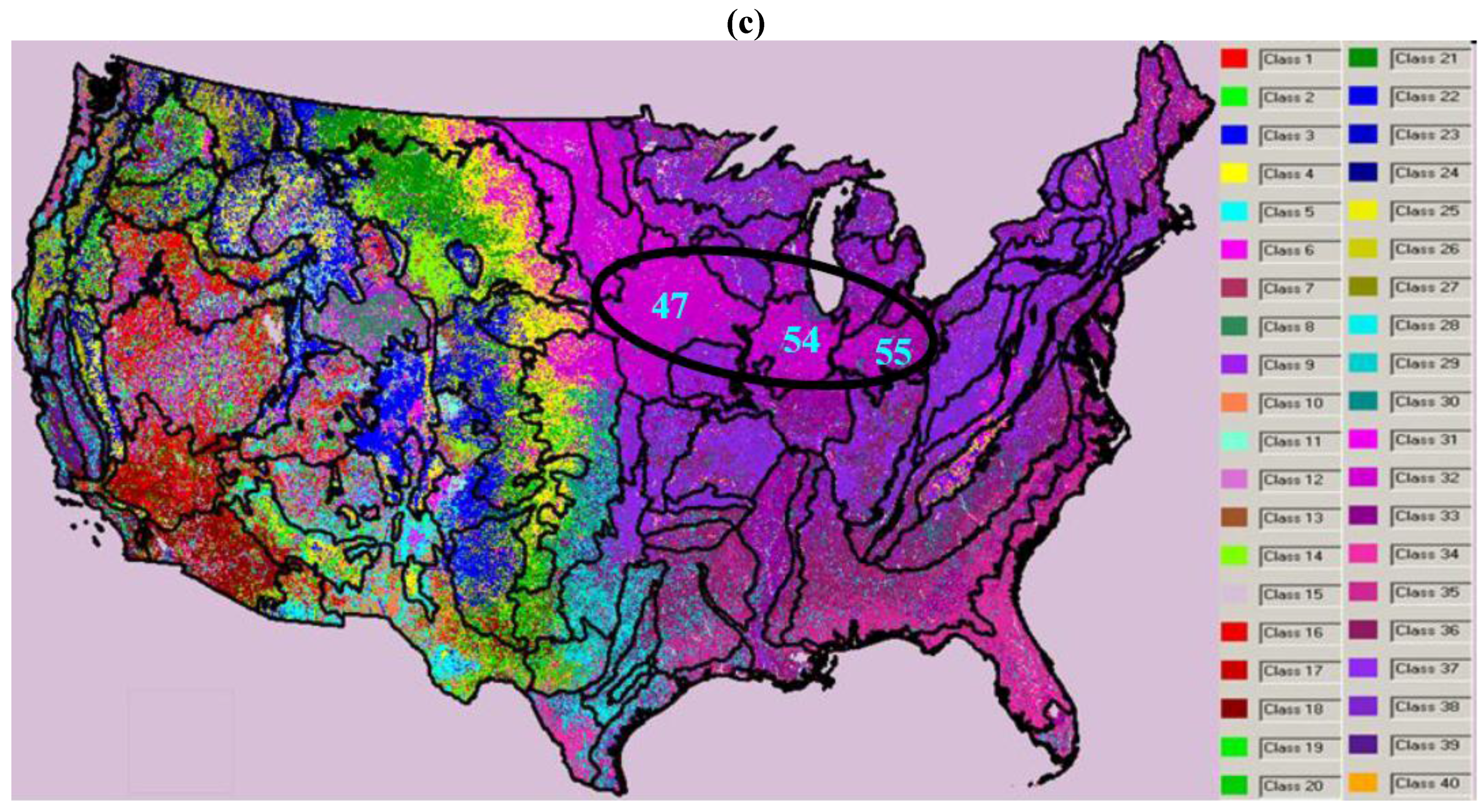
4.2. Pheno-Class Map for the Conterminous United States

Iterative testing of the number of pheno-classes indicated that many isolated points existed in the western United States in the ISODATA classification when the number of pheno-classes approached 50. Conversely, only 3–4 pheno-classes represented the eastern United States if the target number of pheno-classes was less than 30. Based on the existing land cover patterns (2001 NLCD map) and above testing criteria (visually and qualitatively by balancing the number of phenoclasses in the United States), we decided to use 40 pheno-classes within the conterminous United States for this study. Figure 2 shows the final 40 pheno-classes for the conterminous United States (one pheno-class is the background) compared with the 2001 NLCD map and U.S. ecoregions map. A noticeable feature is the comparatively high number of classes located in the western half of the United States compared to the east. A likely explanation for these two contrasting spatial patterns is the relatively large variability in elevation and climate in the western United States. Elevation and corresponding vegetation gradients strongly affect phenological cycles [36,41].
Visual comparisons between the phenological framework derived classes and the 2001 NLCD land cover classes show a number of similarities and differences. For example, the Midwestern corn belt, a region that is distinguished by both phenological and agricultural homogeneity, is similar in both datasets. Conversely, differences can be seen for the conifer forest class. As depicted by NLCD, conifer forest is found across large geographic space and thrives in different environmental and climate niches (e.g., southeastern loblolly pine forest and southwestern pinyon-juniper forest). Our results show that this one NLCD land cover class (i.e., conifer forest) contains multiple pheno-classes. The results from our intercomparison and Minnick’s coefficients in the next sections provide some insights into the correspondence between pheno-classes and land cover classes (NLCD).
Figure 1. Examples of phenological metrics maps derived from MODIS NDVI time-series data between 2000 and 2004. The DEM was used as a proxy for climate. (a) SOST and EOST; (b) SOSN and EOSN; (c) TIN and DEM maps.
Remotesensing 02 00526 g001aRemotesensing 02 00526 g001bRemotesensing 02 00526 g001c
Figure 2. US pheno-class map derived from the median of the 5-year (2000–2004) of phenological metrics. The 2001 NLCD map was used to guide the number of ISODATA classes. (a) US pheno-class map; (b) 2001 NLCD map; (c) US ecoregion map delineated on the US pheno-class map in black.
Remotesensing 02 00526 g002aRemotesensing 02 00526 g002b
Figure 3. Mean values of nine phenological metrics and the DEM data for representative pheno-classes 7, 17, 27, and 37. The nine phenological metrics included start-of-season time (SOST), start-of-season NDVI (SOSN), end-of-season time (EOST), end-of-season NDVI (EOSN), maximum NDVI (MAXN), maximum NDVI time (MAXT), duration of season (DUR), amplitude of NDVI (AMP), and seasonal time integrated NDVI (TIN). (a) NDVI-based phenological metrics; (b) timing-based phenological metrics and DEM.
Remotesensing 02 00526 g003aRemotesensing 02 00526 g003b
Some examples of the unique phenological and DEM features for several random selected pheno-classes (i.e., pheno-classes 7, 17, 27, and 37) are shown in Figure 3. The mean values for nine phenological metrics and DEM show both the characteristics and the basis for separating these classes in this geographic framework. More in-depth analysis results for certain pheno-classes will be presented in section 4.4.
Visual comparisons between the pheno-class map and the U.S. ecoregions were performed in this study. The ecoregions within the conterminous United States are delineated in black on the pheno-class map in Figure 2c. Results show both the consistency and the differences between these two maps. For example, pheno-class 32, which represents the Midwestern corn belt in the pheno-class map, is related to ecoregions 47 (Western Corn Belt Plains), 54 (Central Corn Belt Plains), and 55 (Eastern Corn Belt Plains), demonstrating the consistency of these two maps. On the other hand, many ecoregions contain multiple pheno-classes (Figure 2c), revealing the differences between these two frameworks.

4.3. Intercomparison of Pheno-Class and Land Cover

To provide further explanation of the phenological classes, we performed an intercomparison between the pheno-class map and the 2001 NLCD. The concurrent geographic overlaps for the two systems (i.e., the percentage of land cover types in each pheno-class) are listed in Table 1. Percentage ranges 26–50%, 51–75%, and 76–100% are highlighted in yellow, aqua, and pink, respectively. Results from Table 1 demonstrate again that one land cover type will be represented by many different pheno-classes. For example, the main land cover type for pheno-classes 8 and 17 is shrub/scrub cover (~80% for each pheno-class). However, these two pheno-classes have distinctly different phenological and elevational characteristics (Figure 4). The geographic locations of these two pheno-classes are also shown in Figure 4. This illustrates how a single land cover class can exhibit multiple phenological responses to environmental conditions, climate variability, plant communities, and topography. As a result of these differences, pheno-classes 8 and 17 (scrub/shrub cover) are separated from each other by this methodology. We deduce that the pheno-class map provides unique information that can augment that provided by the 2001 NLCD map.
Table 1. Each pheno-class represents a range of different land cover types, which are expressed as a percentage of each coinciding land cover area over the total pheno- class area. Percentage ranges 26–50%, 51–75%, and 76–100% are highlighted in yellow, aqua, and pink, respectively.
Land cover/Pheno-classOpen WaterPerennial Ice/SnowDeveloped, Urban areaBarren Land (Rock/Sand/Clay)Deciduous ForestEvergreen ForestMixed ForestShrub/ScrubGrassland/HerbaceousPasture/HayCultivated CropsWoody WetlandsEmergent Herbaceous Wetlands
10.00.010.49.414.413.13.14.35.43.95.67.622.4
20.00.10.43.70.038.10.151.54.90.20.80.10.1
30.00.40.14.414.549.91.114.312.81.50.00.50.3
40.00.10.31.80.675.70.114.26.80.20.00.10.1
50.00.00.72.90.09.80.066.219.00.30.90.10.1
60.00.00.91.50.622.10.048.723.81.30.30.30.5
70.00.10.21.20.236.70.051.29.50.40.30.10.1
80.00.00.10.40.110.40.081.26.60.40.30.10.3
90.00.00.22.40.04.20.083.19.10.40.30.10.1
100.00.01.16.10.01.60.070.418.00.61.60.30.2
110.00.00.40.35.730.10.238.220.32.80.70.50.9
120.00.00.22.30.011.00.078.07.20.40.70.10.1
130.00.00.60.30.310.50.147.531.32.56.20.40.4
140.00.00.60.60.03.40.035.848.21.69.10.30.3
157.40.00.00.00.00.00.00.20.00.00.00.00.0
160.00.00.34.30.02.10.180.410.20.51.80.10.1
170.00.00.24.20.08.40.179.46.10.41.10.10.1
180.00.04.34.80.23.30.574.55.90.95.10.30.3
190.00.00.70.30.34.60.437.223.31.131.90.10.2
200.00.03.32.30.27.00.358.717.40.59.90.20.2
210.00.00.70.60.12.00.020.156.20.619.20.30.2
220.00.01.40.30.04.00.019.351.41.820.70.50.5
230.00.00.80.44.337.30.115.015.57.117.11.31.2
240.00.10.50.80.372.90.212.24.20.38.20.10.2
250.00.00.70.22.22.40.15.461.02.824.20.50.5
260.00.01.50.90.438.00.542.15.20.310.90.20.1
270.00.00.80.23.769.62.517.23.30.91.20.70.2
280.00.04.80.42.112.32.525.716.512.320.22.01.3
290.00.08.20.36.216.53.414.114.117.810.57.41.4
300.00.014.40.49.94.90.98.518.813.424.53.11.0
310.00.00.80.113.82.20.90.933.88.836.31.01.3
320.00.01.00.14.80.30.10.13.37.180.11.21.9
330.00.05.40.215.95.12.41.12.513.945.56.61.5
340.00.09.91.31.217.80.926.07.77.711.310.95.2
350.00.05.70.46.636.05.87.05.88.07.615.02.2
360.00.05.80.226.114.75.24.04.023.16.19.71.1
370.00.04.50.146.33.83.50.96.020.48.55.60.5
380.00.01.60.158.22.22.40.66.110.511.95.01.4
390.00.02.70.80.61.31.116.540.15.529.80.41.1
400.00.00.82.80.125.10.359.67.00.23.40.30.2
Figure 4. Mean values of the nine phenological metrics and the associated elevation data for pheno-classes 8 and 17. The geographic distributions of locations for these two pheno-classes are also shown in the figure. (a) NDVI-based phenological metrics; (b) timing-based phenological metrics and DEM.
Remotesensing 02 00526 g004
Table 2 provides the Cm values calculated for each combination of pheno-class and land cover class. Examination of the Cm values of 0.05 or higher (indicating a moderate to high spatial association) show that about half of the NLCD classes correlate with one to up to seven pheno-classes (Table 2). Many combinations showed lesser overlap between land cover and pheno-classes (0.02 < Cm < 0.05). Strong associations (Cm > 0.10) included values as high as 0.41 between cultivated crops and pheno-class 32. Cm values of 0.10 or higher occurred for pheno-classes correlating with deciduous forest, evergreen forest, shrub/scrub, grassland/herbaceous, pasture/hay, cultivated crops, and woody wetlands.
Table 2. Cm values show the degree of overlap for each combination of pheno-class and NLCD-based land cover class. Cm values ranges 0.02–0.05, 0.05–0.1, and 0.1–0.5 are highlighted in yellow, aqua, and pink, respectively.
Land cover/Pheno-classOpen WaterPerennial Ice/SnowDeveloped, Urban areaBarren Land (Rock/Sand/Clay)Deciduous ForestEvergreen ForestMixed ForestShrub/ScrubGrassland/HerbaceousPasture/HayCultivated CropsWoody WetlandsEmergent Herbaceous Wetlands
10.000.000.010.030.010.010.010.000.000.000.000.010.09
20.000.000.000.020.000.050.000.040.010.000.000.000.00
30.000.000.000.030.020.080.010.010.020.000.000.000.00
40.000.000.000.010.000.100.000.010.010.000.000.000.00
50.000.000.000.020.000.020.000.070.030.000.000.000.00
60.000.000.000.010.000.020.000.030.020.000.000.000.00
70.000.000.000.000.000.020.000.010.000.000.000.000.00
80.000.000.000.000.000.010.000.040.000.000.000.000.00
90.000.000.000.010.000.000.000.050.010.000.000.000.00
100.000.000.000.040.000.000.000.060.020.000.000.000.00
110.000.000.000.000.010.030.000.030.020.010.000.000.01
120.000.000.000.010.000.010.000.050.010.000.000.000.00
130.000.000.000.000.000.010.000.020.020.000.000.000.00
140.000.000.000.000.000.000.000.030.050.000.010.000.00
150.080.000.000.000.000.000.000.000.000.000.000.000.00
160.000.000.000.030.000.000.000.070.010.000.000.000.00
170.000.000.000.030.000.010.000.100.010.000.000.000.00
180.000.000.010.040.000.010.000.110.010.000.010.000.00
190.000.000.000.000.000.000.000.020.020.000.020.000.00
200.000.000.000.010.000.010.000.030.010.000.010.000.00
210.000.000.000.000.000.000.000.020.110.000.030.000.00
220.000.000.000.000.000.010.000.020.090.000.030.000.00
230.000.000.000.000.010.050.000.010.020.010.020.010.01
240.000.000.000.000.000.070.000.010.000.000.010.000.00
250.000.000.000.000.010.010.000.010.170.010.050.000.00
260.000.000.000.000.000.030.000.020.000.000.010.000.00
270.000.000.000.000.000.070.010.010.000.000.000.000.00
280.000.000.010.000.000.010.010.020.020.020.020.010.01
290.000.000.020.000.010.030.020.010.020.050.010.030.01
300.000.000.030.000.020.010.010.010.030.030.030.010.01
310.000.000.000.000.030.010.010.000.070.030.070.010.01
320.000.000.010.000.020.000.000.000.010.040.410.010.02
330.000.000.020.000.060.020.020.000.010.070.170.050.01
340.000.000.020.010.000.020.010.020.010.020.010.040.04
350.000.000.020.000.020.130.050.010.020.040.020.110.02
360.000.000.020.000.120.060.050.010.010.150.020.080.01
370.000.000.020.000.280.010.030.000.020.130.030.040.00
380.000.000.010.000.300.010.020.000.020.050.030.030.01
390.000.000.010.000.000.000.010.010.040.010.020.000.01
400.000.000.000.010.000.010.000.020.000.000.000.000.00

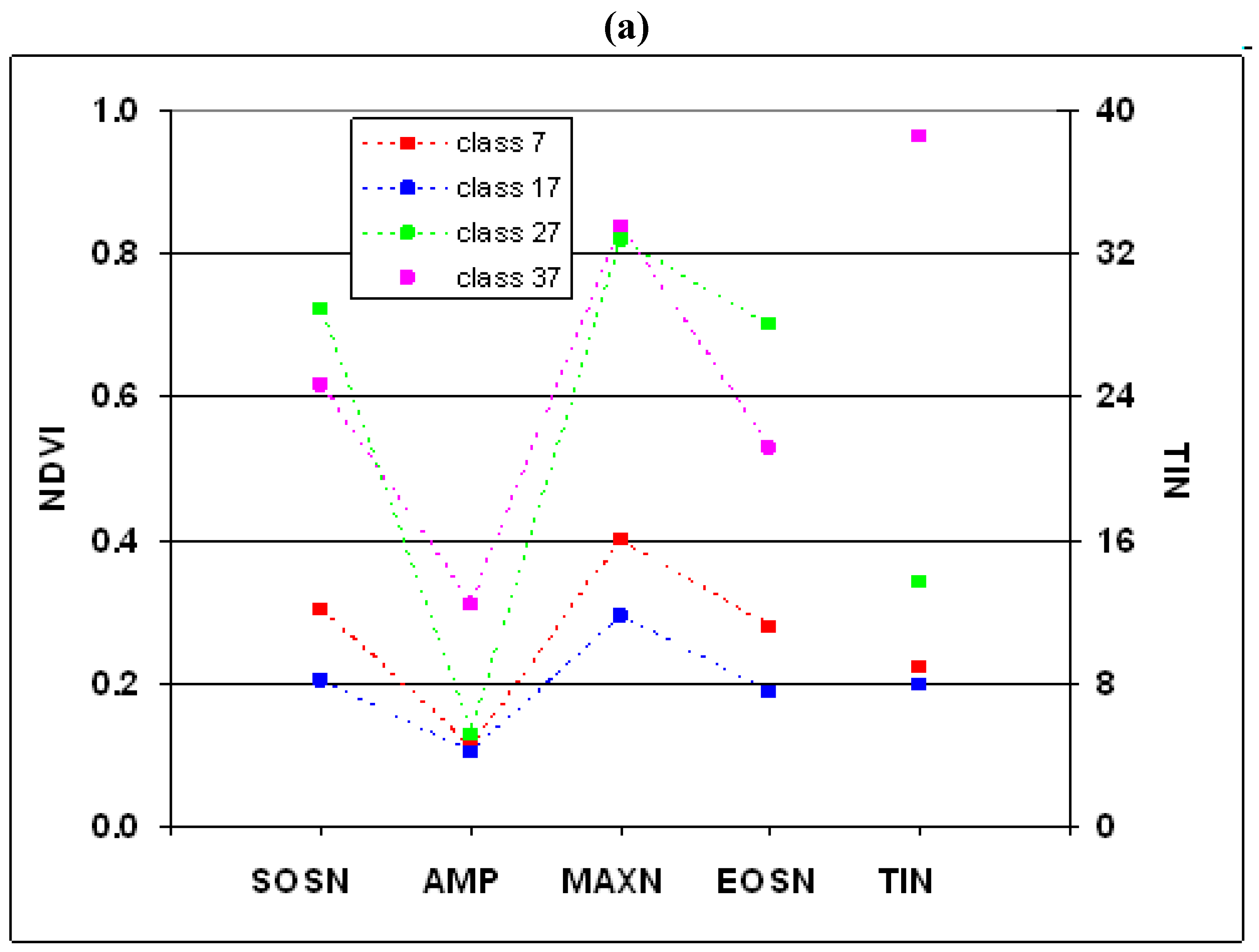
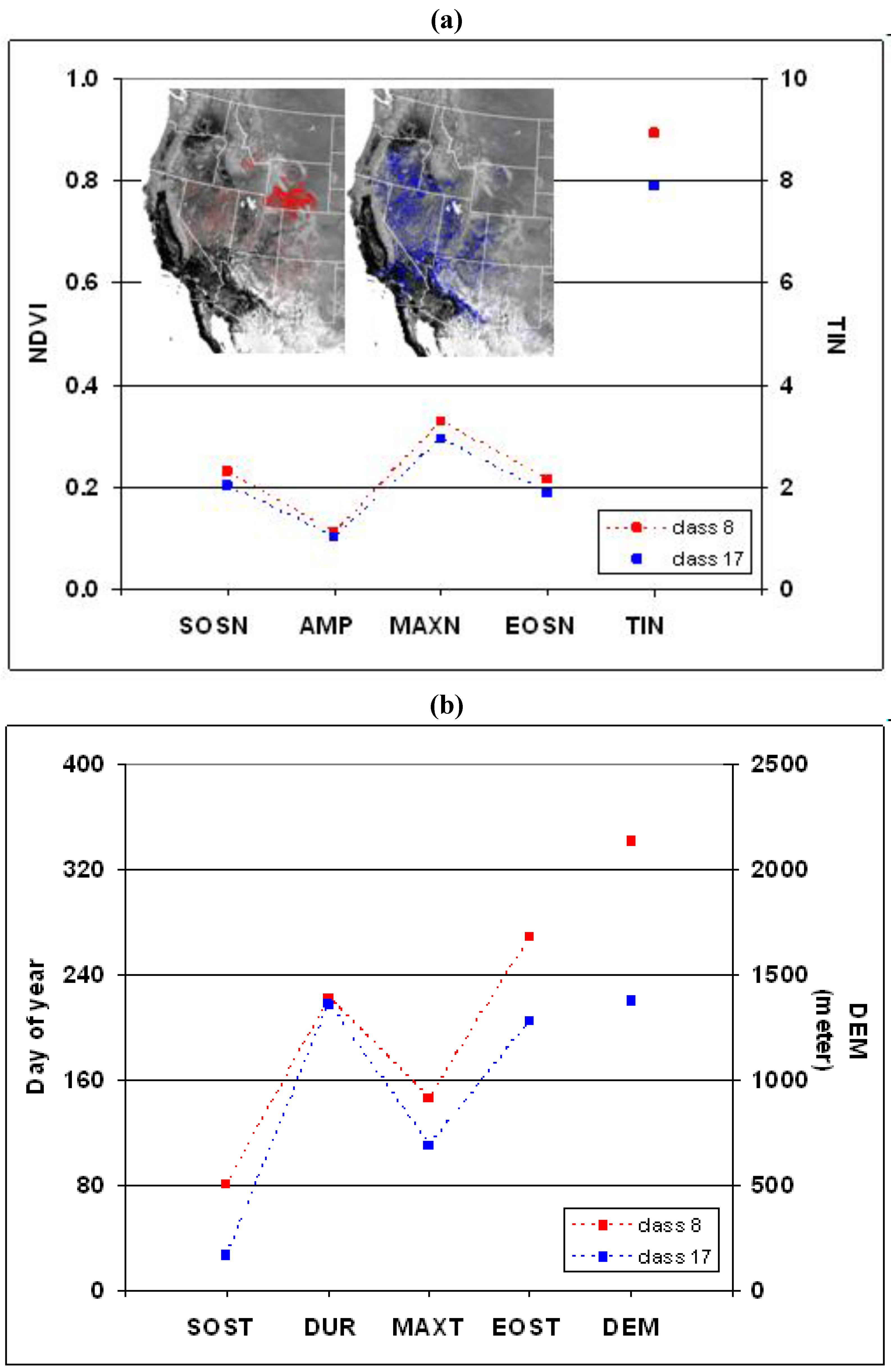
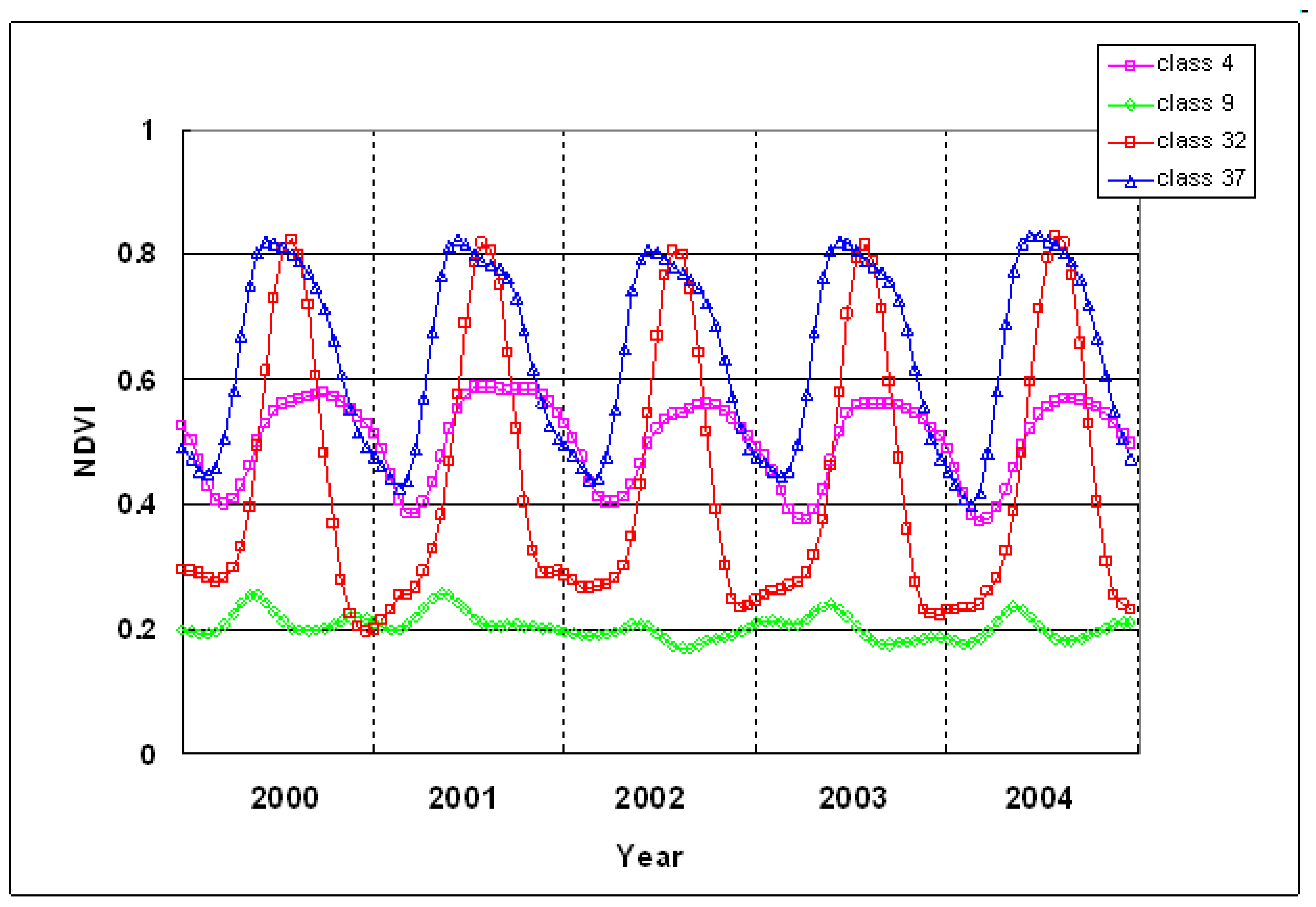
4.4. In-depth Analysis of Selected Pheno-Classes

Four representative pheno-classes (4, 9, 32, and 37) were chosen to further illustrate the basis of this geographic framework. The dominant land cover types (from the NLCD) for pheno-classes 4, 9, 32, and 37 are 76% evergreen forest, 83% shrub, 80% cultivated crops, and 46% deciduous forest and 20% pasture/hay, respectively. The mean non-normalized values of SOST, EOST, and TIN for these pheno-classes are plotted in Figure 5 as well as their geographic distributions. We evaluated the non-normalized SOST, EOST, and TIN to help describe the phenological and elevation characteristics of these representative pheno-classes. We found that pheno-class 9 has much lower TIN (<7) than pheno-classes 32 and 37 (>38). This suggests that less seasonal greenness magnitudes and variation of shrub cover resulted in a very low time integrated NDVI. On the other hand, pheno-classes 32 and 37 have much higher TIN due to the significant seasonal greenness variations typically found for crops and forest.
Figure 5. Mean values of SOST, EOST, and TIN for pheno-class 4 (pink, 76% evergreen forest, 14% shrub), pheno-class 9 (green, 83% shrub, 9% grassland), pheno-class 32 (red, 80% cultivated crops), and pheno-class 37 (blue, 46% forest, 20% pasture/hay). The geographic distributions of the locations for each pheno-class are highlighted with the corresponding colors in both graphs.
Remotesensing 02 00526 g005
The NDVI time-series (2000–2004) data for pheno-classes 4, 9, 32, and 37 (mean values) are presented in Figure 6 to further illustrate the phenological trajectories for these four pheno-classes. The mean start-of-season and end-of-season times for pheno-class 9 are earlier than for pheno-classes 32 and 37 (Figure 5). The duration of the season for pheno-class 37 is nearly one month longer than for pheno-class 32, indicating that forest (and grass) for this region has a longer growing season than agriculture. Pheno-class 4 (evergreen forest) showed the longest season (~10 months) (Figure 5).
Figure 6. Multi-year seasonal NDVI time-series trajectories (2000–2004) for representative pheno-classes 4, 9, 32, and 37 (spatially averaged NDVI values) show the different phenological patterns for each pheno-class.
Remotesensing 02 00526 g006

5. Conclusions

This study introduces a new geographic framework that is based on phenology and elevation characteristics. The new pheno-class map for the conterminous United States was generated based on nine phenological metrics derived from satellite MODIS NDVI and USGS DEM data. The pheno-class regionalization provided a geographic framework for multi-sensor data translation research because it provides information about the magnitude, timing, and spatial variability of biological phenomena. Compared to the 2001 NLCD map, the pheno-class map contained additional information about regional phenology and phenological spatial patterns.
The original proposed use for this pheno-class framework is to support the development of a pheno-class based AVHRR-MODIS NDVI translation algorithm to seamlessly extend our multi-sensor NDVI data record. Additional research to accomplish this is underway. However, we believe that the new pheno-class map described in this study will be useful for multiple purposes. These new pheno-classes can be used to further explore biogeographic patterns that may emerge as a result of diversification, migration, and extinction of species and communities in response to environmental changes and variability. The new pheno-class map may also have additional value as a regional framework for other research and applications related to land surface monitoring and assessment [9], including agricultural monitoring, real-time drought monitoring, ecological modeling of the impact of global changes [42] on biodiversity and invasive species, and biogeochemical modeling to assess carbon sequestration and impacts of climate on our dynamic environment.

Acknowledgements

This work was performed under USGS contract 08HQCN0007 and partially funded by the USGS Geographic Analysis and Monitoring Program. Additional support was provided by NASA grant MEaSUREs NNX08AT05A and EOS grant NNG04GL88G. The authors thank Bruce K. Wylie, James E. Vogelmann, and Michael P. Crane for their valuable suggestions and comments. Any use of trade, product, or firm names is for descriptive purposes only and does not imply endorsement by the US Government.

References

  1. Lieth, H. Purposes of a phenology book. In Phenology and Seasonality Modeling; Lieth, H., Ed.; Springer-Verlag: New York, NY, USA, 1974; pp. 3–19. [Google Scholar]
  2. Barnes, P.W.; Tieszen, L.L.; Ode, D.J. Distribution, production, and diversity of C 3-and C 4-dominated communities in a mixed prairie. Can. J. Bot. 1983, 61, 741–751. [Google Scholar] [CrossRef]
  3. Flint, H.L. Phenology and genecology of woody plants. In Phenology and Seasonality Modeling; Lieth, H., Ed.; Springer-Verlag: New York, NY, USA, 1974; pp. 83–97. [Google Scholar]
  4. Lewis, J.K. The grassland biome: A synthesis of structure and function, 1970. In Preliminary Analysis of Structure and Function in Grasslands; Range Science Series 10 N; French, R., Ed.; Colorado State University: Fort Collins, CO, USA, 1971; pp. 317–387. [Google Scholar]
  5. van Vliet, A.J.H.; Schwartz, M.D. Phenology and climate: The timing of life cycle events as indicators of climate variability and change. Int. J. Climatol. 2002, 22, 1713–1714. [Google Scholar] [CrossRef]
  6. Anderson, J.R.; Hardy, E.E.; Roach, J.T. A Land Use and Land Cover Classification System for Use with Remote Sensor Data; US Geological Survey Professional Paper P 0964; US Geological Survey: Reston, VA, USA, 1976.
  7. Gu, Y.; Brown, J.F.; Verdin, J.P.; Wardlow, B. A five-year analysis of MODIS NDVI and NDWI for grassland drought assessment over the central Great Plains of the United States. Geophys. Res. Lett. 2007, 34. [Google Scholar] [CrossRef]
  8. MacDonald, R.B.; Hall, F.G. Global Crop Forecasting. Science 1980, 208, 670–679. [Google Scholar] [CrossRef] [PubMed]
  9. Nemani, R.; Hashimoto, H.; Votava, P. Monitoring and forecasting ecosystem dynamics using the Terrestrial Observation and Prediction System (TOPS). Rem. Sens. Environ. 2009, 113, 1497–1509. [Google Scholar] [CrossRef]
  10. Peters, A.J.; Walter-Shea, E.A.; Ji, L. Drought monitoring with NDVI-based Standardized Vegetation Index. Photogramm. Eng. Rem. Sens. 2002, 68, 71–75. [Google Scholar]
  11. Reed, B.C. Using remote sensing and geographic information systems for analysing landscape/drought interaction. Int. J.Remote Sens. 1993, 14, 3489–3503. [Google Scholar] [CrossRef]
  12. Reed, B.C.; Brown, J.F.; Vanderzee, D. Measuring phenological variability from satellite imagery. J. Veg. Sci. 1994, 5, 703–714. [Google Scholar] [CrossRef]
  13. Reed, B.C.; White, M.A.; Brown, J.F. Remote sensing phenology. In Phenology: An Integrative Environmental Science; Schwartz, M.D., Ed.; Kluwer Academic Publishers: Dordrecht, The Netherlands, 2003; pp. 365–381. [Google Scholar]
  14. White, M.A.; de Beurs, K.M.; Didan, K. Intercomparison, interpretation, and assessment of spring phenology in North America estimated from remote sensing for 1982–2006. Global Change Biol. 2009, 15, 2335–2359. [Google Scholar] [CrossRef]
  15. White, M.A.; Thornton, P.E.; Running, S.W. A continental phenology model for monitoring vegetation responses to interannual climatic variability. Global Biogeochem. Cycle 1997, 11, 217–234. [Google Scholar] [CrossRef]
  16. Yang, L.; Wylie, B.K.; Tieszen, L.L. An analysis of relationships among climate forcing and time-integrated NDVI of grasslands over the U.S. northern and central Great Plains. Rem. Sens. Environ. 1998, 65, 25–37. [Google Scholar] [CrossRef]
  17. Tucker, C.J. Red and photographic infrared linear combinations for monitoring vegetation. Rem. Sens. Environ. 1979, 8, 127–150. [Google Scholar] [CrossRef]
  18. Jönsson, P.; Eklundh, L. Seasonality extraction by function fitting to time-series of satellite sensor data. IEEE Trans. Geosci. Rem. Sens. 2002, 40, 1824–1832. [Google Scholar] [CrossRef]
  19. Chorley, R.J.; Haggett, P. Models in Geography; Methuen: London, UK, 1967. [Google Scholar]
  20. Johnson, A.F. A Programmed Course in Cataloguing and Classification; Deutsch: London, UK, 1968. [Google Scholar]
  21. Omernik, J.M. Ecoregions of the conterminous United States. Ann. Assoc. Am. Geogr. 1987, 77, 118–125. [Google Scholar] [CrossRef]
  22. Bailey, R.G.; Hogg, H.C. A world ecoregions map for resource reporting. Environ. Conserv. 1986, 13, 195–202. [Google Scholar] [CrossRef]
  23. Homer, C.; Huang, C.; Yang, L. Development of a 2001 National Land-Cover Database for the United States. Photogramm. Eng. Rem. Sens. 2004, 70, 829–840. [Google Scholar] [CrossRef]
  24. White, M.A.; Hoffman, F.; Hargrove, W.W. A global framework for monitoring phenological responses to climate change. Geophys. Res. Lett. 2005, 32, 1–4. [Google Scholar] [CrossRef]
  25. Hargrove, W.W.; Spruce, J.P.; Gasser, G.E.; Hoffman, F.M. Toward a national early warning system for forest disturbances using remotely sensed canopy phenology. Photogramm. Eng. Rem. Sens. 2009, 75, 1150–1156. [Google Scholar]
  26. Burgan, R.E.; Klaver, R.W.; Klarer, J.M. Fuel models and fire potential from satellite and surface observations. Int. J. Wildland Fire 1998, 8, 159–170. [Google Scholar] [CrossRef]
  27. Kogan, F.N. Droughts of the late 1980s in the United States as derived from NOAA polar-orbiting satellite data. B. Am. Meteorol. Soc 1995, 76, 655–668. [Google Scholar] [CrossRef]
  28. Roy, D.P.; Boschetti, L.; Justice, C.O.; Ju, J. The collection 5 MODIS burned area product–Global evaluation by comparison with the MODIS active fire product. Rem. Sens. Environ. 2008, 112, 3690–3707. [Google Scholar] [CrossRef]
  29. Roy, D.P.; Jin, Y.; Lewis, P.E.; Justice, C.O. Prototyping a global algorithm for systematic fire-affected area mapping using MODIS time series data. Rem. Sens. Environ. 2005, 97, 137–162. [Google Scholar] [CrossRef]
  30. Vogel, R.L.; Privette, J.L.; Yu, N. Creating proxy VIIRS data from MODIS: Spectral transformations for mid- and thermal-infrared bands. IEEE Trans. Geosci. Rem. Sens. 2008, 46, 3768–3782. [Google Scholar] [CrossRef]
  31. Yu, Y.; Privette, J.L.; Pinheiro, A.C. Analysis of the NPOESS VIIRS land surface temperature algorithm using MODIS data. IEEE Trans. Geosci. Rem. Sens. 2005, 43, 2340–2349. [Google Scholar]
  32. van Leeuwen, W.J.D.; Orr, B.J.; Marsh, S.E.; Herrmann, S.M. Multi-sensor NDVI data continuity: Uncertainties and implications for vegetation monitoring applications. Rem. Sens. Environ. 2006, 100, 67–81. [Google Scholar] [CrossRef]
  33. Brown, J.F.; Wardlow, B.D.; Tadesse, T.; Hayes, M.J.; Reed, B.C. The Vegetation Drought Response Index (VegDRI): A new integrated approach for monitoring drought stress in vegetation. GISci. Remote Sens. 2008, 45, 16–46. [Google Scholar] [CrossRef]
  34. Land Processes Distributed Active Archive Center. Available online: http://lpdaac.usgs.gov/ (accessed on 27 September 2006).
  35. Swets, D.L.; Reed, B.C.; Rowland, J.R. A weighted least-squares approach to temporal smoothing of NDVI. In Proceedings of ASPRS Annual Conference, From Image to Information, Portland, OR, USA, 1999.
  36. Inouye, D.W.; Wielgolaski, F.E. High Altitude Climates. In Phenology: An Integrative Environmental Science; Schwartz, M.D., Ed.; Kluwer Academic Publishers: Dordrecht, The Netherlands, 2003; pp. 195–214. [Google Scholar]
  37. Richards, J.A.; Jia, X. Remote Sensing Digital Image Analysis: An Introduction, 3rd ed.; Springer: New York, NY, USA, 1999. [Google Scholar]
  38. Tou, J.T.; Gonzalez, R.C. Pattern Recognition Principles; Addison-Wesley: Reading, MA, USA, 1974. [Google Scholar]
  39. Hall, R.J.; Volney, W.J.A.; Wang, Y. Using a geographic information system (GIS) to associate forest stand characteristics with top kill due to defoliation by the jack pine budworm. Can. J. Forest Res. 1998, 28, 1317–1327. [Google Scholar] [CrossRef]
  40. Minnick, R.F. A method for the measurement of areal correspondence. Pap. Mich. Acad. Sci. Art. Lett. 1964, 49, 333–344. [Google Scholar]
  41. van Leeuwen, W.J.D.; Davison, J.E.; Casady, G.M.; Marsh, S.E. Phenological characterization of desert sky island vegetation communities with remotely sensed and climate time-series data. Remote Sens. 2010, 2, 388–415. [Google Scholar] [CrossRef]
  42. Morisette, J.T.; Richardson, A.D.; Knapp, A.K. Tracking the rhythm of the seasons in the face of global change: phenological research in the 21st century. Front. Ecol. Environ. 2009, 7, 253–260. [Google Scholar] [CrossRef]

