Soil Line Influences on Two-Band Vegetation Indices and Vegetation Isolines: A Numerical Study

 ,
,
Abstract
:1. Introduction
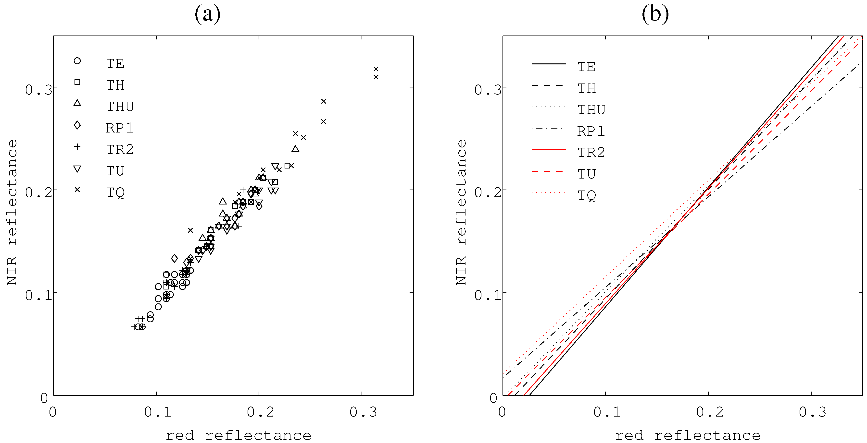
2. Sample Spectra of Bare Soil Pixels and Soil Lines

| Soils*1 | pH | OM*2 | Texture | Fe2O3*3 | CEC*4 | Depth | ||
| Sand | Silt | Clay | ||||||
| TE | 5.2 | 21 | 270 | 180 | 550 | 180 | 78 | >2.0 |
| TH | 3.9 | 21 | 263 | 120 | 617 | 213 | 60 | >2.0 |
| PH | 3.9 | 30 | 320–600 | 500–800 | 300–600 | 80 | 121 | >2.0 |
| RP1 | 4.8–5.2 | 20–24 | 160 | 160 | 680 | 100 | 127 | 1.5–2.0 |
| RP2 | 5.6 | 26 | 290 | 190 | 520 | 120 | 141 | 1.5–2.0 |
| TQ | 3.9 | 12 | 850 | 70 | 80 | 18 | 36 | >2.0 |
| TU | 5.2 | 26 | 200 | 380 | 420 | 70 | 174 | <0.5 |

| a | ||||||||
| TE | 1.16 | –3.00 | 0.89 | 8.2 | 11.1 | 14.1 | 6.7 | 14.1 |
| TH | 1.06 | –1.24 | 0.96 | 11.0 | 16.8 | 22.7 | 10.6 | 22.4 |
| PH | 1.03 | –0.25 | 0.91 | 14.1 | 18.8 | 23.5 | 14.1 | 23.9 |
| RP1 | 0.88 | 1.71 | 0.92 | 11.8 | 15.8 | 20.0 | 12.9 | 19.6 |
| RP2 | 1.12 | –2.29 | 0.96 | 7.8 | 13.1 | 18.4 | 6.7 | 20.0 |
| TU | 1.00 | –0.50 | 0.95 | 12.9 | 17.2 | 21.6 | 12.2 | 22.4 |
| TQ | 0.94 | 2.13 | 0.97 | 13.3 | 25.2 | 37.3 | 13.3 | 36.9 |
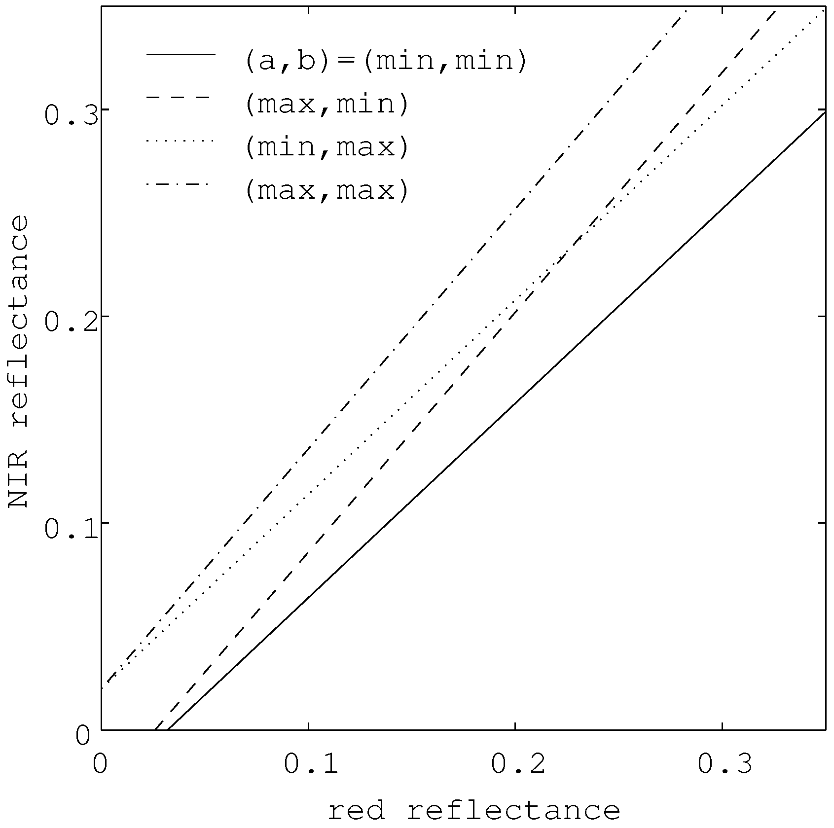
| Initial Values | Variation ranges | ||||
| a | b | ||||
| 1.05 | -0.005 | 0.1, 0.2, 0.3 | –0.03, 0.0, 0.03 | –0.11 ∼ 0.11 | –0.025 ∼ 0.025 |
3. Vegetation Isoline Equations and Numerical Procedures
4. Demonstrations of Soil Line Influences on Vegetation Isolines and VIs
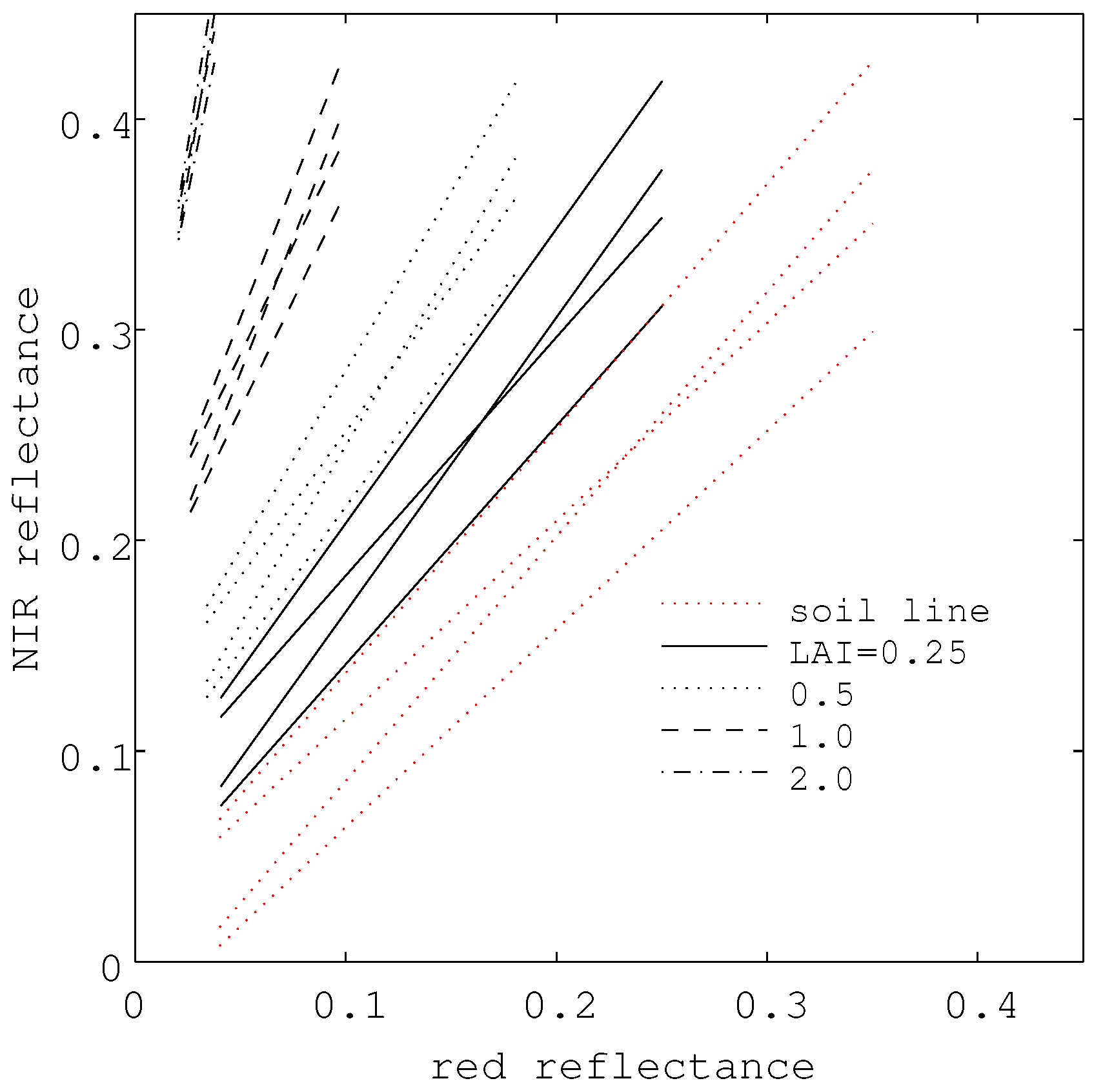
4.1. Variations of Vegetation Isolines

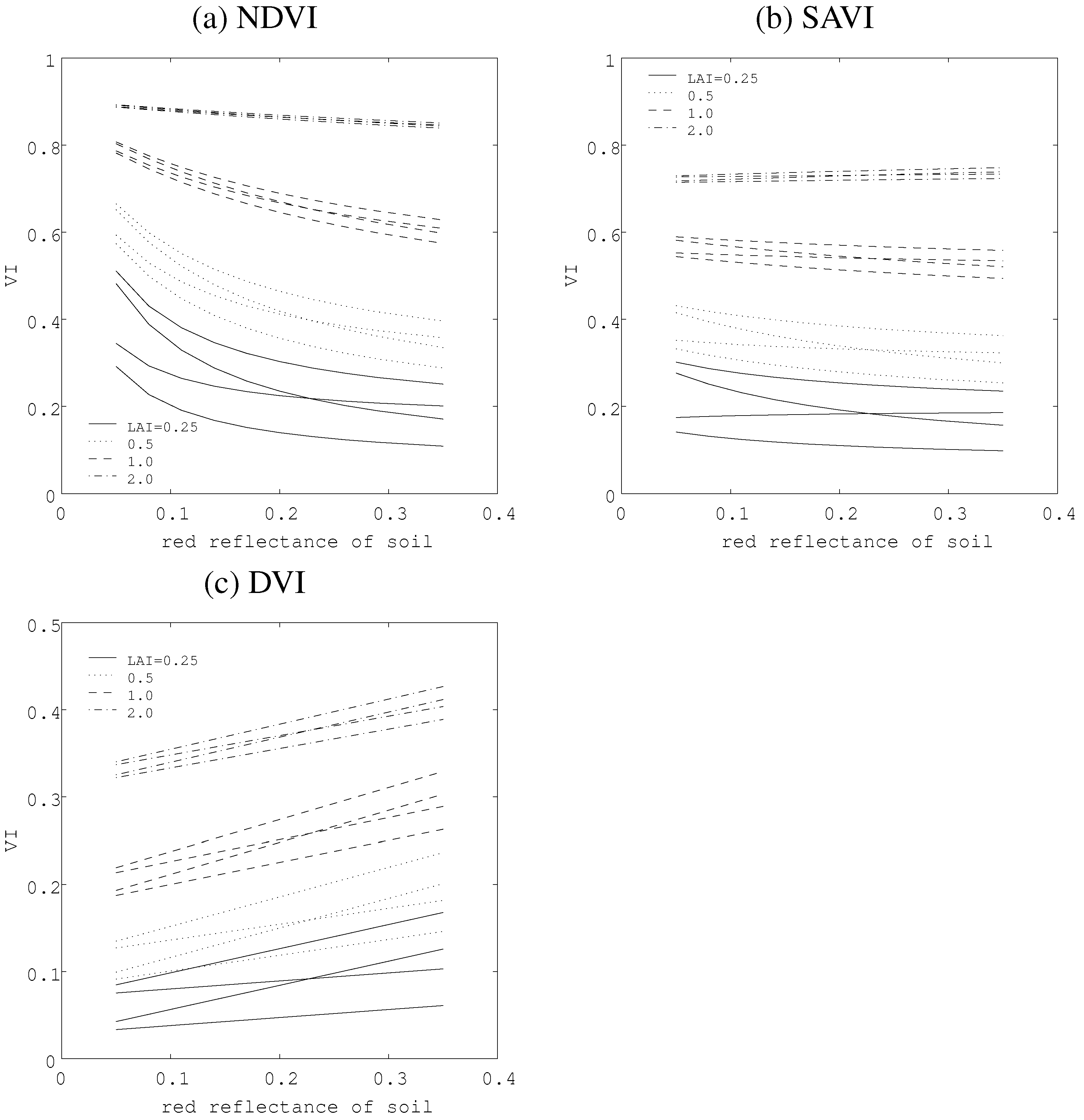
4.2. Variations of VIs
5. Variations of Relative VI Difference ()
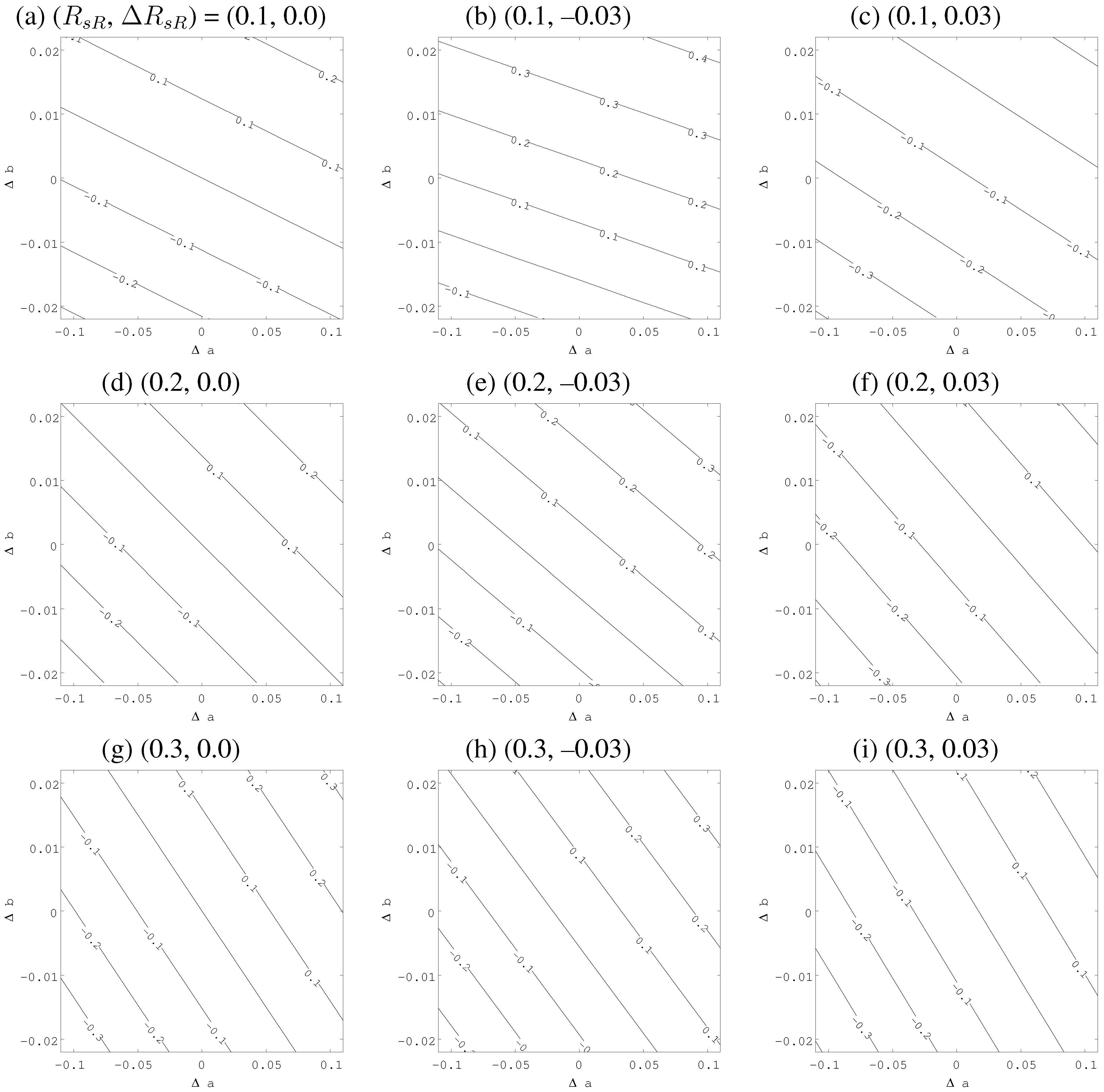
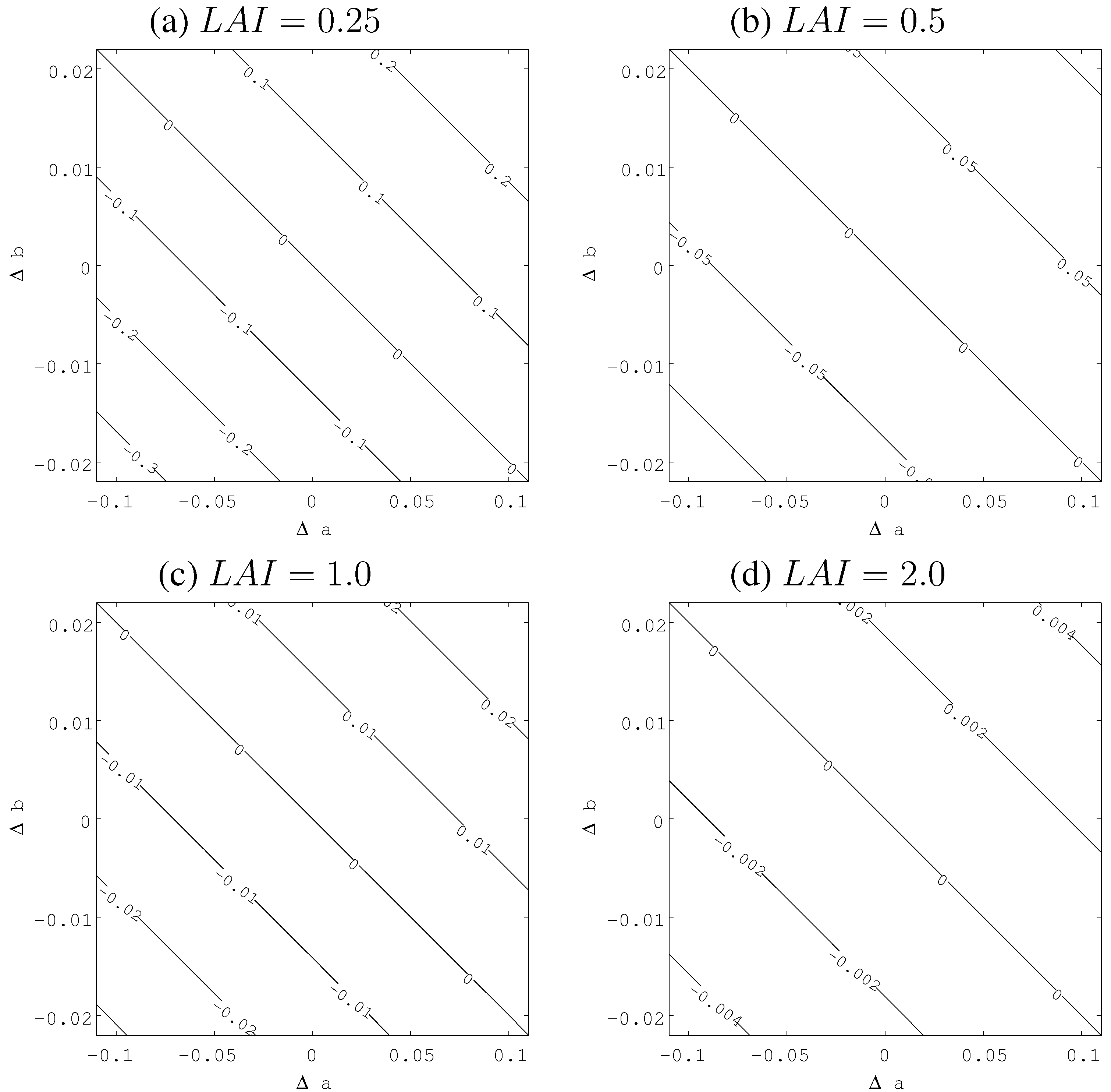
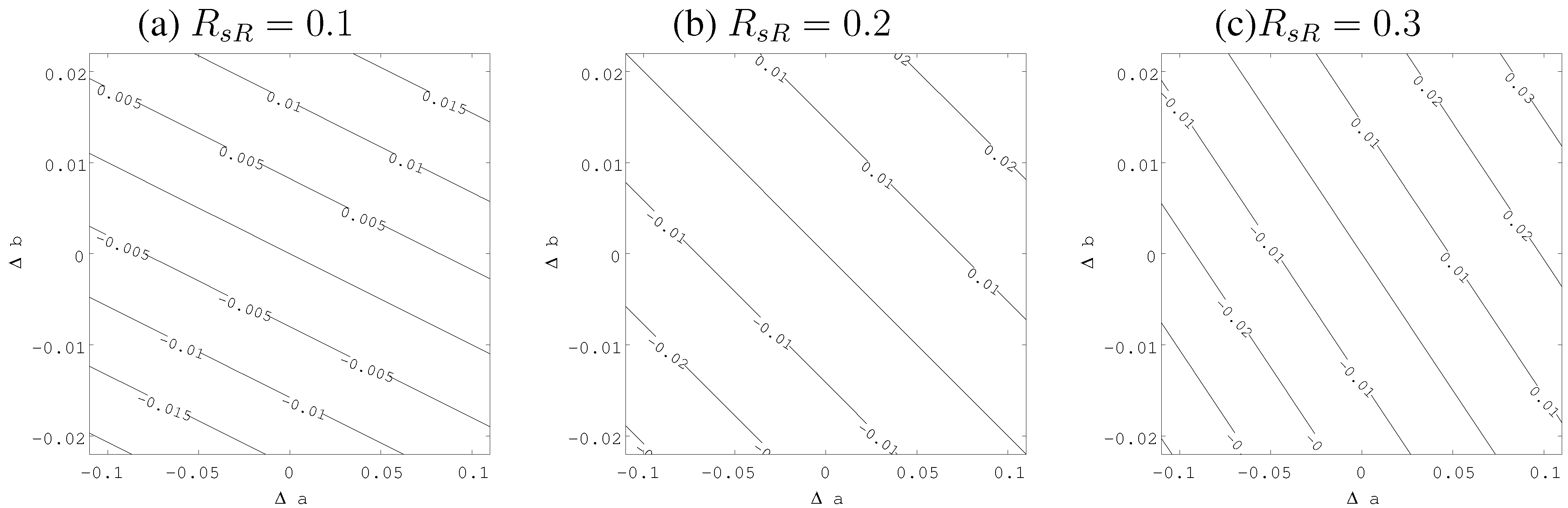
5.1. as a function of , , and
5.2. Variations of
5.3. Iso-Plane of Constant
6. Hypothetical Case Study
| [%] | *1 [%] | |||
| TE | –0.20 | –1.3 | 11.1 | 2.9 |
| TH | –0.30 | 0.5 | 16.8 | 5.9 |
| PH | –0.33 | 1.5 | 18.8 | 4.7 |
| RP1 | –0.48 | 3.4 | 15.8 | 4.1 |
| RP2 | –0.24 | –0.6 | 13.1 | 5.3 |
| TU | –0.36 | 1.2 | 17.2 | 4.3 |
| TQ | –0.42 | 3.8 | 25.2 | 12.0 |
| TE | TH | PH | RP1 | RP2 | TU | TQ | |
| 0.03 | –29.5 / –5.2 *1 | –33.8 / –7.7 | –31.8 / –6.8 | –34.9 / –6.7 | –31.8 / –7.2 | –35.1 / –6.9 | -43.4 / -11.9 |
| 0.0 | –24.4 / –2.2 | –25.7 / –2.9 | –24.8 / –3.0 | –24.1 / –2.6 | –23.8 / –2.3 | –27.9 / –3.2 | –29.6 / –4.2 |
| –0.03 | –16.6 / 1.4 | –10.9 / 3.5 | –14.3 / 1.7 | –8.1 / 2.3 | –7.9 / 4.1 | –16.9 / 1.4 | 1.8 / 7.5 |
7. Remarks
Acknowledgements
References
- Yoshioka, H.; Miura, T.; Demattê, J.A.M.; Batchily, K.; Huete, A.R. Derivation of soil line influence on two-band vegetation indices and vegetation isolines. Remote Sens. 2009, 1, 842–857. [Google Scholar] [CrossRef]
- Baret, F.; Jackquemoud, S.; Hanocq, J.F. About the soil line concept in remote sensing. Remote Sens. Rev. 1993, 5, 281–284. [Google Scholar] [CrossRef]
- Richardson, A.J.; Wiegand, C.L. Distinguishing vegetation from soil background information. Photogramm. Eng. Remote Sens. 1977, 43, 1541–1552. [Google Scholar]
- Baret, F.; Guyot, G. Potentials and limits of vegetation indices for LAI and APAR assessment. Remote Sens. Environ. 1991, 35, 161–173. [Google Scholar] [CrossRef]
- Clevers, J.G.P.W. The application of a weighted infrared-red vegetation index for estimating leaf area index by correcting for soil moisture. Remote Sens. Environ. 1989, 29, 25–37. [Google Scholar] [CrossRef]
- Gilabert, M.A.; González-Piqueras, J.; Garcia-Haro, F.J.; Meliá, J. A generalized soil-adjusted vegetation index. Remote Sens. Environ. 2002, 82, 303–310. [Google Scholar] [CrossRef]
- Huete, A.R.; Jackson, R.D.; Post, D.F. Soil spectral effects on 4-space vegetation discrimination. Remote Sens. Environ. 1984, 15, 155–165. [Google Scholar] [CrossRef]
- Huete, A.R.; Jackson, R.D.; Post, D.F. Spectral response of a plant canopy with different soil backgrounds. Remote Sens. Environ. 1985, 17, 37–54. [Google Scholar] [CrossRef]
- Huete, A.R. Separation of soil plant spectral mixtures by factor analysis. Remote Sens. Environ. 1986, 61, 24–33. [Google Scholar] [CrossRef]
- Huete, A.R. A soil-adjusted vegetation index (SAVI). Remote Sens. Environ. 1988, 25, 295–309. [Google Scholar] [CrossRef]
- Qi, J.; Chehbouni, A.; Huete, A.R.; Kerr, Y.H.; Sorooshian, S. A modified soil adjusted vegetation index. Remote Sens. Environ. 1994, 48, 119–126. [Google Scholar] [CrossRef]
- Rondeaux, G.; Steven, M.; Baret, F. Optimization of soil-adjusted vegetation indices. Remote Sens. Environ. 1996, 55, 95–107. [Google Scholar] [CrossRef]
- Baumgardner, M.F.; Silva, L.F.; Biehe, L.L.; Stoner, E.R. Reflectance properties of soils. Adv. Agron. J. 1985, 38, 1–44. [Google Scholar]
- Fox, G.A.; Sabbagh, G.J. Estimation of soil organic matter from Red and Near-Infrared remotely sensed data using a soil line Euclidean distance technique. Soil Sci. Soc. Am. J. 2002, 66, 1922–1929. [Google Scholar] [CrossRef]
- Fox, G.A.; Sabbagh, G.J.; Searcy, S.W.; Yang, C. An automated soil line identification routine for remotely sensed images. Soil Sci. Soc. Am. J. 2004, 68, 1326–1331. [Google Scholar] [CrossRef]
- Fox, G.A.; Metla, R. Soil property analysis using principal components analysis, soil line, and regression models. Soil Sci. Soc. Am. J. 2005, 69, 1782–1788. [Google Scholar] [CrossRef]
- Henderson, T.L.; Szilagyi, A.; Baumgardner, M.F.; Chen, C.T.; Landgrebe, D.A. Spectral band selection for classification of soil organic matter content. Soil Sci. Soc. Am. J. 1898, 53, 1778–1784. [Google Scholar] [CrossRef]
- Wilcox, C.H.; Frazier, B.E.; Ball, S.T. Relationship between soil organic carbon and Landsat TM data in Eastern Washington. Photogramm. Eng. Remote Sens. 1994, 60, 777–781. [Google Scholar]
- Frazier, B.E. Use of Landsat Thematic Mapper band ratios for soil investigations. Adv. Space Res. 1989, 9, 155–158. [Google Scholar] [CrossRef]
- Jasinski, M.F.; Eagleson, P.S. The structure of red-infrared scattergrams of semivegetated landscapes. IEEE Trans. Geosci. Remote Sens. 1989, 27, 441–451. [Google Scholar] [CrossRef]
- Flenet, F.; Kiniry, J.R.; Board, J.E.; Westgate, M.E.; Reicosky, D.C. Row spacing effects on light extinction coefficients of corn, sorghum, soybean, and sunflower. Agron. J. 1996, 88, 185–190. [Google Scholar] [CrossRef]
- Jordan, C.F. Derivation of leaf area index from quality of light on the forest floor. Ecology 1969, 50, 663–666. [Google Scholar] [CrossRef]
- Tucker, C.J. Red and photographic infrared linear combinations for monitoring vegetation. Remote Sens. Environ. 1979, 8, 127–150. [Google Scholar] [CrossRef]
- Verstraete, M.M.; Pinty, B. Designing optimal spectral indices for remote sensing applications. IEEE Trans. Geosci. Remote Sens. 1996, 34, 1254–1265. [Google Scholar] [CrossRef]
- Galvao, L.S.; Vitorello, I. Variability of laboratory measured soil lines of soils from southeastern Brazil. Remote Sens. Environ. 1998, 63, 166–181. [Google Scholar] [CrossRef]
- Ben-Dor, E.; Irons, J.R.; Epema, G.F. Remote sensing for the earth science. In Manual of Remote Sensing vol.3; Rencz, A.N., Ed.; Wiley: New York, NY, USA, 1999; pp. 111–188. [Google Scholar]
- Elvidge, C.D.; Lyon, R.J.P. Influence of rock-soil spectral variation on the assessment of green biomass. Remote Sens. Environ. 1985, 17, 265–269. [Google Scholar] [CrossRef]
- Huete, A.R. Soil influences in remotely sensed vegetation-canopy spectra. In Theory and Applications of Optical Remote Sensing; Asrar, G., Ed.; Wiley: New York, NY, USA, 1989; pp. 107–141. [Google Scholar]
- Nanni, M.R.; Demattê, J.A.M. Spectral reflectance methodology in comparison to traditional soil analysis. Soil Science Soc. Am. J. 2006, 70, 393–407. [Google Scholar] [CrossRef]
- Valeriano, M.M.; Epiphanio, J.C.N.; Formaggio, A.R.; Oliveira, J.B. Bidirectional reflectance factor of 14 soil classes from Brazil. Int. J. Remote Sens. 1995, 16, 113–128. [Google Scholar] [CrossRef]
- Elvidge, C.D.; Chen, Z. Comparison of broad-band and narrow-band red and near-infrared vegetation indices. Remote Sens. Environ. 1995, 51, 38–48. [Google Scholar] [CrossRef]
- Gitelson, A.A.; Kaufman, Y.J. MODIS NDVI optimization to fit the AVHRR data series-spectral considerations. Remote Sens. Environ. 1998, 66, 343–350. [Google Scholar] [CrossRef]
- Gobron, N.; Pinty, B.; Verstraete, M.M.; Widlowski, J. Advanced vegetation indices optimized for up-coming sensors: design, performance, and applications. IEEE Trans. Geosci. Remote Sens. 2000, 38, 2489–2505. [Google Scholar]
- Huete, A.R.; Tucker, C.J. Investigation of soil influences in AVHRR red and near-infrared vegetation index imagery. Int. J. Remote Sens. 1991, 12, 1223–1242. [Google Scholar] [CrossRef]
- Major, D.J.; Baret, F.; Guyot, G. A ratio vegetation index adjusted for soil brightness. Int. J. Remote Sens. 1990, 115, 727–40. [Google Scholar] [CrossRef]
- Pinty, B.; Verstraete, M.M. GEMI: a non-linear index to monitor global vegetation from satellites. Vegetatio 1992, 101, 15–20. [Google Scholar] [CrossRef]
- Yoshioka, H.; Huete, A.R.; Miura, T. Derivation of vegetation isoline equations in red-NIR reflectance space. IEEE Trans. Geosci. Remote. Sens. 2000, 38, 838–848. [Google Scholar] [CrossRef]
- Yoshioka, H.; Miura, T.; Huete, A.R.; Ganapol, B.D. Analyses of vegetation isoline equations in red-NIR reflectance space. Remote Sens. Environ. 2000, 74, 313–326. [Google Scholar] [CrossRef]
- Demattê, J.A.M.; Huete, A.R.; Guimaraes, L.; Nanni, M.R.; Alves, M.C.; Fiorio, P.R. Methodorogy for bare soil detection and discrimination by Landsat-TM image. The Open Remote Sens. 2009, 2, 24–35. [Google Scholar] [CrossRef]
- Demattê, J.A.M.; Huete, A.R.; Ferreira, L.G., Jr.; Alves, M.C.; Nanni, M.R.; Cerri, C.E. Evaluation of tropical soils through ground and orbital sensors. In Proceedings of the Second International Conference Geospatial Information in Agriculture and Forestry, Lake Buena Vista, FL, USA, 2000; pp. 34–41.
- Epiphanio, J.C.N.; Formaggio, A.R.; Valeriano, M.M.; Oliveira, J.B. The spectral behavior of soils from the Sao Paulo state. In INPE Tech. Rep. 5424; Institute Nacional de Pesquisas Espaciais: Sao Jose dos Campos, SP, Brasil, 1992. (In Portuguese) [Google Scholar]
- Formaggio, A.R.; Epiphanio, J.C.N.; Valeriano, M.M. Spectral behavior (450–2450 nm) of tropical soils from Sao Paulo State, Brazil. Braz. J. Soil Sci. 1996, 20, 467–474. (In Portuguese) [Google Scholar]
- Soil Survey Staff. Key to Soil Taxonomy, 8th edUSDA Soil Conservation Service: Washington, DC, USA, 1998.
- Vermote, E.; Tanre, D.; Herman, M.; Morcrette, J.J. Second simuation of the satellite signal in the solar spectrum (6S). In 6S User Guide Version 1; LOA-USTL: Villeneuve d’Ascq, France, 1997; p. 216. [Google Scholar]
- Clevers, J.G.P.W. The derivation of a simplified reflectance model for the estimation of leaf area index. Remote Sens. Environ. 1988, 25, 53–69. [Google Scholar] [CrossRef]
- Verhoef, W. Light scattering by leaf layers with application to canopy reflectance modeling: the SAIL model. Remote Sens. Environ. 1984, 16, 125–141. [Google Scholar] [CrossRef]
- Verhoef, W. Earth observation modeling based on layer scattering matrices. Remote Sens. Environ. 1985, 17, 165–178. [Google Scholar] [CrossRef]
© 2010 by the authors; licensee Molecular Diversity Preservation International, Basel, Switzerland. This article is an open-access article distributed under the terms and conditions of the Creative Commons Attribution license http://creativecommons.org/licenses/by/3.0/.
Share and Cite
Yoshioka, H.; Miura, T.; Demattê, J.A.M.; Batchily, K.; Huete, A.R. Soil Line Influences on Two-Band Vegetation Indices and Vegetation Isolines: A Numerical Study. Remote Sens. 2010, 2, 545-561. https://doi.org/10.3390/rs2020545
Yoshioka H, Miura T, Demattê JAM, Batchily K, Huete AR. Soil Line Influences on Two-Band Vegetation Indices and Vegetation Isolines: A Numerical Study. Remote Sensing. 2010; 2(2):545-561. https://doi.org/10.3390/rs2020545
Chicago/Turabian StyleYoshioka, Hiroki, Tomoaki Miura, José A. M. Demattê, Karim Batchily, and Alfredo R. Huete. 2010. "Soil Line Influences on Two-Band Vegetation Indices and Vegetation Isolines: A Numerical Study" Remote Sensing 2, no. 2: 545-561. https://doi.org/10.3390/rs2020545