Land-Cover Phenologies and Their Relation to Climatic Variables in an Anthropogenically Impacted Mediterranean Coastal Area

Abstract

Mediterranean coastal areas are experiencing rapid land cover change caused by human-induced land degradation and extreme climatic events. Vegetation index time series provide a useful way to monitor vegetation phenological variations. This study quantitatively describes Enhanced Vegetation Index (EVI) temporal changes for Mediterranean land-covers from the perspective of vegetation phenology and its relation with climate. A time series from 2001 to 2007 of the MODIS Enhanced Vegetation Index 16-day composite (MOD13Q1) was analyzed to extract anomalies (by calculating z-scores) and frequency domain components (by the Fourier Transform). Vegetation phenology analyses were developed for diverse land-covers for an area in south Alicante (Spain) providing a useful way to analyze and understand the phenology associated to those land-covers. Time series of climatic variables were also analyzed through anomaly detection techniques and the Fourier Transform. Correlations between EVI time series and climatic variables were computed. Temperature, rainfall and radiation were significantly correlated with almost all land-cover classes for the harmonic analysis amplitude term. However, vegetation phenology was not correlated with climatic variables for the harmonic analysis phase term suggesting a delay between climatic variations and vegetation response.

1. Introduction

Human activities can generate severe negative impacts in the Earth system, resulting in environmental changes greater than natural variability [1]. The term Global Change is commonly employed to refer to such environmental changes. This concept considers a wide range of changes in Earth ecosystems with three common characteristics: (1) changes of human origin; (2) an exponential growth rate over time; and (3) a global scale manifestation [2]. Factors such as habitat change, overexploitation of natural resources, invasive species introduction, pollution and climate change have been recognized as major global change drivers [3]. Land-cover (i.e., biophysical attributes of the Earth’s surface) and land-use (human purpose applied to these attributes) changes are among the most important drivers of the Earth’s global change [4,5], and significantly affect key aspects of Earth System functioning [6]. In fact, land-use/land-cover changes have been identified as the factor with the largest effect on terrestrial ecosystems than any other driver of global change [7].

Land-cover changes may result from human-induced land-use changes or natural processes such as climatic variability and natural disturbances [8]. The status and rate of land-cover changes may be estimated through a monitoring approach with remotely sensed data [9]. Thus, Earth-observing systems allow the study of the role of terrestrial vegetation in large-scale global processes (e.g., the carbon cycle) with the goal of understanding how the Earth functions as a system [10]. In fact, satellite data provides a synoptic view, worldwide coverage and repeated temporal sampling of the Earth’s surface with a great potential for monitoring vegetation dynamics from regional to global scales [11]. Accurate, timely information on the distribution of vegetation on the Earth's surface is a pre-requisite for understanding how changes in land-cover affect phenomena as diverse as atmospheric CO₂ concentrations, terrestrial primary productivity, the hydrologic cycle, and the energy balance at the surface-atmosphere interface [12].

Vegetation indices have been used to derive a measure that correlates with surface biophysical properties [13] that facilitate the analysis of large amounts of satellite data, thereby providing valuable large spatial- and temporal-scale analyses [12]. The fact that vegetation indices are directly related to plant vigor, density, and growth conditions, means that they can be used to detect environmental conditions like droughts in semiarid regions [9]. During the last decades, multiple studies have provided a wide range of vegetation indices, the most frequently used being the Normalised Difference Vegetation Index (NDVI) described by Rousse et al. [14]. Despite the undeniable usefulness of the NDVI, it has some constraints inherent to vegetated canopies (i.e., canopy background contamination and saturation problems) which restrict its use and interpretation [15]. In this sense, many indices have been developed to minimize these limitations. The Enhanced Vegetation Index (EVI) described by Huete et al. [15] was employed in this study. This index has been implemented as a standard product (along with NDVI) for the data acquired by the Moderate Resolution Imaging Spectroradiometer (MODIS) sensor. A MODIS-EVI dataset was used for the selected study area.

Vegetation indices have contributed to characterize seasonal variations and phenologic activity of vegetation in time series of satellite data, providing baseline data to monitor length of the growing season, peak greenness, onset of greenness, or land-cover changes associated with events such as fire, drought, land-use conversion, and climate fluctuation [15,16,17]. The study of vegetation-index time series for the analyses of vegetation phenology is highly complex and multiple approaches and techniques have been developed. Time series anomalies and the Fourier Transform (FT) are commonly used techniques for vegetation phenology analyses. Vegetation index time series anomalies, defined as differences between standardized EVI values from their mean-daily (or any other unit of time) values attempt to track daily values (or the corresponding unit of time) that are associate to the degree of wetness or dryness (positive or negative anomaly values) of the condition of ground vegetation [18]. On the other hand, the application of the Fourier Transform (harmonic analysis) facilitates the extraction of valuable and interpretable characteristics from the time series, which are usually disturbed by atmospheric noise, sensor instability or orbit deviations [19]. Harmonic analysis of remote sensing time-series can be used to detect changes in land use/land covers by examining changes in annual values of amplitude, phase, or the additive term over a period of years [20]. In addition, the amplitude and phase values of the harmonic terms for the different frequencies inform about the relative importance of periodic climate processes [21]. Harmonic analysis of time-series data offers a valuable tool for monitoring land surface phenologies [16,22], for mapping land-uses [20,23], for modeling bioclimatic indices [24], or monitoring flooding extent [25].

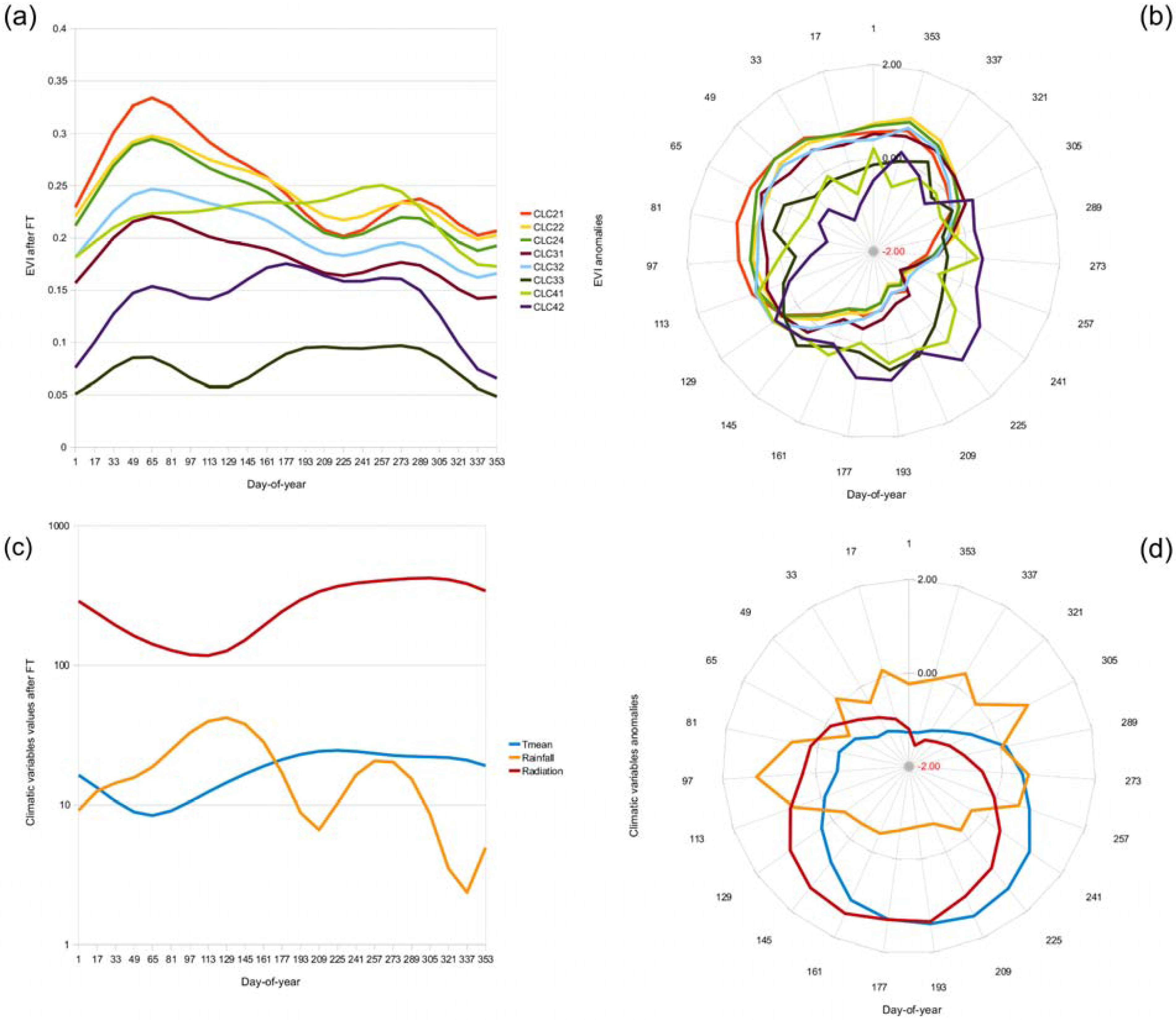
This study quantitatively describes EVI temporal changes for Mediterranean land-covers from the viewpoint of vegetation phenology and its relation with climate. MODIS-EVI time series anomalies and Fourier Transform parameters provided valuable information about the dynamics of vegetation during the period 2001–2007. Time series of climatic variables were analyzed in the same way that the time series of the vegetation index. Significant correlations between vegetation and climate time series parameters were searched for to better understand the response of vegetation land-covers to climate variability.

2. Material and Methods

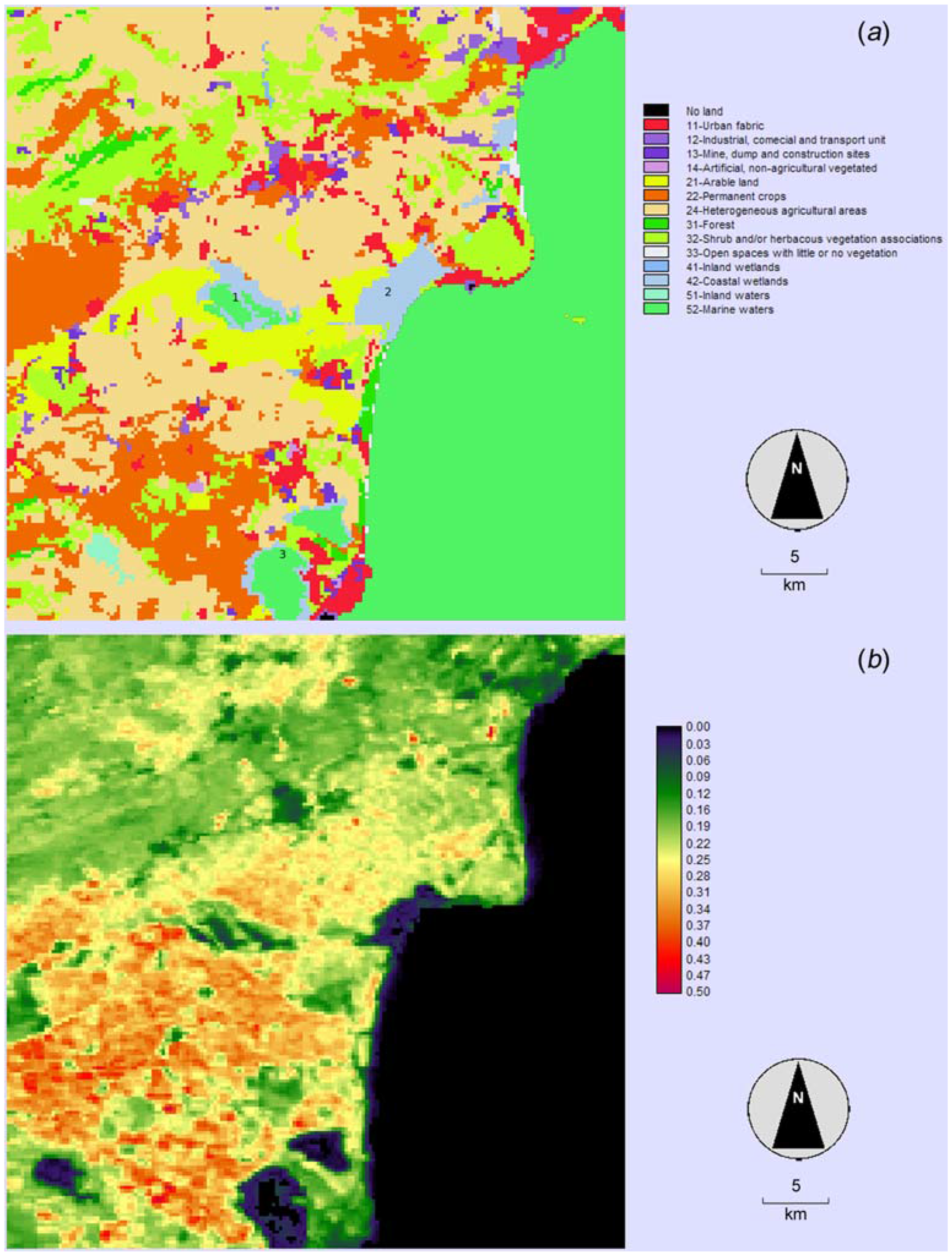
The study area is located in a coastal zone of SE Spain in southern Alicante province. It is located around 38.18°N latitude and 0.68°W longitude. The study area is 45 × 45 kilometers in area, accounting for a total of 2,025 square kilometers. This area is a mixture of medium size cities, coastal urban areas, scattered residential houses, irrigated crops and isolated and scattered wetlands. The climate of the study area is defined by the Köppen climate classification system as Bsk class (dry climate with a dry season in summer and a mean annual temperature of less than 18 ºC). The climate is arid or semiarid according to the aridity index of Martonne [26] and the aridity index of UNEP [27] respectively. Major soil groups in the study area include Fluvisols, Calcisols, Solonchaks and Gleysols [28,29] based on the World Reference Base for Soil Resources [30].

Vegetation phenology was assessed by analyzing time series anomalies of vegetation index and Fourier Transform parameters for a 16-day time series from 2001 to 2007. The selected vegetation index was the EVI acquired by the moderate resolution MODIS sensor at 16-day time interval, a standard product coded as MOD13Q1. A total of 161 EVI 16-day composite images were employed in the analyses. Land cover information was obtained from the CORINE Land-cover (CLC) 2000 database of the European Environmental Agency. This database provided information about the European Union land-cover for the year 2000. CLC cartography uses a hierarchical system of land-cover classes with different levels of specificity. This analysis employed a Level II coverage that provided a good description of land-cover for the study area. Table 1 shows land-cover identified for the study area and their surfaces (percentage of terrestrial area). EVI time series phenology analyses were carried out for all land-cover classes with the exception of urban-industrial areas (CLC11 to CLC14) and water bodies (CLC51 and CLC52) because of by their low or null-vegetation presence. A stratified random sampling (stratification based on the land-cover map) was performed on the images of the EVI time series. About 1,500 pixels were selected after visual inspection in order to avoid outliers and pixels that have undergone land-use changes during the study period. These pixels were used to extract the values of EVI from each image of the time series. A final matrix with 161 EVI values and land-cover classes for each pixel was obtained and employed for the vegetation analyses.

Table 1. CORINE land-cover 2000 level II land-cover classes of the study area, and their relative areas.

Code	Land-covers	Surface coverage (%)
CLC11	Urban	6.93
CLC12	Industrial, commercial and transport unit	1.79
CLC13	Mine, dump and construction sites	1.28
CLC14	Artificial, non-agricultural vegetated	0.30
CLC21	Arable land	6.43
CLC22	Permanent crops	19.96
CLC24	Heterogeneous agricultural areas	39.29
CLC31	Forest	1.52
CLC32	Shrub and/or herbaceous vegetation associations	16.17
CLC33	Open spaces with little or no vegetation	0.33
CLC41	Inland wetlands	0.15
CLC42	Coastal wetlands	3.34
CLC51	Inland water	0.39
CLC52	Marine waters	2.13

Table 1. CORINE land-cover 2000 level II land-cover classes of the study area, and their relative areas.

Code	Land-covers	Surface coverage (%)
CLC11	Urban	6.93
CLC12	Industrial, commercial and transport unit	1.79
CLC13	Mine, dump and construction sites	1.28
CLC14	Artificial, non-agricultural vegetated	0.30
CLC21	Arable land	6.43
CLC22	Permanent crops	19.96
CLC24	Heterogeneous agricultural areas	39.29
CLC31	Forest	1.52
CLC32	Shrub and/or herbaceous vegetation associations	16.17
CLC33	Open spaces with little or no vegetation	0.33
CLC41	Inland wetlands	0.15
CLC42	Coastal wetlands	3.34
CLC51	Inland water	0.39
CLC52	Marine waters	2.13

Several daily climatic variables, namely mean temperature (Tmean, °C), maximum temperature (Tmax, °C), minimum temperature (Tmin, °C), rainfall (mm), incoming solar radiation (MJ m⁻² day⁻¹) and evapotranspiration (ETP, mm), were used as explanatory variables for the discussion of the vegetation phenology behavior. Climatic variables were obtained from five meteorological stations maintained by the Spanish Ministry of Environment (MARM). Meteorological stations are located in a coastal plain with low climate variability. Therefore, they can be assumed to be representative of the climatic conditions of the study area. For each meteorological station, daily values of climatic variables were computed (i.e., average temperatures, and accumulated rainfall, radiation and ETP) for the same 16-day time intervals of EVI time series.

A brief description of the vegetation index time series, the time series anomaly analysis method, the Fourier Transform method and the statistical methods to assess the relationship between vegetation phenology and climatic variables are presented.

2.1. MODIS-EVI Time Serie

EVI is a vegetation index optimized to avoid background and atmospheric influences [15]. EVI is based in the approach developed by Liu and Huete [31] to incorporate both background adjustment and atmospheric resistance concepts and thus improve on the Normalised Difference Vegetation Index (NDVI) which was originally developed by Rouse et al. [14]. This resulted in the enhanced soil and atmosphere resistant-vegetation index (EVI) adopting the following expression [15]:

$$EVI=\frac{\left({\rho }_{NIR}-{\rho }_R\right)}{\left(L+{\rho }_{NIR}+C_1\cdot {\rho }_R+C_2\cdot {\rho }_B\right)}$$

(1)

where ρ_NIR, ρ_R, ρ_B are ‘apparent’ (top-of-the-atmosphere) or ‘surface’ directional reflectance for the NIR (near infrared), red and blue bands respectively. L is a canopy background adjustment term, and C₁ and C₂ weight the use of the blue channel in aerosol correction of the red channel.

A time series of satellite images acquired by the TERRA-MODIS sensor was used for the analysis. The selected MODIS product was an EVI thematic product, namely MOD13Q1 Version 005. MOD13Q1 is a Level II product that contains EVI 16-day composites at 250 m spatial resolution image data acquired by the Terra satellite. An EVI time series from 2001 to 2007 composed of 161 MOD13Q1 images was analyzed.

MODIS data were transformed from Sinusoidal projection to UTM projection for a subset of 45 × 45 km over the study area. MODIS time series were geometrically co-registered to a Landsat ETM+ scene from 8 July 2001 (with 30 m of spatial resolution). Landsat ETM+ scene had been previously geometrically corrected using aerial orthophotography and vector cartography at a scale of 1:10,000.

2.2. Detection and Quantification of Time Series Anomalies

The analysis of vegetation index time series anomalies is a useful method of assessing the degree of wetness or dryness of the condition of ground vegetation for each time unit in relation to the average value of the time series [18]. Time series anomalies were computed for each 16-day EVI composite value in relation to the average EVI value from 2001 to 2007. The time series anomaly was computed using the following expression:

$$T{S}_{anomaly}=\frac{T{S}_t-T{S}_{\Delta t}}{{\sigma }_{\Delta t}}$$

(2)

where TS_t is the time series value for a given moment, and TS_Δt and σ_Δt are respectively the mean value and the standard deviation value of the time series for the full period of time studied. When the TS_anomaly is negative, it indicates below-normal vegetation conditions, thereby pointing to prevailing drought, and when it is positive it indicates above normal vegetation conditions thereby pointing to wetness [18]. Time series anomalies of the climatic variables were also computed. Time series anomalies have been previously employed for vegetation index time series analysis in relation to climatic variables [32,33]. It provided an intuitive way to identify intensity and duration of the canopy change/stress or different climatic variations.

Various non-dimensional coefficients have been previously described to represent magnitude and timing of the anomalies of a time series, such as [33]: (1) coefficient D, that is the sum of negative anomalies for a given study period; and (2) coefficient S, that is the sum of positive anomalies for a given study period. Both coefficients were computed for time series of EVI and climatic variables for each year of the studied period. Finally, a new coefficient that we named normalized D/S was computed as a normalized coefficient between coefficient D and coefficient S. The normalized D/S coefficient synthesized in a single value the general pattern of time series anomalies for each year. Values range between −1 to +1. For the EVI time series, negative normalized D/S coefficient values represent a year above normal vegetation (or climatic variable) conditions, while a positive value represent a year below normal vegetation (or climatic variable) conditions.

2.3. Fourier Transform

MODIS-EVI time series were analyzed by the Fourier Transform to obtain its frequency domain components. Fourier analysis allows the decomposition of temporal data to the frequency domain, by which frequency information is represented in terms of the sum of a set of sine and cosine functions [34]. Harmonic or Fourier analysis allows a complex curve to be expressed as the sum of a cosine waves (terms) and an additive term [35,36]. The Fourier Transform converts a function f(x) to the frequency domain by a linear combination of trigonometric functions as follows [22]:

$$F(\omega )={\displaystyle \underset{-\infty }{\overset{+\infty }{\int }}f(x)e^{-i\omega x}}dx$$

(3)

where ω is the frequency and F(ω) is the Fourier coefficient with frequency ω. It is customary to use a discrete form as follows [22]:

$$F(k)=\frac{\text{1}}{N}{\displaystyle \sum _{n=\text{0}}^{N-\text{1}}{f}_i{e}^{\left(-\frac{\text{2π}kni}{N}\right)}}$$

(4)

where K = 0, 1, 2, …, N–1 and N is the total number of input data.

For a correct interpretation of harmonic analysis results, several key-concepts must be considered [37]: (1) each wave is defined by a unique amplitude and phase angle, where amplitude is the difference between the maximum value of a wave and the overall average of the time series (usually 0 because the mean is equal to the harmonic term with k = 0), and the phase angle defines the offset between the origin and the peak of the wave over the range 0 to 2π; (2) the additive or zero term is the arithmetic mean of the variable over the time series; (3) high amplitude values for a given term indicate a high level of variation in temporal variable time series, and the term in which that variation occurs indicate the periodicity of the event; and (4) phase indicates the time of year at which the peak value for a term occurs. Each term indicates the number of complete cycles completed by a wave over a defined interval [20]. The Fourier Transform was applied individually for each studied year. The additive term and the first three harmonic components for each year of the EVI time series were extracted for all land-cover classes for subsequent analysis. IDRISI Andes © software was employed for the harmonic analysis of the time series.

2.4. Statistical Analysis

Statistical analyses were used to assess different phenological responses of vegetation, and to determine the influence of climatic variables on those vegetation land-covers.

Annual EVI differences for selected land-cover were assessed with the one-way Analysis of Variance (ANOVA) test using years as factor. Pairwise comparisons were performed with the Tukey post-hoc test at the P < 0.05 significance level. Homogeneous subgroups (years with similar EVI values) were defined based on the post-hoc test results.

A two-way ANOVA test was employed to assess annual differences and differences among meteorological stations for the climatic variables time series. Climatic variables with significant differences among meteorological stations were discarded for further analysis because such variables did not show a homogeneous spatial pattern.

Pearson bivariate correlations were used to analyze the influence of climatic variables on location-specific land-cover phenology. Pearson correlation coefficients were computed by using as variables several parameters such as: the anomaly values for the full time series (ATS), the normalized D/S values for each year (NDS), annual amplitude (for the first three harmonic terms and the additive one) values computed with the Fourier Transform (FT-A), and annual phase (for the first three harmonic terms) values computed with the Fourier Transform (FT-P).

3. Results and Discussion

3.1. Land-Covers and Average EVI for the Study Area

A general overview of the spatial distribution of land-cover in the study area was obtained with the CORINE land-cover cartography (Figure 1a and Table 1). Artificial land-covers (CLC11 to CLC14) are concentrated along the coast line or sparsely distributed in the agriculture areas, mainly from the city of Elche to the south of the Alicante province, and occupy a 10.3% of the surface. Agricultural areas (CLC21 to CLC24) dominate the landscape (65.68% of the land surface) with a large proliferation of heterogeneous agricultural areas (39.29% of the land surface). Land-cover (CLC24) was the dominant, corresponding to irrigated agriculture fields of the Camp d’Elx and Vega Baja areas. This class is a mixture of small buildings (farms and rural households) and small-medium size (average area about 1–10 ha) irrigated agriculture fields. Mountainous and low-productivity lands were occupied by forest and semi-natural vegetation areas (CLC31 to CLC33). Several wetlands (CLC41 and CLC42) were located along the coast line and in the middle of the major agricultural area. Three of the wetlands within the study area (i.e., the Natural Park of El Hondo, the Natural Park of Salinas de Santa Pola, and the Natural Park of Salinas de la Mata-Torrevieja) are included in the RAMSAR Convention list for wetlands of international importance (www.ramsar.org). These wetlands act like wildlife reservoirs and are subject to human water-management practices. The Natural Park of El Hondo is a very important water reservoir for surrounding agricultural areas but its water management is often very complex. Previous studies [38] suggest different water management practices within and outside the Park during the drought and different vegetation responses to rainfall patterns can be expected. Figure 1b shows average EVI values for the studied period. Urban areas, large inland water bodies and the sea were masked out to improve the visual analysis of EVI results and for further analysis due to their lack of vegetation (low or null vegetation coverage). Irrigated agriculture areas of the Camp d’Elx and Vega Baja regions had the highest mean EVI values (>0.3), wetlands had mean EVI values close to 0.25, while forest and semi-natural vegetation areas reported at sensibly lower EVI values (~0.2).

Figure 1. Regional analysis maps composition of: (a) CORINE Land Cover Level II land-covers map of the study area; (b) average EVI values for the studied period. Numbers in the land-use map correspond with: (1) the Natural Park of El Hondo; (2) the Natural Park of Salinas de Santa Pola; and (3) the Natural Park of Salinas de la Mata-Torrevieja.

Figure 1. Regional analysis maps composition of: (a) CORINE Land Cover Level II land-covers map of the study area; (b) average EVI values for the studied period. Numbers in the land-use map correspond with: (1) the Natural Park of El Hondo; (2) the Natural Park of Salinas de Santa Pola; and (3) the Natural Park of Salinas de la Mata-Torrevieja.

3.2. Overview of EVI and Climatic Variables Time Series

Annual average values (± standard deviation) of EVI for the eight tested CORINE land-covers were obtained (Table 2). As a general rule, agricultural areas (CLC21, CLC22 and CLC24) have annual EVI values ranging between 0.22 and 0.27. These values are the highest for the study area (agriculture is maintained by irrigation in this semi-arid area) but turns out to be not very high because the pixel size is too big (250 m) to contain only an agricultural plot. There is a mixture of covers within the sensor's instantaneous field of view (IFOW) generating a mixed pixel [39] with an average EVI value. This phenomenon occurs in all land-covers of the study area. P-values of the last row of Table 2 were obtained by the one-way analysis of variance (ANOVA) test and indicate the existence (or not) of significant differences in EVI values between years. Only significant differences (at the 95% confidence level) were observed for the CLC21 land-cover class (P = 0.01) suggesting a temporal variability of average annual EVI values.

Table 2. Mean (± a standard deviation) annual EVI for 2001 to 2007 of selected CORINE land-covers. P-values result from the one-way ANOVA of EVI time series using years as factor. Lower case letters indicate differences between years and homogeneous subgroups (ANOVA, Tukey test, P < 0.05).

Years	CLC21	CLC22	CLC24	CLC31	CLC32	CLC33	CLC41	CLC42
2001	0.26 ± 0.04a	0.25 ± 0.03a	0.24 ± 0.03ab	0.20 ± 0.03c	0.20 ± 0.02a	0.14 ± 0.02b	0.19 ± 0.02a	0.13 ± 0.01ab
2002	0.26 ± 0.04a	0.25 ± 0.03a	0.24 ± 0.03ab	0.18 ± 0.02abc	0.21 ± 0.02ab	0.08 ± 0.03a	0.22 ± 0.02b	0.13 ± 0.02b
2003	0.24 ± 0.03a	0.24 ± 0.02a	0.23 ± 0.03ab	0.18 ± 0.02ab	0.19 ± 0.02a	0.07 ± 0.03a	0.22 ± 0.03b	0.12 ± 0.02ab
2004	0.26 ± 0.04a	0.25 ± 0.03a	0.24 ± 0.03ab	0.18 ± 0.02ab	0.21 ± 0.03ab	0.07 ± 0.03a	0.23 ± 0.03b	0.13 ± 0.01b
2005	0.24 ± 0.03a	0.24 ± 0.02a	0.22 ± 0.02a	0.16 ± 0.02a	0.19 ± 0.02a	0.06 ± 0.02a	0.22 ± 0.02b	0.12 ± 0.01a
2006	0.24 ± 0.04a	0.23 ± 0.02a	0.23 ± 0.03ab	0.16 ± 0.02a	0.20 ± 0.03a	0.06 ± 0.02a	0.23 ± 0.03b	0.12 ± 0.01a
2007	0.27 ± 0.04a	0.25 ± 0.03a	0.25 ± 0.03b	0.20 ± 0.02bc	0.22 ± 0.03b	0.07 ± 0.02a	0.24 ± 0.02b	0.13 ± 0.01b
P-values	0.01	0.037	0.070	<0.001	<0.001	<0.001	<0.001	<0.001

Table 2. Mean (± a standard deviation) annual EVI for 2001 to 2007 of selected CORINE land-covers. P-values result from the one-way ANOVA of EVI time series using years as factor. Lower case letters indicate differences between years and homogeneous subgroups (ANOVA, Tukey test, P < 0.05).

Years	CLC21	CLC22	CLC24	CLC31	CLC32	CLC33	CLC41	CLC42
2001	0.26 ± 0.04a	0.25 ± 0.03a	0.24 ± 0.03ab	0.20 ± 0.03c	0.20 ± 0.02a	0.14 ± 0.02b	0.19 ± 0.02a	0.13 ± 0.01ab
2002	0.26 ± 0.04a	0.25 ± 0.03a	0.24 ± 0.03ab	0.18 ± 0.02abc	0.21 ± 0.02ab	0.08 ± 0.03a	0.22 ± 0.02b	0.13 ± 0.02b
2003	0.24 ± 0.03a	0.24 ± 0.02a	0.23 ± 0.03ab	0.18 ± 0.02ab	0.19 ± 0.02a	0.07 ± 0.03a	0.22 ± 0.03b	0.12 ± 0.02ab
2004	0.26 ± 0.04a	0.25 ± 0.03a	0.24 ± 0.03ab	0.18 ± 0.02ab	0.21 ± 0.03ab	0.07 ± 0.03a	0.23 ± 0.03b	0.13 ± 0.01b
2005	0.24 ± 0.03a	0.24 ± 0.02a	0.22 ± 0.02a	0.16 ± 0.02a	0.19 ± 0.02a	0.06 ± 0.02a	0.22 ± 0.02b	0.12 ± 0.01a
2006	0.24 ± 0.04a	0.23 ± 0.02a	0.23 ± 0.03ab	0.16 ± 0.02a	0.20 ± 0.03a	0.06 ± 0.02a	0.23 ± 0.03b	0.12 ± 0.01a
2007	0.27 ± 0.04a	0.25 ± 0.03a	0.25 ± 0.03b	0.20 ± 0.02bc	0.22 ± 0.03b	0.07 ± 0.02a	0.24 ± 0.02b	0.13 ± 0.01b
P-values	0.01	0.037	0.070	<0.001	<0.001	<0.001	<0.001	<0.001

The lower case letters of Table 2 were employed to mark homogeneous subgroups of years with similar EVI values. These subgroups were based on the post-hoc Tukey test with P < 0.05. No subgroups were identified for CLC21 and CLC22 land-covers. Two subgroups were identified for CLC24 class. A first group of low EVI values (a) and another group of high EVI values (b). The 2005 year had the lowest EVI values and was not included in the b subgroup, while the 2007 year had the highest EVI values and was excluded from the lower EVI values subgroup. This observation suggests that, for the CLC24 class, 2005 was the driest year (and thus lower EVI values were recorded) while 2007 was a wet year. EVI values for forest and semi-natural areas (CLC31, CLC32 and CLC33) were lower than EVI values of agricultural areas. CLC31 and CLC32 classes have EVI values ranging from 0.16 to 0.22, while CLC33 values were much lower (about 0.08) because this land-cover class represents areas of bare soil or with very little vegetation and hence the low EVI value. Significant inter-annual differences were observed for the three land-cover classes. Three subgroups were identified for the CLC31 class, one for high EVI values (subgroup c for 2001, 2002 and 2003) and another two groups for lower EVI values. For CLC32 land-cover class, the EVI values of 2002 and 2004 were higher and were grouped together. For CLC33 land-cover class, only the year 2001 presented an EVI value significantly different (higher than the others) from other years. Wetland areas (CLC41 and CLC42) are dominated by marshes and salt-marshes. Marshes are a mixture of vegetation (Phragmites sp. dominates the marshes of the study area) and water (for salt-marshes vegetation is mixed with bare soil and temporary water tables, and the low mean EVI of wetland areas is due to the water darkness (low reflectance of deep, clear water bodies) and low contrast between red and near infrared canopy reflectances [15]. For CLC41 land-cover class, the year 2001 presented an EVI value significantly lower than the other years. For CLC42 land-cover class, two subgroups of annual EVI values suggested that 2005 and 2006 were two years with significantly lower values and, thus, could be considered as the most harmful years to the maintenance of the wetlands.

Table 3. Mean (± standard deviation) annual climatic variables for 2001 to 2007. P-values result from the two-ways ANOVA of climatic variables time series using years and location of meteorological stations as factors. Lower case letters indicate differences between years and homogeneous subgroups (ANOVA, Tukey test, P < 0.05).

Year	Tmean	Tmax	Tmin	Rainfall	Radiation	ETP
2001	17.8 ± 0.4a	23.9 ± 0.7a	12.5 ± 1.3a	17.9 ± 3.3b	272.2 ± 8.1a	55.4 ± 3.1a
2002	17.8 ± 0.7a	23.8 ± 1.1a	12.7 ± 1.5a	10.7 ± 1.4ab	273.0 ± 25.1a	55.0 ± 6.3a
2003	17.7 ± 0.5a	23.5 ± 0.9a	12.4 ± 1.1a	12.7 ± 1.4ab	258.4 ± 3.6a	51.9 ± 2.6a
2004	17.3 ± 0.7a	23.2 ± 1.0a	14.2 ± 4.4a	15.2 ± 2.9b	254.8 ± 9.6a	49.9 ± 3.1a
2005	16.7 ± 0.7a	22.8 ± 1.0a	11.4 ± 1.2a	6.9 ± 3.1a	270.9 ± 12.1a	51.0 ± 3.9a
2006	17.7 ± 0.7a	23.6 ± 1.0a	12.4 ± 1.1a	12.7 ± 2.3ab	262.7 ± 14.7a	52.2 ± 2.7a
2007	17.2 ± 0.9a	23.2 ± 1.1a	11.9 ± 1.1a	17.7 ± 2.5b	261.9 ± 9.8a	50.6 ± 4.0a
P-values (year)	0.780	0.860	0.200	<0.001	0.840	0.640
P-values (location)	0.120	0.010	<0.001	0.490	0.300	0.040

Table 3. Mean (± standard deviation) annual climatic variables for 2001 to 2007. P-values result from the two-ways ANOVA of climatic variables time series using years and location of meteorological stations as factors. Lower case letters indicate differences between years and homogeneous subgroups (ANOVA, Tukey test, P < 0.05).

Year	Tmean	Tmax	Tmin	Rainfall	Radiation	ETP
2001	17.8 ± 0.4a	23.9 ± 0.7a	12.5 ± 1.3a	17.9 ± 3.3b	272.2 ± 8.1a	55.4 ± 3.1a
2002	17.8 ± 0.7a	23.8 ± 1.1a	12.7 ± 1.5a	10.7 ± 1.4ab	273.0 ± 25.1a	55.0 ± 6.3a
2003	17.7 ± 0.5a	23.5 ± 0.9a	12.4 ± 1.1a	12.7 ± 1.4ab	258.4 ± 3.6a	51.9 ± 2.6a
2004	17.3 ± 0.7a	23.2 ± 1.0a	14.2 ± 4.4a	15.2 ± 2.9b	254.8 ± 9.6a	49.9 ± 3.1a
2005	16.7 ± 0.7a	22.8 ± 1.0a	11.4 ± 1.2a	6.9 ± 3.1a	270.9 ± 12.1a	51.0 ± 3.9a
2006	17.7 ± 0.7a	23.6 ± 1.0a	12.4 ± 1.1a	12.7 ± 2.3ab	262.7 ± 14.7a	52.2 ± 2.7a
2007	17.2 ± 0.9a	23.2 ± 1.1a	11.9 ± 1.1a	17.7 ± 2.5b	261.9 ± 9.8a	50.6 ± 4.0a
P-values (year)	0.780	0.860	0.200	<0.001	0.840	0.640
P-values (location)	0.120	0.010	<0.001	0.490	0.300	0.040

Annual average values (± a standard deviation) of climatic variables were computed (Table 3). Average mean daily temperature was about 17.5 °C, while average maximum and minimum daily temperatures were 23.4 °C and 12.5 °C respectively. The coldest year was 2005 with an average mean daily temperature of 16.7 °C. Significant differences between climatic variables were assessed with a two-ways ANOVA test using as factors years and location (i.e., the five meteorological stations). No significant inter-annual differences were observed for Tmean, Tmax and Tmin. On the other hand, significant inter-location differences were observed for Tmax and Tmin. The Tukey post-hoc test (with P < 0.05) was used for pairwise comparisons and to establish homogeneous subgroups of years. No subgroups were estimated for the three temperature variables. Mean annual rainfall values of Table 2 refers to the average value of accumulated precipitation in each of the 23 periods of 16 days per year (i.e., also applicable for radiation and ETP climatic variables). The average annual rainfall can be roughly estimated by multiplying the average values showed in Table 3 multiplied by 23 which is the number of EVI 16-day composites of one year. The driest year was 2005 (approximately 160 mm of annual rainfall) while the wettest years were 2001 and 2007 (approximately 410 mm in both years). Only significant inter-annual differences were observed for rainfall. A first subgroup of low rainfall years was observed (subgroup a) while another subgroups of wet years was also established (subgroup b). No significant inter-annual differences were observed for radiation and ETP, but significant inter-location differences were observed for ETP. Climatic variables with significant inter-location differences (i.e., Tmax, Tmin and ETP) were discarded for further analysis due to their high spatial variability. In summary, the climate of the study area shows an area with high temperatures throughout the year, solar radiation levels very consistent spatially and inter-annually and low precipitation levels with high inter annual variability.

3.3. Time Series Anomalies

Annual normalized D/S coefficient values for land-covers and selected climatic variables were obtained (Table 4). Positive coefficient values were obtained for years with below normal vegetation or climatic conditions while negative coefficient values indicated the opposite trend. As a general pattern, land-cover classes had negative normalized D/S coefficient values for the years 2001, 2002, 2004 and 2007 suggesting years with a good vegetation status. Positive normalized D/S values were obtained for the other years and maximum positive values were obtained for the year 2005. This fact suggests that 2005 was a year with a severe drought. The land-cover class CLC41 had a very different pattern. Negative normalized D/S coefficient values were reported from 2003 to 2007 suggesting a continuous period of wetland maintenance. The sum of annual normalized D/S coefficient values is shown in the last row of Table 4. Positive sum values could indicate overall below average vegetation conditions for the studied period. Positive values were noted for all land-cover classes with the exception of CLC41 that could indicate that the vegetation of this land-cover remained at favorable conditions.

Table 4. Normalized ratio of negative-positive anomalies (normalized D/S coefficient) of annual EVI time series anomalies.

Year	CLC21	CLC22	CLC24	CLC31	CLC32	CLC33	CLC41	CLC42	Tmean	Rainfall	Radiation
2001	−0.071	−0.073	−0.098	−0.827	0.235	−1.000	0.990	−0.261	−0.081	−0.307	−0.094
2002	−0.243	−0.276	−0.236	−0.266	−0.373	−0.130	0.017	−0.428	−0.042	0.308	0.048
2003	0.426	0.328	0.361	0.242	0.585	0.416	−0.013	0.142	−0.048	0.047	0.044
2004	−0.333	−0.258	−0.279	0.229	−0.248	0.478	−0.283	−0.477	0.030	−0.118	0.094
2005	0.557	0.461	0.733	0.902	0.719	0.811	−0.007	0.885	0.133	0.680	−0.091
2006	0.326	0.458	0.327	0.725	0.292	0.853	−0.416	0.746	−0.045	0.042	0.000
2007	−0.439	−0.376	−0.490	−0.688	−0.719	0.341	−0.651	−0.366	0.036	−0.247	0.008
Sum	0.224	0.263	0.318	0.316	0.492	1.769	−0.362	0.241	−0.017	0.405	0.009

Table 4. Normalized ratio of negative-positive anomalies (normalized D/S coefficient) of annual EVI time series anomalies.

Year	CLC21	CLC22	CLC24	CLC31	CLC32	CLC33	CLC41	CLC42	Tmean	Rainfall	Radiation
2001	−0.071	−0.073	−0.098	−0.827	0.235	−1.000	0.990	−0.261	−0.081	−0.307	−0.094
2002	−0.243	−0.276	−0.236	−0.266	−0.373	−0.130	0.017	−0.428	−0.042	0.308	0.048
2003	0.426	0.328	0.361	0.242	0.585	0.416	−0.013	0.142	−0.048	0.047	0.044
2004	−0.333	−0.258	−0.279	0.229	−0.248	0.478	−0.283	−0.477	0.030	−0.118	0.094
2005	0.557	0.461	0.733	0.902	0.719	0.811	−0.007	0.885	0.133	0.680	−0.091
2006	0.326	0.458	0.327	0.725	0.292	0.853	−0.416	0.746	−0.045	0.042	0.000
2007	−0.439	−0.376	−0.490	−0.688	−0.719	0.341	−0.651	−0.366	0.036	−0.247	0.008
Sum	0.224	0.263	0.318	0.316	0.492	1.769	−0.362	0.241	−0.017	0.405	0.009

Negative Tmean annual normalized D/S coefficient values were obtained for the years 2001, 2002, 2004 and 2006 with a negative overall summation (−0.017). Above normal temperature conditions were observed for the study based on the time series anomalies. Rainfall have negative annual normalized D/S coefficient values for the years 2001, 2004 and 2007 which could be identified as the wettest years. The driest year was 2005 with a normalized D/S coefficient value of 0.680. A positive overall summation (0.405) was noted, indicating that below normal rainfall conditions were observed from 2001 to 2007. The two subgroups of normalized D/S coefficient values (positive vs. negative values) are the same as that for the subgroups obtained with the ANOVA post-hoc test (see Table 3). This observation makes this coefficient an easily applicable and unambiguous technique. Finally, very low coefficient values were observed for radiation suggesting homogeneity in this variable over the whole studied period.

Figure 2. Time series reconstruction with the first three harmonic terms for EVI time series (a) and climatic variables (c) in the test areas. Polar plots show EVI anomalies (b) and climatic variables anomalies (d).

Figure 2. Time series reconstruction with the first three harmonic terms for EVI time series (a) and climatic variables (c) in the test areas. Polar plots show EVI anomalies (b) and climatic variables anomalies (d).

Figure 2b and d shows polar plots for time series anomalies of EVI (average values from 2000 to 2007) and climatic variables (average values from 2000 to 2007) respectively. These plots indicate the time (measured in days-of-year, DOY) at which the time series reached its maximum or minimum values and the period of values higher or lower than the average for the studied period. EVI anomalies (Figure 2b) higher than zero could be related to plant growth while values lower than zero could indicate plant growth decline and/or stress. Agriculture areas (CLC21 to CLC24) and CLC31 and CLC32 land-cover classes had a similar pattern, with positive anomalies from DOY (day-of-year) DOY 305 to DOY 145 with a maximum development (positive anomaly) from DOY 48 to DOY 129 that is the late spring and early summer. Wetland areas had positive anomalies from DOY 129 to DOY 289 (i.e., summer and early autumn) but with an irregular pattern (positive anomalies alternating with negative anomalies). The intense growth during the driest season could be related to the maintenance of water tables in the wetlands that supplied reed communities with much needed water. Marshes and salt marshes of wetland areas are usually flooded (or the soil is saturated in water for salt marshes areas) in late winter and spring limiting plant growth. Also, the abundance of water mixed with the vegetation coverage reduced EVI values as was previously suggested. Climatic variables anomalies were also plotted in a polar graph (Figure 2d). Tmean had positive values (greater than average) from DOY 113 to DOY 289 and maximum for DOY 209 (i.e., latte summer). Radiation and ETP were analogous with positive values from DOY 65 to DOY 257 and a maximum value in summer (DOY 161). Rainfall had two periods with positive anomalies: the first maximum in spring from DOY 65–81 to DOY 113–129 and the last one in autumn for DOY 241–321.

3.4. Fourier Transform Parameter

Mean values (± standard deviation) of the first three harmonic terms (and the additive term) were derived from the Fourier Transform of EVI and time series of selected climatic variables were calculated (Table 5). The Fourier Transform was applied in a yearly basis and the data of Table 4 is the average value from 2001 to 2007. The selection of the first three harmonic terms was based on previous studies such as Jakubauskas et al. [37] who demonstrated that vegetation phenology patterns are concentrated in the first three or four harmonic terms, and the high-frequency noise is partitioned into the higher harmonic terms.

The first harmonic term corresponded with amplitude 1 and phase 1 and contained information about an annual-cycle event. Agriculture areas (CLC21, CLC22 and CLC24), CLC31 and CLC32 showed relatively high amplitude 1 (values > 0.1) with phase values lower than π (phase values ranged from 0 to 2π) which indicate a phenological curve peak for the first harmonic component in the first mid-year. Conversely, wetland areas (CLC41 and CLC42) and CLC33 exhibited phase 1 values that are higher than π suggesting a phenological curve peak for the first harmonic term in the last mid-year (amplitude 1 values for wetland were similar to the values obtained for agricultural areas). The second harmonic term contained information about bi-annual events. Amplitude values of the second harmonic term were much lower than the first harmonic term. Arable land areas (CLC21) showed relatively high amplitude 2 values. Phase 2 values were closed to π for all land cover classes. Finally, the third harmonic term contained information about fourth-month-cycle event. Highest amplitude 3 values were associated with agriculture areas and inland wetlands (CLC42). The influence of the third harmonic term was significant for annual crops, because the climate of the study area allows several harvest in a same year (e.g., alfalfa is reaped several times in a year, vegetable are harvested 2 or 3 times within a year), and this phenomena was nicely captured by this harmonic component. All land-cover classes that had phase 3 values were close to π or higher (i.e. the peak of the third harmonic term was in the second half of the wave-cycle). The complex phenological behavior of irrigated agricultural area is remarkable, as denoted by the significant contribution of the first three harmonic terms that explain the vegetation phenology of that land-cover class.

Table 5. Mean (± standard deviation) of the amplitude (A) and phase (P) harmonic parameters of the first three harmonic terms for the different land-covers and selected climatic variables. Phase values are in radians.

Variables	A0	A1	A2	A3	P1	P2	P3
CLC21	0.25 ± 0.01	0.06 ± 0.01	0.03 ± 0.00	0.02 ± 0.00	1.7 ± 0.37	3.26 ± 0.43	3.06 ± 0.68
CLC22	0.25 ± 0.01	0.04 ± 0.00	0.02 ± 0.00	0.02 ± 0.00	1.92 ± 0.30	3.08 ± 0.57	2.96 ± 0.65
CLC24	0.23 ± 0.01	0.04 ± 0.01	0.02 ± 0.00	0.02 ± 0.00	1.82 ± 0.34	3.11 ± 0.47	3.00 ± 0.61
CLC31	0.18 ± 0.01	0.03 ± 0.00	0.02 ± 0.00	0.01 ± 0.00	2.02 ± 0.59	3.07 ± 0.58	2.88 ± 0.81
CLC32	0.20 ± 0.01	0.03 ± 0.01	0.02 ± 0.00	0.01 ± 0.00	2.02 ± 0.42	3.12 ± 0.60	2.84 ± 0.72
CLC33	0.08 ± 0.03	0.02 ± 0.00	0.02 ± 0.01	0.01 ± 0.00	4.07 ± 0.76	2.6 ± 0.55	3.6 ± 0.62
CLC41	0.22 ± 0.01	0.04 ± 0.01	0.02 ± 0.00	0.01 ± 0.01	3.53 ± 0.84	2.95 ± 0.59	2.63 ± 1.30
CLC42	0.14 ± 0.01	0.04 ± 0.00	0.02 ± 0.00	0.02 ± 0.00	3.29 ± 0.22	2.93 ± 0.30	3.14 ± 0.31
Tmean	17.32 ± 0.43	7.92 ± 0.53	1.35 ± 0.64	0.88 ± 0.55	4.43 ± 0.14	2.92 ± 2.82	3.55 ± 2.25
Rainfall	13.10 ± 4.28	7.22 ± 4.32	10.50 ± 5.03	5.60 ± 4.58	1.65 ± 0.85	4.55 ± 0.66	1.51 ± 1.54
Radiation	260.56 ± 9.93	145.72 ± 9.65	18.65 ± 13.48	13.98 ± 9.26	5.03 ± 0.06	2.5 ± 1.70	4.84 ± 1.60

Table 5. Mean (± standard deviation) of the amplitude (A) and phase (P) harmonic parameters of the first three harmonic terms for the different land-covers and selected climatic variables. Phase values are in radians.

Variables	A0	A1	A2	A3	P1	P2	P3
CLC21	0.25 ± 0.01	0.06 ± 0.01	0.03 ± 0.00	0.02 ± 0.00	1.7 ± 0.37	3.26 ± 0.43	3.06 ± 0.68
CLC22	0.25 ± 0.01	0.04 ± 0.00	0.02 ± 0.00	0.02 ± 0.00	1.92 ± 0.30	3.08 ± 0.57	2.96 ± 0.65
CLC24	0.23 ± 0.01	0.04 ± 0.01	0.02 ± 0.00	0.02 ± 0.00	1.82 ± 0.34	3.11 ± 0.47	3.00 ± 0.61
CLC31	0.18 ± 0.01	0.03 ± 0.00	0.02 ± 0.00	0.01 ± 0.00	2.02 ± 0.59	3.07 ± 0.58	2.88 ± 0.81
CLC32	0.20 ± 0.01	0.03 ± 0.01	0.02 ± 0.00	0.01 ± 0.00	2.02 ± 0.42	3.12 ± 0.60	2.84 ± 0.72
CLC33	0.08 ± 0.03	0.02 ± 0.00	0.02 ± 0.01	0.01 ± 0.00	4.07 ± 0.76	2.6 ± 0.55	3.6 ± 0.62
CLC41	0.22 ± 0.01	0.04 ± 0.01	0.02 ± 0.00	0.01 ± 0.01	3.53 ± 0.84	2.95 ± 0.59	2.63 ± 1.30
CLC42	0.14 ± 0.01	0.04 ± 0.00	0.02 ± 0.00	0.02 ± 0.00	3.29 ± 0.22	2.93 ± 0.30	3.14 ± 0.31
Tmean	17.32 ± 0.43	7.92 ± 0.53	1.35 ± 0.64	0.88 ± 0.55	4.43 ± 0.14	2.92 ± 2.82	3.55 ± 2.25
Rainfall	13.10 ± 4.28	7.22 ± 4.32	10.50 ± 5.03	5.60 ± 4.58	1.65 ± 0.85	4.55 ± 0.66	1.51 ± 1.54
Radiation	260.56 ± 9.93	145.72 ± 9.65	18.65 ± 13.48	13.98 ± 9.26	5.03 ± 0.06	2.5 ± 1.70	4.84 ± 1.60

Results obtained for the harmonic analysis were comparable to previous studies in Mediterranean climate regions. Irrigated annual crops phenological behavior was similar to the results obtained by Moody and Johnson [16] in a Californian Mediterranean climate study area. They estimated mean EVI values around 0.3 and high A1 values with a maximum in July (i.e., phase 1 values closed to π) for irrigated annual crops. These results are comparable with our arable land but with the only difference that P1 values for Alicante were lower than π, which implies an early plant growth after winter. A possible explanation for this difference could be the mild winter climate of the southeast coast of Spain. Vegetation re-greening after winter, starts very early in the coast of Alicante and phenological peak values can be reached in the first half of the year. Moody and Johnson [16] also studied vegetation phenology in a test site comparable to Alicante’s forest and semi-natural vegetation land use. They estimated mean EVI values of 0.23 and A1 values higher than 0.05 with a maximum in April for grassland, semi-desert scrub, and some irrigated agriculture. Mean EVI values for Alicante’s forest and semi-natural vegetation land use (CLC31 and CLC32) were approximately 0.2 with A1 values around 0.03 and P1 values lower than π. The phenological behavior of this kind of land-cover classes was comparable for the test areas in south Alicante and the Moody and Johnson's Californian. In relation to wetland areas, Westra and De Wulf [25] observed for Sahelian floodplains a bimodal temporal distribution for EVI time series, that it is also observed in Alicante (CLC41 and CLC42) by the relative importance of the second and third harmonic terms.

In relation to climatic variables, high A1 values were obtained for all variables in relation to the average values (A0) suggesting a significant intra-annual variation of the mentioned variables. P1 values were higher than π for all variables with the exception of rainfall. Rainfall rates had an annual maximum in the first half of the year. A2 values were quite high for all variables suggesting an important 6-months period phenomena captured with this harmonic term. The phase of the second harmonic term was greater than π for rainfall (i.e., the peak of the second harmonic term was in the second half of the wave-cycle). Finally, high A3 were obtained for all climatic variables but especially for radiation because A3 mean value was similar than A2 mean value. P3 values were higher than π for all variables with the exception of rainfall.

Figure 2a shows the reconstruction of the average annual EVI time series. Agricultural areas (CLC21, CLC22 and CLC24) showed three EVI peaks, the first one around March that corresponds with the annual maximum, the second one in June–July, and the last one in October. Wetland areas (CLC41 and CLC42) showed a bimodal pattern (more clearly distinguishable for CLC42) with an early peak in February–March and a long period of high values between June–July to October–November with two sub-peaks for this second half year. Westra and De Wulf [25] also observed this typical pattern of a bimodal temporal distribution for flooded land, resulting in relatively high amplitude values for the second and third harmonic terms. For wetland areas, significant phase variations are expected due to the start and end of the flooding cycle and the density of the flooded vegetation [25]. This phenomenon provides an explanation for the different behaviors (vegetation re-growth after winter) of wetland areas. Forest areas (CLC31) and semi-natural vegetation areas (CLC32) had an EVI maximum on February-March and a soft post-maximum decline. Agricultural areas had a trimodal shape (three EVI peaks) that has been related with double cropping systems [23]. Also, the existence of various EVI peaks could be explained by: (1) the fact that two different crops fall within the same land use category but they have a different crop calendar resulting in the two different peaks [19]; (2) the presence of crops like irrigated alfalfa with several harvest times in a year [37].

Climatic time series were also reconstructed with the first three harmonic terms and are shown in Figure 2c. Tmean had a maximum in July-August and little variation throughout the year. Rainfall reconstruction had two peaks, the first one in spring and the other one in autumn. A limitation of the rainfall time series reconstruction is that relatively high rainfall values were obtained for the summer season. This fact could be attributed to the abrupt nature of rainfall (close to zero or zero for some periods) that may require more than three harmonics to fit the time series satisfactorily [40]. Radiation and Tmean had analogous curves but with an offset (greater values of radiation).

3.5. EVI and Climatic Time Series

The relationship assessment between EVI and climatic variables time series of land-covers was based on the correlation between them. Time series anomalies, the normalized D/S coefficient and the amplitude and phase harmonic terms datasets were used in four correlation analysis experiments. Significant correlations between variables (i.e., EVI and climatic variables values of the previous four datasets) were computed with the Pearson bivariate correlation method.

Table 6. P-values of Pearson bivariate correlations of EVI and climatic variables for the datasets: anomaly time series (ATS), normalized D/S (NDS), amplitude term of the Fourier Transform (FT-A), and phase term of the Fourier Transform (FT-P) obtained for the EVI and selected climatic variables time series.

		CLC21	CLC22	CLC24	CLC31	CLC32	CLC33	CLC41	CLC42	Tmean	Rainfall	Radiation
CLC21	ATS		0.000	0.000	0.000	0.000	0.052	0.042	0.177	0.000	0.093	0.000
	NDS		0.000	0.000	0.058	0.001	0.351	0.768	0.006	0.716	0.154	0.344
	FT-A		0.000	0.000	0.000	0.000	0.000	0.000	0.000	0.000	0.014	0.000
	FT-P		0.000	0.000	0.000	0.000	0.008	0.992	0.584	0.435	0.102	0.115
CLC22	ATS	0.000		0.000	0.000	0.000	0.050	0.010	0.534	0.000	0.064	0.000
	NDS	0.000		0.001	0.038	0.005	0.266	0.916	0.002	0.771	0.231	0.383
	FT-A	0.000		0.000	0.000	0.000	0.000	0.000	0.000	0.000	0.013	0.000
	FT-P	0.000		0.000	0.000	0.000	0.024	0.670	0.767	0.315	0.098	0.229
CLC24	ATS	0.000	0.000		0.000	0.000	0.078	0.019	0.221	0.000	0.041	0.000
	NDS	0.000	0.001		0.033	0.002	0.300	0.794	0.004	0.509	0.085	0.312
	FT-A	0.000	0.000		0.000	0.000	0.000	0.000	0.000	0.000	0.012	0.000
	FT-P	0.000	0.000		0.000	0.000	0.019	0.968	0.693	0.321	0.118	0.117
CLC31	ATS	0.000	0.000	0.000		0.000	0.000	0.881	0.423	0.000	0.112	0.002
	NDS	0.058	0.038	0.033		0.134	0.024	0.439	0.030	0.292	0.084	0.945
	FT-A	0.000	0.000	0.000		0.000	0.000	0.000	0.000	0.000	0.009	0.000
	FT-P	0.000	0.000	0.000		0.000	0.032	0.351	0.515	0.409	0.128	0.237
CLC32	ATS	0.000	0.000	0.000	0.000		0.085	0.000	0.614	0.000	0.105	0.001
	NDS	0.001	0.005	0.002	0.134		0.672	0.381	0.043	0.860	0.279	0.271
	FT-A	0.000	0.000	0.000	0.000		0.000	0.000	0.000	0.000	0.011	0.000
	FT-P	0.000	0.000	0.000	0.000		0.052	0.527	0.774	0.385	0.094	0.083
CLC33	ATS	0.052	0.050	0.078	0.000	0.085		0.074	0.000	0.052	0.887	0.004
	NDS	0.351	0.266	0.300	0.024	0.672		0.028	0.157	0.164	0.279	0.538
	FT-A	0.000	0.000	0.000	0.000	0.000		0.000	0.000	0.000	0.008	0.000
	FT-P	0.008	0.024	0.019	0.032	0.052		0.846	0.044	0.256	0.004	0.020
CLC41	ATS	0.042	0.010	0.019	0.881	0.000	0.074		0.000	0.012	0.117	0.000
	NDS	0.768	0.916	0.794	0.439	0.381	0.028		0.813	0.358	0.833	0.197
	FT-A	0.000	0.000	0.000	0.000	0.000	0.000		0.000	0.000	0.021	0.000
	FT-P	0.992	0.670	0.968	0.351	0.527	0.846		0.044	0.747	0.128	0.281
CLC42	ATS	0.177	0.534	0.221	0.423	0.614	0.000	0.000		0.000	0.122	0.000
	NDS	0.006	0.002	0.004	0.030	0.043	0.157	0.813		0.432	0.144	0.269
	FT-A	0.000	0.000	0.000	0.000	0.000	0.000	0.000		0.000	0.015	0.000
	FT-P	0.584	0.767	0.693	0.515	0.774	0.044	0.044		0.044	0.010	0.035
Tmean	ATS	0.000	0.000	0.000	0.000	0.000	0.052	0.012	0.000		0.002	0.000
	NDS	0.716	0.771	0.509	0.292	0.860	0.164	0.358	0.432		0.178	0.705
	FT-A	0.000	0.000	0.000	0.000	0.000	0.000	0.000	0.000		0.035	0.000
	FT-P	0.435	0.315	0.321	0.409	0.385	0.256	0.747	0.044		0.285	0.307
Rainfall	ATS	0.093	0.064	0.041	0.112	0.105	0.887	0.117	0.122	0.002		0.000
	NDS	0.154	0.231	0.085	0.084	0.279	0.279	0.833	0.144	0.178		0.662
	FT-A	0.014	0.013	0.012	0.009	0.011	0.008	0.021	0.015	0.035		0.060
	FT-P	0.102	0.098	0.118	0.128	0.094	0.004	0.128	0.010	0.285		0.001
Radiation	ATS	0.000	0.000	0.000	0.002	0.001	0.004	0.000	0.000	0.000	0.000
	NDS	0.344	0.383	0.312	0.945	0.271	0.538	0.197	0.269	0.705	0.662
	FT-A	0.000	0.000	0.000	0.000	0.000	0.000	0.000	0.000	0.000	0.060
	FT-P	0.115	0.229	0.117	0.237	0.083	0.020	0.281	0.035	0.307	0.001

Table 6. P-values of Pearson bivariate correlations of EVI and climatic variables for the datasets: anomaly time series (ATS), normalized D/S (NDS), amplitude term of the Fourier Transform (FT-A), and phase term of the Fourier Transform (FT-P) obtained for the EVI and selected climatic variables time series.

		CLC21	CLC22	CLC24	CLC31	CLC32	CLC33	CLC41	CLC42	Tmean	Rainfall	Radiation
CLC21	ATS		0.000	0.000	0.000	0.000	0.052	0.042	0.177	0.000	0.093	0.000
	NDS		0.000	0.000	0.058	0.001	0.351	0.768	0.006	0.716	0.154	0.344
	FT-A		0.000	0.000	0.000	0.000	0.000	0.000	0.000	0.000	0.014	0.000
	FT-P		0.000	0.000	0.000	0.000	0.008	0.992	0.584	0.435	0.102	0.115
CLC22	ATS	0.000		0.000	0.000	0.000	0.050	0.010	0.534	0.000	0.064	0.000
	NDS	0.000		0.001	0.038	0.005	0.266	0.916	0.002	0.771	0.231	0.383
	FT-A	0.000		0.000	0.000	0.000	0.000	0.000	0.000	0.000	0.013	0.000
	FT-P	0.000		0.000	0.000	0.000	0.024	0.670	0.767	0.315	0.098	0.229
CLC24	ATS	0.000	0.000		0.000	0.000	0.078	0.019	0.221	0.000	0.041	0.000
	NDS	0.000	0.001		0.033	0.002	0.300	0.794	0.004	0.509	0.085	0.312
	FT-A	0.000	0.000		0.000	0.000	0.000	0.000	0.000	0.000	0.012	0.000
	FT-P	0.000	0.000		0.000	0.000	0.019	0.968	0.693	0.321	0.118	0.117
CLC31	ATS	0.000	0.000	0.000		0.000	0.000	0.881	0.423	0.000	0.112	0.002
	NDS	0.058	0.038	0.033		0.134	0.024	0.439	0.030	0.292	0.084	0.945
	FT-A	0.000	0.000	0.000		0.000	0.000	0.000	0.000	0.000	0.009	0.000
	FT-P	0.000	0.000	0.000		0.000	0.032	0.351	0.515	0.409	0.128	0.237
CLC32	ATS	0.000	0.000	0.000	0.000		0.085	0.000	0.614	0.000	0.105	0.001
	NDS	0.001	0.005	0.002	0.134		0.672	0.381	0.043	0.860	0.279	0.271
	FT-A	0.000	0.000	0.000	0.000		0.000	0.000	0.000	0.000	0.011	0.000
	FT-P	0.000	0.000	0.000	0.000		0.052	0.527	0.774	0.385	0.094	0.083
CLC33	ATS	0.052	0.050	0.078	0.000	0.085		0.074	0.000	0.052	0.887	0.004
	NDS	0.351	0.266	0.300	0.024	0.672		0.028	0.157	0.164	0.279	0.538
	FT-A	0.000	0.000	0.000	0.000	0.000		0.000	0.000	0.000	0.008	0.000
	FT-P	0.008	0.024	0.019	0.032	0.052		0.846	0.044	0.256	0.004	0.020
CLC41	ATS	0.042	0.010	0.019	0.881	0.000	0.074		0.000	0.012	0.117	0.000
	NDS	0.768	0.916	0.794	0.439	0.381	0.028		0.813	0.358	0.833	0.197
	FT-A	0.000	0.000	0.000	0.000	0.000	0.000		0.000	0.000	0.021	0.000
	FT-P	0.992	0.670	0.968	0.351	0.527	0.846		0.044	0.747	0.128	0.281
CLC42	ATS	0.177	0.534	0.221	0.423	0.614	0.000	0.000		0.000	0.122	0.000
	NDS	0.006	0.002	0.004	0.030	0.043	0.157	0.813		0.432	0.144	0.269
	FT-A	0.000	0.000	0.000	0.000	0.000	0.000	0.000		0.000	0.015	0.000
	FT-P	0.584	0.767	0.693	0.515	0.774	0.044	0.044		0.044	0.010	0.035
Tmean	ATS	0.000	0.000	0.000	0.000	0.000	0.052	0.012	0.000		0.002	0.000
	NDS	0.716	0.771	0.509	0.292	0.860	0.164	0.358	0.432		0.178	0.705
	FT-A	0.000	0.000	0.000	0.000	0.000	0.000	0.000	0.000		0.035	0.000
	FT-P	0.435	0.315	0.321	0.409	0.385	0.256	0.747	0.044		0.285	0.307
Rainfall	ATS	0.093	0.064	0.041	0.112	0.105	0.887	0.117	0.122	0.002		0.000
	NDS	0.154	0.231	0.085	0.084	0.279	0.279	0.833	0.144	0.178		0.662
	FT-A	0.014	0.013	0.012	0.009	0.011	0.008	0.021	0.015	0.035		0.060
	FT-P	0.102	0.098	0.118	0.128	0.094	0.004	0.128	0.010	0.285		0.001
Radiation	ATS	0.000	0.000	0.000	0.002	0.001	0.004	0.000	0.000	0.000	0.000
	NDS	0.344	0.383	0.312	0.945	0.271	0.538	0.197	0.269	0.705	0.662
	FT-A	0.000	0.000	0.000	0.000	0.000	0.000	0.000	0.000	0.000	0.060
	FT-P	0.115	0.229	0.117	0.237	0.083	0.020	0.281	0.035	0.307	0.001

Significance values (P-values) of Pearson correlations for the four datasets, namely anomaly time series (ATS), normalized D/S coefficient (NDS), amplitude term of the Fourier Transform (FT-A), and phase term of the Fourier Transform (FT-P) were computed (Table 6). Significant correlations between land-covers’ EVI values were expected for all datasets. Certain non-significant correlations (P > 0.05) were reported between land-cover classes CLC33, CLC41 and CLC42 versus the other classes with the datasets of time series anomalies (An.), the normalized D/S coefficient (An.Co.) and in some cases with the phase term (FT-P) dataset. These non-significant correlations are due to different phenological behavior depending on the type of land-cover vegetation. Non-significant correlations between CLC33, CLC41 and CLC42 versus the other classes with the phase term (FT-P) dataset suggest that they differ in terms of time but not with respect to the amplitude of the EVI values (significant correlations were noted for the amplitude term (FT-A) dataset). Mean temperature (Tmean) and radiation were significantly correlated with all other variables for the anomalies time series dataset (An.). By analyzing the correlations for amplitude and phase datasets we could inquire if variables phenology had a temporal and/or magnitude relationship. A strong relationship between climatic variables and EVI was observed based on the amplitude dataset but not for the phase dataset. This suggests that the vegetation phenology was closely related to climatic variables, but there was a delay between the intra-annual variations in climate and vegetation response. Only phenological cycles of CLC33 and CLC42 had a significant correlation with rainfall and radiation for the phase term. This is because the state of vegetation on those land-cover classes is closely linked to climate variations. Vegetation phenology of CLC41 land-cover class was less dependent on climatic variations because its water inputs were from drainage channels of nearby agricultural field, providing more constant water inputs for the proper development of the ecosystem.

4. Conclusions

This study provided an application of time series anomalies and harmonic analysis to extract information about vegetation phenology from a vegetation index time series. The minimization of the soil background effect, which has a great influence on semiarid ecosystems such as in Southeast Spain, on the EVI vegetation index was a key aspect to select it for analysis and valuable information could be extracted with selected time series analysis techniques.

Complex phenological patterns were observed for agricultural areas and wetlands. The first one exhibited several peaks by the mixture of crops at MODIS pixel resolution and the presence of crops with several harvest times in one year. Wetland ecosystems exhibited highly complex vegetation phenologies, influenced by factors such as flooding duration and the density of the stands. Temperature, rainfall and radiation were significantly correlated with almost all land-cover classes for the harmonic analysis amplitude term. On the contrary, vegetation phenology was not correlated with climatic variables for the harmonic analysis amplitude term suggesting a delay between climatic variations and vegetations response.

References and Notes

1. Vitousek, P. Global environmental change: an introduction. Ann. Rev. Ecol. Syst. 1992, 23, 1–14. [Google Scholar] [CrossRef]
2. Alonso, B.; Valladares, F. International Efforts on Global Change Research. In Earth Observation of Global Change. The Role of Satellite Remote Sensing in Monitoring the Global Environment; Chuvieco, E., Ed.; Springer: New York, NY, USA, 2008; pp. 1–21. [Google Scholar]
3. Millennium Ecosystem Assessment. Ecosystems and Human Well-being: General Synthesis; World Resources Institute: Washington, DC, WA, USA, 2005. [Google Scholar]
4. Lambin, E.F.; Baulies, X.; Bockstael, N.; Fischer, G.; Krug, T.; Leemans, R.; Moran, E.F.; Rindfuss, R.R.; Sato, Y.; Skole, D.; Turner, B.L., II; Vogel, C. Land-Use and Land-Cover Change (LUCC) Implementation Strategy; IGBP Report No. 48/IHDP Report No 10; International Geosphere-Biosphere Programme (IGBP): Stockholm, Sweden, 1999. [Google Scholar]
5. Richards, J.F. Land transformations. In The Earth as Transformed by Human Action: Global Change and Regional Changes in the Biosphere Over the Past 300 Years; Turner, B.L., II, Clark, W.C, Kates, R.W., Richards, J.F., Mathews, J.T., Meyer, W.B., Eds.; Cambridge University Press: New York, NY, USA, 1990. [Google Scholar]
6. Lambin, E.F.; Turner, B.L.; Geist, H.J.; Agbola, S.B.; Angelsen, A.; Bruce, J.W.; Coomes, O.T.; Dirzo, R.; Fischer, G.; Folke, C.; George, P.S.; Homewood, K.; Imbernon, J.; Leemans, R.; Li, X.; Moran, E.F.; Mortimore, M.; Ramakrishnan, P.S.; Richards, J.F.; Skånes, H.; Steffen, W.; Stone, G.D.; Svedin, U.; Veldkamp, T.A.; Vogel, C.; Xu, J. The causes of land-use and land-cover change: Moving beyond the myths. Global Environ. Change 2001, 11, 261–269. [Google Scholar] [CrossRef]
7. Sala, O.E.; Chapin, F.S., III; Armesto, J.J.; Berlow, E.; Bloomfield, J.; Dirzo, R.; Huber-Sanwald, E.; Huenneke, L.F.; Jackson, R.B.; Kinzig, A.; Leemans, R.; Lodge, D.M.; Mooney, H.A.; Oesterheld, M.; Poff, N.L.; Sykes, M.T.; Walker, B.H.; Walker, M.; Wall, D.H. Global biodiversity scenarios for the year 2100. Science 2000, 287, 1770–1774. [Google Scholar] [PubMed]
8. Lupo, F.; Linderman, M.; Vanacker, V.; Bartholomé, E.; Lambin, E.F. Categorization of land-cover change processes based on phenological indicators extracted from time series of vegetation index data. Int. J. Remote Sens. 2007, 28, 2469–2483. [Google Scholar] [CrossRef]
9. Li, J.; Lewis, J.; Rowland, J.; Tappan, G.; Tieszen, L.L. Evaluation of land performance in Senegal using multi-temporal NDVI and rainfall series. J. Arid Environ. 2004, 59, 463–480. [Google Scholar] [CrossRef]
10. Jensen, J.R. Introductory Digital Image Processing, 3rd ed.; Prentice Hall: Upper Saddle River, NJ, USA, 2004. [Google Scholar]
11. Zhang, X.; Friedl, M.A.; Schaaf, C.B.; Strahler, A.H.; Hodges, J.C.F.; Gao, F.; Reed, B.C.; Huete, A. Monitoring vegetation phenology using MODIS. Remote Sens. Environ. 2003, 84, 471–475. [Google Scholar] [CrossRef]
12. Tucker, C.J.; Townshend, J.R.G.; Goff, T.E. African land-cover classification using satellite data. Science 1985, 227, 369–375. [Google Scholar] [CrossRef] [PubMed]
13. Myneni, R.B.; Hall, F.G.; Sellers, P.J.; Marshak, A.L. The interpretation of spectral vegetation indexes. IEEE Trans. Geosci. Remote Sens. 1995, 33, 481–486. [Google Scholar] [CrossRef]
14. Rouse, J.W.; Hass, R.H.; Schell, J.A.; Deering, D.W. Monitoring Vegetation Systems in the Great Plains with ERTS. In Proceedings Third Earth Resources Technology Satellite-1 Symposium, Washington, DC, USA, 1974; pp. 3010–3017.
15. Huete, A.; Justice, C.; van Leeuwen, W. MODIS Vegetation Index (MOD 13). Algorithm Theoretical Basis Document; Version 3; NASA Goddard Space Flight Center: Greenbelt, MD, USA, 1999. [Google Scholar]
16. Moody, A.; Johnson, D. Land-surface phenologies from AVHRR using the discrete Fourier transform. Remote Sens. Environ. 2001, 75, 305–323. [Google Scholar] [CrossRef]
17. Justice, C.O.; Holben, B.N.; Gwynne, M.D. Monitoring East African vegetation using AVHRR data. Int. J. Remote Sens. 1986, 7, 1453–1474. [Google Scholar] [CrossRef]
18. Barbosa, H.; Huete, A.; Baethgen, W. A 20-year study of NDVI variability over the Northeast Region of Brazil. J. Arid Environ. 2006, 67, 288–307. [Google Scholar] [CrossRef]
19. Immerzeel, W.W.; Quiroz, R.A.; De Jong, S.M. Understanding precipitation patterns and land use interaction in Tibet using harmonic analysis of SPOT VGT-S10 NDVI time series. Int. J. Remote Sens. 2005, 26, 2281–2296. [Google Scholar] [CrossRef]
20. Jakubauskas, M.E.; Legates, D.R.; Kastens, J.H. Crop identification using harmonic analysis of time-series AVHRR NDVI data. Comput. Electron. Agr. 2002, 37, 127–139. [Google Scholar] [CrossRef]
21. Azzali, S.; Menenti, M. Mapping vegetation-soil-climate complexes in southern Africa using temporal Fourier analysis of NOAA-AVHRR NDVI data. Int. J. Remote Sens. 2000, 21, 973–996. [Google Scholar] [CrossRef]
22. Sakamoto, T.; Yokozawa, M.; Toritani, H.; Shibayama, M.; Ishitsuka, N.; Ohno, H. A crop phenology detection method using time-series MODIS data. Remote Sens. Environ. 2005, 96, 366–374. [Google Scholar] [CrossRef]
23. Mingwei, Z.; Qingbo, Z.; Zhongxin, C.; Jia, L.; Yong, Z.; Chongfa, C. Crop discrimination in Northern China with double cropping systems using Fourier analysis of time-series MODIS data. Int. J. Appl. Earth Obs. 2008, 10, 476–485. [Google Scholar] [CrossRef]
24. González-Loyarte, M.M.; Menenti, M.; Diblasi, A.M. Modelling bioclimate by means of Fourier analysis of NOAA-AVHRR NDVI time series in Western Argentina. Int. J. Climatol. 2008, 28, 1175–1188. [Google Scholar] [CrossRef]
25. Westra, T.; De Wulf, R.R. Monitoring Sahelian floodplains using Fourier analysis of MODIS time-series data and artificial neural networks. Int. J. Remote Sens. 2007, 28, 1595–1610. [Google Scholar] [CrossRef]
26. De Martonne, E. L'indice d'aridité. Bull. Assoc. Geogr. Fr. 1926, 9, 3–5. [Google Scholar] [CrossRef]
27. UNEP. World Atlas of Desertification, 2nd ed.; United Nations Environment Programme (UNEP): Nairobi, Kenya, 1997. [Google Scholar]
28. European Commission. Soil Atlas of Europe; Office for Official Publications of the European Communities: Luxembourg, Luxembourg, 2005. [Google Scholar]
29. Melendez-Pastor, I.; Navarro-Pedreño, J.; Gómez, I.; Koch, M. Identifying optimal spectral bands to assess soil properties with VNIR radiometry in semi-arid soils. Geoderma 2008, 147, 126–132. [Google Scholar] [CrossRef]
30. IUSS Working Group WRB. World Reference Base for Soil Resources, World Soil Resources Report 103, 2nd ed.; Food and Agriculture Organization of the United Nation (FAO): Rome, Italy, 2006. [Google Scholar]
31. Liu, H.Q.; Huete, A. A Feedback based modification of the NDVI to minimize canopy background and atmospheric noise. IEEE Trans. Geosci. Remote Sens. 1995, 33, 457–465. [Google Scholar]
32. Anderson, L.O.; Malhi, Y.; Aragao, L.E.O.; Saatchi, S. Spatial patterns of the canopy stress during 2005 drought in Amazonia. In IEEE International Geoscience and Remote Sensing Symposium, Barcelona, Spain, 2007; pp. 2294–2297.
33. González-Loyarte, M.M.; Menenti, M. Impact of rainfall anomalies on Fourier parameters of NDVI time series of northwestern Argentina. Int. J. Remote Sens. 2008, 29, 1125–1152. [Google Scholar] [CrossRef]
34. Briggs, W.L.; Henson, V.E. The DFT: An Owners’ Manual for the Discrete Fourier Transform; Society for Industrial Mathematics: Philadelphia, PA, USA, 1995. [Google Scholar]
35. Davis, J.C. Statistics and Data Analysis in Geology, 2nd ed.; John Wiley and Sons: New York, NY, USA, 1986. [Google Scholar]
36. Rayner, J.N. An Introduction to Spectral Analysis; Pion Ltd.: London, UK, 1971. [Google Scholar]
37. Jakubauskas, M.E.; Legates, D.R.; Kastens, J.H. Harmonic analysis of time-series AVHRR NDVI data. Photogramm. Eng. Remote Sens. 2001, 67, 461–470. [Google Scholar]
38. Melendez-Pastor, I.; Navarro-Pedreño, J.; Gómez, I.; Koch, M. Detecting drought induced environmental changes in a Mediterranean wetland by remote sensing. Appl. Geogr. 2010, 30, 254–262. [Google Scholar] [CrossRef]
39. Ozesmi, S.; Bauer, M. Satellite remote sensing of wetlands. Wetlands Ecol. Manage. 2002, 10, 381–402. [Google Scholar] [CrossRef]
40. Scharlemann, J.P.W.; Benz, D.; Hay, S.I.; Purse, B.V.; Tatem, A.J.; Wint, G.R.W.; Rogers, D.J. Global data for ecology and epidemiology: a novel algorithm for temporal fourier processing MODIS data. PLoS ONE 2008, 3, e1408:1–e1408:13. [Google Scholar] [CrossRef] [PubMed]