Introduction and Assessment of Measures for Quantitative Model-Data Comparison Using Satellite Images

Abstract

Satellite observations of the oceans have great potential to improve the quality and predictive power of numerical ocean models and are frequently used in model skill assessment as well as data assimilation. In this study we introduce and compare various measures for the quantitative comparison of satellite images and model output that have not been used in this context before. We devised a series of test to compare their performance, including their sensitivity to noise and missing values, which are ubiquitous in satellite images. Our results show that two of our adapted measures, the Adapted Gray Block distance and the entropic distance D2, perform better than the commonly used root mean square error and image correlation.

1. Introduction

In applications that involve satellite data and numerical modelling, it is desirable to compare the model output to measured data quantitatively. In this study, we assess the use of algorithms from the field of computer vision that measure the similarity of two images (henceforth referred to as image comparison measures) for model-data comparison. The image comparison measures proposed in this study offer an unexplored alternative to the measures currently used in model skill assessment and data assimilation.

Model skill assessment relies on similarity measures that quantify the distance of data and model output (see e.g.,[1,2] for model skill assessment in oceanographic contexts). As a quick and easy measure, the root mean square error is frequently used (see e.g., [3]). In variational data assimilation, a cost function is defined measuring the discrepancy between data and their corresponding model counterparts [4], usually a root mean square error. In ensemble-based data assimilation, which includes particle filters, a likelihood function must be defined, specifying the observation or model errors [5].

Satellite data typically come as single-channel (as opposed to multi-channel images, such as RGB images, which contain 3 channels, one for each red, green and blue color information) digital images, i.e., numeric values arranged on a grid. Hence we can consider model-data comparison to be the comparison of two single-channel digital images: one representing the data, the other the model state. We focus specifically on the comparison of ocean color data to corresponding data derived from numerical oceanographic models.

In the context of computer vision, a variety of image comparison methods have been developed for the comparison of regular (single-channel, discrete-valued) gray scale images (see e.g.,[6] and references therein). Satellite ocean color images exhibit two major differences from regular images: (1) intensity values are generally not discrete, and (2) satellite images often contain regions of missing values caused by cloud cover or other atmospheric distortions [7], as well as masked regions due to the presence of land (islands, coastline). Missing values especially pose a challenge to existing image comparison measures and here we present suitable adaptations. Although we focus on ocean color, the methods can be readily applied to other variables such as sea surface temperature and sea surface height. We also broaden the definition of an image. While regular gray scale images contain discrete values arranged on a complete grid, we allow non-discrete and missing values. Because of the similarity to regular images, we use the words image and pixel even though we are not dealing with regular images.

Image comparison measures can be divided roughly into two categories, both are widely used in different applications [6,8,9,10]. One category, high level image comparison, incorporates edge detection (see [11,12,13] for oceanographic examples), or other segmentation methods to extract features from images [14]. The extracted features are then classified or compared in place of the images. Low level image comparison, the second category, consists of direct comparison of images as a whole. In this study, we focus on various approaches of low level image comparison and hereafter the term image comparison refers to this category only.

Some of the simplest low level image comparison methods utilize pixel-by-pixel comparison, i.e., only pixels at the same location are compared (e.g., root mean square error and correlation). In the computer vision literature it is often pointed out that pixel-by-pixel comparison, while having certain advantages (mainly simplicity and low run-time), often reflects human perception poorly and are too sensitive to small changes within an image [15]. A small offset of one or multiple objects within an image can, for example, cause the root mean square error to increase dramatically. For this reason it is desirable not to restrict the comparison to pixels at the same location, but to include neighborhoods of pixels.

In this study we compare the performance of 8 image comparison measures after adapting them to allow for missing and non-discrete values. Among the tested methods, the root mean square error and the normalized cross-correlation represent widely used pixel-by-pixel measures (see e.g., [6,16]). We demonstrate that these pixel-by-pixel measures have shortcomings in the context of satellite image comparison. Our results indicate the benefits of alternative, neighborhood-based methods. The shortcomings of root mean square error and cross-correlation become especially apparent with respect to missing values in images.

In this study we use ocean color images from the SeaWiFS and MODIS satellites. The raw images were processed with the algorithm of [7] to produce images that measure the absorption of light due to the organic constituent colored dissolved organic matter (CDOM) and chlorophyll.

The manuscript is organized as follows. In Section 2. we define our nomenclature. Section 3. contains descriptions of the 8 image comparison measures we tested. We evaluate the performance of the image comparison measures in a series of 6 tests in Section 4. The results are summarized in an overall discussion in Section 5.

2. Nomenclature

2.1. Definition of Symbols

We consider a digital image A as a set of pixels

$$A={\left\{a_{i,j}\right\}}_{i,j=1}^{m,n}$$

(1)

with values $a_{i,j}\in [0,g]\cup \left\{\mathit{NaN}\right\}$. The symbol $\mathit{NaN}$ indicates a missing value in a pixel, $[0,g]$ is the closed interval from 0 to g and ∪ denotes the union symbol for two sets. A is defined on a $m\times n$ grid

$$X={\left\{\left(i,j\right)\right\}}_{i,j=1}^{m,n}$$

(2)

so that the pixel $a_{i,j}$ is located at $\left(i,j\right)\in X$.

In the following we use $A={\left\{a_{i,j}\right\}}_{i,j=1}^{m,n}$ and $B={\left\{b_{i,j}\right\}}_{i,j=1}^{m,n}$ to denote model and satellite images, respectively. We assume that both images are defined on the same grid X. Further, we define $A_{\mathit{NaN}}$ and $A_{\mathit{real}}$ as the set of all points in X where the pixels of A are $\mathit{NaN}$ (missing value) and not $\mathit{NaN}$ (real valued) respectively. Together they form a partition of X

$$A_{\mathit{NaN}}=\left\{\left(i,j\right)\in X:a_{i,j}=\mathit{NaN}\right\}\mathrm{and}{A}_{\mathit{real}}=X\setminus A_{\mathit{NaN}},$$

(3)

where ∖ denotes the relative complement of two sets. In the same way, we also define a partition of B:

$$B_{\mathit{NaN}}=\left\{\left(i,j\right)\in X:b_{i,j}=\mathit{NaN}\right\}\mathrm{and}{B}_{\mathit{real}}=X\setminus B_{\mathit{NaN}}.$$

(4)

Missing values in model and data images present a challenge to similarity measures because they cannot be compared to other values in a meaningful way. Generally, the location of missing values in A will not correspond to the location of missing values in B, and vice versa, so that $A_{\mathit{NaN}}\ne B_{\mathit{NaN}}$. This leads to the formation of 4 subregions on the grid which form a partition of X and need to be treated differently by the image similarity measures. These subregions are:

• $A_{\mathit{NaN}}\cap B_{\mathit{NaN}}$,
• $A_{\mathit{real}}\cap B_{\mathit{real}}=X_{\mathit{real}}$,
• $A_{\mathit{real}}\cap B_{\mathit{NaN}}$ and
• $A_{\mathit{NaN}}\cap B_{\mathit{real}}$,

where ∩ denotes the intersection of two sets.

The region of pixels with missing values in both model and data, $A_{\mathit{NaN}}\cap B_{\mathit{NaN}}$, is ignored by all similarity measures presented here. These pixels therefore should not influence a given similarity measure’s result. The size of $A_{\mathit{NaN}}\cap B_{\mathit{NaN}}$ relative to the size of X may, however, affect our confidence in the similarity measures result. In this study $A_{\mathit{NaN}}\cap B_{\mathit{NaN}}$ consists solely of land pixels.

Pixels within the subregion of X with non-$\mathit{NaN}$ values in both model or data, $X_{\mathit{real}}=A_{\mathit{real}}\cap B_{\mathit{real}}$, can be treated like those in regular images. Pixel-by-pixel comparison measures, which do not consider the distance between two pixels at different locations, such as the root mean square error, base their results solely on this region. Pixels with missing values either in A or B ($A_{\mathit{NaN}}\cup B_{\mathit{NaN}}$) are not taken into account by these pixel-by-pixel measures, while other similarity measures presented herein can make use of them.

Cloud cover and a variety of different distortions can lead to missing values in satellite images. Additionally, the satellite image may not cover the entire model domain. Pixel locations in $A_{\mathit{real}}\cap B_{\mathit{NaN}}$, with values in the model but missing values in the data are therefore common for satellite data. They can become important for those similarity measures that compare the distance between two pixels at different locations.

Figure 1. Schematic of a satellite taking an image (left panel) and corresponding subregions on the model grid (right panel). Subregion 1 in the right panel corresponds to $X_{\mathit{real}}=A_{\mathit{real}}\cap B_{\mathit{real}}$, where the view of the ocean is clear. The satellite image does not cover the entire model domain and clouds as well as other interferences cause missing values in the data, creating subregion 2 ($A_{\mathit{real}}\cap B_{\mathit{NaN}}$). The model domain includes land, resulting in subregion 3 ($A_{\mathit{NaN}}\cap B_{\mathit{NaN}}$).

Figure 1. Schematic of a satellite taking an image (left panel) and corresponding subregions on the model grid (right panel). Subregion 1 in the right panel corresponds to $X_{\mathit{real}}=A_{\mathit{real}}\cap B_{\mathit{real}}$, where the view of the ocean is clear. The satellite image does not cover the entire model domain and clouds as well as other interferences cause missing values in the data, creating subregion 2 ($A_{\mathit{real}}\cap B_{\mathit{NaN}}$). The model domain includes land, resulting in subregion 3 ($A_{\mathit{NaN}}\cap B_{\mathit{NaN}}$).

Pixel locations with values in the data but not in the model, in $A_{\mathit{NaN}}\cap B_{\mathit{real}}$, are not considered in this study, as we do not make use of data that extends beyond the model domain. Generally it is possible to consider this region e.g., when data from outside the model domain is available. In that case the neighborhood-based measures introduced here can make use of the additional data. The 3 remaining regions considered in this study are illustrated in Figure 1.

3. Image Comparison Methods

Most of the image comparison measures that we assess here require modifications to work with missing values (Table 1). Dealing with missing values in pixel-by-pixel measures is trivial, as pixels with missing values in A or B can only be ignored by these measures. We consider the widely used root mean square error and normalized cross-correlation, and, as a less widely used pixel-by-pixel distance measure, we include an adaptation of the entropic distance $D_2$ [17] in our tests. The remaining 5 distance measures presented here are based on the comparison of neighboring pixels and require modifications to make use of the information in $A_{\mathit{real}}\cap B_{\mathit{NaN}}$, where only one of the two images have non-missing values. We altered the image Euclidean distance and Delta-g (${\Delta }_g$) only slightly from their original formulations while we changed the adapted Hausdorff distance, the averaged distance and the adapted gray block distance significantly.

3.1. Parametrisations

Most of the 8 image comparison measures we introduce in the following sections feature one or more parameters. Table 1 lists the parametrisations that we used here and identifies the scale parameters for the neighborhood-based measures.

In the following, we refer to an image comparison measure (in its original formulation or our adaptation) by its full name, e.g., “image Euclidean distance” while we use its abbreviation, e.g., “IE”, to refer to the particular parametrization of the measure that we used in our tests. Table 1 contains a list of the abbreviations; in case of the adapted Hausdorff distance, we test two different parametrisations, AHD and AHD2.

The choice of parameters used with the methodologies, including our choice of using the entropic distance $D_2$ over e.g., $D_1$ (both were introduced by [17]), are based on results we obtained from an initial set of tests performed for a range of likely parameters, as well as on parameter values suggested in the original literature.

3.2. Pixel-by-Pixel Measures

As stated in Section 2., all pixel-by-pixel measures listed below simply ignore model pixels that correspond to data pixels with missing values. They operate only on $X_{\mathit{real}}$, the region where neither A or B have missing values.

Root Mean Square Error (RMS)

The Root Mean Square (RMS) error is defined as

$$d_{\mathrm{RMS}}\left(A,B\right)=\sqrt{{\displaystyle \frac{1}{|X_{\mathit{real}}|}}\sum _{\left(i,j\right)\in X_{\mathit{real}}}{(a_{i,j}-b_{i,j})}^2}.$$

(5)

Table 1. The comparison measures and the names of their parametrisations used in the tests in Section 3.

image comparison measure	p-b-p a	reference	scaling parameter	name	parametrization	complexity
root mean square error	√			RMS		O$\left(nm\right)$
normalized cross-correlation	√			NXC		O$\left(nm\right)$
entropic distance $D_2$	√	[17]		D2		O$\left(nm\right)$
adapted Hausdorff distance		[18]	$g_{\max }$ c	AHDd	$p\to \infty$, $k_{\max }=1$	O$\left({\left(mn\right)}^2\right)$
				AHD2 d	$p\to \infty$, $k_{\max }=20$
averaged distance		[16]	w, $g_{\max }$ c	AVG d	$w=10$	O$\left((m-w)(n-w){\left(2w\right)}^2\right)$
Delta-g (${\Delta }_g$)		[19]	c b	DG	$n_{\mathrm{lev}}=32$, $c=20$	O$\left(n_{\mathrm{lev}}{\left(mn\right)}^2\right)$
image euclidean distance		[20]	σ	IE	$\sigma =1$	O$\left({\left(mn\right)}^2\right)$
adapted gray block distance		[21]	w	AGB	$w=1$	O$\left({log}_2(max(m,n))max{(m,n)}^2\right)$ e

^a pixel-by-pixel ^b see [19] ^c relative to $m_{\max }$, $n_{\max }$ ^d AHD, AHD2, AVG use $g_{\max }=g$, $m_{\max }=n_{\max }=max(m,n)$ ^e see Section 3.3. for more details

Table 1. The comparison measures and the names of their parametrisations used in the tests in Section 3.

image comparison measure	p-b-p a	reference	scaling parameter	name	parametrization	complexity
root mean square error	√			RMS		O$\left(nm\right)$
normalized cross-correlation	√			NXC		O$\left(nm\right)$
entropic distance $D_2$	√	[17]		D2		O$\left(nm\right)$
adapted Hausdorff distance		[18]	$g_{\max }$ c	AHDd	$p\to \infty$, $k_{\max }=1$	O$\left({\left(mn\right)}^2\right)$
				AHD2 d	$p\to \infty$, $k_{\max }=20$
averaged distance		[16]	w, $g_{\max }$ c	AVG d	$w=10$	O$\left((m-w)(n-w){\left(2w\right)}^2\right)$
Delta-g (${\Delta }_g$)		[19]	c b	DG	$n_{\mathrm{lev}}=32$, $c=20$	O$\left(n_{\mathrm{lev}}{\left(mn\right)}^2\right)$
image euclidean distance		[20]	σ	IE	$\sigma =1$	O$\left({\left(mn\right)}^2\right)$
adapted gray block distance		[21]	w	AGB	$w=1$	O$\left({log}_2(max(m,n))max{(m,n)}^2\right)$ e

^a pixel-by-pixel ^b see [19] ^c relative to $m_{\max }$, $n_{\max }$ ^d AHD, AHD2, AVG use $g_{\max }=g$, $m_{\max }=n_{\max }=max(m,n)$ ^e see Section 3.3. for more details

Normalized Cross-Correlation (NXC)

The Normalized Cross-Correlation (NXC), applied to images, is a pixel-by-pixel comparison measure that is closely related to the root mean square error and also widely used. It has the form

$$d_{\mathrm{NXC}}\left(A,B\right)=1-{\displaystyle \frac{{\sum }_{\left(i,j\right)\in X_{\mathit{real}}}{a}_{i,j}{b}_{i,j}}{\sqrt{{\sum }_{\left(i,j\right)\in X_{\mathit{real}}}{a}_{i,j}^2{\sum }_{\left(i,j\right)\in X_{\mathit{real}}}{b}_{i,j}^2}}}.$$

(6)

Entropic Distance $D_2$ (D2)

The Entropic Distance $D_2$ (D2) is one of 6 entropy-based image comparison measures introduced by [17]. As with RMS, pixels with missing value are ignored by D2. The distance between two images A and B is then defined as

$$d_{\mathrm{D}{}_2}\left(A,B\right)={\displaystyle \frac{1}{\left|X_{\mathit{real}}\right|}}\sum _{\left(i,j\right)\in X_{\mathit{real}}}2h_{i,j}(A,B)\left(1-\frac{h_{i,j}(A,B)}{2}\right)$$

(7)

where $h_{i,j}(A,B)=\frac{\left|a_{i,j}-b_{i,j}\right|}{g}$.

3.3. Neighborhood-Based Measures

Neighborhood-based measures utilize a variety of methods that allow for the comparison of non-neighboring pixels. With the exception of the adapted gray block distance, all of the comparison measures in this section make use of a direct approach to pixel comparison by defining a measure for the distance between pixels. A common definition for the distance between two non-$\mathit{NaN}$ pixels $a_{i,j}$ and $b_{k,l}$ is

$$d^{*}(a_{i,j},b_{k,l})={\left({\displaystyle \frac{|a_{i,j}-b_{k,l}{|}^p}{g_{\max }}}+{\displaystyle \frac{{|i-k|}^p}{m_{\max }}}+{\displaystyle \frac{{|j-l|}^p}{n_{\max }}}\right)}^{1/p},$$

(8)

which measures the distance in space and in intensity. For $p=1$, $d^{*}$ is called city block distance, for $p=2$, $d^{*}$ corresponds to the Euclidean distance and for $p\to \infty$ to the maximum distance

$$d_{\max }^{*}(a_{i,j},b_{k,l})=max\left({\displaystyle \frac{|a_{i,j}-b_{k,l}|}{g_{\max }}},{\displaystyle \frac{|i-k|}{m_{\max }}},{\displaystyle \frac{|j-l|}{n_{\max }}}\right).$$

(9)

The constants $g_{\max }$, $m_{\max }$ and $n_{\max }$ in Equations (8) and (9) are scaling parameters. In our implementations, we set them to $g_{\max }=g$ and $m_{\max }=n_{\max }=max(m,n)$, where g is the maximum intensity value in the images and m and n are the dimensions of A and B. The pixel distance $d^{*}$ is used in the original formulation of the Hausdorff distance, the averaged distance and Delta-g. To account for $\mathit{NaN}$-valued pixels, we extend $d^{*}$ in the following sections and discuss it in more detail.

Adapted Hausdorff Distance (AHD, AHD2)

The Hausdorff distance was presented by [18] and has been used in numerous variations [e.g., 22,23]. We present two adaptations of the Hausdorff distance (AHD, AHD2) based on its original and most common definition [16,18]:

$$d_{\mathrm{AHD}}\left(A,B\right)=\underset{i,j}{max}\left(max\left(d(a_{i,j},B),d(b_{i,j},A)\right)\right),$$

(10)

where $d(a_{i,j},B)$ is a function defining the distance between a pixel in A and the entire image B (or a pixel in B and the entire image A for $d(b_{i,j},A)$). This distance is commonly defined as

$$d(a_{i,j},B)=\underset{k,l}{min}\left(d_{\mathit{NaN}}^{*}\left(a_{i,j},b_{k,l}\right)\right)\mathrm{and}d(b_{i,j},A)=\underset{k,l}{min}\left(d_{\mathit{NaN}}^{*}\left(b_{i,j},a_{k,l}\right)\right)$$

(11)

and includes the function $d_{\mathit{NaN}}^{*}$ which we adapted for use with missing values: In addition to the 2 pixels $a_{i,j}$ and $b_{k,l}$, $d_{\mathit{NaN}}^{*}\left(a_{i,j},b_{k,l}\right)$ is also dependent on $b_{i,j}$ in the following way

$$d_{\mathit{NaN}}^{*}\left(a_{i,j},b_{k,l}\right)=\left\{\begin{array}{cc}0\hfill & \mathrm{if}{a}_{i,j}=\mathit{NaN}\mathrm{or}{b}_{i,j}=\mathit{NaN}\hfill \\ \infty \hfill & \mathrm{if}{b}_{k,l}=\mathit{NaN}\mathrm{and}i\ne k\mathrm{or}j\ne l\hfill \\ d^{*}(a_{i,j},b_{k,l})\hfill & \mathrm{otherwise},\hfill \end{array}\right.$$

(12)

where $d^{*}$ is the distance of two non-$\mathit{NaN}$ pixels defined in equation (8). If $b_{i,j}=\mathit{NaN}$, this will result in $d_{\mathit{NaN}}^{*}\left(a_{i,j},b_{k,l}\right)=0$ independent of k and l. This property of $d_{\mathit{NaN}}^{*}$ ensures that $d_{\mathrm{AHD}}\left(A,B\right)=0$ for $X_{\mathit{real}}=⌀$. Note that $d_{\mathit{NaN}}^{*}\left(a_{i,j},b_{k,l}\right)\ne d_{\mathit{NaN}}^{*}\left(b_{k,l},a_{i,j}\right)$; the symmetry in equation (10) ensures that $d_{\mathrm{AHD}}$ is symmetrical (i.e., $d_{\mathrm{AHD}}\left(A,B\right)=d_{\mathrm{AHD}}\left(B,A\right)$). Furthermore, the adapted Hausdorff distance is equal to the original Hausdorff distance [18] if there are no missing values in A and B.

The above definition of the adapted Hausdorff distance is sensitive to factors such as noise and missing values. To decrease this sensitivity, we average over the $k_{\max }$ largest values of $max\left(d(a_{i,j},B),d(b_{i,j},A)\right)$, instead of just using the maximum as in equation (10). By defining $d_{\max }\left(k\right)$ as the kth largest value of $max\left(d(a_{i,j},B),d(b_{i,j},A)\right)$ for all $\left(i,j\right)\in X$, we can express the averaging as

$$d_{\mathrm{AHD}}^{\left(k_{\max }\right)}\left(A,B\right)=\frac{1}{k_{\max }}\sum _{k=1}^{k_{\max }}{d}_{\max }\left(k\right),$$

(13)

which is equivalent to the formulation in Equation (10) for $k_{\max }=1$, i.e., $d_{\mathrm{AHD}}^{\left(1\right)}\left(A,B\right)=d_{\mathrm{AHD}}\left(A,B\right)$. In our tests we use two parametrizations of the adapted Hausdorff distance which only differ in their choice of $k_{max}$: for AHD $k_{max}=1$, while $k_{max}=20$ for AHD2. The averaging of the largest values described above has been used in [23] to decrease the sensitivity of the Hausdorff distance to outliers. Reference [18] explored a similar idea for the Hausdorff distance and portions of regular images.

Averaged Distance (AVG)

The Averaged Distance (AVG) is an image comparison measure introduced by [16]. We modified it to work with missing values as we have done for the adapted Hausdorff distance. The averaged distance is defined as the square root of averaged distances of sub-images of A and B:

$$d_{\mathrm{AVG}}\left(A,B\right)=\sqrt{{\displaystyle \frac{1}{\sqrt{2}{n}_{\mathit{real}}}}\sum _{i=w}^{m-w}\sum _{j=w}^{n-w}\sqrt{{\left(d(a_{i,j},B_{w_{i,j}})\right)}^2+{\left(d(b_{i,j},A_{w_{i,j}})\right)}^2}},$$

(14)

where $A_{w_{i,j}}$ and $B_{w_{i,j}}$ are $w\times w$ sub-images of A and B, centered on $\left(i,j\right)\in X$. The distance d is defined in equation (11). The normalizing factor $n_{\mathit{real}}<(m-w)(n-w)$ is the number of summands in equation (14) for which $a_{i,j}\ne \mathit{NaN}$ and $b_{i,j}\ne \mathit{NaN}$. It is defined as

$$n_{\mathit{real}}=\left|\left\{\left(i,j\right)\in X:w\le i\le m-w,w\le j\le n-w,a_{i,j}\ne \mathit{NaN},b_{i,j}\ne \mathit{NaN}\right\}\right|.$$

(15)

Delta-g (DG)

The distance measure Delta-g (DG) was introduced by [19] for gray scale image comparison. Due to its relatively complex definition, we will only give a simplified description of it here and explain the changes we made to the original formulation. In Delta-g, a gray scale image is viewed as a function defined on a grid, i.e., $A(i,j)=a_{i,j}$ or $\left(i,j\right)\in X$. For each intensity level y, we consider those pixels in A that have the same intensity level or are above it:

$$X_y\left(A\right)=\left\{\left(i,j\right)\in X:a_{i,j}\ge y\right\}.$$

(16)

This serves as a way to define a distance

$$d_{\mathrm{IE}}(\left(i,j\right),X_y\left(A\right))=\underset{\left(k,l\right)\in X_y\left(A\right)}{min}d(\left(i,j\right),\left(k,l\right))$$

(17)

where $d(\left(i,j\right),\left(k,l\right))$ is the distance of two points in X, e.g., $d(\left(i,j\right),\left(k,l\right))=\sqrt{{(i-k)}^2+{(j-l)}^2}$. Equation (17) is the basis of Delta-g and $d(\left(i,j\right),X_y\left(A\right))$ is computed for each intensity level y. Here, Delta-g makes use of the discrete value characteristic of typical gray scale images, as there is only a finite number of intensity levels in a gray scale image (typically $y\in \{0,1,2,\cdots ,255\}$). We emulate this characteristic by mapping the intensity values of the satellite images from $[0,g]$ to their closest value on an equidistant grid $Y=\{0,\frac{g}{n_{\mathrm{lev}}-1},\frac{2g}{n_{\mathrm{lev}}-1},\cdots ,g\}$, where $n_{\mathrm{lev}}$ is the number of grid points. Equation (17) is then evaluated at every intensity level $y\in Y$. A higher $n_{\mathrm{lev}}$ typically improves the results of Delta-g but increases runtime significantly. To deal with missing values, we ignore pixels in $A_{\mathit{NaN}}\cap B_{\mathit{NaN}}$ and define $d_{\mathrm{IE}}(\left(i,j\right),X_y\left(A\right))=\infty$ (infinity) if $a_{i,j}$ is $\mathit{NaN}$.

Image Euclidean Distance (IE)

The Image Euclidean Distance (IE) is an Euclidean distance of two images, that considers the spatial links between different pixels [20]. While the RMS is the Euclidean distance of two images, assuming that all ($mn$) dimensions of A and B are orthogonal, the image Euclidean distance takes into account the grid structure, on which the pixels are located. We simply ignore missing values in the computation of the image Euclidean distance and define

$$d_{\mathrm{IE}}\left(A,B\right)={\displaystyle \frac{1}{|X_{\mathit{real}}|}}\sum _{i=1}^m\sum _{j=1}^n\sum _{k=1}^m\sum _{l=1}^n\widehat{d}(a_{i,j},b_{i,j},a_{k,l},b_{k,l})$$

(18)

where

$$\widehat{d}(a_{i,j},b_{i,j},a_{k,l},b_{k,l})=\left\{\begin{array}{cc}0\hfill & \mathrm{if}{\#}_{\mathit{NaN}}\left\{a_{i,j},b_{i,j},a_{k,l},b_{k,l}\right\}>0\hfill \\ (a_{i,j}-b_{i,j})g_{i,j,k,l}(a_{k,l}-b_{k,l})\hfill & \mathrm{otherwise}\hfill \end{array}\right.$$

(19)

and ${\#}_{\mathit{NaN}}$ denotes the number of missing values in a set. The spatial distance between the pixels is incorporated into $g_{i,j,k,l}$ which is defined as

$$g_{i,j,k,l}={\displaystyle \frac{1}{2\pi {\sigma }^2}}exp\left(-{\displaystyle \frac{{(i-j)}^2+{(k-l)}^2}{2{\sigma }^2}}\right).$$

(20)

As each pixel in A is compared with each pixel in B the complexity of IE is O$\left({\left(mn\right)}^2\right)$. This complexity can be reduced by comparing each pixel to only those pixels that are close to it, as other pixels will add near-zero terms to the sum in Equation (19). If only those pixels in a $w\times w$ window around each pixel are considered in the comparison, the complexity of IE reduces to that of AVG.

Adapted Gray Block Distance (AGB)

We also adapted the gray block distance, presented by [21] for regular gray scale images, to deal with missing values and refer to this as Adapted Gray Block Distance (AGB). In this measure the distance of two images is determined by comparing the mean gray level of successively smaller subdivisions (gray blocks) of the images.

Calculation of the gray block distance between two images A and B involves dividing A and B into blocks and comparing their mean intensity levels. This is done for different resolution levels, i.e., the blocks are successively decreased in size and a comparison is performed at every level. For regular gray scale images the blocks must cover the image completely at every resolution [21], and the blocks cannot extend beyond the boundaries of the image. In our adapted gray block distance, $d_{\mathrm{AGB}}$, we weight the difference between the mean intensity level of two blocks based on the number of missing values they contain. For two images A and B, the blocks must completely include the region where either A or B has non-$\mathit{NaN}$ pixels at every resolution. However, A and B may be padded with missing values or embedded into larger images filled with missing values, effectively allowing blocks to extend beyond the boundaries of the original image.

To facilitate the division of A and B into successively smaller blocks, we embed both images into the centers of larger, $\mathit{NaN}$-filled, square images, $A_{\mathrm{ext}}$ and $B_{\mathrm{ext}}$, respectively, with an edge length that is a power of two. For A and B of size $m\times n$, $A_{\mathrm{ext}}$ and $B_{\mathrm{ext}}$ are of size $2^{n_{\mathrm{ext}}}\times 2^{n_{\mathrm{ext}}}$ with $n_{\mathrm{ext}}=\lceil {log}_2\left(max(n,m)\right)\rceil$, where $\lceil ·\rceil$ denotes the ceiling (round up to nearest integer) function. All other pixels of $A_{\mathrm{ext}}={\left\{a_{i,j}^{\mathrm{(ext)}}\right\}}_{i,j=1}^{2^{n_{\mathrm{ext}}}}$ not defined by the embedding of A are missing values, so that

$$a_{i,j}^{\mathrm{(ext)}}=\left\{\begin{array}{cc}{a}_{i-{\delta }_x,j-{\delta }_y}\hfill & \mathrm{if}i\in \{{\delta }_x+1,\cdots ,{\delta }_x+m\},j\in \{{\delta }_y+1,\cdots ,{\delta }_y+n\}\hfill \\ \mathit{NaN}\hfill & \mathrm{otherwise}\hfill \end{array}\right.$$

(21)

with ${\delta }_x=⌊\frac{1}{2}(2^{n_{\mathrm{ext}}}-m)⌋$ and ${\delta }_y=⌊\frac{1}{2}(2^{n_{\mathrm{ext}}}-n)⌋$, where $\lfloor ·\rfloor$ denotes the floor (round down to nearest integer) function. The same applies to $B_{\mathrm{ext}}$.

Beginning with the full image as a single square block, a series of increasingly smaller blocks is determined by dividing each block at the previous level into four equal quadrants. In this way, a $2^{n_{\mathrm{ext}}}\times 2^{n_{\mathrm{ext}}}$ image can be divided $n_{\mathrm{ext}}$ times until the block resolution is equal to the image’s pixel resolution. For the r-th resolution level, the distance of $A_{\mathrm{ext}}$ and $B_{\mathrm{ext}}$ is defined as

$$d_{\mathrm{AGB}}^{\left(r\right)}\left(A_{\mathrm{ext}},B_{\mathrm{ext}}\right)={\displaystyle \frac{{\sum }_{j=1}^{2^{r-1}}{\sum }_{i=1}^{2^{r-1}}\left|{\overline{a}}_{i,j}^{\left(r\right)}-{\overline{b}}_{i,j}^{\left(r\right)}\right|min\left({\#}_{\mathit{real}}\left({\overline{a}}_{i,j}^{\left(r\right)}\right),{\#}_{\mathit{real}}\left({\overline{b}}_{i,j}^{\left(r\right)}\right)\right)}{{\sum }_{j=1}^{2^{r-1}}{\sum }_{i=1}^{2^{r-1}}min\left({\#}_{\mathit{real}}\left({\overline{a}}_{i,j}^{\left(r\right)}\right),{\#}_{\mathit{real}}\left({\overline{b}}_{i,j}^{\left(r\right)}\right)\right)}}.$$

(22)

In the above equation ${\overline{a}}_{i,j}^{\left(r\right)}$ and ${\overline{b}}_{i,j}^{\left(r\right)}$ denote the mean intensity of the block at the coordinates $i,j$ of $A_{\mathrm{ext}}$ and $B_{\mathrm{ext}}$, respectively. The symbols ${\#}_{\mathit{real}}\left({\overline{a}}_{i,j}^{\left(r\right)}\right)$ and ${\#}_{\mathit{real}}\left({\overline{b}}_{i,j}^{\left(r\right)}\right)$ denote the number of non-$\mathit{NaN}$ values in ${\overline{a}}_{i,j}^{\left(r\right)}$ and ${\overline{b}}_{i,j}^{\left(r\right)}$, respectively. Missing values are ignored in the calculation of the intensity mean for each block, if a block contains only missing values, its mean intensity is defined as 0. At the lowest resolution level ($r=1$) one single block covers an entire image, at the highest level ($r=n_{\mathrm{ext}}+1$) each block contains a single pixel, so that

$${\overline{a}}_{1,1}^{\left(1\right)}={\displaystyle \frac{1}{|A_{\mathit{real}}|}}\sum _{\left(k,l\right)\in A_{\mathit{real}}}{a}_{k,l}\mathrm{and}{\overline{a}}_{i,j}^{(n_{\mathrm{ext}}+1)}=a_{i,j}^{\mathrm{(ext)}}.$$

(23)

The adapted gray block distance is then defined as a weighted sum of the distances at each resolution level:

$$d_{\mathrm{AGB}}\left(A,B\right)=d_{\mathrm{AGB}}\left(A_{\mathrm{ext}},B_{\mathrm{ext}}\right)=\sum _{r=1}^{n_{\mathrm{ext}}+1}{\displaystyle \frac{1}{w^r}}{d}_{\mathrm{AGB}}^{\left(r\right)}\left(A_{\mathrm{ext}},B_{\mathrm{ext}}\right),$$

(24)

where ${\displaystyle \frac{1}{w^r}}$ is a weighting factor that depends on the parameter $w>0$.

The formation of blocks described above has the crucial disadvantage of dividing and further subdividing the images at the same position, thus creating a strong bias. Two pixels, one in the left half of $A_{\mathrm{ext}}$, one in the right half of $B_{\mathrm{ext}}$, will only be compared at the lowest resolution level (by means of contributing to the block mean), even if they are neighboring pixels, like, for example, $a_{\frac{1}{2}{2}^{n_{\mathrm{ext}}},\frac{1}{2}{2}^{n_{\mathrm{ext}}}}^{\mathrm{(ext)}}$ and $b_{\frac{1}{2}{2}^{n_{\mathrm{ext}}}+1,\frac{1}{2}{2}^{n_{\mathrm{ext}}}}^{\mathrm{(ext)}}$. In contrast, $a_{\frac{1}{2}{2}^{n_{\mathrm{ext}}},\frac{1}{2}{2}^{n_{\mathrm{ext}}}}^{\mathrm{(ext)}}$ and $b_{\frac{1}{2}{2}^{n_{\mathrm{ext}}}-1,\frac{1}{2}{2}^{n_{\mathrm{ext}}}}^{\mathrm{(ext)}}$ will be compared at every resolution level, except for the last. Thus, differences in $A_{\mathrm{ext}}$ and $B_{\mathrm{ext}}$ may affect $d_{\mathrm{AGB}}\left(A_{\mathrm{ext}},B_{\mathrm{ext}}\right)$ differently, depending on their location.

In order to decrease this bias, we introduce a second division into blocks for the resolution levels $r=2,3,\cdots ,n_{\mathrm{ext}}$. In this alternate division, the location of blocks is moved in X and Y direction by $2^{r-2}$ (half the blocks edge size; see Figure 2). The mean of the block distances at the original division and the alternate division is then used to compute $d_{\mathrm{AGB}}^{\left(r\right)}$ for $r=2,3,\cdots ,n_{\mathrm{ext}}$ in our implementation.

Figure 2. Original (blue, solid line) and alternate (red, dotted line) division of a $2^{n_{\mathrm{ext}}}\times 2^{n_{\mathrm{ext}}}$ image into blocks for resolution levels $r=2$ (left image) and $r=3$ (right image).

Figure 2. Original (blue, solid line) and alternate (red, dotted line) division of a $2^{n_{\mathrm{ext}}}\times 2^{n_{\mathrm{ext}}}$ image into blocks for resolution levels $r=2$ (left image) and $r=3$ (right image).

By expanding A and B the complexity of the adapted gray block distance increased to O$\left(n_{\mathrm{ext}}{\left(2^{n_{\mathrm{ext}}}\right)}^2\right)$ which can be expressed in terms of m and n as O$\left({log}_2(max(m,n))max{(m,n)}^2\right)$.

4. Image Comparison Tests & Results

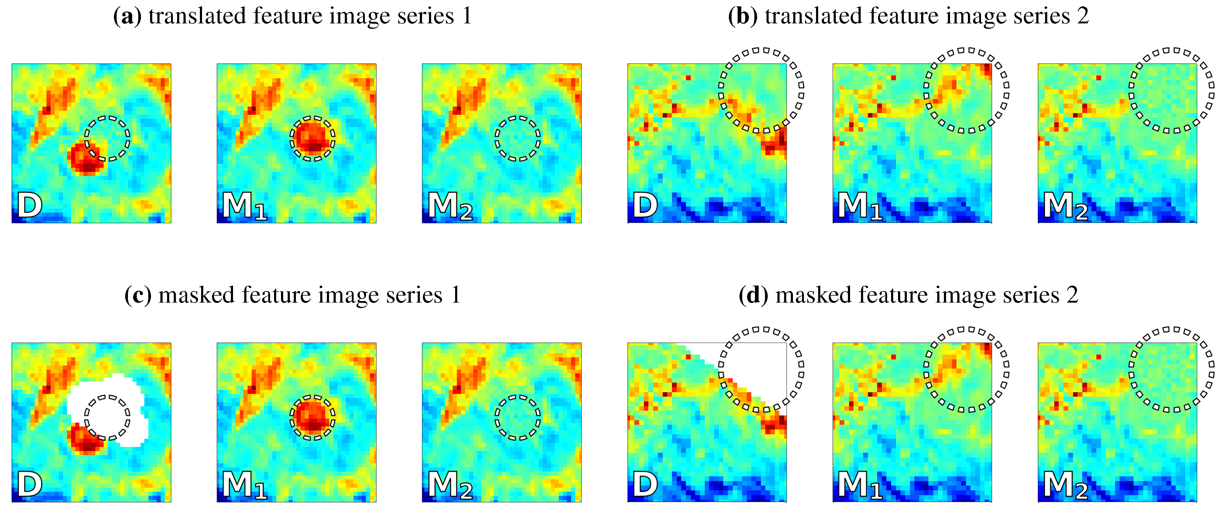
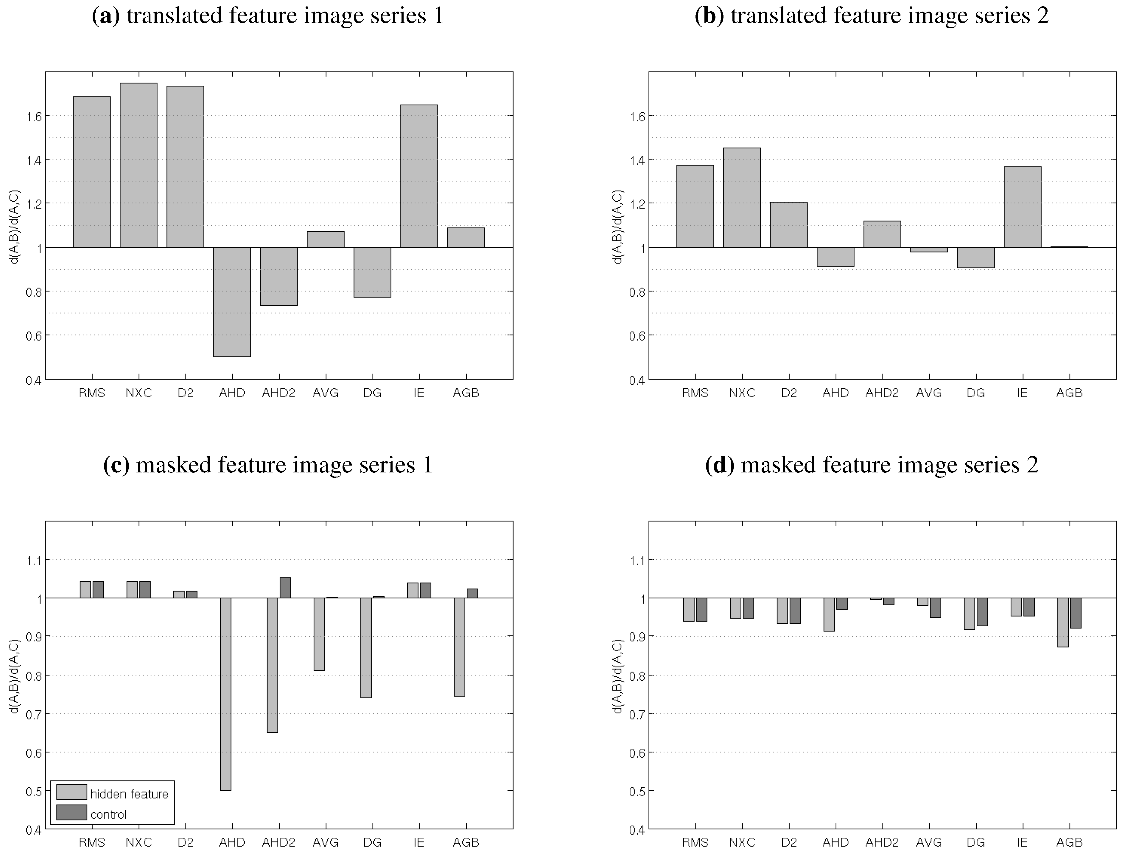
4.1. Test 1: Translated and Masked Features

In the first test, we explore whether the image comparison measures can detect translated and masked features in satellite images. For this purpose we introduce 3 images: D, $M_1$ and $M_2$. We assume that D is a satellite image that is compared to the model-derived images $M_1$ and $M_2$. In the first case, there is a feature that is present in both D and $M_1$, but at different locations; for example an eddy that is offset between data and model. This translated feature is not present in $M_2$ (see Figure 3 a,b). We consider it desirable for a distance measure d to rate D and $M_1$ to be closer than D and $M_2$, i.e., $d(D,M_1)<d(D,M_2)$, because of the common feature in D and $M_1$ that does not appear in $M_2$. In this case we prefer our model to show, as opposed to not show, a feature (e.g., the eddy) that appears in the satellite image, even if not at identical locations.

Figure 3. Examples of the manually created images used for the translated and the masked feature tests. In each test case, the first image represents the satellite image D which is compared to the images $M_1$ (center image) and $M_2$ (right image). D and $M_1$ share a common feature that does not appear in $M_2$. The location of this feature in $M_1$ is highlighted by a white dotted circle in every image. In the masked feature tests (c) and (d), this location is masked by $\mathit{NaN}$-values in D.

Figure 3. Examples of the manually created images used for the translated and the masked feature tests. In each test case, the first image represents the satellite image D which is compared to the images $M_1$ (center image) and $M_2$ (right image). D and $M_1$ share a common feature that does not appear in $M_2$. The location of this feature in $M_1$ is highlighted by a white dotted circle in every image. In the masked feature tests (c) and (d), this location is masked by $\mathit{NaN}$-values in D.

We use slightly modified versions of the above sets of images for the masked feature test, in which the satellite image D contains missing values at the same location where $M_1$ contains the feature. Figure 3 (c) and (d) show examples of D, $M_1$ and $M_2$ for the masked feature case. The feature is masked in $M_1$ if only pixels in $X_{\mathit{real}}$ are considered in the image comparison and therefore not accessible by pixel-by-pixel comparison measures. Yet, as both D and $M_1$ show the feature, we consider $d(D,M_1)<d(D,M_2)$ or the equivalent $\frac{d(D,M_1)}{d(D,M_2)}<1$ a desirable characteristic of d.

We applied the image comparison measures to the test cases presented in Figure 3. The results are shown in Figure 4 as ratios of $\frac{d(D,M_1)}{d(D,M_2)}$. For the masked feature test, Figure 4 also includes the results of a control experiment, where the pixels with missing values in D are set to missing values in $M_1$ and $M_2$, so that $D_{\mathit{NaN}}=M_{1,\mathit{NaN}}=M_{2,\mathit{NaN}}$. We further added a small amount of noise to all images in Figure 3, so that none of the distances are zero and $\frac{d(D,M_1)}{d(D,M_2)}$ retains a meaningful value.

Figure 4. Results of tests for the image series shown in Figure 3, expressed as ratios $\frac{d(D,M_1)}{d(D,M_2)}$. Ratios smaller than 1 are desirable

Figure 4. Results of tests for the image series shown in Figure 3, expressed as ratios $\frac{d(D,M_1)}{d(D,M_2)}$. Ratios smaller than 1 are desirable

In the cases with translated features, all pixel-by-pixel measures judge $M_2$ to be significantly closer to D than $M_1$, which is an inherent shortcoming of pixel-by-pixel comparison. For the neighborhood-based measures the results are more diverse: AHD and Delta-g show the most desirable results and clearly rate D and $M_1$ closer than D and $M_2$, while the results of IE are similar to those of RMS. The other measures fall in between, with $\frac{d(D,M_1)}{d(D,M_2)}$ close to 1.

For the cases with masked features, the pixel-by-pixel measures show the same pattern: $\frac{d(D,M_1)}{d(D,M_2)}$ has the same value for the sets of images used in the test cases and their respective control experiments ($\frac{d(D,M_1)}{d(D,M_2)}\ne 1$ because not the entire feature is masked), the masked feature does not have any effect. The neighborhood-based measures account for the masked feature to some degree, except for IE. For the masked feature image series 1 the distance of the two images is reduced significantly by the masked feature. For image series 2, this difference is not so obvious and the effect of the masked feature is insignificant or masked by noise.

The performance of the pixel-by-pixel measures is a direct result of not considering neighboring pixels. This also leads pixel-by-pixel measures to ignore the pixels in $D_{\mathit{NaN}}$ when comparing D to $M_1$ and $M_2$ in the masked feature case; consequently $\frac{d(D,M_1)}{d(D,M_2)}$ is the same for both, test and control experiment. All other methods compare pixels at different locations, which leads to an advantage in this test. Not all of the measures identify D to be closer to $M_1$, however. The individual results are also strongly dependent on the measures’ scaling parameters, an influence which we will return to in Section 5. The results of the masked feature test show clearly that the adapted comparison measures can make use of pixels in $D_{\mathit{NaN}}\cap M_{1,\mathit{NaN}}$ and that these pixels can change results significantly. The exception is our implementation of IE which is not a pixel-by-pixel measure but also ignores all pixels in $D_{\mathit{NaN}}$.

In this test we focused on the very specific scenario of a single translated/masked feature. The results are somewhat artificial as the images have been specifically created to be nearly identical except for the feature of interest. Nevertheless, translated and masked features can easily be caused by inconsistencies in the model (e.g., time lags) in conjunction with large areas of missing values.

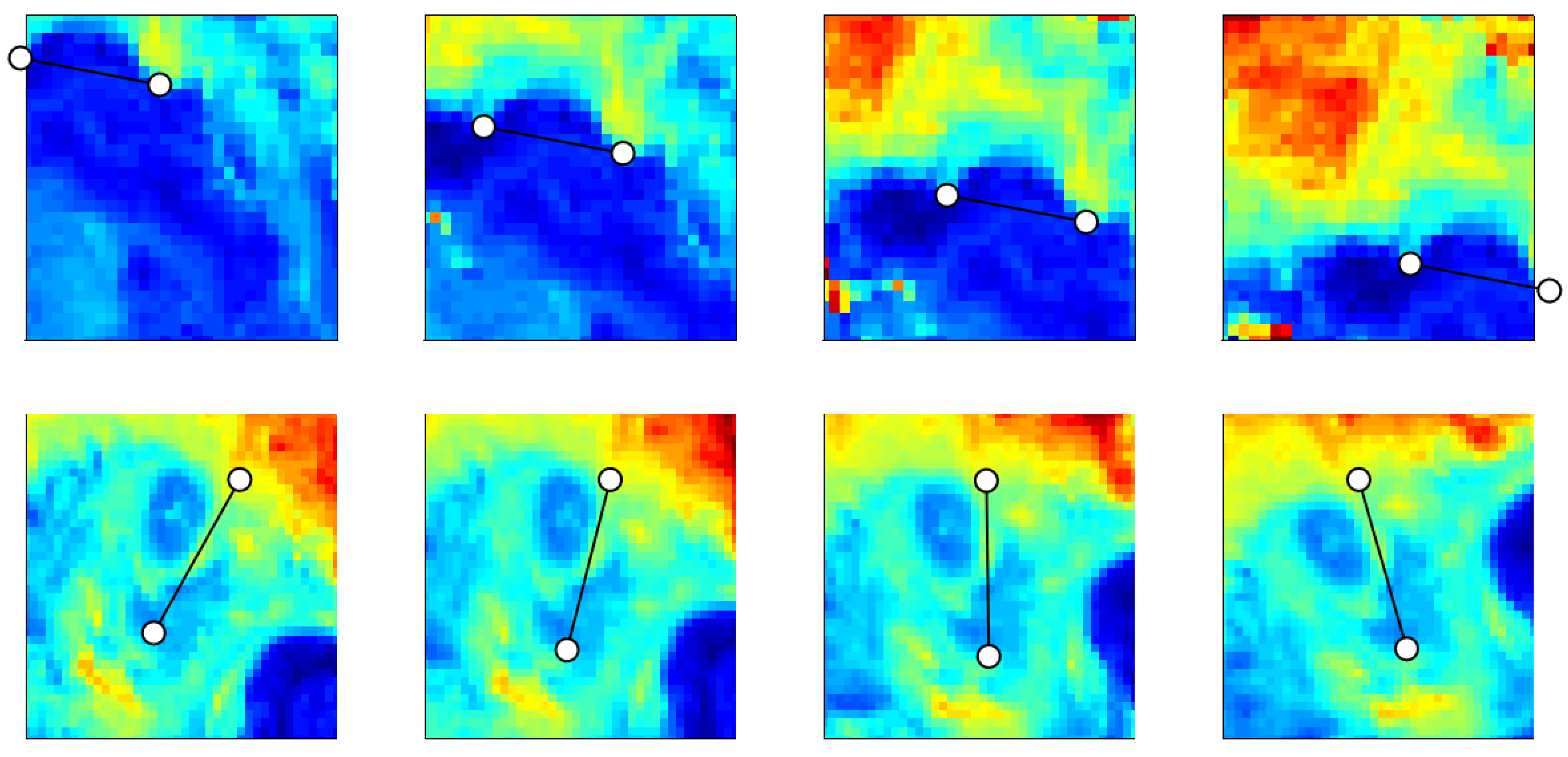
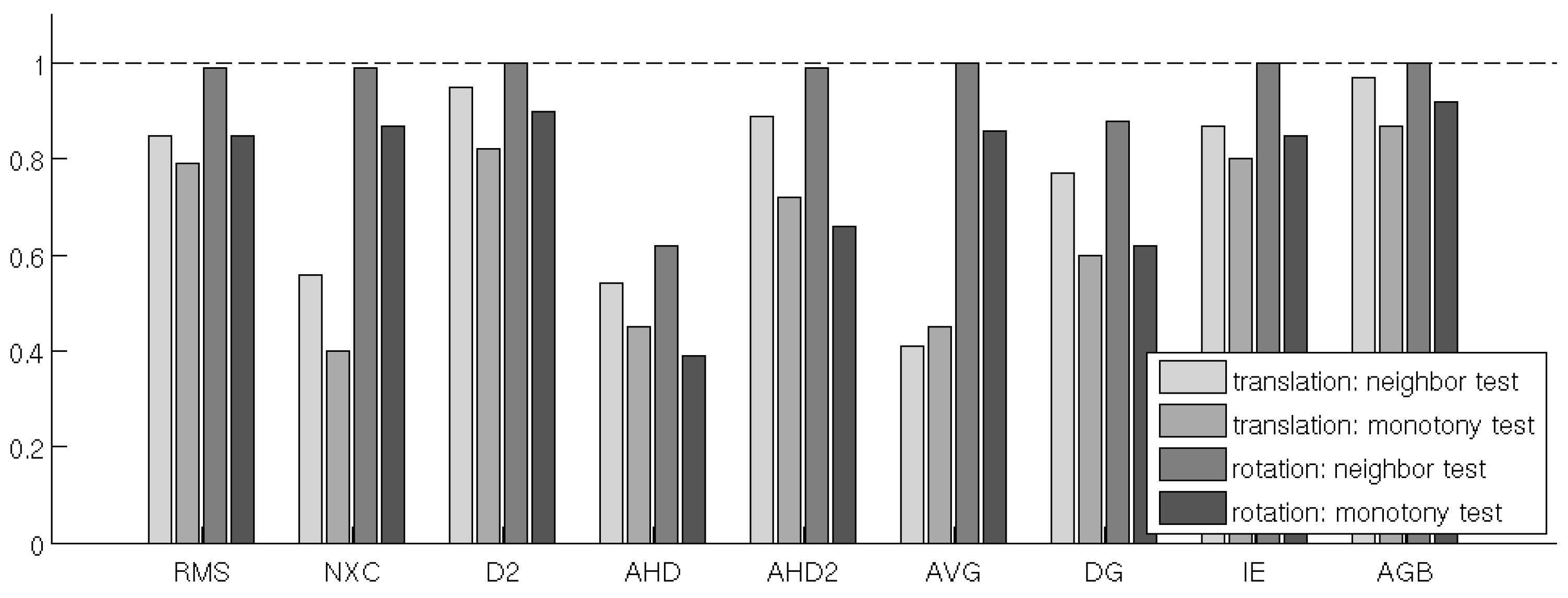
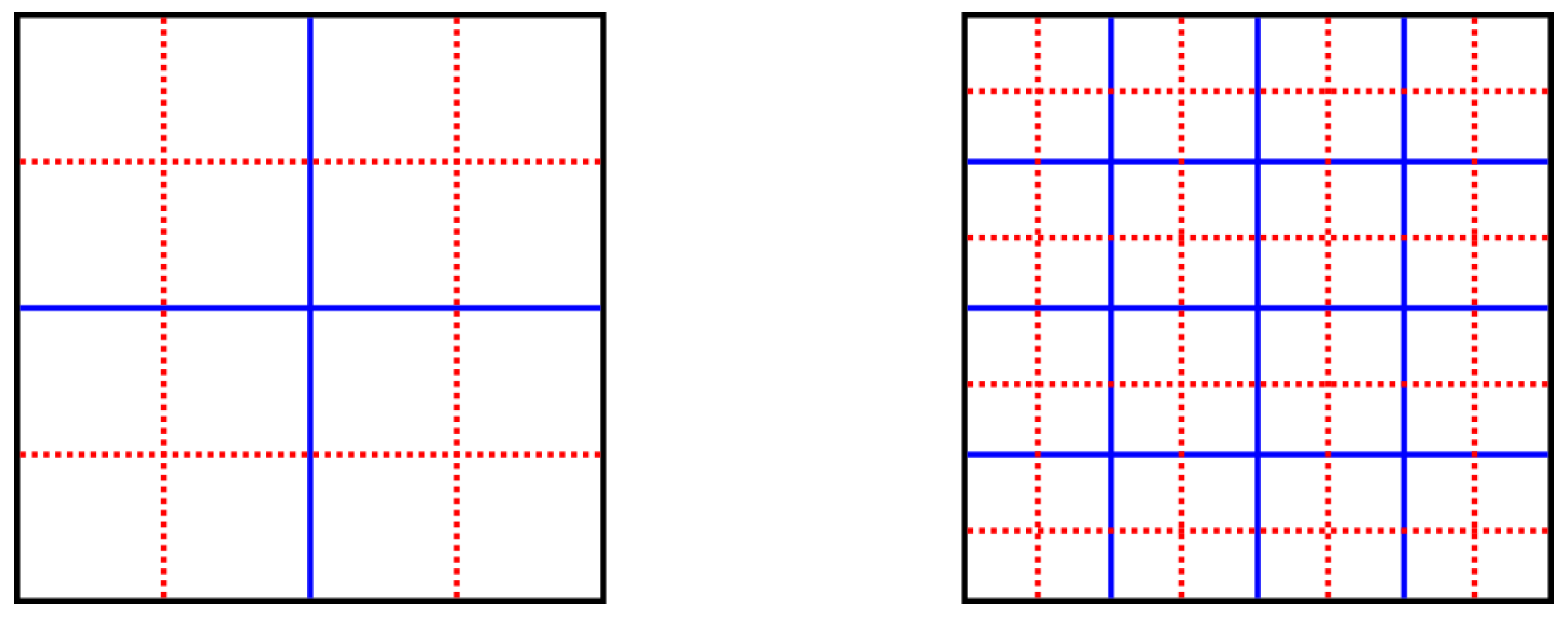
4.2. Test 2: Translation & Rotation of Images

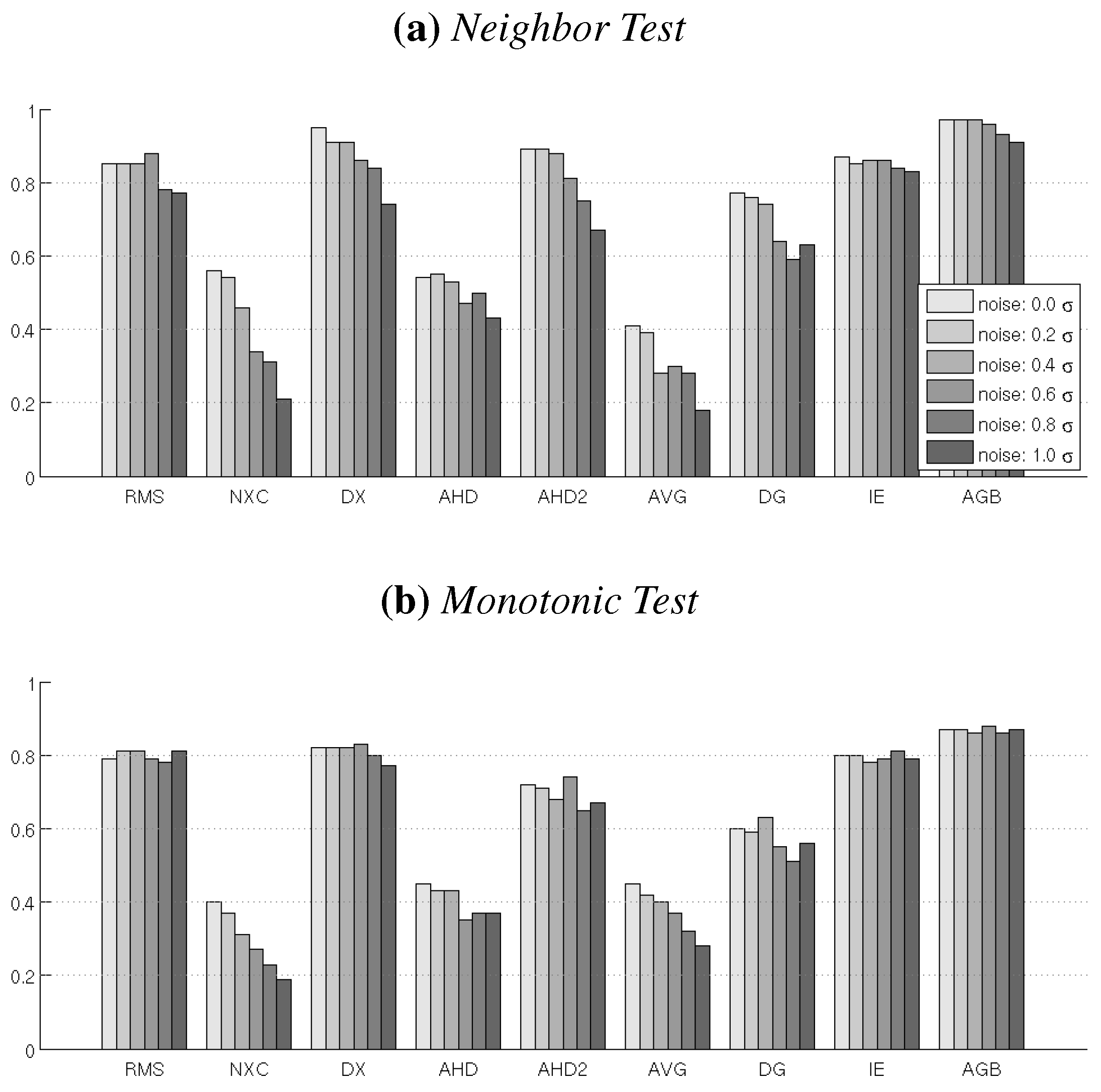
In this test we examine the effect of translation and rotation of a base image on the comparison measures. Stepwise translation or rotation of an image offers a simple way to create a series of similar images. Due to the nature of satellite images (as opposed to, e.g., images of white noise) an increased translation or rotation leads to an apparent increase in distance to the untransformed image. The image comparison measures should reflect this increase in distance.

For this test we generated a large number of series of transformed images. Starting with a large satellite image, each series was created by successively translating or rotating the image and then clipping it at the same position after each transformation. The clipping was done to ensure that the series contains no missing values that are introduced to the large image by the respective transformation. By adopting this approach we generated 100 series of translated images and 100 series of rotated images, each series containing between 5 and 6 images. Image sizes are constant within a series but range between $30\times 30$ and $50\times 50$ pixels among different series. The translations are performed along the X and Y axes as well as along their bisecting line. The translation distance between two images is 5 to 10 pixels. For each series of rotated images, the center of rotation is roughly in the center of the clipped image and the rotation angle between two images is 20${}^{\circ }$. In this test the images do not contain missing values and we do not add any noise to the images.

Given a series of increasingly translated or rotated images $A_1,A_2,\cdots ,A_q$ (e.g., see Figure 5) we perform two tests for each image comparison measure d:

neighbor test: 

A comparison measure d passes the neighbor test if for any given image in the series, the distance to one of the neighboring images in the series is smaller than the minimum distance to any non-neighboring image, i.e., if

$$\underset{j\in \{i-1,i+1\}}{min}d(A_i,A_j)<\underset{j\in \{1,\cdots ,i-2\}\cup \{i+2,\cdots ,q\}}{min}d(A_i,A_j)\mathrm{for}i=1,2,3,\cdots ,q$$

(25)

monotonic test: 

d passes the monotonic test if, for the first image in the series, the distance to the other images in the series is monotonically increasing, i.e., if

$$d(A_1,A_2)<d(A_1,A_3)<d(A_1,A_4)<\cdots <d(A_1,A_q).$$

(26)

Figure 5. A series of 4 translated images (top row) and a series of rotated images (bottom row) used in Test 2. Markers are inserted into the images to illustrate the direction of the translation and the angles of the rotation, respectively.

Figure 5. A series of 4 translated images (top row) and a series of rotated images (bottom row) used in Test 2. Markers are inserted into the images to illustrate the direction of the translation and the angles of the rotation, respectively.

Figure 6. Fractions of passed neighbor tests and monotonic tests for 100 series of translated and rotated images.

Figure 6. Fractions of passed neighbor tests and monotonic tests for 100 series of translated and rotated images.

The results of the two tests applied to both sets of images are shown in Figure 6. The ratio of passed tests is high for most distance measures, especially in the rotation neighbor test scenario. Generally, the results are better for the rotated images. This is especially obvious for AVG and NXC which have relatively low scores for the translated images, but perform roughly twice as well in the rotation test cases.

There is no indication that the pixel-by-pixel measures perform worse than the neighborhood-based methods, in fact RMS and D2 are among the best performing measures in all 4 test cases. It is interesting to note that the results of D2 are slightly better than those of the RMS. Among the neighborhood-based measures, AGB and IE perform well throughout all tests. The difference in parametrization among the two Hausdorff based measures is obvious, with AHD2 performing significantly better than AHD.

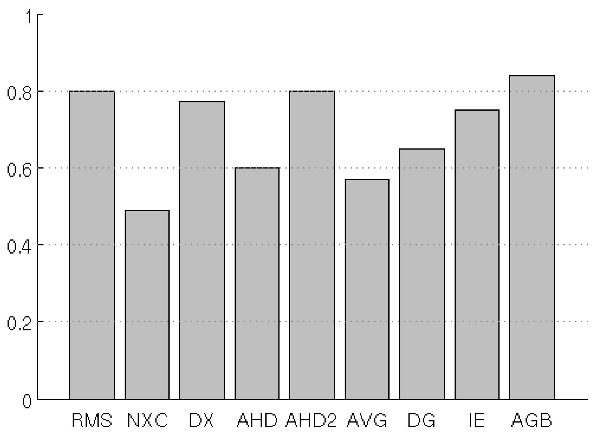
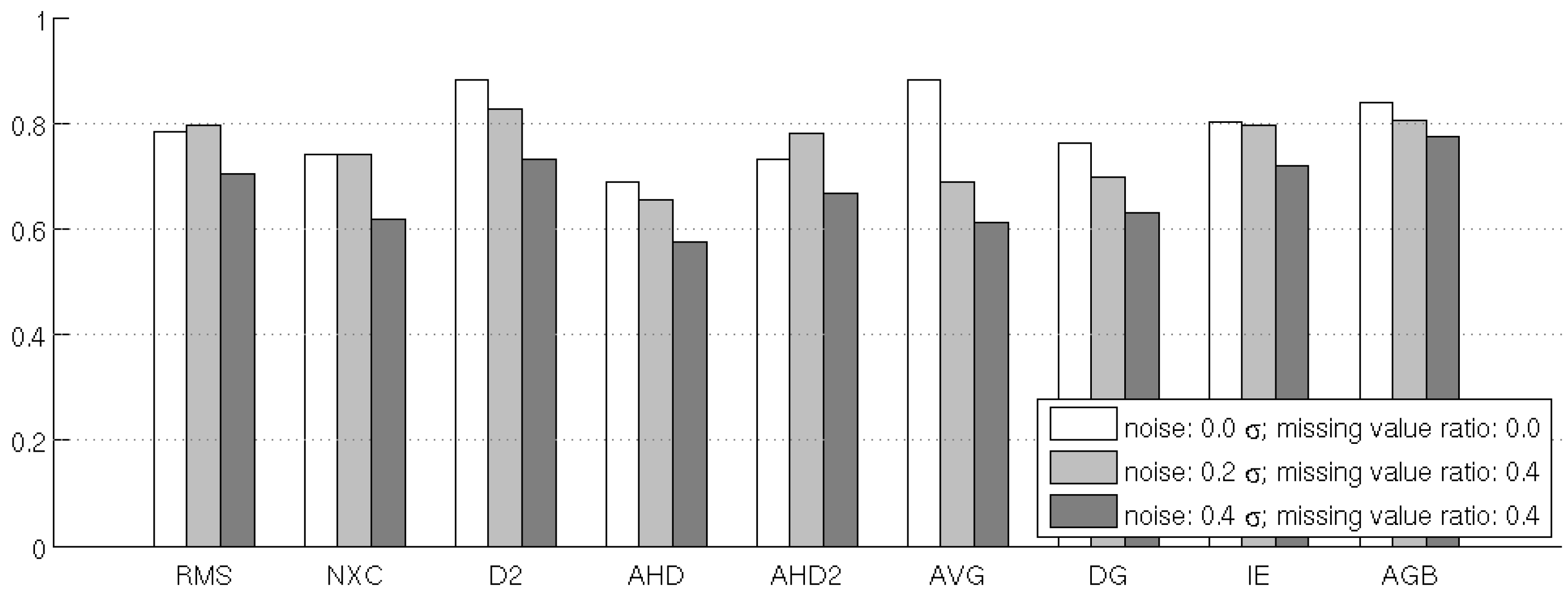
4.3. Test 3: Noise Sensitivity

In real life applications we expect that the satellite images contain some noise which may affect the image comparison. It is therefore important to test the noise sensitivity of image comparison methods. A multitude of publications have addressed this issue for regular gray scale images e.g.,[6]. To assess how variable levels of noise in images affect the satellite image comparison methods, we examine how the results from the previous test change under the influence of noise.

We used the 100 series of translated satellite images from the previous test. For each series, we determined the standard deviation σ of intensity values among all the images in the series. We then added Gaussian noise with mean 0 and standard deviation $x\sigma$ to each image (where adding the noise created negative values these were set to 0), where x is increased from 0.2 to 1.0 in increments of 0.2. For each noise level we performed the neighbor and monotonic test in the same manner as in the previous Test 2.

The results show that all comparison measures are affected by increased noise (Figure 7). The measures that employ averaging (AGB, IE and RMS) are the least sensitive to noise, with AGB performing best in both test cases. Especially the performance of AVG and NXC drops significantly as noise increases. D2 performed better than RMS at no noise, but drops below RMS with increasing noise. AHD and AHD2 exhibit a similar decline in performance compared to the no-noise results.

Figure 7. Fraction of Passed Neighbor Tests and Monotonic Tests for Different Levels of Noise.

Figure 7. Fraction of Passed Neighbor Tests and Monotonic Tests for Different Levels of Noise.

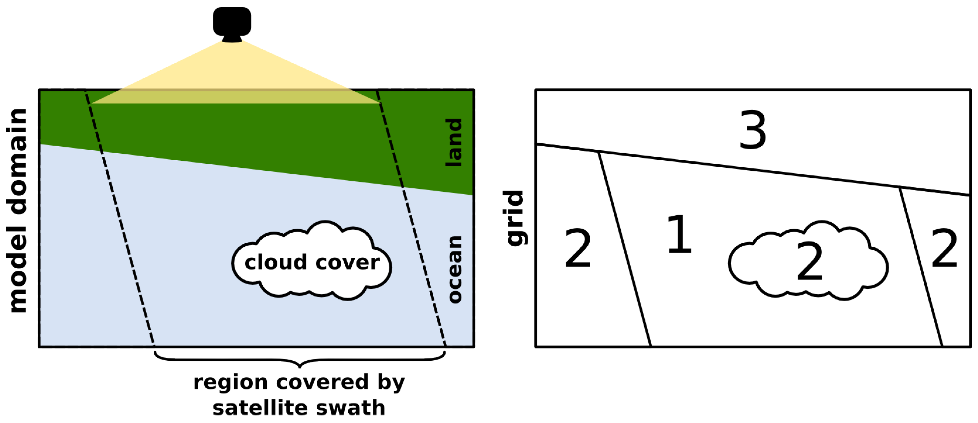
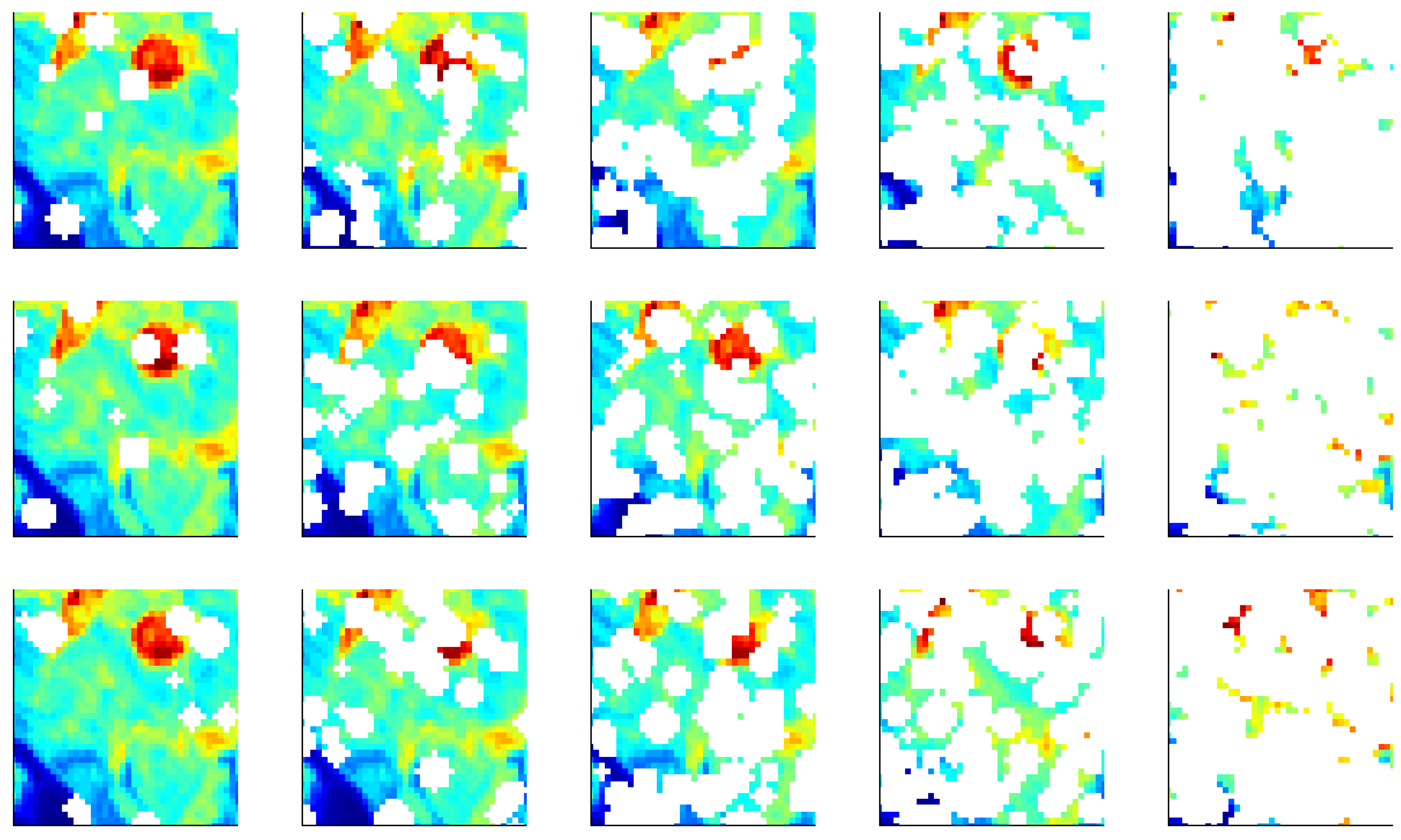
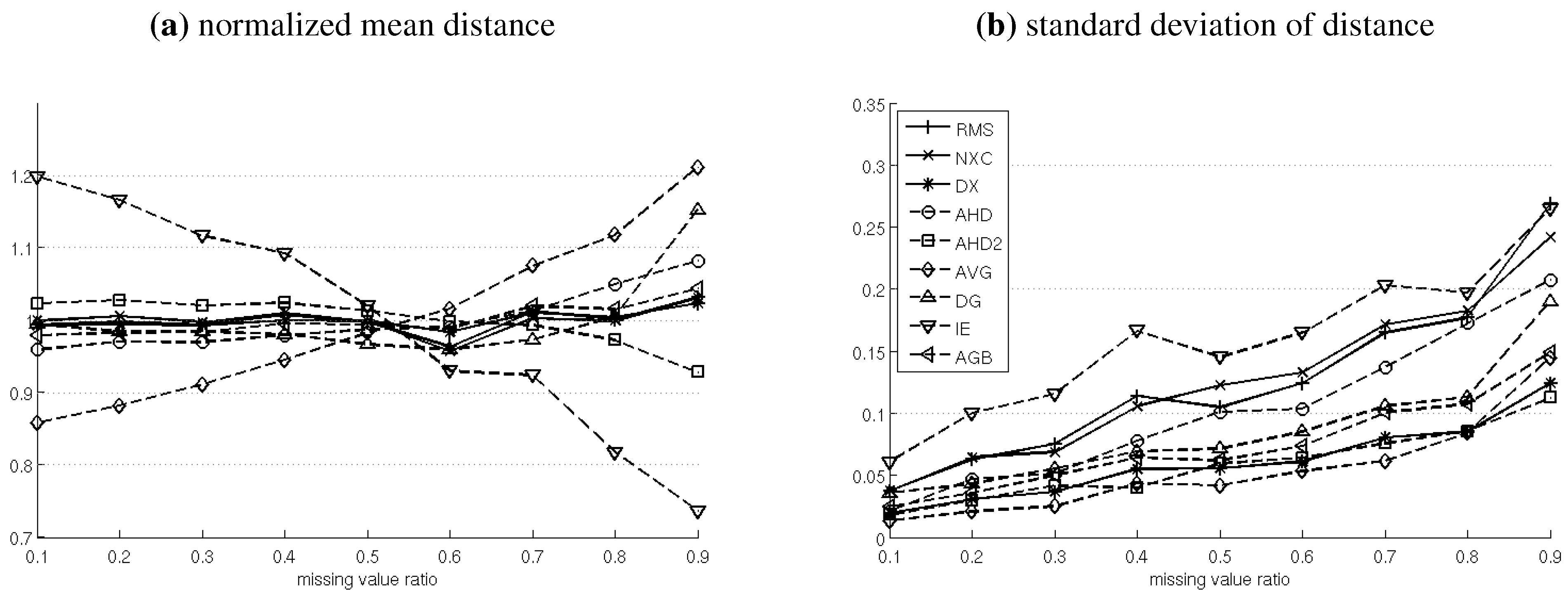
4.4. Test 4: NaN-Sensitivity

In addition to noise, missing values may also affect the performance of image comparison measures. In this test we examine the sensitivity of the image comparison measures to the location and number of missing values.

For this test we used two images of dimension $40\times 40$ and with a translation distance of 10 pixels from a series of translated images in Test 2. We then created 100 copies of the second image and selected a fraction $x_{\mathit{NaN}}$ of each copy to be missing values, varying $x_{\mathit{NaN}}$ from 0.1 to 0.9. The selection was performed in a way that creates uniformly distributed circles of missing values in the image, forming cloud-shaped areas (to mimic regions of missing values on optical ocean imagery), see Figure 8 for examples. Finally, we use the image comparison measures to compare the first image to all of the NaN-covered copies of the second image, computing 100 image distances for each comparison measure. We then record mean and standard deviation of distances (Figure 9).

Figure 8. 3 Realizations (Rows) of the Same Image Covered Randomly in Missing Values. From Left to Right the Number of Missing Values is Increased in Each Column from 10% to 90% in Increments of 20%.

Figure 8. 3 Realizations (Rows) of the Same Image Covered Randomly in Missing Values. From Left to Right the Number of Missing Values is Increased in Each Column from 10% to 90% in Increments of 20%.

The mean can be thought of as a measure of bias in this test: For a single realization of a randomly $\mathit{NaN}$-covered image, we can expect that a major feature is covered resulting in an increase or decrease of distance when compared to another image. While this makes it more likely that the distance diverts further from the mean as the number of missing values is increased, we do not expect the mean to change significantly with an increase in $x_{\mathit{NaN}}$ if the distance measure is unbiased. A significant change in mean implies that the distance measure is directly affected by the number of missing values and thus biased.

Figure 9. Mean and Standard Deviation of Image Distances for Different Levels of Missing Values. For Each Distance Measure, the Mean Values have been Normalized, so that Their Mean is 1.

Figure 9. Mean and Standard Deviation of Image Distances for Different Levels of Missing Values. For Each Distance Measure, the Mean Values have been Normalized, so that Their Mean is 1.

Noteworthy in this case are our adaptations IE and AVG which both show a significant bias. For IE, there is negative bias as the amount of missing values increases, lowering the mean distance. AVG, on the other hand, shows a positive bias, while the mean in all other distance measures is affected insignificantly.

The standard deviation in this test is a measure of missing value stability ($\mathit{NaN}$-stability). A lower standard deviation is desirable. It means that the distance between two images is less dependent on the location of missing values. The least stable distance measures, with highest standard deviations are IE, RMS and NXC. Measures that ignore pixels in $A_{\mathit{NaN}}\cap B_{\mathit{real}}$, with the exception of D2 which features one of the highest $\mathit{NaN}$-stabilities, show the worst performance in this test. They are followed by AHD which is significantly less NaN-stable than AHD2, illustrating the positive effect of its parametrization.

4.5. Test 5: NaN-Translation

In the previous test we assessed the sensitivity and stability of the image comparison measures when faced with missing values. Here, we examine the effects of missing values on the measures’ ability to correctly estimate relative distances between images.

We use again 100 series of translated images and randomly add missing values to the images, as described for Test 4. Using the monotonic test we compare the untouched image with the altered ones to test if the distance in the series increases. Because our previous results suggest that this test is significantly harder to pass than the monotonic test without missing values (Test 2) or under the influence of noise (Test 3), the image series in this test are slightly less translated (3 to 5 pixels in between individual images).

The results of this test (Figure 10) are similar to those of previous tests: our implementations of AGB, AHD2, RMS, D2 and IE perform well. NXC is the worst, passing less than half of the tests.

Figure 10. Fraction of passed monotonic tests for the NaN-translation case.

Figure 10. Fraction of passed monotonic tests for the NaN-translation case.

4.6. Test 6: Time-Series

All of the previous tests focused on the comparison of images that were generated by translating or rotating a base image or one of its features. In this final test we consider a numerical ocean model-generated time series of images. A time series poses a somewhat different challenge to the series of images generated through translation: Features appear and disappear in the center of the image (e.g., by upwelling) and features such as fronts and eddies not only change their location, which is the case with translated images, but also their shape and size. This test is closer to a realistic application than the previous ones.

We use images of model-simulated chlorophyll [taken from the model presented in 24]. Using a model to generate test images is advantageous because there are no missing values, no noise and the time interval between images can be selected. Also, we expect the images to exhibit similar features to satellite images.

For this test, we use 6 series of 31 images (with a time difference of 12 days between two consecutive images); the images are clipped and ranged in size from $40\times 50$ pixels to $70\times 150$ pixels among different series (Figure 11). Since the apparent distance of two images in a time series does not necessarily grow monotonically with time, we use a variation of the neighbor test in this scenario: We compare the distances of an image to its two neighbors with the distances to the other images within a window of 7 images, instead of all images (as done in Test 2). Performing a neighbor test for every image series, we obtain a ratio of passed to total tests for each series. The mean ratio and its standard deviation among the series are displayed in Figure 12 for different noise and missing value levels, which were added as described in Test 3 and 4, respectively.

Figure 11. An extraction of 4 consecutive images in a time series of images generated by a physical-biological ocean model.

Figure 11. An extraction of 4 consecutive images in a time series of images generated by a physical-biological ocean model.

Figure 12. Results of the time-series test. Bar height indicates average fraction of passed tests for the 6 time series of images.

Figure 12. Results of the time-series test. Bar height indicates average fraction of passed tests for the 6 time series of images.

The best performers in the test cases without noise or missing values are AVG, D2 and AGB. The results of AGB are only slightly affected by the addition of noise and missing values, while the performance of D2 and especially AVG drops considerably with increasing noise. Among the pixel-by-pixel measures, D2 achieves better results than RMS in all cases. The relatively good results of NXC indicate that there is a high level of correlation for neighboring images in the time series. For neighborhood-based measures, many results confirm previous observations: The parametrisation for AHD2 performs better than the one used in AHD. IE shows good performance that is not very sensitive to noise.

Table 2. Qualitative performance ratings of the image comparison measures for the 6 Tests in Section 4. The symbols indicate relative performance in the tests: + is good performance, ○ is average performance and – is bad performance.

Test	RMS	NXC	D2	AHD	AHD2	AVG	DG	IE	AGB
Test 1: translated & masked features	–	–	–	+	+	○	+	–	+
Test 2: translation & rotation	+	–	+	–	+	○	○	+	+
Test 3: noise sensitivity	+	–	+	–	○	–	–	+	+
Test 4: NaN-sensitivity	–	–	+	–	+	+a	○	–a	+
Test 5: NaN-translation	+	–	+	–	+	–	○	○	+
Test 6: time-series	○	–	+	–	○	○	–	○	+

^a The significant bias introduced through missing values is not included in the rating.

Table 2. Qualitative performance ratings of the image comparison measures for the 6 Tests in Section 4. The symbols indicate relative performance in the tests: + is good performance, ○ is average performance and – is bad performance.

Test	RMS	NXC	D2	AHD	AHD2	AVG	DG	IE	AGB
Test 1: translated & masked features	–	–	–	+	+	○	+	–	+
Test 2: translation & rotation	+	–	+	–	+	○	○	+	+
Test 3: noise sensitivity	+	–	+	–	○	–	–	+	+
Test 4: NaN-sensitivity	–	–	+	–	+	+a	○	–a	+
Test 5: NaN-translation	+	–	+	–	+	–	○	○	+
Test 6: time-series	○	–	+	–	○	○	–	○	+

^a The significant bias introduced through missing values is not included in the rating.

5. Discussion

For this study, we adapted 8 image comparison measures for use with satellite images. Our motivation was to compare satellite imagery with spatial fields derived from numerical ocean models, which has applications in model skill assessment and data assimilation. The distinguishing features of satellite images compared to regular images are that their values are continuous non-integer values and that pixels or portions can be missing. The examined comparison measures range from simple but widely used pixel-by-pixel methods to more complex methods that evaluate the distance of pixels at different locations. We compared the behavior of the comparison measures in 6 tests and assessed their response to different levels of noise and missing values. The qualitative performances of the measures are summarized in Table 2, and discussed in more detail below. One of our main goals was to compare the performance of the two very commonly used distance measures root mean square error and image correlation to lesser known alternatives.

Two measures outperformed both root mean square error and correlation throughout all of our tests. AGB, a neighborhood-based measure, achieved the best overall test results. It is especially insensitive to noise and missing values. The pixel-by-pixel measure D2 also achieved better results than the two commonly used methods, but is less advantageous in cases where translated or masked features play an important role (compare Test 1). In applications were runtime is not a primary concern, we recommend using AGB as distance measure. If low runtime is required, we recommend D2 over RMS.

Test 1 highlights the advantages of incorporating neighboring pixels into satellite image comparison; while the neighborhood-based methods can make use of the information in pixels that have values in the model but missing values in the data, the pixel-by-pixel measures cannot. Despite these inherent problems of pixel-by-pixel comparisons, the neighborhood-based measures are not always superior to the pixel-by-pixel measures. In Test 4, D2 distinguished itself from the other pixel-by-pixel measures by exhibiting a very high NaN-stability.

One important factor to consider is the parametrization of the image comparison measures. Every neighborhood-based measure we tested features one parameter or more. All of them contain a scaling parameter that weights the spatial distance of two pixels compared to their distance in intensity (the scaling parameters are listed in Table 1). Scaling parameters have a strong effect on the distance measures and the right choice depends on the resolution of the images that are compared. For high-resolution images, the distance between two neighboring pixels is low and spatial distance needs to be weighted lower in comparison to distance in intensity than for similar images with coarser resolution. A possible explanation for the good results of AVG in Test 6 in contrast to the average results in the other tests is that its scaling parameter matches the scale of model-generated images from Test 6 better than the scale of the satellite images used for tests 1–5.

Beside the scaling parameters, other parameters have significant effects on the results, too. A good example is the performance of AHD and AHD2, two parametrisations of the adapted Hausdorff distance. AHD2 performed better than AHD in all tests, due to a change of one parameter ($k_{\max }$) that controls the adapted Hausdorff distance’s proneness to extreme values.

A larger number of parameters allows for a high level of customization but has the negative side effect that parameters may need to be adapted for each application. Root mean square error and normalized cross-correlation have no parameters and thus do not require the user to select a specific parametrization. The customizability of the neighborhood-based measures varies strongly. The image Euclidean distance has only one parameter. The Hausdorff distance is highly customizable: Dubuisson & Jain [22] present 24 variations of the Hausdorff distance, some with their own parameters. Pixel-by-pixel measures can also have a high number of parameters, e.g. there are various flavors of entropic distances. The entropic distance $D_2$ used in this study is just one of 6 different entropic distances introduced in [17], each can be customized further.

Missing values are one of the distinguishing features of satellite images. Test 4 focused directly on the effects of the number of missing values on image distances. Bias introduced through missing values has different effects: In model skill assessment or data assimilation, bias is not an important issue since the number of missing values stays constant; one satellite image is compared to a number of model-derived images, each with the same number of missing values. Bias becomes important in scenarios where one image is compared to two or more images that have different number of missing values. NaN-stability, on the other hand, plays a more universal role and our results indicate that even for low ratios of missing values, the comparison measures display significantly different levels of NaN-stability. Here lies one of the apparent weakness of the standard pixel-by-pixel measures RMS and NXC which exhibit a very low NaN-stability.

All of our tests are based on the assumption that we can produce images that are less similar to one another by either moving a specific feature within the image, by increasing translation or rotation of the entire image, or by increasing the time difference of images in a time-series. This is done for a reason; apart from time-series and simple transformations, there is no easy way to create a set of images for which we have an objective indication of image similarity. Using any comparison measure as the basis for determining image similarity would be circular and predetermine the outcome of the tests.

Beside test performance, ease of implementation and runtime need to be considered. The pixel-by-pixel measures are generally very easy to implement and they are the fastest methods. Because they compare only pixels at the same location they have a complexity O$\left(mn\right)$. All neighborhood-based measures have a higher complexity and, due to their more elaborate means of comparing pixels at different locations, are also harder to implement. The variation in runtime and ease of implementation among them is significant. One of the fastest neighborhood-based measures we tested is AGB. It has a complexity of roughly O$\left({log}_2(max(m,n))max{(m,n)}^2\right)$. AVG is the only other neighborhood-based measure with a complexity below O$\left({\left(mn\right)}^2\right)$, although its runtime is strongly dependent on its parametrization. The slowest methods are AHD, IE and DG; runtime of the latter is also very dependent on the choice of parameters. Ease of implementation is not as easy to judge objectively. We found image Euclidean distance and adapted Hausdorff distance to be the easiest to implement while an efficient implementation of average distance, adapted gray block distance and especially Delta-g took more effort.

6. Conclusions

This study shows that low level image comparison measures, developed for regular gray scale images, can successfully be adapted to work with satellite images. In comparison to standard comparison measures such as root mean square error (RMS) and cross-correlation, two of our adapted measures show better performance throughout all of our tests. These measures are the adapted gray block distance (AGB), which compares images at multiple scales, and the entropy based measure $D_2$. The advantages of these measures are especially apparent in scenarios that involve missing values, one of the distinguishing features of satellite images. AGB also exhibits the lowest sensitivity to noise among the measures we tested and we would therefore recommend it over RMS. While AGB requires more runtime than pixel-by-pixel measures, it is among the fastest neighborhood-based methods we tested. In cases where runtime or ease of implementation are the prime concerns, the pixel-by-pixel measure $D_2$ is still a better alternative to RMS.

References

1. Allen, J.; Holt, J.; Blackford, J.; Proctor, R. Error quantification of a high-resolution coupled hydrodynamic-ecosystem coastal-ocean model: Part 2. Chlorophyll-a, nutrients and SPM. J. Marine Syst. 2007, 68, 381–404. [Google Scholar] [CrossRef]
2. Stow, C.; Jolliff, J.; McGillicuddy, D.; Doney, S.; Allen, J.; Friedrichs, M.; Rose, K.; Wallhead, P. Skill assessment for coupled biological/physical models of marine systems. J. Marine Syst. 2009, 76, 4–15. [Google Scholar] [CrossRef]
3. Lehmann, M. K.; Fennel, K.; He, R. Statistical validation of a 3-D bio-physical model of the western North Atlantic. Biogeosciences 2009, 6, 1961–1974. [Google Scholar] [CrossRef]
4. Bennett, A. Inverse Modeling of the Ocean and Atmosphere; Cambridge University Press: Cambridge, UK, 2002. [Google Scholar]
5. Dowd, M. Bayesian statistical data assimilation for ecosystem models using Markov Chain Monte Carlo. J. Marine Syst. 2007, 68, 439–456. [Google Scholar] [CrossRef]
6. Avcıbaş, İ.; Sankur, B.; Sayood, K. Statistical evaluation of image quality measures. J. Electron. Imag. 2002, 11, 206–245. [Google Scholar]
7. Mannino, A.; Russ, M.; Hooker, S. Algorithm development and validation for satellite-derived distributions of DOC and CDOM in the US Middle Atlantic Bight. J. Geophys. Res. 2008, 113, C07051. [Google Scholar]
8. Lehmann, T.; Sovakar, A.; Schmiti, W.; Repges, R. A comparison of similarity measures for digital subtraction radiography. Comput. Biol. Med. 1997, 27, 151–167. [Google Scholar] [CrossRef]
9. Le Moigne, J.; Tilton, J. Refining image segmentation by integration of edge and region data. IEEE T. Geosci. Remote Sens. 1995, 33, 605–615. [Google Scholar] [CrossRef]
10. Alberga, V. Similarity measures of remotely sensed multi-sensor images for change detection applications. Remote Sens. 2009, 1, 122–143. [Google Scholar] [CrossRef]
11. Holyer, R.; Peckinpaugh, S. Edge detection applied to satellite imagery of the oceans. IEEE T. Geosci. Remote Sens. 1989, 27, 46–56. [Google Scholar] [CrossRef]
12. Cayula, J.; Cornillon, P. Edge detection algorithm for SST images. J. Atmos. Ocean. Tech. 1992, 9, 67–80. [Google Scholar] [CrossRef]
13. Belkin, I.; O’Reilly, J. An algorithm for oceanic front detection in chlorophyll and SST satellite imagery. J. Marine Syst. 2009, 78, 319–326. [Google Scholar] [CrossRef]
14. Nichol, D. Autonomous extraction of an eddy-like structure from infrared images of the ocean. IEEE T. Geosci. Remote Sens. 1987, 25, 28–34. [Google Scholar] [CrossRef]
15. Santini, S.; Jain, R. Similarity measures. IEEE T. Pattern Anal. 1999, 21, 871–883. [Google Scholar] [CrossRef]
16. Di Gesú, V.; Starovoitov, V. Distance-based functions for image comparison. Pattern Recog. Lett. 1999, 20, 207–214. [Google Scholar] [CrossRef]
17. Di Gesú, V.; Roy, S. Pictorial indexes and soft image distances. Springer: Berlin/Heidelberg, Germany, 2002; pp. 63–79. [Google Scholar] [CrossRef]
18. Huttenlocher, D.; Klanderman, G.; Rucklidge, W. Comparing images using the Hausdorff distance. IEEE T. Pattern Anal. 1993, 15, 850–863. [Google Scholar] [CrossRef]
19. Wilson, D.; Baddeley, A.; Owens, R. A New Metric for Grey-Scale Image Comparison. Int. J. Comput. Vision 1997, 24, 5–17. [Google Scholar] [CrossRef]
20. Wang, L.; Zhang, Y.; Feng, J. On the Euclidean distance of images. IEEE T. Pattern Anal. 2005, 27, 1334–1339. [Google Scholar] [CrossRef] [PubMed]
21. Juffs, P.; Beggs, E.; Deravi, F. A multiresolution distance measure for images. IEEE Sig. Proc. Lett. 1998, 5, 138–140. [Google Scholar] [CrossRef]
22. Dubuisson, M.; Jain, A. A modified Hausdorff distance for object matching. In Proceedings of the 12th IAPR International Conference on Computer Vision & Image Processing, Jerusalem, Israel, 1994; pp. 566–568.
23. Sim, D.; Kwon, O.; Park, R. Object matching algorithms using robust Hausdorff distance measures. IEEE T. Image Proc. 1999, 8, 425–429. [Google Scholar]
24. Fennel, K.; Wilkin, J.; Previdi, M.; Najjar, R. Denitrification effects on air-sea CO2 flux in the coastal ocean: simulations for the Northwest North Atlantic. Geophys. Res. Lett. 2008, 35, L24608. [Google Scholar] [CrossRef]