Monitoring Automotive Particulate Matter Emissions with LiDAR: A Review

Abstract

Automotive particulate matter (PM) causes deleterious effects on health and visibility. Physical and chemical properties of PM also influence climate change. Roadside remote sensing of automotive emissions is a valuable option for assessing the contribution of individual vehicles to the total PM burden. LiDAR represents a unique approach that allows measuring PM emissions from in-use vehicles with high sensitivity. This publication reviews vehicle emission remote sensing measurements using ultraviolet LiDAR and transmissometer systems. The paper discusses the measurement theory and documents examples of how these techniques provide a unique perspective for exhaust emissions of individual and groups of vehicles.

1. Introduction and Background

Gases and particulate matter (PM) emitted by vehicles can greatly affect ambient air quality and have direct implications for human health [1], climate change [2], visibility [3], ecosystem productivity [4], and artistic and historic buildings preservation [5], all with consequences for society and national safety and security. Pollutants emitted by vehicles are typically regulated by government agencies (e.g., the US Environmental Protection Agency in the USA) and typically include: carbon monoxide (CO) and hydrocarbons (HC) (emitted during fuel-rich combustion conditions), nitrogen oxides (NO) (emitted during high-temperature combustion conditions), and PM. In the last few years the interest in PM emissions has grown substantially due to both air quality issues and the co-effects of new PM emission regulations on global and regional radiative forcing and therefore climate change [6,7].

Measuring PM emission factors of vehicles represents a major technical and scientific challenge due to the complexity of PM physical and chemical properties including PM shape and size distribution, chemical composition and mixing state (i.e., internal vs. external). These properties are affected by interactions with the environment and change with time after emission. Most of the PM mass from vehicle exhaust is characterized as (1) Organic carbon (OC) PM composed of a complex mixture of organic compounds that are generally weak light-absorbers and form particles of spherical shape (i.e., white smoke) and (2) black carbon (BC) PM, consisting of fractal-like aggregates of smaller quasi-spherical carbon monomers with disordered crystalline or amorphous carbon structure (i.e., soot or black smoke). As indicated by its name, BC PM strongly absorbs visible and near visible light [8,9] with a very large mass absorption efficiency, which has been estimated to be on the order of 7.5 ± 1.2 m²/g [10]. These two types of particles might be internally and/or externally mixed in emissions from an individual vehicle and their mixing increases with longer permanence in the atmosphere, especially when exposed to other pollutants.

A LIght Detection And Ranging (LiDAR) approach to measure vehicle PM emissions in realistic conditions was recently developed and employed to measure the distribution of emissions of many 1,000s of vehicles. This paper reviews the remote sensing system [11], the theory of operation [12], and its use in multiple field campaigns [13,14,15,16,17,18].

The review is organized in five sections: in the remaining part of Section 1 (introduction and background) we introduce, in a general manner the problem of vehicle emission measurements and the technical challenges and possible approaches. In Section 2, we describe the theoretical framework used to quantify the vehicle emission factors in terms of mass of pollutant emitted by each individual vehicle per mass of fuel consumed. In Section 3, we enter into the details of the specific UV LiDAR and transmissometer system that is the subject of this review and that was developed for the on-road quantification of PM emission factors. Section 3 includes a discussion of the apparatus, the noise and sources of uncertainty, and the theory used to convert the optical measurement into a PM mass concentration and/or column content. A specific example drawn from an on-road deployment of the system is used to illustrate the procedure followed for the emission factor calculation. Results from a field validation study are also presented. In Section 4, we describe some selected results from a couple of field campaigns using the UV LiDAR and transmissometer system in conjunction with a gaseous remote sensing system. Section 5 summarizes the different topics discussed and concludes the review.

1.1. Vehicle Emissions

Variability of vehicle exhaust emissions stems from many complicating and confounding factors including for example, but not limited to: (a) wide variety of vehicle and engine types; (b) vehicle use and maintenance; (c) vehicle operating conditions; (d) vehicle age; (e) fuel type and quality; (f) driving habits; (g) weather conditions; (h) road conditions; (i) traffic conditions; (j) enforcements of inspection and maintenance programs or other emission control programs. Due to the large number of parameters and the wide range of variability for each, it is difficult to obtain a representative and statistically relevant sample of vehicle emission factors. To make the task even more formidable, the emission distribution across the vehicle fleet is often strongly skewed, making a few vehicles responsible for the largest fraction of the total fleet emissions. The emission distribution skewness has been shown to be especially severe for CO and PM emissions with ~10% of the vehicles contributing more than 70% of the total fleet emissions for passenger cars [14,19,20]. Therefore, normal parametric statistical approaches are prone to bias, especially when sample counts are low (i.e., <1,000 vehicles). Large samples sets are needed to accurately capture the tail of the emission distribution and to stratify emissions by the different confounding variables.

An effective strategy to quantify and then reduce the deleterious effects of vehicle emissions needs to be two-fold: first, detailed emission inventories need to be assembled using measurements from broad geographical areas; second, a reliable prediction tool needs to be developed to estimate future emissions and to infer vehicle exhaust emissions in areas where emission measurements are not available. In both cases—database and model development—a measurement approach needs to be developed to overcome the difficulties related to the multi-parameter problem mentioned above. No individual measurement technique is currently available that can precisely stratify these parameters. In addition, emissions are also continuously changing in response to societal dynamics, emission control strategies, and technological advances.

The need for remote sensing of automotive PM emissions is made more urgent by the fact that the PM emission factors from passenger cars are skewed and that this skewness will likely become more severe with technology improvements on later model years and with more stringent regulatory policies. This necessitates the development of reliable technology to detect the very few gross emitters in large in-use fleets.

1.2. Measurement Challenges

Many approaches have been explored and developed over the years to measure exhaust emissions from vehicles. Laboratory studies are probably the most controlled and therefore most accurate and precise methods, however the cost and time needed for the measurement of an individual vehicle strongly limit the sample size (in terms of number of total vehicles) that is realistically achievable. In addition, it is difficult to attain and demonstrate the ability to accurately reproduce real-world conditions in the laboratory. Techniques, such as tunnel studies, can provide large sample sizes, but vehicle specificity is compromised and the availability of suitable and representative locations is severely limited [21,22]. Partial solutions to the representativeness of “real-world conditions” are provided by chase studies [23,24] and on-board measurements [25,26], but both of these techniques still suffer from the practical limitations to obtain large and statistically representative samples.

Among the many techniques available for vehicle emission measurements, remote sensing (i.e., measurement of optical scattering and/or extinction across an active roadway) presents a unique set of advantages. First, remote sensing offers the possibility to collect data for thousands of vehicles at a reasonable cost, and with modest time and human resource investments. Second, remote sensing is the only currently available technique that is able to collect data representative of a large and realistic ensemble of vehicles, maintaining at the same time the specificity of “single vehicle” emission measurement via images of the vehicle’s license plate [27]. Remote sensing also incorporates a set of restrictions that limit its applicability. For example, remote sensing captures just a “snapshot” of the emissions of each vehicle, generally represented by just a half a second measurement [28]. In addition, as is true of most remote sensing techniques, vehicle remote sensing is limited to the use of electromagnetic radiation as a sensing tool.

Before remote sensing became available for vehicle emissions however, little was known about the statistical distribution of real-world vehicle exhaust emissions [20]. Distribution information is useful to determine contributions from different fleet segments (e.g., high emitters, older vehicles) and the variability of emissions within a subcategory (e.g., model year). Some studies have integrated remote sensing with roadside, dynamometer or on-board testing or tunnel studies in a hybrid approach that can exploit the unique advantages of the different techniques (e.g., using remote sensing to identify high emitters) and combine the strengths of the individual methods [29,30,31].

1.3. Vehicle Emission Remote Sensing Systems

Vehicle emissions remote sensing systems (VERSSs) can measure gaseous emission factors for large numbers of individual vehicles (on the order of 1,000 vehicles per hour) by deploying light sources and detectors on the road-side on a single lane road. Suitable sites are often on-ramps of freeways or congested urban roads where the traffic passing through the optical beam is accelerating and has been restricted to a single lane by using traffic cones and signals.

Gaseous VERSSs measure infrared (mostly for carbon dioxide, carbon monoxide and hydrocarbons) and ultraviolet (mostly for nitrogen oxide) extinction across the road to quantify the mass column content of the gases of interest [31,32,33,34,35,36,37,38,39,40,41,42,43,44,45]. Often an infrared (IR) source and an ultraviolet (UV) lamp are placed on one side of the road together with a set of bandpass filters and a detection system. On the opposite side of the road, a retroreflector is installed to allow a double pass of the IR and UV radiation through the plume. Mass column content is a two-dimensional mass density (with dimension of mass/area) of the emitted gas of interest. The total carbon mass content in the vehicle exhaust is mostly in the form of carbon dioxide (CO₂) and some CO and HC, and it is used to calculate fuel-based emission factors (EFs).

The remote sensing measurements have a high temporal resolution (~10 ms) to yield multiple sampling (typically 20–50 samples) before and after the vehicle passes through the sensor. The sampling done immediately before the vehicle passes through the sensor is used to estimate the ambient background. It is assumed that during the short time of the measurement the background remains substantially unchanged. The accuracy of this assumption is quantified for each individual vehicle by calculating the standard deviation of the 20 measurements collected immediately before the vehicle passed through the system; if the standard deviation is larger than a threshold specified by the operator, the measurement is flagged as invalid (e.g., in the case of a plume from a previous car not yet dissipated).

2. Fuel-Based Pollutant Emission Factors Calculation

Since the carbon mass fraction of automotive fuel is known, the ratio of the two mass column contents (the pollutant column content and the total carbon column content) can be used to calculate the mass emission of the pollutant of interest per mass of fuel consumed, yielding a fuel-based emission factor [11]. This emission factor (EF_P) for pollutant (P) is defined as the ratio of the mass of pollutant emitted (M_P) per mass of fuel consumed (M_fuel):

$$E{F}_P=\frac{M_P}{M_{fuel}}$$

(1)

Defining CMF_fuel as the carbon mass fraction of the fuel (i.e., the carbon mass of the fuel (CM_fuel) divided by its mass (M_fuel)), the fuel mass (M_fuel) can be replaced, yielding

$$E{F}_P=CM{F}_{fuel}\frac{M_P}{C{M}_{fuel}}$$

(2)

The carbon mass emitted by the vehicle equals the carbon mass of the fuel consumed (carbon balance). Thereby, the fuel carbon mass (CM_fuel) can be replaced by the carbon mass of the exhaust, which is the sum of the mass of its main carbon-containing components, weighted by their respective carbon mass fraction:

$$\begin{array}{l}E{F}_P=CM{F}_{fuel}\frac{M_P}{C{M}_{exhaust}}=CM{F}_{fuel}\frac{M_P}{{\displaystyle \sum _{i}C{M}_i}}=CM{F}_{fuel}\frac{M_P}{{\displaystyle \sum _{i}CM{F}_i\cdot M_i}}\\ =CM{F}_{fuel}\frac{{\rho }_{c-P}}{{\displaystyle \sum _{i}CM{F}_i\cdot {\rho }_{c-i}}}\end{array}$$

(3)

where the mass ratios have been replaced by the ratios of the respective exhaust mass column contents (ρ_c-P and ρ_c-i) as measured by a VERSS. Expanding the sum over the main carbon-containing components of gaseous emissions (i.e., CO₂, CO, and HC) and dividing the numerator and denominator by the CO₂ mass $M_{C{O}_2}$ yields [11]:

$$E{F}_P=CM{F}_{fuel}\frac{\frac{{\rho }_{c-P}}{{\rho }_{c-C{O}_2}}}{CM{F}_{C{O}_2}+\left(CM{F}_{CO}\frac{{\rho }_{c-CO}}{{\rho }_{c-C{O}_2}}+CM{F}_{HC}\frac{{\rho }_{c-HC}}{{\rho }_{c-C{O}_2}}\right)}$$

(4)

where the terms in parentheses may be neglected for most vehicles with the exception of gross CO or HC emitters. The contribution of particulate carbon emissions is even less significant and has been neglected from the denominator in Equation (4). The fuel-based EF_P can be determined from a VERSS measurement of the mass column contents ρ_c using Equation (4), if the carbon mass fractions (CMF) are known. For CO and CO₂, CMFs can be calculated directly from the respective atomic masses yielding CMF_CO = 42.9% and $CM{F}_{C{O}_2}$ = 27.3%. For fuels, one may assume empirical formulas of C_nH_1.825n for gasoline and C_nH_2n for diesel, resulting in CMF_gasoline = 86.7% and CMF_diesel = 85.6% [46].

If PM is the pollutant of interest and its mass column content can be measured simultaneously with the carbon mass column content, fuel-based PM emission factors can be determined using the same methodology used for gaseous emission factors. Chen et al. [47] demonstrate how the PM closely follows the gas molecules in the plume while dispersed by turbulence, with negligible deviations during the short sampling time. While measurements of gaseous on-road emissions with remote sensors have become routine, VERSS technology to measure on-road PM emission factors has not been available until recently.

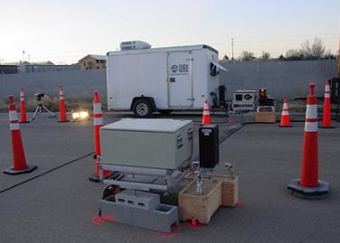
3. UV LiDAR and Transmissometer System for Vehicle PM Emission Measurements

3.1. Measurement Approach and Instrument Design

As described in the previous section, fuel-based PM EFs can be calculated from PM mass column content (PM mass concentration intergraded over the path length) that has been measured simultaneously with the carbon mass column content measured by gaseous VERSS [11]. Properties of automotive PM emissions such as PM chemical composition, size distribution, internal/external mixing, particle shape, and refractive indices of components vary as a function of engine, fuel, exhaust system, and operating conditions, and influence their optical properties. A PM sensor should measure PM mass column content with a small dependence on these variables within their normal range; deviations should be minimized and quantified to yield an instrument of known accuracy. Calculations of the optical properties of automotive PM and their sensitivity to different parameters are reported in the next sections.

3.1.1. State of the Art

Optical opacity can be used to estimate PM mass column content although this approach is quantitatively challenging since the light extinction associated with moderately emitting vehicles may be very small; the method is mostly suitable for diesel vehicles. Chen et al. [47] for example demonstrate the feasibility of an opacity-based PM remote sensing unit by measuring opacity at 710 nm from a diesel vehicle and a diesel bus in a laboratory setting. Morris et al. [48] report road side IR (3.9 μm) opacity data for 314 measurements on individual heavy-duty diesel trucks and found a correlation with the CO EFs. Stedman and Bishop [49] reported encouraging results on the identification of gross PM emitters using a combination of three opacity measurements, a UV channel (using an ultraviolet xenon arc lamp with a bandpass filter at 240 nm), a visible channel (using a He/Ne laser at 632.8 nm), and an IR channel (using a thermal source with a bandpass filter at 3.9 μm) [42]; the experiment was carried out characterizing emissions from three light duty diesel trucks [49].

A more sensitive method to measure PM EFs from individual vehicles is to detect the light backscattered from the PM in the vehicle exhaust. For this application, a LiDAR approach needs to be employed to properly account for the variable spatial distribution and location of the vehicle plume and for the range-dependence of the backscattered signal. An interesting development, based on intensity-modulated, stepped frequency CW LiDAR, was proposed by Simpson et al. [50]. The system, based on CW laser diode operating at 660 nm, showed potential for its low cost and simplicity; however, to our knowledge, data and analysis from the operational on-road deployment of the system are not currently publicly available. A different approach was taken by Koren and Eichinger [51]; they used a combination of 2D LiDAR aerosol concentration measurements with an inverted Gaussian diffusion model to determine localized emission inventories. However, this method does not provide a direct measurement of individual vehicle PM EFs.

Here we focus our attention on reviewing an alternative system based on a short-range and cross-road UV LiDAR system, combined with a measurement of total plume optical density (i.e., light transmission through the plume). LiDAR data can be difficult to interpret if the laser beam encounters substantial (>10%) opacity. In this case, the LiDAR signal is no longer approximately proportional to the backscattering coefficient, but the range-dependent opacity also has to be taken into account. Such high opacity across an automotive exhaust plume is rare and occurs only for high-emitting heavy duty diesel vehicles and for some other gross emitters. Despite the rare occurrence of these PM high emitters, the quantification of their emissions is of highest importance; as discussed briefly above and in more detail in Section 4.1.3, high emitters shape the fleet average PM EF since these vehicles disproportionately contribute to the overall fleet emission. To quantify PM exhaust from high emitters, a second PM channel uses the LiDAR laser as part of a UV transmissometer to measure the crossroad opacity. The two PM channels yield simultaneous measurements of PM backscattering and opacity. These measurements are complementary in a sense that the LiDAR provides a sensitive measure of PM that becomes less quantitative at high opacity, while the transmissometer measurement is not very sensitive but it is quantitative at high opacities.

Due to the complex and variable mixture of OC and BC for different vehicles across a fleet, the backscattering LiDAR and transmissometer measurements can determine the PM mass column content only if a practical wavelength can be found where BC and OC contribute comparably to both the backscattering efficiency and the extinction efficiency causing the opacity. At wavelengths much larger than the particle size, extinction is dominated by light absorption, with a negligible contribution from OC scattering [8]. Backscattering is dominated to a lesser extent by BC, with BC cross-sections being about twice those of OC [12]. However, at these long wavelengths, backscattering cross sections are very small requiring powerful lasers and large collection area receivers. Towards shorter wavelengths, OC extinction and backscattering cross sections increase faster than those of BC and start to dominate at UV wavelengths. For the PM LiDAR and transmissometer channels, a UV wavelength of 266 nm was chosen yielding (a) comparable signals from BC and OC PM components, (b) negligible background light due to the absorption of solar UV by atmospheric ozone, (c) negligible gaseous absorption over the typical 11-m propagation length (although atmospheric ozone absorbs UV radiation, the extinction resulting from ambient ozone is minimal for such short path length [at 266 nm, less than 0.01 km⁻¹ for a 100 ppb ozone concentration]), (d) relaxed laser safety requirements as compared to visible wavelengths, and (e) availability of compact, all-solid-state light sources in the form of frequency quadrupled Nd:YAG lasers. It should be noticed here that, although the laser itself is not eye safe, the system is made eye safe through the use of an automated shutter system as discussed later on. A commercial gaseous remote sensing system measures CO₂, CO, HC, and NO column contents through IR and UV absorption and is used in conjunction with the LiDAR system. CO₂, CO, and HC column contents are used to normalize the PM column content data and to account for plume dilution, to calculate fuel-based PM EFs.

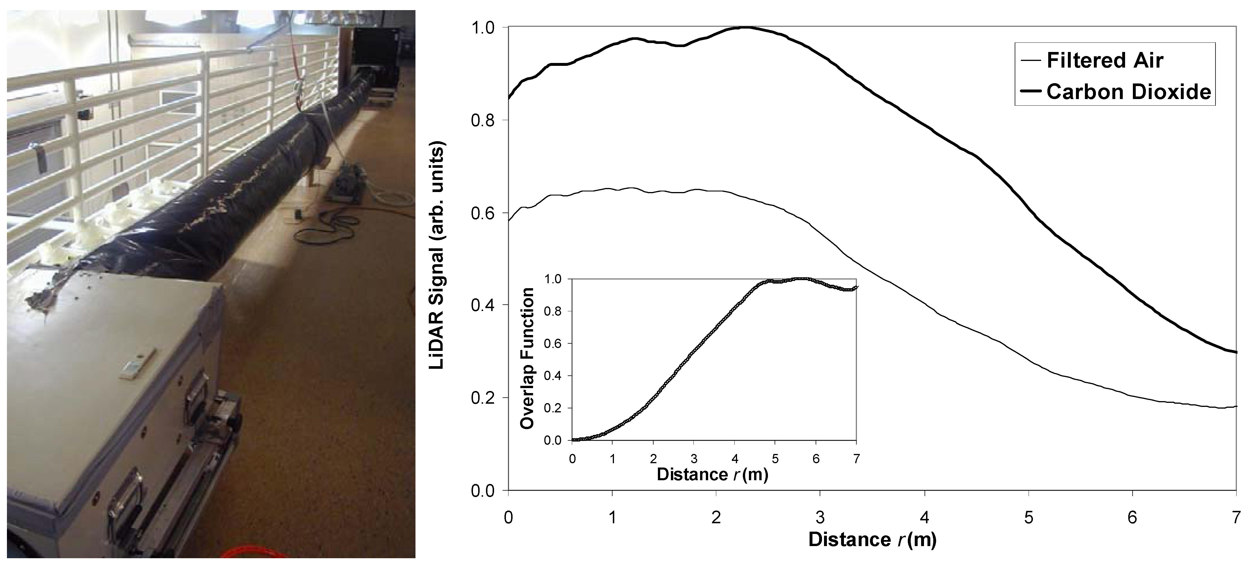
3.1.2. UV LiDAR and Transmissometer Unit

The UV LiDAR and transmissometer system described here was developed at the Desert Research Institute in Reno, Nevada, USA starting in 1999 and has been evolving and improving since then [11]. A typical field set-up is shown in Figure 1. All system components are transported to the site in a trailer that also serves as a heated/air-conditioned control room. For operation, the trailer is parked at the side of a road with single-lane traffic. The commercial unit to measure gaseous column contents is also deployed on the road. The main LiDAR and transmissometer units and the main gaseous units, containing the light sources and the detectors, are deployed next to the trailer, while the retro units, containing only passive components (mirrors and retro-reflectors), are deployed on the opposite side of the road, as shown in Figure 1. The height of the light beam is chosen to maximize the overlap between the beam and the probable location of the plume for the vehicle of interest (e.g., the light beam will be higher when sampling buses than for passenger vehicles).

Figure 1. Diagram (a) and picture (b) of a typical field set-up system of the PM LiDAR and gaseous measurement systems. The main unit contains all the light sources and detectors, while the retro unit incorporates a set of mirrors and retro-reflectors. A trailer hosting the data acquisition and computer system is parked on the side of a single-lane road where the exhaust plume of vehicles passing by is intercepted by the light beams.

Figure 1. Diagram (a) and picture (b) of a typical field set-up system of the PM LiDAR and gaseous measurement systems. The main unit contains all the light sources and detectors, while the retro unit incorporates a set of mirrors and retro-reflectors. A trailer hosting the data acquisition and computer system is parked on the side of a single-lane road where the exhaust plume of vehicles passing by is intercepted by the light beams.

The LiDAR UV transmitter utilizes a frequency-quadrupled, passively Q-switched Nd:YAG laser (Uniphase PowerChip NanoLaser PNU-001025-040) as a high-repetition rate (~1 kHz) source of sub-nanosecond, 266-nm pulses (with an energy of ~10 μJ per pulse). An internal photodiode generates a trigger signal for the data acquisition. The laser beam is directed across the road toward the retro unit. In the retro unit, two UV mirrors reflect the beam back, with a separation of ~27 cm from the outgoing beam, to the UV transmissometer receiver also located in the main unit. The UV transmissometer receiver measures the incident laser power with a large area photodiode operating in photovoltaic mode (UDT Sensor, Inc. UV-100 with a Corion G10-265-F band-pass filter mounted in front of it) and using a ~7.6-cm diameter UV fused silica lens that focuses the beam onto the photodiode. Its signal is processed by an analog gated integrator and digitized for further processing into a transmission or opacity reading.

The UV LiDAR receiver is located, in a biaxial arrangement, next to the outgoing UV beam. A 15-cm diameter spherical mirror collects the light backscattered by the particles suspended along the laser beam path, at ~180 degree and focuses it onto a fast, solar-blind photomultiplier tube (PMT) (Hamamatsu R7400U-06 with a quantum efficiency of ~28% @ 266 nm). A band-pass filter (Corion G10-265-F) is mounted in front of the PMT to reduce the contribution of background radiation. The PMT generates a negative current, which is a function of the incident optical power. It is necessary to operate the LiDAR system with a fast data acquisition system that allows the backscattering coefficient and consequently the PM concentration, to be measured as a function of range (i.e., distance from the main unit along the beam path). This is essential to (a) discriminate against the large signal from the retro unit, (b) correct for the 1/r² dependence of the collected backscattering signal and for the overlap function between beam path and field of view of the telescope resulting in range-independent sensitivity (also see the calibration procedure described below), and (c) make it possible to determine the spatial distribution of PM concentration along the beam path. A high bandwidth (i.e., 1.5 GHz with a 4 GSa/s sampling rate) digital oscilloscope measures the PMT current on a 50 Ω load, yielding a time-dependent waveform for each laser pulse.

This time-dependent waveform is converted to a distance-dependent waveform by multiplication of the time with one half the speed of light to account for the roundtrip of the UV radiation. The result is the LiDAR backscattering signal as a function of distance or range. As the UV wavelength of 266 nm is in the solar blind spectral region, the system can be operated in full sunlight without interference from solar background light. Figure 2 shows a schematic and a picture of the main unit.

Figure 2. Diagram and picture of the main unit of the UV LiDAR/transmissometer system.

Figure 2. Diagram and picture of the main unit of the UV LiDAR/transmissometer system.

The diagram includes two IR optical gates encompassing the laser beam in its horizontal and vertical extension. The two gates are connected to a fast (~1 ms opening/closing time) horizontal blade mechanical shutter in front of the laser. The two gates are kept activated (implying the mechanical shutter is open) only when their IR beam from the main unit to the retro unit is free of obstacles, by means of two plastic corner-cube type retro-reflectors on the other side of the road. If anything interrupts the optical circuit, the shutter is immediately closed. The reason for the shutter system is threefold: (1) Eye safety. Should anybody attempt to look into the beam, one or both of the optical gates would be interrupted and the shutter closed, avoiding any exposure; this is also true for reflected or diffused light from an object inserted in the path. (2) PMT protection. When a vehicle is passing through the beam, in absence of a shutter system, a large amount of UV light could be directly reflected into the main mirror and focused onto the PMT, potentially causing damage. (3) Measurement timing. The signal from the gate is used as a timing trigger for the measurement providing a reference with respect to the vehicle passage.

The acquisition system and data transfer for the experiments described here worked at a frequency of about 0.5 kHz, although commercially available acquisition cards are now able to sample each laser pulse at pulse repetition rates up to ~1 kHz. Data for ~300 milliseconds are continuously stored in a circular buffer. When a blocking trigger signal (a vehicle is passing through and is blocking the beam) is detected, the upstream optical gate sends a TTL signal to the computer. The buffering is then stopped and only the last 200 milliseconds of data are retained. These data are collected immediately before the vehicle passes and are used to estimate the background backscattering and extinction signals. These data represent the signal due to aerosols and gases that would be in the optical path in the absence of the vehicle under investigation. The data collected while the laser beam is blocked by the shutter, during vehicle passage, is used as an internal check to evaluate the “dark” noise background on the PMT and the UV-enhanced silicon photodiode. When the downstream optical gate is unblocked the laser shutter is opened and the vehicle data acquisition records the signals associated with the background plus the exhaust plume. Backscattering LiDAR returns are acquired for 500 milliseconds and associated, together with the pre-vehicle 200 milliseconds data, with the individual vehicle identification number. For each vehicle a synchronous picture is also taken by means of a digital camera. The vehicle PM mass concentration along the path and the column content are calculated by subtracting the pre-vehicle averaged signal from each post-vehicle LiDAR return and by calculating the excess backscattering and extinction in the optical path.

3.1.3. Method

a. Transmissometer

The UV transmissometer measures the power of the laser beam returning to the main unit after two passes through the exhaust plume (i.e., round trip from main unit to retro unit) as background-corrected photodiode signal (S_T) directly yielding the excess two-way opacity (OP₂) and relative two-way transmission (TR₂) as

$$O{P}_2=1-T{R}_2=1-\frac{S_T}{S_{T0}}$$

(5)

where S_T0 is the photodiode signal measured before the vehicle passes the sensor. The corresponding one-way excess optical depth τ (i.e., the optical depth added by the exhaust plume) between main unit and retro unit is expressed as

$$\tau =\frac{1}{2}\ln \left(\frac{1}{T{R}_2}\right)=\frac{1}{2}\ln \left(\frac{1}{1-O{P}_2}\right)$$

(6)

The excess optical depth τ is the relevant optical parameter measured by the transmissometer, and is converted to an excess PM mass column content (ρ_{c_PM}) by

$${\rho }_{c-PM}=\frac{\tau }{E_{ext}}=\frac{1}{2E_{ext}}\ln \left(\frac{1}{1-O{P}_2}\right)$$

(7)

when the mass extinction efficiency (E_ext) (dimension of area/mass) for the exhaust PM is known.

The E_ext for PM emitted by diesel and gasoline vehicles and for freshly entrained road dust is calculated in Section 3.2, as function of several assumptions. The relative range of E_ext values for reasonable changes in assumptions is ~10–20%. Therefore, the UV transmissometer gives a direct measurement of the excess PM mass column content especially suited for the measurement of optically dense plumes. This measurement is used to calculate the fuel-based PM EFs in conjunction with the excess carbon mass column content obtained from gaseous measurements. Road dust entrained by the vehicles from paved roads does not contribute significantly to the transmissometer signal at this wavelength due to its relatively low mass column content and because its much larger average diameter yields a low extinction efficiency. Theoretical calculations demonstrating that dust has a negligible contribution in typical paved-road conditions are presented in Section 3.2.

b. LiDAR Calibration and Inversion

In contrast to the transmissometer, the LiDAR needs to be calibrated to yield the backscattering coefficients in the beam path. When the PMT response is linear with the incident radiation, the signal S_L is given by the LiDAR equation as a function of the range (r) from the LiDAR system and can be written as:

$$S_L(r)=C_0\frac{O(r)}{r^2}\beta (r)T_2(r)=C(r)\beta (r)T_2(r)$$

(8)

where C₀ is the LiDAR constant including parameters such as laser pulse power, telescope area, PMT sensitivity, transmission of optical elements, etc.; O(r) is the overlap correction, which accounts for the geometric overlap of the field of view of the telescope and the laser beam and spatial variations of the PMT sensitivity [52]; 1/r² accounts for the acceptance solid angle of the receiver aperture; β(r) is the backscattering coefficient (dimension of 1/(length times spatial angle)); and T₂(r) is the two-way transmission between LiDAR system and range r [53]. The unknown coefficients O(r) and C₀ have been joined with 1/r² into the coefficient C(r), which must be determined through experimental calibration.

We should point out that Equation (8) is an approximation valid only for cases where the system temporal resolution (and therefore the range resolution) is much lower than the laser time pulse-width (the laser pulse is treated as a delta Dirac function). In our system however, the detection resolution (~1 ns) is comparable to the temporal pulse-width of the laser (~1 ns) and therefore a convolution with the laser temporal pulse shape should be included to provide a corrected version of the lidar equation (for a full treatment see Chapter 7 in Measures [53]). In our application though, we are interested in the PM emission factors and in the current system these are calculated by integrating the backscattering signals over the entire column to be compared with the column-content measurements of CO₂, CO, and HC. In this case, the resolution (i.e., the entire width of the road and some more) is considerably larger than the laser pulse-width making a correction unnecessary.

For most LiDAR systems, experimental calibration is limited as typical maximum ranges vary from 1 km to over 100 km, and calibration cells enclosing the entire range are impractical; although some novel LiDAR systems have a range close to 100–200 m (e.g., [54,55]). In our application, however, the LiDAR is used over a typical range of just 5–7 m and therefore a calibration can be easily performed in the laboratory; a ~8 m-long, ~50 cm-diameter calibration cylindrical plastic bag is attached to the enclosure of the main unit and terminates the beam with a beam dump (see picture in Figure 3). This cell can be completely evacuated (the bag collapses if air is removed with a pump) and then filled with calibration gases having different, well-known backscattering coefficients. The LiDAR system can be calibrated as a function of r yielding the calibration coefficient, C(r). Examples of calibration signals from HEPA-filtered air (β_air is 27 Mm⁻¹sr⁻¹ at standard pressure and temperature) and CO₂ (β_CO2 is 70 Mm⁻¹sr⁻¹ at standard pressure and temperature) are shown in Figure 3. From the figure and the insert it is possible to appreciate that the overlap correction function O(r) for this LiDAR is such that in the near field, 2–4 m range from the main unit, the signal is almost constant with r. This is primarily due to the limited overlap of the laser beam with the field of view of the mirror, but also due to the “shadow” that the rectangular case of the PMT casts on the collecting mirror, especially in the near field. This peculiar range-dependence is useful because it reduced the severity of the range correction needed and it is therefore less sensitive to errors or variability in the range correction function; it also reduces the needed dynamic range for the data acquisition system.

Figure 3. Picture of the calibration procedure and examples of data of the resulting LiDAR returns for filtered air and CO₂. The insert reports the calculated overlap function.

Figure 3. Picture of the calibration procedure and examples of data of the resulting LiDAR returns for filtered air and CO₂. The insert reports the calculated overlap function.

Once calibrated, the system can be used to determine the backscattering coefficient β(r) as

$$\beta (r)=\frac{1}{T_2(r)}\frac{S_L(r)}{C(r)}=\frac{1}{{\left[\exp \left(-{\displaystyle {\int }_{r_M}^r\sigma (r)dr}\right)\right]}^2}\frac{S_L(r)}{C(r)}$$

(9)

where σ(r) is the extinction coefficient. In most cases T₂(r) is close to 1. However, as mentioned above, one of the advantages of the system presented here is that the total transmission is also measured. When the extinction of the laser beam is above a certain threshold (e.g., for optically think plumes with T < 0.9), a Kunz’s [56] LiDAR inversion algorithm is applied to retrieve the correct backscattering coefficient by first calculating the range dependent extinction and then substituting into (9):

$$\sigma (r)=\frac{1}{2}\frac{S_L(r)/C(r)}{\frac{{\displaystyle {\int }_{r_M}^{r_R}{S}_L(r)/C(r)dr}}{(1-T_2)}-{\displaystyle {\int }_{r_M}^r{S}_L(r)/C(r)dr}}$$

(10)

where T₂ in this case represents the measured total transmission over the path between the main unit at position r_M and the retro unit at r_R and back.

The LiDAR measures the backscattering coefficient β(r) before (β₀(r)) and after (β₁(r)) the vehicle passes, yielding the excess backscattering coefficient β_E(r) as β_E(r) = β₁(r) − β₀(r). The β_E(r) is the relevant parameter measured by the UV LiDAR, and it can be converted to an excess range-dependent PM mass concentration ρ(r) using a mass backscattering efficiency [E_bscat; dimension of area/(mass times spatial angle)] that depends on aerosol optical and physical properties. A theoretical calculation of the E_bscat is described in Section 3.2. Figure 4 shows an example of the PM mass concentration measured in time immediately after an emitting vehicle passed through the laser beam.

Figure 4. Gasoline vehicle passing through the LiDAR system (the license plate has been obscured for privacy reasons) deployed near Boise, Idaho, USA in winter 2004. On the right panel the excess PM mass concentrations emitted by the gasoline vehicle are represented in an intensity chart. The concentrations were calculated from the LiDAR returns after correcting for the non-linearity of the detector. Range- and extinction-corrections have been applied after the background signal has been subtracted. No correction has been applied to account for the finite temporal pulse width of the laser. The abscissa axis represents the time (in milliseconds) elapsed after the vehicle passed through the system. The ordinate axis represents the distance across the road r from the main unit (in meters). The color scale represents the PM mass concentration (in µg/m³) with white being the highest concentration; evident is the plume dispersion.

Figure 4. Gasoline vehicle passing through the LiDAR system (the license plate has been obscured for privacy reasons) deployed near Boise, Idaho, USA in winter 2004. On the right panel the excess PM mass concentrations emitted by the gasoline vehicle are represented in an intensity chart. The concentrations were calculated from the LiDAR returns after correcting for the non-linearity of the detector. Range- and extinction-corrections have been applied after the background signal has been subtracted. No correction has been applied to account for the finite temporal pulse width of the laser. The abscissa axis represents the time (in milliseconds) elapsed after the vehicle passed through the system. The ordinate axis represents the distance across the road r from the main unit (in meters). The color scale represents the PM mass concentration (in µg/m³) with white being the highest concentration; evident is the plume dispersion.

The PM column content ρ_{c_PM} can be obtained by integrating ρ across the exhaust plume. As the exact location of the exhaust plume is generally not known (the tailpipe may be on the left or on the right side of the vehicle), a conservative procedure integrates over all of the useful LiDAR range from r_M to r_R, yielding ρ_{c_PM} as

$${\rho }_{c\_PM}={\displaystyle {\int }_{r_M}^{r_R}\rho (r)dr}=\frac{1}{E_{bscat}}{\displaystyle {\int }_{r_M}^{r_R}{\beta }_E(r)dr}$$

(12)

In summary, ρ_{c_PM} (i.e., the mass column content after passage of the vehicle minus the mass column content before passage of the vehicle) can be directly calculated from the measured excess UV LiDAR signal using E_bscat. Therefore, the UV LiDAR gives, after calibration, a direct and sensitive measurement of the excess PM mass column content. This is used to calculate the fuel-based PM EF in conjunction with the excess carbon mass column content obtained from gaseous VERSS measurements also deployed in the field. Contributions to the UV LiDAR signal from road dust entrained by the vehicle on paved roads is typically negligible due to its relatively low concentration and its lack of correlation with the excess carbon mass column content. A more detailed theoretical discussion of the dust contribution to extinction and backscattering is presented in Section 3.2.

c. Linearity and Dynamic Range Limitations of the Detector

The equations discussed above are valid only if the PMT is linear with respect to the incident radiation (the radiation backscattered by the particles and collected by the mirror). In reality, the PMT behaves non-linearly at high signals. In pulsed mode, as it is the case for a typical LiDAR, there are two main identified causes, which are responsible for PMTs nonlinearities:

(1) Space charge limitations at the last few dynodes.

(2) Radial voltage drop at the photocathode caused by the large current densities.

The first is recognized as the main PMT linearity limitation especially at large gain conditions (the gain is adjustable by changing the control voltage (CV) applied to the PMT module). Additionally, it has been reported that temperature may have a strong effect on the PMT signal especially in non-linear regime [57]. The behavior of the PMT used in the PM VERSS was characterized by measuring LiDAR returns from a hard target in the laboratory for different CVs (i.e., gains) and a set of calibrated neutral density optical filters.

For an application such as that described here, where thousands of vehicle data are analyzed and processed in a short time, a simple empirical model needs to effectively correct the PMT nonlinearity. Linear behavior is expected at low incident intensities, whereas at a high power complete saturation is observed. A hyperbolic curve was chosen as a simple analytical function to describe the signal from low power to saturation:

$$S_{L\_meas}(r)=\frac{S_{L\_PMT}(r)\cdot P_1}{P_2(r)+S_{L\_PMT}(r)}$$

(11)

where S_{L_meas} is the measured LiDAR return and S_{L_PMT} is the intensity of the signal that would be measured by a linear detector. The two parameters P₁ and P₂(r) represent the saturation level (independent of r) and a scaling factor (range dependent). For small signals, the response is linear with slope C(r) = P₁/P₂(r), where C(r) is the range correction factor used in the analysis above. For large signals however the response tends to a saturation level represented by P₁. This empirical formula fits the extensive data collected in the laboratory at the typical working conditions found in the field.

The experimental procedure to measure P₁ and P₂(r) consists of measuring the LiDAR signal using a hard target at different distances and using calibrated neutral density filters in front of the detector (with transmission ranging from ~0.0002 to 1) to attenuate the signal reaching the PMT. The values for P₁ and P₂(r) that best fit the experimental data depend on the chosen CV and the laser power. The system was tested for a variety of CV values from 0.3 to the maximum 0.8 V, encompassing the typical working conditions used in the field. In Figure 5 we report the result of such study and the typical boundaries of the signals measured in the field (from minimum to maximum).

Figure 5. LiDAR returns from a hard target and using different neutral density filters versus the optical density of the filters. The plot shows different curves for different values of the voltage control (gain) of the photomultiplier. The shaded box represents typical working conditions in the filed from the minimum to the maximum signals.

Figure 5. LiDAR returns from a hard target and using different neutral density filters versus the optical density of the filters. The plot shows different curves for different values of the voltage control (gain) of the photomultiplier. The shaded box represents typical working conditions in the filed from the minimum to the maximum signals.

The choice of CV determines the level of saturation at high signals. A high saturation signal (meaning reaching saturation only at very large incident light levels) implies a higher linearity of the detector and therefore a more straightforward and less error-prone calibration. A low saturation signal (meaning saturation is reached at low incident intensities) implies a strong nonlinearity. However, the low saturation signal also implies that for a specified scale and for a given resolution on the scope acquiring the data, the signal dynamic range can be significantly increased because the signal is “compressed” between the linear regime and the saturation level. An optimal choice of CV represents a trade-off between linearity and dynamic range. To establish the best working conditions (the best choice for CV and laser power), one needs to consider the dynamic range that is typically needed in the field (assuming that only one acquisition channel is available, as it is the case for this system) and the errors introduced by the nonlinearity of the detector. A detailed error and error propagation analysis was performed to establish the best compromise between sensitivity and dynamic range considering the laser power and the detection linearity.

d. Source of Uncertainty

The following sources of noise and limitations were considered: (1) uncertainties in the fit parameters and drifts with ambient conditions (in particular the saturation value is temperature dependent), (2) photo-electron noise, (3) digitization error introduced by the limited bit resolution of the scope, (4) limited throughput of the data acquisition and storage system (software and hardware), (5) laser availability. A direct measurement of the saturation level is performed in the field by monitoring the fully saturating signal from scattered UV-light by dust deposited on, and imperfections in the optics at the retro-unit. These data are used to evaluate the variability of the saturation level at a given CV. We also estimated the typical signals from vehicles that need to be measured in the field, ranging from low emitting gasoline passenger vehicles to high emitting diesel trucks and buses based on field data collected near Boise, Idaho in 2004. A PM VERSS needs to have high sensitivity (implying powerful laser and fast acquisition system) and a large dynamic range to be able to measure all the vehicles between these two extremes. Considering the acquisition system specifications, a laser pulse power of ~10 μJ/ns, a CV of 0.7±0.1 V was found to be an optimal choice to minimize the errors (estimated to be less then 10%) while maintaining the dynamic range necessary for this application. The data analyzed were therefore corrected for the nonlinearity of the detection system by using the saturations signals measured directly in the field at a given CV (typically 0.7–0.8 V).

In addition to the sources of uncertainties discussed above, there is also a possible source of positive bias due to the gaseous molecular backscattering present in the vehicle plume. The molecular backscattering of background gases (i.e., air) is subtracted out during the emission factor calculation as described above and therefore does not contribute to the measured PM emission factor. However, there is an additional contribution to molecular backscattering due to the fact that the combustion process replaces some of the molecular oxygen in the atmosphere with added carbon dioxide (with a 266-nm backscattering efficiency about three times higher than molecular oxygen) and water. A calculation assuming a worst case scenario of perfectly stoichiometric combustion shows that the added backscattering signal due to carbon dioxide and water in the plume would correspond to an equivalent PM emission factor of just ~0.5 mg/Kg_Fuel. Considering that average PM emission factors for spark ignition vehicles is in the order of 50 mg/kg_Fuel [14], and considering that, as described in more detailed later on, the minimum detection limit for a single vehicle for the more sensitive LiDAR system described here is ~60 mg/kg_Fuel, it is evident that the added molecular scattering contributes less than 1%, and is therefore negligible in a practical application.

e. Gaseous Remote Sensing Unit

As mentioned in Section 2 the calculation of PM emission factors relies on the normalization of the PM mass column content to the total carbon column content. A commercial path integrated CO₂, CO, and HC unit is therefore used in conjunction with the PM VERSS. This unit also measures the NO column content (ESPI RSD3000, Phoenix, AZ, USA). The gaseous system is based on a broadband extinction measurement by using IR and UV radiation sources [58]. As the gaseous absorption is a strong function of wavelength within the wavelength bands detected, Beer-Lambert law does not apply because individual absorption bands have different exponential constant and the sum of exponentials with different constants is not an exponential. In short, the Beer-Lambert law does not apply if there is spectral, spatial, or temporal in-homogeneity within the generalized (multi-dimensional) measurement volume. Therefore, the received signals must be calibrated as a function of CO₂, CO, HC, and NO mass column contents. For this purpose a known mixture of CO₂, CO, HC, and NO is dispersed in air in front of the main unit at regular intervals. Measuring the electric signals as a function of gases mass column content produces individual gas calibration curves. An example of PM emission factor calculation is presented in Section 3.3 [46].

3.2. Backscattering and Extinction Mass Efficiencies: Theoretical Approach

3.2.1. Particulate Matter Extinction Mass Efficiency

It was shown in Section 3.1 that the relevant parameters measured by the transmissometer and the LiDAR are the excess two-way transmission (TR₂) and the excess backscattering coefficient (β_E(r)) [12]. The two-way transmission (TR₂) is related to the total number of particles N_PM present in the volume sampled by the laser along the optical path, their size distribution function ${\overline{n}}_N(D)$ (with $N_{PM}{\overline{n}}_N(D)dD$ representing the number concentration of particles with diameter between D and D + dD) and their extinction cross section ${\sigma }_{e,PM}(D)$:

$$T{R}_2=\frac{I_{2L}}{I_0}=\exp \left(-2L{N}_{PM}{\displaystyle {\int }_0^{\infty }{\sigma }_{e.PM}(D){\overline{n}}_N(D)dD}\right)$$

(13)

where L is the distance between the laser source and the retroreflector on the opposite side of the road. The factor of 2 accounts for the roundtrip path, since the beam is reflected back to the detector in the main unit. The main regulatory interest, however, is focused on PM mass, that is related to the number concentration as

$$\rho =N_{PM}\langle m_{PM}\rangle =\frac{1}{2L}\ln \frac{1}{T{R}_2}\frac{{\displaystyle {\int }_0^{\infty }{m}_{PM}(D){\overline{n}}_N(D)dD}}{{\displaystyle {\int }_0^{\infty }{\sigma }_{e.PM}(D){\overline{n}}_N(D)dD}}=\frac{1}{2L}\ln \frac{1}{T{R}_2}\frac{\eta {\displaystyle {\int }_0^{\infty }V(D){\overline{n}}_N(D)dD}}{{\displaystyle {\int }_0^{\infty }{\sigma }_{e.PM}(D){\overline{n}}_N(D)dD}}$$

(14)

where V(D) is the volume of a particle with diameter D (V(D)= D³π/6 for a spherical particle), and η is the bulk particle density. Therefore

$$\rho =\frac{1}{E_{ext}2L}\ln \left(\frac{1}{T{R}_2}\right)$$

(15)

where E_ext is the mass extinction efficiency:

$$E_{ext}=\frac{{\displaystyle {\int }_0^{\infty }{\sigma }_{e.PM}(D){\overline{n}}_N(D)dD}}{\eta {\displaystyle {\int }_0^{\infty }V(D){\overline{n}}_N(D)dD}}$$

(16)

The implicit assumptions here are that the particle characteristics are the same along the optical path and that η is independent on the particle size. The first assumption is a reasonable approximation if we consider that the sampling is done perpendicularly to the vehicle plume and the source of the PM is an individual vehicle under a specific load (the measurement is almost instantaneous). The assumption that η is independent with size is reasonable because the values used for η are averages over different size distributions.

3.2.2. Particulate Matter Backscattering Mass Efficiency

A similar derivation applies to the LiDAR measurement with the exception that (a) at this point, the particle concentration is not integrated over the optical path, due to the fact that the backscattering signal depends on the distance r (the particle concentration is not uniform across the road), and (b) the extinction cross section needs to be substituted with the averaged differential backscattering cross section (σ_d,PM(π,D)):

$${\beta }_{PM}(r)=N_{PM}(r){\displaystyle {\int }_0^{\infty }{\sigma }_{d,PM}(\pi ,D)}{\overline{n}}_N(D)dD$$

(17)

Here, the assumption was made that the plume is uniformly mixed, implying that we neglect any dependency of ${\overline{n}}_N(D)$ and ${\sigma }_{d,PM}(\pi ,D)$ with the range r. This assumption is reasonable if we consider that the only source of PM in excess of the background PM is due to each individual vehicle, and considering that the measurement is completed in a very short time (0.5 seconds), implying stationary vehicle load conditions and short PM aging time.

Therefore, an expression for the PM concentration at range r is:

$$\rho (r)={\beta }_{PM}(r)\frac{\eta {\displaystyle {\int }_0^{\infty }V(D){\overline{n}}_N(D)dD}}{{\displaystyle {\int }_0^{\infty }{\sigma }_{d.PM}(\pi ,D){\overline{n}}_N(D)dD}}={\beta }_{PM}(r)/E_{bscat}$$

(18)

where E_bscat is the PM backscattering mass efficiency

$$E_{bscat}=\frac{{\displaystyle {\int }_0^{\infty }{\sigma }_{d.PM}(\pi ,D){\overline{n}}_N(D)dD}}{\eta {\displaystyle {\int }_0^{\infty }V(D){\overline{n}}_N(D)dD}}$$

(19)

Typically (to calculate EFs by normalizing with the CO₂ column content), ρ(r) is integrated across the roadway to give an excess (after vehicle minus before vehicle) PM concentration column density with units of gm⁻². The quantities that enable transmission and backscattering measurements to be converted to PM mass concentration are the efficiencies given by (16) and (19), respectively. Numerical evaluation requires that certain assumptions be made about particle morphology and composition as well as the size distributions of exhaust PM.

3.2.3. Applications to Vehicle Emitted Particulate

Studies of particle morphology using electron microscopes have shown that individual particles emitted from diesel and spark-ignition engines exhibit fractal-like characteristics [59,60]. However, specific parameters of the fractal-like particles, such as fractal dimension and radius of gyration, are widely variable dependent upon engine type (spark-ignition or diesel) and operating characteristics, as well as on the specific conditions that exist at the time of measurement [61,62,63,64].

Despite these complexities, there is an immense literature of exhaust particle measurements that present particle sizes and size distributions in terms of equivalent spheres. For example, differential mobility analyzer/condensation nucleus counters measure particle electrical mobility and assume that particles are spherical in shape to infer particle size [65,66,67,68,69,70,71,72,73]. Similarly, optical particle counters are calibrated with aerosols composed of spherical particles and present results in terms of these calibrated particles. Cascade impactors measure particle aerodynamic diameter that is then converted to particle physical diameter by assuming that particles are spherical in shape, although often this is not the case for freshly emitted soot particles [60,74].

Additional ambiguity exists in defining other characteristics of exhaust particles, although some generalizations are possible. Spark-ignition exhaust particle volume consists largely of organic material, while diesel exhaust particles contain widely varying volume fractions of elemental carbon (EC) and organic carbon. Particle mass size distributions may be approximated as log-normal with a mass median diameter of about 0.15 μm and a geometric standard deviation of 1.5 for both spark-ignition and diesel engines (there is evidence that the peak diameter of the particle mass distribution for spark-ignition engines is less than that for diesel engines [73,75,76]). Particle bulk density η is found to range from 1.0 to 1.5 g cm⁻³ (1.25 g cm⁻³ is used here).

Knowledge of the complex index of refraction of carbon compounds, m = n − ik, is required to calculate light scattering and absorption properties of the exhaust particles. EC is highly absorbing and an index of refraction m = 1.5 − i0.5 appears to be a reasonable value at ultraviolet wavelengths and for the bulk density chosen here [77]. We assume here that the organic material in vehicle exhaust can be represented by a real index of refraction, m = 1.5, i.e., the organic material is assumed to be nonabsorbing.

As an example of obtaining numerical values for (16) and (19), we assume the equivalent sphere particle models and size distributions that result from exhaust particle measurements using contemporary instrumentation. The adoption of this simple model also permits a systematic study of (16) and (19) to parametric changes in the assumed particle characteristics.

With the previously defined mass size distributions and particle density, numerical evaluation for spark-ignition vehicles (solid particle with m = 1.5) and diesel vehicles (equivolume two-layer core-shell particle: core with m = 1.5 − i0.5 and shell with m = 1.5) gives the values reported in table 1.

Table 1. Theoretical extinction and backscattering PM mass efficiencies for different engine types.

	Eext (m2g−1)	Ebscat (m2g−1sr−1)	LR = Eext/Ebscat (sr)
Spark-ignition	10	0.16	63
Diesel	13	0.08	163

Table 1. Theoretical extinction and backscattering PM mass efficiencies for different engine types.

	Eext (m2g−1)	Ebscat (m2g−1sr−1)	LR = Eext/Ebscat (sr)
Spark-ignition	10	0.16	63
Diesel	13	0.08	163

Table 1 also reports the two values of the LiDAR ratio (LR) for spark-ignition and diesel vehicles. The LiDAR ratio for diesel PM is larger than that for spark-ignition PM by a factor of about 2.6. If simultaneous LiDAR and transmissometer measurements are made, calculation of the LiDAR ratio can be used to distinguish between diesel and spark-ignition vehicles, or more generally between vehicles emitting black and white exhaust plumes.

3.2.4 Mass Efficiency Sensitivity Study

The degree of sensitivity of the calculated quantities to changes in the assumed particle characteristics can be assessed by varying the characteristics systematically.

a. Particle Density

The bulk density η appearing in (16) and (19) is a multiplicative constant, so the calculated quantities in Table 1 will vary directly with η, i.e., a 10% change in η will result in a 10% change in the calculated mass efficiencies. Other parameters that can be varied to determine their influence on the calculated mass efficiencies are the index of refraction used to calculate the cross section quantities and the mass median diameter and geometric standard deviation of the particle size distribution. These sensitivities are explored separately for the spark-ignition and diesel cases.

b. Spark-Ignition Vehicle Emissions

The sensitivity study examines varying the real index of refraction as well as including an imaginary component to simulate an absorbing PM particle. We also examine the effect of using a mass median diameter of 0.15 μm ± 0.025 μm and a geometric standard deviation of 1.5 ± 0.25. Table 2 shows the results of the sensitivity testing for the spark-ignition case. Rows 1–3 show that E_bscat and E_ext are quite sensitive to variations in the real index of refraction m. A 3% change in m results in an approximate 20% proportionate change in backscattering and extinction mass efficiencies. Rows 4 and 5 show that including an imaginary component in the index of refraction to simulate an absorbing PM particle causes E_bscat to decrease markedly and E_ext to increase slightly. Rows 6–11 show that a 17% change in either the mass median diameter (rows 6–8) or geometric standard deviation (rows 9–11) results, on average, in similar percentage changes in the mass efficiencies. The sensitivities of E_ext to changes in the mass median diameter and E_bscat to changes in the geometric standard deviation are more pronounced.

Table 2. Sensitivity of calculated mass efficiencies: spark-ignition vehicles.

m	Dgm	σg	Ebscat	Eext
1.45	0.15	1.5	0.13 (−19%)	8.1 (−19%)
1.5	0.15	1.5	0.16	10
1.55	0.15	1.5	0.20 (+25%)	12 (+20%)
1.5-i0.05	0.15	1.5	0.11 (−31%)	11 (+10%)
1.5	0.125	1.5	0.16 (0%)	7.8 (−22%)
1.5	0.175	1.5	0.18 (+12%)	11 (+10%)
1.5	0.15	1.25	0.13 (−19%)	10 (0%)
1.5	0.15	1.75	0.18 (+12%)	9.2 (−8%)

• Values used for the emission factor calculations are shown in bold
• m = index of refraction
• D_gm = mass median diameter
• σ_g = geometric standard deviation

Table 2. Sensitivity of calculated mass efficiencies: spark-ignition vehicles.

m	Dgm	σg	Ebscat	Eext
1.45	0.15	1.5	0.13 (−19%)	8.1 (−19%)
1.5	0.15	1.5	0.16	10
1.55	0.15	1.5	0.20 (+25%)	12 (+20%)
1.5-i0.05	0.15	1.5	0.11 (−31%)	11 (+10%)
1.5	0.125	1.5	0.16 (0%)	7.8 (−22%)
1.5	0.175	1.5	0.18 (+12%)	11 (+10%)
1.5	0.15	1.25	0.13 (−19%)	10 (0%)
1.5	0.15	1.75	0.18 (+12%)	9.2 (−8%)

• Values used for the emission factor calculations are shown in bold
• m = index of refraction
• D_gm = mass median diameter
• σ_g = geometric standard deviation

c. Diesel Vehicle Emissions

The diesel mass backscattering and extinction efficiencies can be found in the literature [59,78]. The sensitivity study examines varying the real and imaginary parts of the index of refraction. We also examine the effect of varying the mass median diameter and the geometric standard deviation as for the spark ignition case as well as varying the volume fraction of elemental carbon to organic carbon (EC/OC). Table 3 shows the result of the sensitivity testing for the diesel case. Rows 1–3 vary m in the shell while rows 4–5 vary the real part of m in the core. Rows 1–5 show that E_bscat and E_ext are relatively insensitive to changes in m. Rows 6–7 show that changing the volume fraction EC/OC also has little influence on the calculated mass efficiencies. Rows 8–11 show that E_bscat is quite sensitive to variations in the mass median diameter and the geometric standard deviation, even more so than for the spark-ignition case shown in rows 6–11 of Table 2. E_ext is insensitive to changes in the mass median diameter, while its sensitivity to the geometric standard deviation is similar to that observed for the spark-ignition case.

Table 3. Sensitivity of calculated mass efficiencies: diesel vehicles.

m (core, shell)	Fractional core:shell volume	Dgm	σg	Ebscat	Eext
(1.5-i0.5, 1.45)	0.5:0.5	0.15	1.5	0.08 (0%)	13 (0%)
(1.5-i0.5, 1.5)	0.5:0.5	0.15	1.5	0.08	13
(1.5-i0.5, 1.55)	0.5:0.5	0.15	1.5	0.08 (0%)	13 (0%)
(1.45-i0.5, 1.5)	0.5:0.5	0.15	1.5	0.08 (0%)	13 (0%)
(1.55-i0.5, 1.5)	0.5:0.5	0.15	1.5	0.09 (+12%)	14 (+8%)
(1.5-i0.5, 1.5)	0.4:0.6	0.15	1.5	0.09 (+12%)	12 (−8%)
(1.5-i0.5, 1.5)	0.6:0.4	0.15	1.5	0.08 (0%)	14 (+8%)
(1.5-i0.5, 1.5)	0.5:0.5	0.125	1.5	0.11 (+38%)	13 (0%)
(1.5-i0.5, 1.5)	0.5:0.5	0.175	1.5	0.06 (−25%)	13 (0%)
(1.5-i0.5, 1.5)	0.5:0.5	0.15	1.25	0.06 (−25%)	14 (+8%)
(1.5-i0.5, 1.5)	0.5:0.5	0.125	1.75	0.09 (+12%)	12 (−8%)

• Values used for the emission factor calculations are shown in bold
• m = index of refraction
• D_gm = mass median diameter
• σ_g = geometric standard deviation

Table 3. Sensitivity of calculated mass efficiencies: diesel vehicles.

m (core, shell)	Fractional core:shell volume	Dgm	σg	Ebscat	Eext
(1.5-i0.5, 1.45)	0.5:0.5	0.15	1.5	0.08 (0%)	13 (0%)
(1.5-i0.5, 1.5)	0.5:0.5	0.15	1.5	0.08	13
(1.5-i0.5, 1.55)	0.5:0.5	0.15	1.5	0.08 (0%)	13 (0%)
(1.45-i0.5, 1.5)	0.5:0.5	0.15	1.5	0.08 (0%)	13 (0%)
(1.55-i0.5, 1.5)	0.5:0.5	0.15	1.5	0.09 (+12%)	14 (+8%)
(1.5-i0.5, 1.5)	0.4:0.6	0.15	1.5	0.09 (+12%)	12 (−8%)
(1.5-i0.5, 1.5)	0.6:0.4	0.15	1.5	0.08 (0%)	14 (+8%)
(1.5-i0.5, 1.5)	0.5:0.5	0.125	1.5	0.11 (+38%)	13 (0%)
(1.5-i0.5, 1.5)	0.5:0.5	0.175	1.5	0.06 (−25%)	13 (0%)
(1.5-i0.5, 1.5)	0.5:0.5	0.15	1.25	0.06 (−25%)	14 (+8%)
(1.5-i0.5, 1.5)	0.5:0.5	0.125	1.75	0.09 (+12%)	12 (−8%)

• Values used for the emission factor calculations are shown in bold
• m = index of refraction
• D_gm = mass median diameter
• σ_g = geometric standard deviation

These tests demonstrate that the calculated mass efficiencies are moderately dependent upon variations in the assumed PM characteristics, more so for the spark-ignition case than the diesel case. It is likely that the presence of absorbing EC in diesel exhaust PM explains, in part, the relative insensitivity of the mass efficiencies upon the assumed PM characteristics. To the extent that spark-ignition exhaust PM also contains EC then the sensitivity displayed in Table 2 should decrease.

d. Road Dust Contribution

Road dust can be a potential contributor to the backscattering and opacity measurements and its effect needs to be quantified to understand the limitations of the system on roads with higher level of dust. Calculations of the average backscattering and opacity for dust particles and vehicle exhaust can provide an approximation of the influence of dust particles on the tailpipe measurements.

The average backscattering for vehicle exhaust at 266 nm is approximately 10⁻¹⁶ m² sr⁻¹ across the range of EC/OC volume fractions. Typical tailpipe number concentrations N range from 10¹¹ m⁻³ for spark-ignition vehicles [73,76,79] to 10¹⁴ m⁻³ for diesel vehicles [63,73,75] and will typically change with the distance from the emission. Therefore, the product N_PM(r)‹σ_d,PM(π)› for tailpipe emissions in (17) ranges from 10⁻⁵ m⁻¹sr⁻¹ to 10⁻² m⁻¹sr⁻¹ for spark-ignition and diesel vehicles, respectively.

A worst-case scenario considers dust concentrations existing immediately behind the vehicle tires. These measurements have been made for paved roads as a function of vehicle speed [80]. The dust concentration was sampled with an inlet positioned 17.5 cm above the roadway and 47 cm behind the axis of rotation of the tire. A typical number concentration for dust at a vehicle speed of 65 km h⁻¹ is N = 10⁷ m⁻³.

The calculated average backscattering at 266 nm for a lognormal distribution of dust particles with a mass median diameter of 4 μm and a geometric standard deviation of 2 is about 10⁻¹³ m² sr⁻¹. This value has been calculated using a Mie code and is therefore only an approximation used here to gain an estimation of the dust interference, because the shape of dust resuspended by vehicles is variable and generally unknown. The product of the number density and the average backscattering for dust particles is 10⁻⁶ m⁻¹sr⁻¹. This is one and four orders of magnitude below the corresponding product for spark-ignition and diesel vehicle exhaust, respectively. Since these dust measurements were made directly behind the tire, dilution of the dust number concentrations at the location of the vehicle exhaust plume reduces the product even further. In conclusion, the LiDAR return at 266 nm from dust on paved roads is typically negligible compared to that from vehicle exhaust.

The opacity for vehicle exhaust at 266 nm is approximately 0.9 across the range of EC/OC volume fractions. N, the number concentration, was assumed to be 10¹⁴ m⁻³, typical of diesel vehicles, for these calculations. Similar calculations for a number concentration of 10¹¹ m⁻³, typical of spark-ignition vehicles, give opacity of about 10⁻³. This example illustrates why opacity is difficult to measure for spark-ignition vehicles and why a backscattering measurement through a LiDAR approach is more sensitive.

Similar to the relative significance observed with backscattering, calculations for the log-normal distribution of dust particles described above give opacity of 10⁻⁴, one to four orders of magnitude below that for spark-ignition or diesel PM, respectively. Opacity at 266 nm from dust on paved roads is negligible compared to that from vehicle exhaust.

The mass efficiency factors at 266 nm for dust are E_bscat = 0.07 m² g⁻¹ sr⁻¹ and E_ext = 0.9 m² g⁻¹. This E_ext value is comparable to the scattering mass efficiency (E_scat = 0.4 m² g⁻¹ at 550 nm) used by Moosmüller et al. [81] for freshly entrained dust. The mass backscattering efficiency for dust is comparable to that for exhaust, given in Table 1. It is the greater mass concentration of vehicle exhaust that results in its larger LiDAR signal for exhaust PM. The mass extinction efficiency for dust is an order of magnitude less than that in Table 1.

From these calculations we can also determine that the LiDAR ratio (E_ext/ E_bscat) for dust is 13 sr to be compared to 163 sr for diesel PM and 63 sr for spark ignition PM as reported in Table 1. Typical values of the LiDAR ratio found in literature for atmospheric aerosol are lower than the value calculated here for diesel vehicles and are more similar to the value calculated here for gasoline vehicles [82,83,84]. This is reasonable considering that diesel particulates emitted at the tailpipe of the vehicle have a high fraction of small-sized and strongly absorbing particles (black carbon), enhancing extinction due to absorption with respect to backscattering; an increase of the LiDAR ratio with the enhancement of small absorbing aerosol concentrations in polluted airmasses has been measured before [85]. Particles commonly measured by LiDAR are often more aged; aging generally results in a “whitening” of black carbon particles and in an increase of size due to mixing, coagulation, coating, oxidation, humidification etc. [86]. In the contrary, the LiDAR ratio calculated here for dust is on the lower end of the typical ratios measured or calculated for atmospheric dust [84], although similar values have been estimated for atmospheric dust before [87]. The low value for the LiDAR ratio of dust resuspended by vehicles is probably due to the larger particle sizes close to the vehicle tires (mass median diameter of 4 μm). Such large particles settle out quickly and do not remain suspended in the atmosphere long enough to be measured in typical, longer range LiDAR applications [88]. We should also caution the reader that these calculations were done assuming spherical shape. The resuspended dust will significantly deviate from the perfectly spherical shape and this will probably result in a reduced backscattering efficiency, therefore increasing the LiDAR ratio; for this reason the dust LiDAR ratio reported here probably represents a lower limit. It should also be noticed that in a situation in which the LiDAR signal is dominated by vehicle-entrained road dust, which is possible for unpaved roads or if large amounts of silt have been deposited onto a paved road, the LiDAR ratio would clearly indicate this.

As mentioned previously, LiDAR and transmissometer excess PM measurements are obtained as an integrated and path-averaged result across the entire roadway, respectively, eliminating a dependence on variably positioned exhaust pipes. Measurements from dust are incorporated in the same integration and path-average approach as for the excess PM and therefore should not change the conclusion that the LiDAR return and the opacity from dust is negligible compared to that from vehicle exhaust. A field validation of the backscattering mass efficiency calculated on this theoretical basis is discussed in Section 3.4.

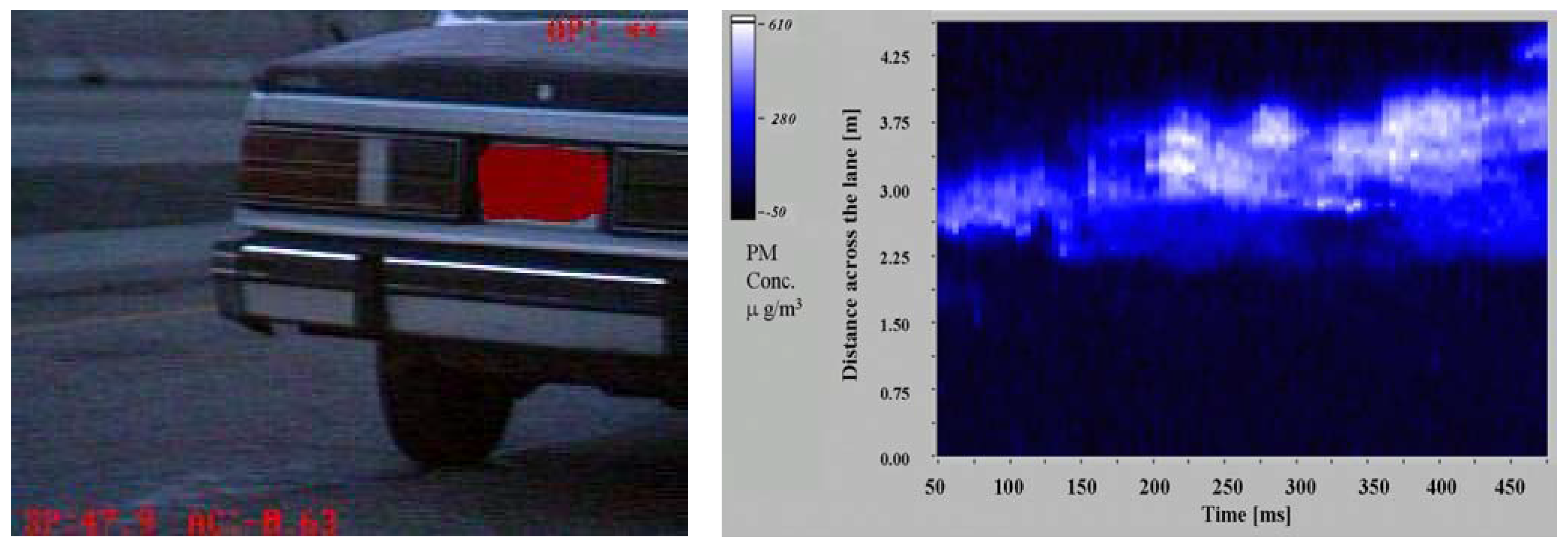
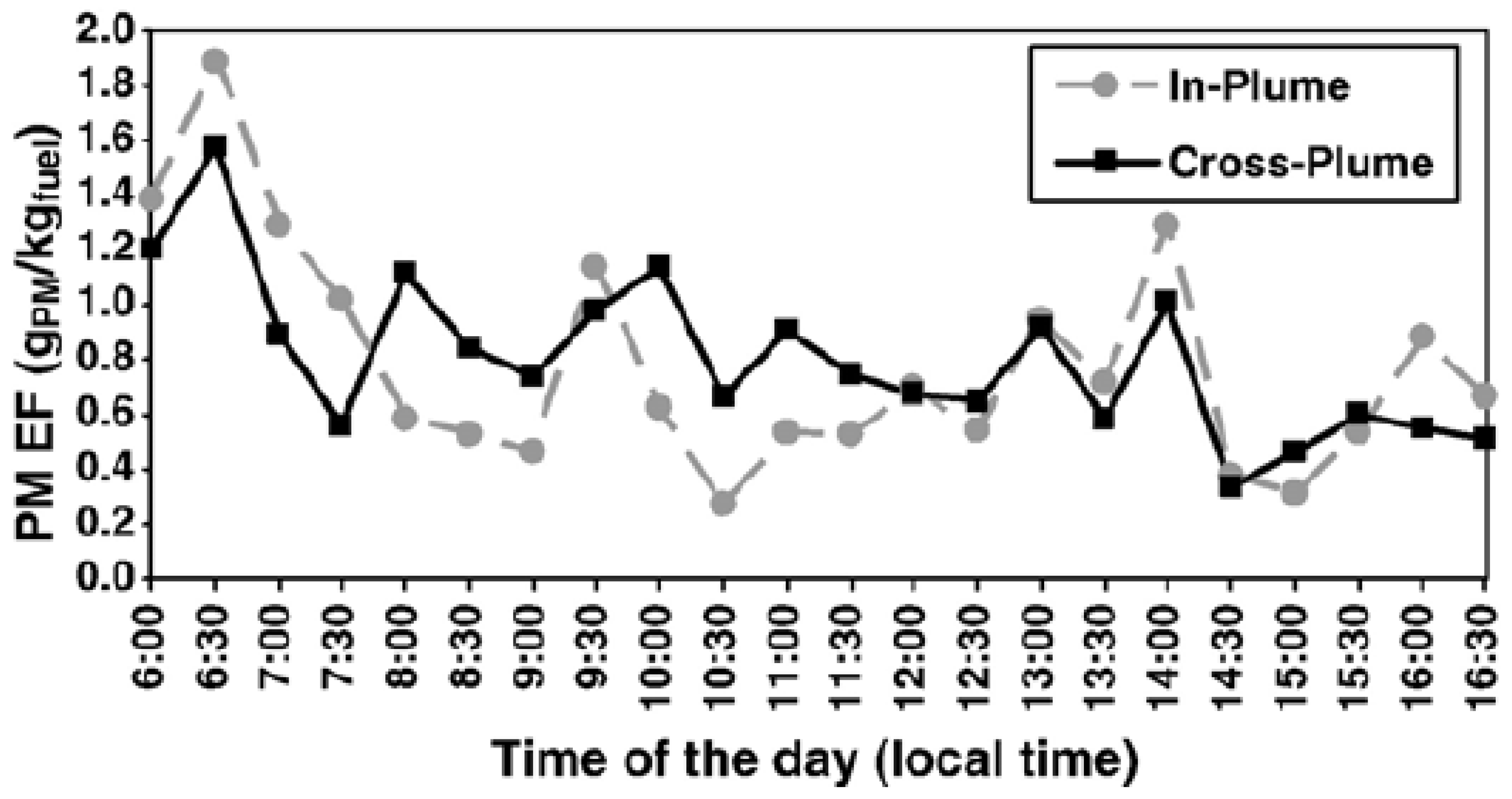
3.3. Calculation of Emission Factors from Backscattering and Extinction Measurements: An Example from the Field

The combined PM VERSS and gaseous VERSS system was used in the Southern Nevada Air Quality Study to measure emission factors for about 80,000 vehicles in the Las Vegas metropolitan area [14,17]. VERSS measurements from this study are analyzed in detail in Section 4.1. However, to further illustrate the concept of the PM VERSS, example data taken on May 8, 2002, in Las Vegas, NV, USA (at the northbound on-ramp from North Eastern Avenue onto I-515; 36.1684°N, 115.2487°W) from a medium-duty Isuzu W-series truck (model year 2000) powered by a 4.75-L diesel high-power engine are shown in Figure 6.

The excess PM mass column content as measured by the PM UV LiDAR and UV extinction channels (left y-axis) together with the consumed fuel mass column content (right y-axis) are shown in Figure 6a as a function of time. The consumed fuel mass column content was derived from the measurement of the excess CO₂ mass column content; see Equation (4) neglecting, for illustrative purposes, the CO and HC column contents that are generally low for diesel vehicles. After the vehicle passes the VERSS, measurements commence in the relatively concentrated exhaust plume resulting in high readings that then decay as the vehicle moves away from the beam path and the exhaust plume disperses into the ambient air. The PM LiDAR signal, the PM transmissometer signal, and the CO₂ signal decay about proportional to each other. PM emission factors, measured by LiDAR and transmissometer are obtained as the slopes of linear regressions between the respective excess PM mass column contents and the consumed fuel mass column content, obtained from the CO₂ measurement. Figure 6b shows these correlations with linear regressions (R² > 0.8) yielding fuel-based emission factors (EF_PM) of 2.5 ± 0.1 g/kg of fuel and 2.2 ± 0.1 g/kg of fuel (i.e., g of PM emitted/kg of fuel consumed) for the LiDAR and transmissometer measurement, respectively. These measurements yield a LiDAR ratio of 148 sr, very close (within ~10%) to that calculated for diesel PM (i.e., LR_diesel ~163 sr; Table 1) but 2.35 times larger than that calculated for spark ignition PM (i.e., LR_SI ~ 63 sr; Table 1), clearly identifying the vehicle as diesel powered.

Figure 6. Example data from a medium duty Isuzu W-series truck (model year 2000) powered by a 4.75-L diesel high-power engine. Data were taken on May 8, 2002, in Las Vegas, NV, USA (at the northbound on-ramp from N. Eastern Avenue onto I-515; 36.1684°N, 115.2487°W). (a) Excess PM mass column content from UV LiDAR and transmissometer and consumed fuel mass column content from CO₂ as a function of time. (b) Regression between PM and consumed fuel mass column contents yielding the PM emission factors from UV LiDAR and transmissometer as slopes in units of g of PM per kg of fuel [11].

Figure 6. Example data from a medium duty Isuzu W-series truck (model year 2000) powered by a 4.75-L diesel high-power engine. Data were taken on May 8, 2002, in Las Vegas, NV, USA (at the northbound on-ramp from N. Eastern Avenue onto I-515; 36.1684°N, 115.2487°W). (a) Excess PM mass column content from UV LiDAR and transmissometer and consumed fuel mass column content from CO₂ as a function of time. (b) Regression between PM and consumed fuel mass column contents yielding the PM emission factors from UV LiDAR and transmissometer as slopes in units of g of PM per kg of fuel [11].

The PM emission factors measured for this vehicle are comparable to the average of the diesel vehicles measured in Las Vegas by using the backscattering signals during 2001 (i.e., 2.1 ± 0.7 g/kg of fuel) and 2002 (i.e., 1.3 ± 0.3 g/kg of fuel) [14]. Most gasoline-powered vehicles have lower PM EFs, resulting in noisier measurements of the PM mass column content. However, even for gasoline-powered vehicles, the measurement of PM emissions from many vehicles allows entire vehicle groups and model year distributions of PM EFs to be determined. Note that in the case illustrated above, the standard errors for LiDAR and transmissometer measurement are comparable. Analysis of data from a large number of vehicles reveals that transmissometer measurements are less sensitive (by a factor of about 25) and have a positive bias due to turbulence (the laser beam moves relative to the photodiode). In addition, we should mention that these illustrative data were collected with a prototype system that had about a factor of 10 lower signal-to-noise ratio than the current system.

3.4. Field LiDAR Validation

During winter 2004, we conducted a field study near Boise, ID, USA on a fleet of school buses to evaluate the effects of biodiesel use on gaseous and PM fuel-based emission factors under real-world conditions [13]. During the same campaign we also measured the emissions of spark ignition vehicles passing by the sensor (described in Section 4.2). During the same campaign, and for a subset of the vehicle fleet, we collected data also by using an independent extractive in-plume sampling system. A detailed discussion of the in-plume system and its performances has recently been published [89,90]. The collocated deployment of the two systems provided a unique opportunity to evaluate the PM VERSS consistency with extractive analysis techniques.

The In-Plume system has an inlet (a tube set-up on the lane center and covered by a cable protector) secured in the center of the road to sample the vehicle emissions at road level. The sampled air is continuously drawn through the inlet to instruments that analyze it for both gasses and PM in real time. The PM mass is calculated from the volume size distribution measured in real time with a Dekati Electric Low Pressure Impactor (ELPI). An FTIR spectrometer is used for gaseous species measurement, and a LiCor analyzer is used for a secondary CO₂ measurement. The in-plume fuel-based EFs are calculated by rationing the PM and gaseous sample concentrations to the CO₂ concentrations after a background subtraction, in very similar fashion to the LiDAR PM EF calculations. When well distinguishable, individual peaks from the in-plume CO₂ concentration are identified and associated with specific vehicles, it is possible to calculate the individual vehicle PM EF and to compare it with the LiDAR-based PM EF. The averaged PM EFs measured by the two systems compared well for both diesel and gasoline vehicles (difference between averaged EFs measured by the two systems were less then 10% for diesel vehicles, and gasoline vehicles EFs agreed within 20%). However, due to the high traffic conditions, it was difficult to clearly identify individual vehicle emissions measured by both systems. To provide a statistically robust time comparison between the two systems, half-hour averaged PM EFs measured on March 4th, 2004 by the two systems were compared. Figure 7 shows that the measurements agree reasonably well between the in-plume and the VERSS, despite the uncertainties introduced by some vehicle mismatch between the two systems. A linear regression analysis of VERSS vs. in-plume half-hour average PM EFs yielded a slope of 0.7 ± 0.1, an intercept of 0.2 ± 0.2 and a correlation coefficient R² of 0.5 ± 0.2. The VERSS data compared reasonably well with the ELPI, which is a more established particle measurement method. However, ELPI tend to overestimate larger particles [91] (although correction algorithms are used to alleviate this problem [89]) and this might be a reason for why the linear regression slope between LiDAR and In-Plume is less than 1.

Figure 7. Time series for in-plume and VERSS systems for half-hour averaged PM EFs for the 4^th of March 2004. Overall average PM EFs are 0.78 ± 0.09 gPM/kgFuel and 0.80 ± 0.06 gPM/kgFuel for VERSS and in-plume system, respectively [13].

Figure 7. Time series for in-plume and VERSS systems for half-hour averaged PM EFs for the 4^th of March 2004. Overall average PM EFs are 0.78 ± 0.09 gPM/kgFuel and 0.80 ± 0.06 gPM/kgFuel for VERSS and in-plume system, respectively [13].

As an additional evaluation of the PM VERSS accuracy, we compared previous and independent on-road results with data collected with our PM VERSS in a large field campaign in the Las Vegas, NV, USA urban area (2001–2002) [14,17]. The results from this campaign are discussed in detail in Section 4.1. The PM EFs for heavy-duty diesel vehicles from different studies were distributed over a range of values (~0.6 to 2.5 g_PM/kg_Fuel) and our averaged PM VERSS EFs (1.3 to 2.1 g_PM/kg_Fuel) fell within this range. Average PM EFs from tunnel studies examining spark ignition vehicle emissions from large numbers of vehicles ranged from 0.03 to 0.072 g_PM/kg_Fuel, comparable to our averaged PM VERSS EFs (0.047 to 0.07 g_PM/kg_Fuel) [14].

4. Results from Various Field Deployments

In the following sub-sections we will review the results obtained from the field deployment of the LiDAR system in two different campaigns with different objectives; the goal is to demonstrate the system applicability and flexibility. The first campaign took place in Las Vegas, Nevada during 2000 and 2002 and is described in Section 4.1; the second campaign took place in Meridian, Idaho in 2004 and is discussed in Section 4.2. The performance of the UV LiDAR and transmissometer system was greatly improved after the first field campaign; the improved system has a 10-fold increase in the LiDAR signal-to-noise-ratio and includes more careful and accurate data processing. During the second campaign the minimum detection limit for the PM EF was therefore substantially lower (0.06 g_PM/kg_fuel vs. 0.25 g_PM/kg_fuel).

4.1. Las Vegas, Nevada 2000–2002: On-Ramp Freeway Vehicle Emissions

The commercial gaseous remote sensing device and the PM UV LiDAR and transmissometer VERSS were deployed at 10 different locations in the Las Vegas basin between 4 April 2000 and 16 May 2002 [14,17].

4.1.1. Campaign Objectives and Method

The main goal of the field campaign was to collect a large dataset of on-road vehicle emissions for gaseous as well as PM pollutants representative of the Las Vegas urban area. There were multiple specific objectives including: (a) determining the contribution of different vehicle type, age, weight, etc. to the total emission burden; (b) quantifying the dependence of vehicle emission with engine load; (c) determining how high emitters of one pollutant can contribute to other pollutants (e.g., is a high CO polluter also a high PM emitter?); (d) studying the effect of inspection and maintenance programs on gaseous pollution reduction; (e) quantifying the shape of the pollutant distributions across a statistically significant vehicle population; and (f) determining the feasibility of a PM remote sensing system and demonstrating its usefulness. Because the focus of this review is on the PM LiDAR and transmissometer system, we will discuss mostly the results directly relevant to PM EFs.

The sampling locations were selected to measure emissions from a broad range of vehicle types and ages distributed throughout the local area. The gaseous remote sensing provided measurements of the CO₂, CO, HC (in equivalent of propane) and NO column contents. As discussed above, CO₂, CO, and HC where used in conjunction with the LiDAR data to calculate PM EFs. A video camera recorded digital images of each vehicle’s license plate as it passed the test area. The data acquisition software stores these images for later license plate transcription. Images of 5,000–10,000 plates were typically collected during a day of sampling. Information about each vehicle’s emissions, speed, acceleration, and time of measurement were also recorded and linked to the other measurements. Nevada Department of Motor Vehicles (DMV) registration records for Clark County, NV from 1 January 2000 to 20 April 2002 contained 2.2 million records that included: license plate number, vehicle identification number, fuel type (i.e., spark or compression ignition), gross vehicle weight (GVW), and vehicle make and model year. The registration database did not designate whether a vehicle was a car, truck, or bus. These vehicle attributes were related to the field data via the plate ID. For 148,247 detected vehicles, 62% of the plume intensities were valid under strict criteria including a CO₂ signal above the background large enough to allow an accurate calculation of the emission factors. Of all the measurements, 42% had valid CO₂ values and valid Nevada license plates. Poor license plate image quality, dirty or obscured license plates, and many out of state vehicles were the predominant reasons for unmatched licenses.

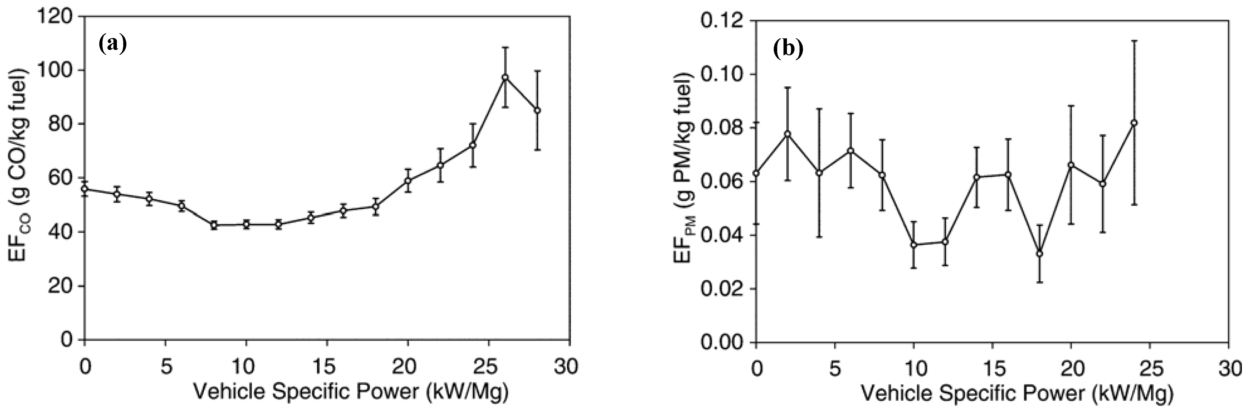
4.1.2. Emission Factors versus Vehicle Specific Power and Vehicle Age

An important parameter determining the emissions from vehicles is the engine load. Vehicle specific power (VSP) is defined as the power required by the engine to operate the vehicle at a given speed and acceleration divided by the mass of the vehicle [41]. The VSP in kW/Mg is estimated by the speed and acceleration data acquired with the VERSS as:

$$\begin{array}{l}VSP=\left(\frac{\text{Power}}{\text{Mass}}\right)=\left(\frac{P_{\text{Kinetic}}+P_{\text{Potential}}+P_{\text{Rolling}}+P_{\text{Internal Friction}}+P_{\text{Aerodynamic}}}{\text{Mass}}\right)\\ =v\cdot a(1+{\epsilon }_i)+g\cdot \text{grade}\cdot v+g\cdot C_R\cdot v+C_{if}\cdot v+\frac{1}{2}{\rho }_a{C}_D\frac{A}{\text{Mass}}{(v+v_W)}^2\cdot v\\ \approx 1.1\cdot v\cdot a+9.81\cdot \text{grade}\cdot v+0.213\cdot v+0.000305\cdot {(v+v_W)}^2\cdot v\end{array}$$

(20)

where P_Kinetic, P_Potential, P_Rolling, P_{Internal Friction}, and P_Aerodynamic represent the power needed to accelerate the vehicle at a specified velocity, the power needed to overcome the gravitational force (i.e., on a sloped road), the power needed to overcome the vehicle internal friction and the aerodynamic drag, respectively. The variables v and v_W are the vehicle speed and headwind speed in m/s, respectively. The variable a is the acceleration in m/s² and grade is the rise/run (i.e., arctan(slope in deg)). ε_i is the unitless ‘mass factor’ that accounts for the translational mass of the rotating components (i.e., wheels, axles, crankshaft, etc.). The coefficient of rolling resistance C_R and the coefficient of aerodynamic drag C_D are unitless. C_if is the internal friction factor with units of m/s² and ρ_a is the density of air (kg/m³). The frontal area A has units of m² and vehicle mass (in kg) are based on typical values for cars or light trucks. Jimenez [41] estimates values for all terms except v, a, and grade so that VSP can be calculated for each vehicle from variables measured during routine exhaust remote sensing operations.

VSP is also important to compare vehicle remote sensing measurements with standardized vehicle driving cycles (such as the federal test procedure (FTP)) that are used to estimate emission factors using numerical models such as the MOBILE model developed and used by the US Environmental Protection Agency [92]. For light-duty gasoline powered vehicles measured with the VERSS during the Las Vegas study, the average VSP was 9.5 kW/Mg. Acceleration from 0 to 60 miles/h in 15 s with a VSP of 33 kW/Mg is an example of hard acceleration that is a common mode on unobstructed freeway onramps. The average VSP measured was lower than the normal onramp mode because motorists tend to reduce speed and exercise caution in the vicinity of the VERSS traffic control signs and cones.

Figure 8 shows an example of the relationships between VSP and remotely sensed emissions of CO and PM for light duty gasoline vehicles. For each vehicle, the VSP was calculated using Equation 20 and binned into the aggregate averages. The uncertainty was calculated from the statistic of each averaged group. CO emissions (panel (a) in Figure 8) initially decrease by approximately one-third from 60 to 40 g/kg fuel over the VSP range of 0–8 kW/Mg. Emissions are generally stable between 8 and 18 kW/Mg. Above 18 kW/Mg, emissions rose from 50 g/kg fuel to approximately 100 g/kg fuel at a VSP of 26 kW/Mg. This increase at high loads has been measured in many other studies in the US and has been attributed to command enrichment in the vehicle to boost power output. These relationships of VSP vs. CO are consistent with other laboratory and on-road studies. A similar graph (although noisier than for CO) can be seen in the remotely measured PM EFs (panel (b) in Figure 8).

Figure 8. Panel (a) CO emission factors vs. the Vehicle Specific Power, panel (b) PM emission factors vs. the Vehicle Specific Power [17].

Figure 8. Panel (a) CO emission factors vs. the Vehicle Specific Power, panel (b) PM emission factors vs. the Vehicle Specific Power [17].

Figure 9. PM emission factors vs. the vehicle age and PART5 numerical simulation [17].

Figure 9. PM emission factors vs. the vehicle age and PART5 numerical simulation [17].

As another example of quantitative information provided by the PM VERSS, Figure 9 shows the increase of emissions with the vehicle age due to poor maintenance, older (or non existing) emission technology, etc. On the same figure the result of the PART5 numerical simulation are also reported. PART5 was the PM module of the MOBILE6 EPA model that was used to predict PM emissions during the study; PART5 results were compared to the measured emissions. Details about the input parameters of the models are described by Kuhns et al. [93]. It is evident from the figure that although on average the emission calculated from the model and measured on the road are close to each other, the assumption of constant emission with vehicle age does not apply to the Las Vegas traffic; older vehicles are higher PM emitters, consistent with CO, HC, and NO EFs from the same study [17].

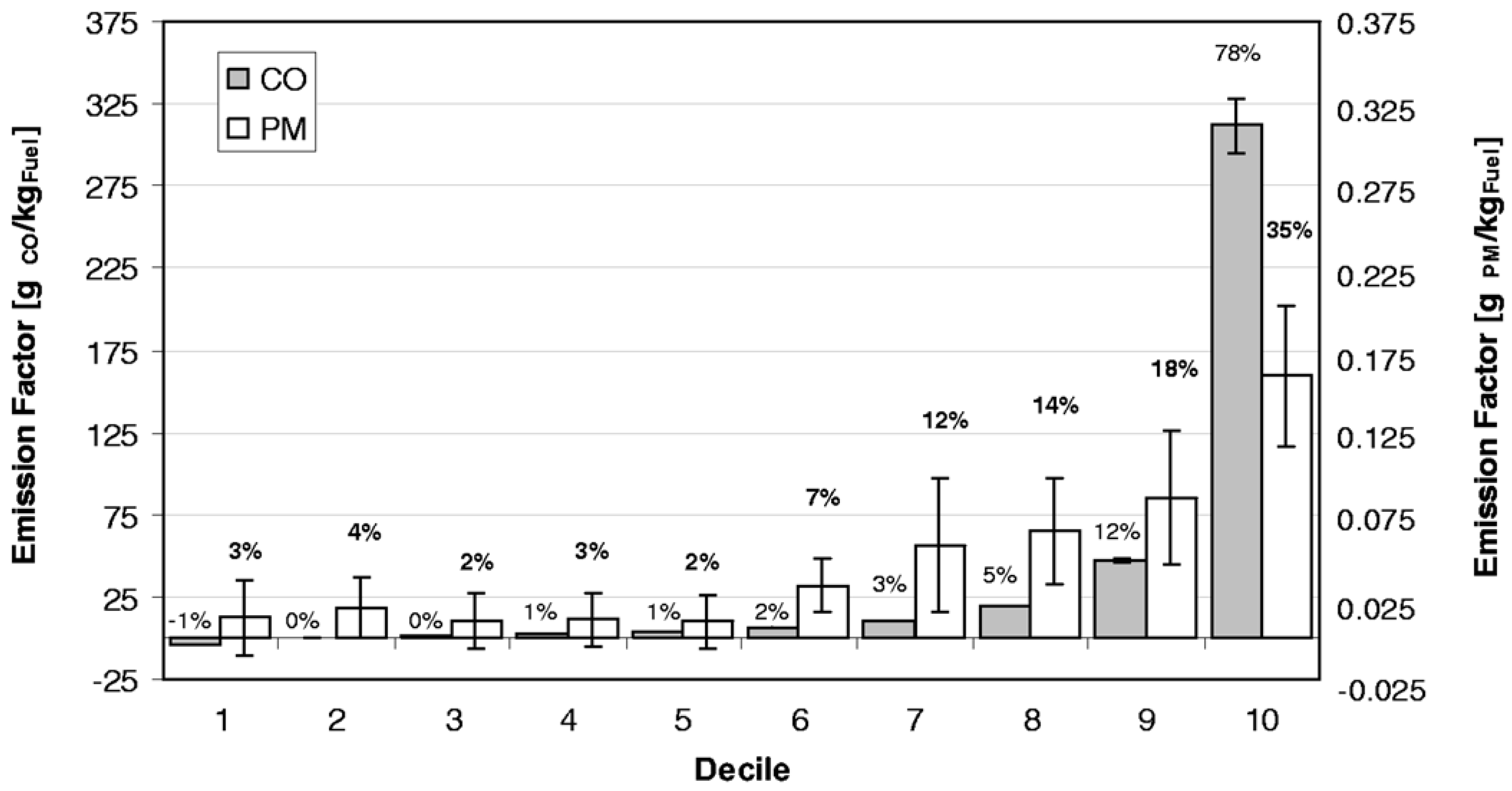
4.1.3. Particulate Matter Emission Statistics and Distribution Skewness

For this study the mean PM emission factors for the 2001 and 2002 field campaigns for spark ignition vehicles were 0.07 ± 0.013 and 0.047 ± 0.009 g/kg-fuel, with medians of 0.008 ± 0.004 and 0.013 ± 0.004 g/kg-fuel, respectively. The wide differences between median and mean is due to the skewness of the emission distribution. The fact that emission distributions are highly skewed implies that only a few highly polluting vehicles contribute to the majority of the overall fleet emission. The contribution (expressed in %) of the highest-emitting 10% vehicles of a fleet is often used as a measure of the skewness of the emission distribution. A severe skewness has been measured for the CO emission factors with often just 10% of the vehicles (indicated as gross polluters) contributing to more than 70% of the overall fleet emission in different campaigns and different urban areas around the world. Due to the lack of PM remote sensing studies before those summarized here, PM skewness was estimated by road side studies [19] or by theoretical extrapolations; however no direct measurement was possible on large fleets.

The quantitative calculation of the skewness of emission factor distributions however is complicated by the presence of instrumental noise in the measurements. To estimate the skewness and simultaneously estimate the system minimum detection limit we used a fitting approach. The measured data are considered as a combination of a real positive emission signal plus a noise component (which may not be normally distributed). The assumption is that these two components are independent and they randomly add up to the measured value [14,41,94]. For this study, the distribution of slopes was fit to a combination of distributions, one symmetric around zero to represent the noise, and another one limited to positive values and with some amount of skewness to represent the emissions. Different distributions were tested; for PM emissions, the best fit was obtained with a double-sided exponential distribution representing the noise, combined with a Weibull distribution representing the emissions. The method was used to estimate the detection limit of the system as one sigma of the noise distribution. The first generation of the PM LiDAR used in this campaign had a detection limit for an individual vehicle of 0.25 g_PM/kg_fuel (to be compared to a detection limit of 5.7 g_PM/kg_fuel for the transmissometer alone), while the second generation system (used in the field campaign described in Section 3.2) had a detection limit of 0.06 g_PM/kg_fuel. Although the LiDAR signal to noise ratio was improved by a factor of 10 between the two systems, the detection limit improved only by a factor of ~4, this is because the emission factors depends also on other aspects, including the CO₂ column content measurement noise and the fact that the CO₂ IR beam and the UV LiDAR laser beam were not exactly collocated in space. The sensitivity of the fit to the distribution parameters yields a lower limit for the skewness of the emission distribution, indicating that for spark ignition vehicles, the highest 10% of the PM measurements contribute more than 80% of the fleet PM EFs.

Due to the skewness of the emission factors, statistical spreads cannot be calculated by simply employing parametric statistical methods based on normal distributions. Therefore the 95% confidence interval also reported above for means and medians were calculated by using a bootstrap technique, resampling with replacement from the raw data. The spread of each mean and median was determined by constructing a frequency distribution of 50,000 bootstrap estimates.

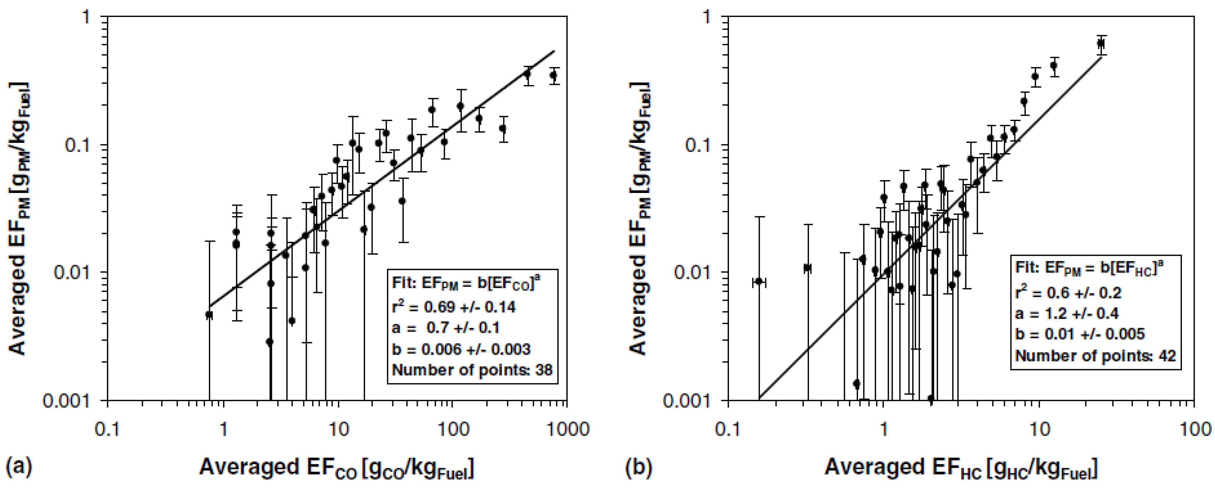
4.1.4. Correlation of Particulate Emission with Gaseous Emissions

Positive correlations between PM and CO or HC emission factors would be expected because excessive emissions are caused by non-ideal combustion conditions and/or poor oxidation efficiency of the catalytic converter. If emissions for several pollutants on individual vehicles would be consistently and quantitatively related to one another, there would be no need to measure each pollutant individually. Correlation coefficients for PM emission factors vs. CO and HC for individual vehicles however were low even when only measurements in a limited range of road load or only higher emitters were included in the analysis. The correlations had a maximum of 0.02 for PM vs. HC, and 0.01 for PM vs. CO EFs. Multivariate correlations (e.g., PM EFs as a function of both CO and HC EFs) were also considered, but showed negligible improvement. These weak correlations are definitely insufficient to estimate PM EFs from the CO and HC concentrations as measured by traditional remote sensing systems or commonly measured in inspection and maintenance tests [15].

Previous studies have shown good correlations between PM and CO distance-based EFs (i.e., mass of pollutant emitted per distance traveled) from dynamometer tests for individual diesel vehicles. However, the regression slope depends on the vehicle tested. This does not extend to the large number of different vehicles measured by the PM remote sensing system used in this study.

Relationships among pollutants were more evident for averaged data. Figure 10 compares the averaged PM vs. the averaged CO and HC measurements. The data were sorted by increasing independent CO EFs and then divided into 50 groups. CO and PM average EFs and standard errors were calculated for each group. Only positive averages were plotted and used in the regression calculation. The results of power fit y = b·x^a are reported in the text box. The uncertainties of the regression parameters represent the 95% level confidence limit calculated by bootstrap with resampling technique. After this substantial averaging, positive correlations were evident [15].

Figure 10. Average PM emission factors vs. CO (a) and vs. HC (b) emission factors [15].

Figure 10. Average PM emission factors vs. CO (a) and vs. HC (b) emission factors [15].

It is important to determine if CO gross polluting vehicles are also PM gross polluting vehicles and vice versa. If these two categories overlap, then a CO remote sensing system could identify high PM emitters. This is a very important issue for regulatory, enforcement and inspection purposes. In Figure 11 we report a decile graph where the emission data have been sorted by increasing CO emission factors that were collected during the Las Vegas experiment. The figure shows that more than 78% of the CO fleet emission is due to only 10% of the vehicles. However, the same 10% vehicles contribute only 35% of the total PM emissions, whereas the dirtiest 10% PM emitters contribute more than 80% of the PM emissions. Based on this analysis, not all the highest CO emitters are also high PM emitters; therefore a PM sensing system is indeed necessary not only to quantify the PM emissions, but also to individuate high PM emitters [14]. The fact that the lower bin has a small negative average is due to the substantial noise present in the measured emission factors. The measurements are performed in just 0.5 seconds and on a busy road with substantial vibrations and environmental interferences, therefore a considerable amount of noise is expected. A detailed discussion and analysis of the noise in vehicle remote sensing measurements is presented by Mazzoleni et al. [95].

Figure 11. Contributions of lowest to highest CO emitters to the CO and PM emission factors for spark-ignition vehicles measured in Las Vegas in 2002. The error bars represent the 95% confidence interval for the respective decile mean. The percent above each column indicates the contribution to the fleet emission factor of CO or PM [14].

Figure 11. Contributions of lowest to highest CO emitters to the CO and PM emission factors for spark-ignition vehicles measured in Las Vegas in 2002. The error bars represent the 95% confidence interval for the respective decile mean. The percent above each column indicates the contribution to the fleet emission factor of CO or PM [14].

To investigate the possibility that other pollutants might overlap better with PM and further quantify the degree of overlap between different pollutants categories, we report in Table 4 the overlap between the groups of emitters belonging to the highest 10% emitters for the different pollutants.

Table 4. Degree of overlap between the 10% highest emitters within the different pollutant categories.

	Number of Vehicles	Fraction of Measured Fleet
Total number of vehicles	13,786
No high emitters in any category	9,975	72.36%
High emitters in one category		Total: 18.20%
CO	556	4.03%
HC	326	2.36%
NO	812	5.89%
PM	816	5.92%
High emitters in two categories		Total: 6.84%
CO & HC	436	3.16%
CO & NO	49	0.36%
CO & PM	56	0.41%
HC & NO	194	1.41%
HC & PM	70	0.51%
NO & PM	137	0.99%
High emitters in three categories		Total: 2.35%
CO & HC & NO	62	0.45%
CO & HC & PM	174	1.26%
CO & NO & PM	9	0.07%
HC & NO & PM	79	0.57%
High emitters in all four categories	38	0.28%

Table 4. Degree of overlap between the 10% highest emitters within the different pollutant categories.

	Number of Vehicles	Fraction of Measured Fleet
Total number of vehicles	13,786
No high emitters in any category	9,975	72.36%
High emitters in one category		Total: 18.20%
CO	556	4.03%
HC	326	2.36%
NO	812	5.89%
PM	816	5.92%
High emitters in two categories		Total: 6.84%
CO & HC	436	3.16%
CO & NO	49	0.36%
CO & PM	56	0.41%
HC & NO	194	1.41%
HC & PM	70	0.51%
NO & PM	137	0.99%
High emitters in three categories		Total: 2.35%
CO & HC & NO	62	0.45%
CO & HC & PM	174	1.26%
CO & NO & PM	9	0.07%
HC & NO & PM	79	0.57%
High emitters in all four categories	38	0.28%

It is evident that, if the goal is to individuate gross polluters in each individual pollutant category, a technique specific to each pollutant needs to be deployed on the road [15].

4.2. Meridian, Idaho 2004: School-Busses Emissions, Petroleum- versus Bio-Diesel

In this section, we present results from another application of the PM remote sensing system. In winter 2004, we conducted an experiment designed to measure real-world changes in on-road gaseous and PM emissions for an in-use fleet of school buses before and after a switch from winter petroleum diesel fuel blend to a blend of 20% (by volume) biodiesel and 80% petroleum diesel (B20) [13]. Real-world conditions of this study were documented including odometer readings of the school buses, bus models, bus engine loads, maintenance records, environmental conditions (i.e., the winter atmospheric conditions), fuel type, and fuel quality.

4.2.1. Measurements Description and Field Campaign Objectives

Biodiesel is an alternative, partially renewable source of energy prepared by the trans-esterification of vegetable oils or waste animal fats [96] and is composed of carbon extracted by the photosynthetic process. The use of biodiesel reduces the net anthropogenic CO₂ emissions into the atmosphere. Diesel engines however, emit substantial amounts of pollutants such as nitrogen oxides and PM. Of particular concern is the exposure of children to these pollutants in school buses during their daily commute [97]. Previous studies showed that the use of biodiesel resulted in a reduction of carbon monoxide, hydrocarbons, and PM emissions, with a slight increase in nitrogen oxides emissions with respect to vehicles fueled by petroleum diesel. For example, a USA EPA comprehensive document summarizing the results of many previous studies reports reductions of 10.1% in PM, 21.1% in HC and 11.0% in CO with an increase of 2.0% in nitrogen oxides for blends of 20% biodiesel and 80% petroleum diesel [98]. These studies however were performed under controlled laboratory conditions, or on individual vehicles using on-board emission measurement equipment; prior to emission testing, fuels were subjected to quality analyses and when analyses indicated that the fuels were not in compliance with the appropriate specification (USA ASTM D975 for petroleum diesel and USA ASTM D6751 for biodiesel), the emission tests were not performed. Our study was designed to verify if these positive results would hold in realistic environmental conditions (meteorological conditions, vehicle type, maintenance and age, driving conditions, etc.) on the road and using commercially available (not prescreened) fuel to simulate a typical biodiesel usage situation.

The buses used in this study were originally operating on a winter fuel blend of 70% 2-D and 30% 1-D diesel fuels (phase I) and were then switched to a blend of 80% 2-D, 20% biodiesel and 0.1% anti-gelling additive (phase II). The blending 2-D fuel in both phases was obtained from the same local provider. Fuel testing after the experiment indicated that the 2-D fuels were within the ASTM D975 specifications. The fuel change to B20 occurred with no engine modifications or fuel system alterations. Five of the school buses had switched to B20 18 months prior to the fuel switch for the rest of the fleet as control vehicles.

The emission testing system was located on a dead end road at a school-bus depot in Meridian, ID, USA and only one vehicle at a time passed by the sampling system. The school bus depot employees and the students and faculty of a local high school passed through the site as well, with mostly spark ignition passenger vehicles that were hot stabilized from the commute. The vehicles were parked and left in parking lots for most of the day. The distance between each individual vehicle parking spot and the sampling location were less than 250 m. Both buses and private vehicles leaving the bus depot had typically been parked for several hours and their engines were operating under cold-start conditions (i.e., less than 2 minutes of engine operation after a 5+ hour cold soak). The vehicle driving direction was therefore associated with cold-start (leaving the site) and hot-stabilized (arriving to the site) engine conditions. Therefore, the site-set-up allowed also studying the effects of engine temperature on pollutants emissions.

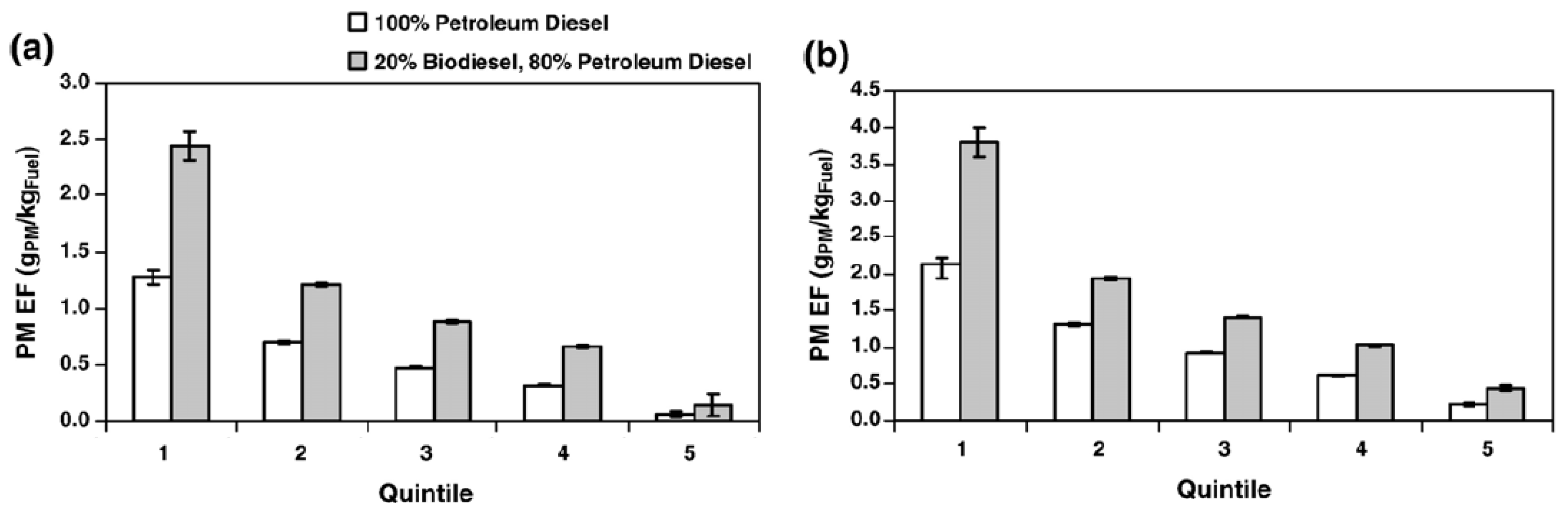
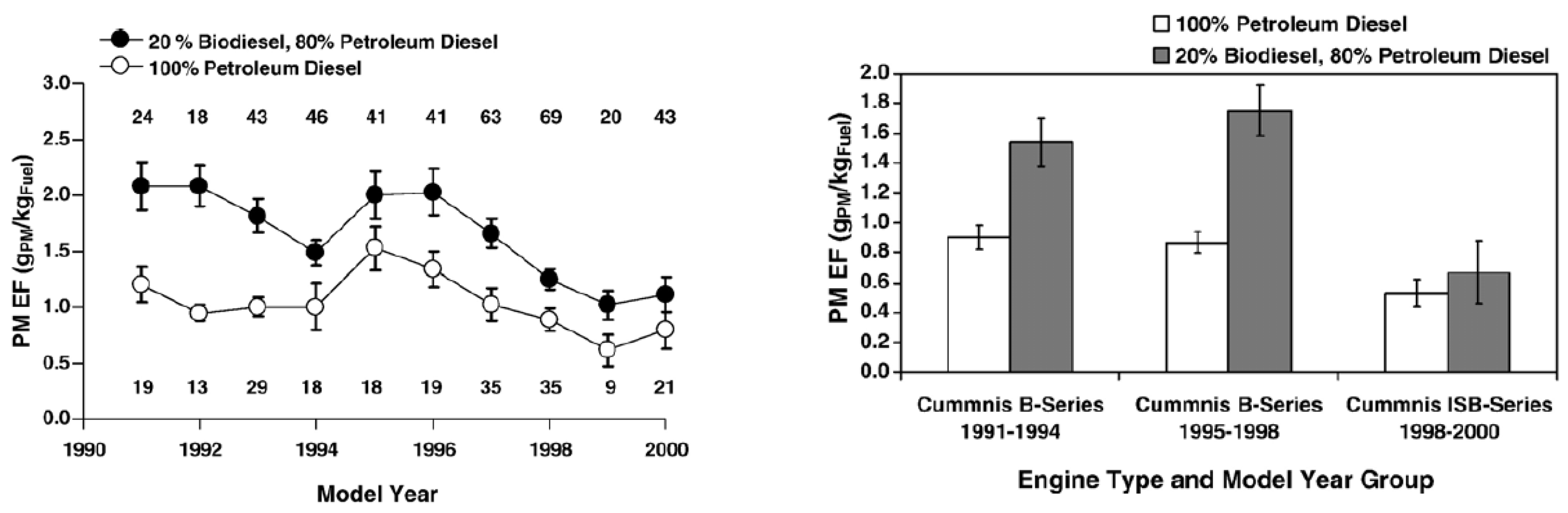
4.2.2. Buses and Passenger Vehicles Particulate Matter Emissions

For the buses, the largest changes in EFs were observed for PM. Cold-start PM EFs were 65% ± 8% higher and hot-stabilized PM EFs were 88% ± 11% higher after the buses had been switched to B20, contrary to what was expected from previous laboratory studies. Median EFs showed a similar pattern (Table 5). A comparison of quintile distributions for PM EFs showed that the difference between B20 and petroleum diesel PM EFs was consistent over the entire fleet and not limited to only the highest emitting vehicles (Figure 12). Finally, we analyzed the increased PM emission factors in the school buses as a function of model year and engine type to see if the increase depended on any of these variables. In Figure 13 we report the results of such stratification. PM EFs for buses running on B20 were significantly higher than EFs for buses running on petroleum diesel for every model year tested.

Engine type is generally a stronger factor that influences PM EFs than is vehicle model year. Panel (b) of Figure 13 indicates that the average PM EFs are related to engine type. There are no evident physical differences between the Cummins B-Series engines from model years 1991–1994 and model years 1995–1998. Emissions were generally higher from the latter model year engines, so the results were stratified along what appeared to be a natural break in the data. In the figure we show that the newer Cummins ISB-Series engines had lower PM EFs and were less prone to increased PM emissions when using B20. At the end of the study (as a blind test) we analyzed the fuel and found that the B20 was not compliant with the ASTM standards and contained excess of glycerin which might cause flow restrictions in the fuel lines. The ISB engine has a computer controlled fuel injection system and may have been able to compensate for restricted fuel flows associated with off-specification B20 Fuels.

Table 5. Particulate matter emission factors (±68% confidence limits) for the school busses powered by petroleum diesel and a B20 biodiesel blend (20% biodiesel and 80% petroleum diesel) and for passenger vehicles (mostly gasoline cars) for both cold engine and hot engine conditions. The control buses were powered with B20 since few months before the beginning of the experiment.

	Average	Median	Number
School Buses with Petroleum Diesel - hot engine	0.57 ± 0.03	0.47 ± 0.03	241
School Buses with Petroleum Diesel - cold engine	1.05 ± 0.05	0.92 ± 0.05	234
School Buses with B20 - hot engine	1.07 ± 0.06	0.89 ± 0.03	291
School Buses with B20 - cold engine	1.73 ± 0.07	1.41 ± 0.04	494
Control Buses Phase I – cold engine†	1.62 ± 0.45	-	5
Control Buses Phase II – cold engine†	1.76 ± 0.38	-	11
Passenger Vehicles Phase I - hot engine	0.22 ± 0.03	0.16 ± 0.02	124
Passenger Vehicles Phase I - cold engine	0.34 ± 0.04	0.16 ± 0.02	264
Passenger Vehicles Phase II - hot engine	0.18 ± 0.04	0.06 ± 0.01	354
Passenger Vehicles Phase II - cold engine	0.43 ± 0.04	0.19 ± 0.02	483

^†Control buses could be identified only by using their license plate. The license plate was readable only for vehicles leaving the bus-depot, due to the orientation of the digital camera, therefore only cold-engine conditions could be analyzed for this vehicle group.

Table 5. Particulate matter emission factors (±68% confidence limits) for the school busses powered by petroleum diesel and a B20 biodiesel blend (20% biodiesel and 80% petroleum diesel) and for passenger vehicles (mostly gasoline cars) for both cold engine and hot engine conditions. The control buses were powered with B20 since few months before the beginning of the experiment.

	Average	Median	Number
School Buses with Petroleum Diesel - hot engine	0.57 ± 0.03	0.47 ± 0.03	241
School Buses with Petroleum Diesel - cold engine	1.05 ± 0.05	0.92 ± 0.05	234
School Buses with B20 - hot engine	1.07 ± 0.06	0.89 ± 0.03	291
School Buses with B20 - cold engine	1.73 ± 0.07	1.41 ± 0.04	494
Control Buses Phase I – cold engine†	1.62 ± 0.45	-	5
Control Buses Phase II – cold engine†	1.76 ± 0.38	-	11
Passenger Vehicles Phase I - hot engine	0.22 ± 0.03	0.16 ± 0.02	124
Passenger Vehicles Phase I - cold engine	0.34 ± 0.04	0.16 ± 0.02	264
Passenger Vehicles Phase II - hot engine	0.18 ± 0.04	0.06 ± 0.01	354
Passenger Vehicles Phase II - cold engine	0.43 ± 0.04	0.19 ± 0.02	483

^†Control buses could be identified only by using their license plate. The license plate was readable only for vehicles leaving the bus-depot, due to the orientation of the digital camera, therefore only cold-engine conditions could be analyzed for this vehicle group.

Figure 12. Quintile distributions of particulate matter (PM) emission factors (EFs) for school buses with hot-stabilized and cold-start engine conditions. Panel (a) represents results obtained in hot engine conditions; panel (b) represents cold-start conditions only [13].

Figure 12. Quintile distributions of particulate matter (PM) emission factors (EFs) for school buses with hot-stabilized and cold-start engine conditions. Panel (a) represents results obtained in hot engine conditions; panel (b) represents cold-start conditions only [13].

Figure 13. Particulate matter (PM) emission factors (EFs) for school buses with cold-start engine conditions stratified by model year (panel (a)) and engine type (panel (b)) [13].

Figure 13. Particulate matter (PM) emission factors (EFs) for school buses with cold-start engine conditions stratified by model year (panel (a)) and engine type (panel (b)) [13].

From Table 5 we can therefore gather a series of additional interesting conclusions: (a) the skewness of diesel PM emissions is low (as demonstrated by the similarity of means and medians), meaning that most vehicle emits substantially high concentrations of PM per mass of fuel burned, similarly to what has been found in previous studies for diesel gaseous emissions [48]; (b) passenger vehicles (mostly gasoline-powered) emitted substantially less PM, (c) a higher degree of skewness is measured for passenger vehicles than for buses, meaning that a small number of high polluting passenger vehicles contribute the most to the total fleet PM emission in agreement with what found in Las Vegas (see Section 4.1) ; (d) cold-engine PM emissions are much higher than hot-stabilized engine emissions (up to a factor of ~2) for buses as well as for passenger vehicles; (e) B20-powered buses emitted much more PM than petroleum diesel powered buses, presumably because of the poor biodiesel fuel quality sold in the area; (f) control buses that were powered with B20 over the entire study period emitted consistently higher PM per mass of fuel than the petroleum-diesel-powered vehicles, corroborating the results found in point (e) and demonstrating that the PM LiDAR-based remote sensing system data were not biased between the two phases of the study by confounding factors (such as meteorological conditions) or instrumental drifts. These types of analysis and detailed data stratification were possible only because the remote sensing system is capable of collecting large amount of individual-vehicle data allowing for the calculation of statistical significant means and medians despite the intrinsic vehicle-to-vehicle and time variability.

5. Conclusions

In the first section of this paper we introduced the challenges associated with vehicle emission research and discussed the significance of remote sensing applications. In the second section we discussed the theoretical foundations for the calculation of fuel based emission factors. In the third section of this paper, we reviewed the development of a UV LiDAR and transmissometer system applied to roadside measurements of PM emissions from vehicles. We presented the detailed instrumental characteristics, limitations, and sensitivity. We discussed the calibration procedure and the field deployment setup. We then described the theoretical arguments used to derive PM mass concentrations from the backscattering LiDAR and transmissometer measurements, and used to justify the choice of the instrument specifications (most importantly, the laser wavelength). In the forth section we reviewed some of the most interesting results gathered with the system in different field deployments.

The usefulness of a UV LiDAR as a remote sensing system to measure PM vehicle emissions is evident from the ability of the system to collect a large amount of data for individual vehicles and the consequent possibility to stratify the data across many significant parameters. The ability to collect data for a large number of vehicles, and at the same time maintaining the individual vehicle specificity, is the most unique aspect of VERSS that makes it extremely useful to untangle the complexity of real-world vehicle emissions.

A LiDAR approach to PM emission is also much more sensitive than other traditionally used methods, such as opacity meters. Using the system described here, it was possible to measure the effects that vehicle engine load, vehicle model year, vehicle type and fuel, engine conditions (cold vs. hot), etc. have on the PM emissions from both diesel and gasoline-powered vehicles, and to clearly quantify these dependences. Correlations of PM with CO and HC emissions were also explored. It was also shown that although some new fuel (as for example biodiesel) might hold promise to reduce emissions, these reductions can be negated or even reversed if the fuel quality is not controlled at the point of distribution. These broad applications demonstrate the flexibility and power of the VERSS technique.

Remote sensing in general, and UV LiDAR and transmissometry in the specific case of PM emissions, represent technological advancements that should be exploited to study vehicle emissions in real-world conditions, and to measure the effectiveness of new technologies, fuels or emission control strategies. Some of the limitations intrinsic to remote sensing measurement approaches can be compensated by using this technology in combination with other techniques such as onboard measurements and roadside dynamometer studies. A hybrid approach of this sort, incorporating the strengths and uniqueness of remote sensing technologies, represents the future of vehicle emission research.

References and Notes

1. Pope, C.A.; Dockery, D.W. Health effects of fine particulate air pollution: Lines that connect. J. Air Waste Manage. Assoc. 2006, 56, 709–742. [Google Scholar] [CrossRef]
2. Solomon, S.; Qin, D.; Manning, M.; Chen, Z.; Marquis, M.; Averyt, K.B.; Tignor, M.; Miller, H.L. Climate Change 2007: The Physical Science Basis; IPCC Secretariat: Geneva, Switzerland, 2007. [Google Scholar]
3. Watson, J.G. 2002 critical review—Visibility: science and regulation. J. Air Waste Manage. Assoc. 2002, 52, 628–713. [Google Scholar] [CrossRef]
4. Matsui, T.; Beltrán-Przekurat, A.; Niyogi, D.; Pielke, R.A., Sr.; Coughenour, M. Aerosol light scattering effect on terrestrial plant productivity and energy fluxes over the eastern United States. J. Geophys. Res. 2008, 113. [Google Scholar] [CrossRef]
5. Bonazza, A.; Brimblecom, P.; Grossi, C.M.; Sabbioni, C. Carbon in black crusts from the tower of London. Environ. Sci. Technol. 2007, 41, 4199–4204. [Google Scholar] [CrossRef] [PubMed]
6. Hansen, J.; Sato, M.; Ruedy, R.; Lacis, A.; Oinas, V. Global warming in the twenty-first century: An alternative scenario. Proc. Nat. Acad. Sci. USA 2000, 97, 9875–9880. [Google Scholar] [CrossRef] [PubMed]
7. Chazette, P.; Liousse, C. A case study of optical and chemical ground apportionment for urban aerosols in Thessaloniki. Atmos. Environ. 2001, 35, 2497–2506. [Google Scholar] [CrossRef]
8. Moosmüller, H.; Chakrabarty, R.K.; Arnott, W.P. Aerosol light absorption and its measurement: A review. J. Quant. Spectrosc. Radiat. 2009, 110, 844–878. [Google Scholar] [CrossRef]
9. Moosmüller, H.; Arnott, W.P. Particle optics in the Rayleigh Regime. J. Air Waste Manage. Assoc. 2009, 59, 1028–1031. [Google Scholar] [CrossRef]
10. Bond, T.; Bergstrom, R. Light absorption by carbonaceous particles: An investigative review. Aerosol Sci. Tech. 2006, 40, 27–67. [Google Scholar] [CrossRef]
11. Moosmüller, H.; Mazzoleni, C.; Barber, P.W.; Kuhns, H.D.; Keislar, R.E.; Watson, J.G. On-road measurement of automotive particle emissions by ultraviolet lidar and transmissometer: Instrument. Environ. Sci. Technol. 2003, 37, 4971–4978. [Google Scholar] [CrossRef] [PubMed]
12. Barber, P.W.; Moosmüller, H.; Keislar, R.E.; Kuhns, H.D.; Mazzoleni, C.; Watson, J.G. On-road measurement of automotive particle emissions by ultraviolet Lidar and transmissometer: Theory. Meas. Sci. Technol. 2004, 15, 2295–2302. [Google Scholar] [CrossRef]
13. Mazzoleni, C.; Kuhns, H.D.; Moosmüller, H.; Witt, J.; Nussbaum, N.J.; Chang, M.C.O.; Parthasarathy, G.; Nathagoundenpalayam, S.K.K.; Nikolich, G.; Watson, J.G. A case study of real-world tailpipe emissions for school buses using a 20% biodiesel blend. Sci. Total Envir. 2007, 385, 146–159. [Google Scholar] [CrossRef] [PubMed]
14. Mazzoleni, C.; Kuhns, H.D.; Moosmüller, H.; Keislar, R.E.; Barber, P.W.; Robinson, N.F.; Watson, J.G. On-road vehicle particulate matter and gaseous emission distributions in Las Vegas, Nevada, compared with other areas. J. Air Waste Manage. Assoc. 2004, 54, 711–726. [Google Scholar] [CrossRef]
15. Mazzoleni, C.; Moosmüller, H.; Kuhns, H.D.; Keislar, R.E.; Barber, P.W.; Nikolic, D.; Nussbaum, N.J.; Watson, J.G. Correlation between automotive CO, HC, NO, and PM emission factors from on-road remote sensing: implications for inspection and maintenance programs. Transp. Res. PT D-Transp. Enviro. 2004, 9, 477–496. [Google Scholar] [CrossRef]
16. Mazzoleni, C.; Kuhns, H.D.; Moosmüller, H. Pollution reduction using biofuels: from the laboratory to the real world. In New Research on Biofuels; Wright, J.H., Evans, D.A., Eds.; Nova: New York, NY, USA, 2008; pp. 117–121. [Google Scholar]
17. Kuhns, H.D.; Mazzoleni, C.; Moosmüller, H.; Nikolic, D.; Keislar, R.E.; Barber, P.W.; Li, Z.; Etyemezian, V.; Watson, J.G. Remote sensing of PM, NO, CO, and HC emission factors for on-road gasoline and diesel engine vehicles in Las Vegas, NV. Sci. Total Envir. 2004, 322, 123–137. [Google Scholar] [CrossRef] [PubMed]
18. Li, W.; Collins, J.F.; Durbin, T.D.; Huai, T.; Ayala, A.; Full, G.; Mazzoleni, C.; Nussbaum, N.J.; Obrist, D.; Zhu, D.; Kuhns, H.D.; Moosmüller, H. Detection of gasoline vehicles with gross PM emissions. SAE Technical Paper Series 2007, SP-2089. 2007-2001-1113. [Google Scholar]
19. Hansen, A.D.A.; Rosen, H. Individual measurements of the emission factor of aerosol black carbon in automobile plumes. J. Air Waste Manage. Assoc. 1990, 40, 1654–1657. [Google Scholar] [CrossRef]
20. Zhang, Y.; Bishop, G.A.; Stedman, D.H. Automobile emissions are statistically γ-distributed. Environ. Sci. Technol. 1994, 28, 1370–1374. [Google Scholar] [CrossRef] [PubMed]
21. Pierson, W.R.; Gertler, A.W.; Robinson, N.F.; Sagebiel, J.C.; Zielinska, B.; Bishop, G.A.; Stedman, D.H.; Zweidinger, R.B.; Ray, W.D. Real-world automotive emissions—Summary of studies in the Fort McHenry and Tuscarora Mountain Tunnels. Atmos. Environ. 1996, 30, 2233–2256. [Google Scholar] [CrossRef]
22. Gillies, J.A.; Gertler, A.W.; Sagebiel, J.C.; Dippel, W.A. On-road particulate matter (PM2.5 and PM10) emissions in the Sepulveda Tunnel, Los Angeles, California. Environ. Sci. Technol. 2001, 35, 1054–1063. [Google Scholar] [CrossRef] [PubMed]
23. Canagaratna, M.R.; Jayne, J.T.; Ghertner, D.A.; Herndon, S.; Shi, Q.; Jimenez, J.L.; Silva, P.J.; Williams, P.; Lanni, T.; Drewnick, F.; Demerjian, K.L.; Kolb, C.E.; Worsnop, D.R. Chase studies of particulate emissions from in-use New York City vehicles. Aerosol Sci. Technol. 2004, 38, 555–573. [Google Scholar] [CrossRef]
24. Johnson, J.P.; Kittelson, D.B.; Watts, W.F. Source apportionment of diesel and spark ignition exhaust aerosol using on-road data from the Minneapolis metropolitan area. Atmos. Environ. 2005, 39, 2111–2121. [Google Scholar] [CrossRef]
25. Frey, H.C.; Unal, A.; Rouphail, N.M.; Colyar, J.D. On-road measurement of vehicle tailpipe emissions using a portable instrument. J. Air Waste Manage. Assoc. 2003, 53, 992–1002. [Google Scholar] [CrossRef]
26. Huai, T.; Shah, S.D.; Miller, J.W.; Younglove, T.; Chernich, D.J.; Ayala, A. Analysis of heavy-duty diesel truck activity and emissions data. Atmos. Environ. 2006, 40, 2333–2344. [Google Scholar] [CrossRef]
27. Bishop, G.A.; Stedman, D.H. A decade of on-road emissions measurements. Environ. Sci. Technol. 2008, 42, 1651–1656. [Google Scholar] [CrossRef] [PubMed]
28. Stephens, R.D.; Cadle, S.H.; Qian, T.Z. Analysis of remote sensing errors of omission and commission under FTP conditions. J. Air Waste Manage. Assoc. 1996, 46, 510–516. [Google Scholar] [CrossRef]
29. Bishop, G.A.; Zhang, Y.; McLaren, S.E.; Guenther, P.L.; Beaton, S.P.; Peterson, J.E.; Stedman, D.H.; Pierson, W.R.; Knapp, K.T.; Zweidinger, R.B.; Duncan, J.W.; McArver, A.Q.; Groblicki, P.J.; Day, F.J. Enhancements of remote sensing for vehicle emissions in tunnels. J. Air Waste Manage. Assoc. 1994, 44, 169–175. [Google Scholar] [CrossRef]
30. Knapp, K.T. On-road vehicle emissions: US studies. Sci. Total Environ. 1994, 146-147, 209–215. [Google Scholar] [CrossRef]
31. Bishop, G.A.; McLaren, S.E.; Stedman, D.H.; Pierson, W.R.; Zweidinger, R.B.; Ray, W.D. Method comparisons of vehicle emissions measurements in the Fort McHenry and Tuscarora Mountain Tunnels. Atmos. Environ. 1996, 30, 2307–2316. [Google Scholar] [CrossRef]
32. Bishop, G.A.; Starkey, J.R.; Ihlenfeldt, A.; Williams, W.J.; Stedman, D.H. IR long-path photometry: A remote-sensing tool for automobile emissions. Anal. Chem. 1989, 61, 671A–677A. [Google Scholar] [CrossRef] [PubMed]
33. Stedman, D.H. Automobile carbon monoxide emissions. Environ. Sci. Technol. 1989, 23, 147–149. [Google Scholar] [CrossRef]
34. Lawson, D.R.; Groblicki, P.J.; Stedman, D.H.; Bishop, G.A.; Guenther, P.L. Emissions from in-use motor vehicles in Los Angeles: A pilot study of remote sensing and the inspection and maintenance program. J. Air Waste Manage. Assoc. 1990, 40, 1096–1105. [Google Scholar] [CrossRef]
35. Cadle, S.H.; Stephens, R.D. Remote sensing of vehicle exhaust emissions. Environ. Sci. Technol. 1994, 28, 258A–264A. [Google Scholar] [CrossRef]
36. Guenther, P.L.; Stedman, D.H.; Bishop, G.A.; Beaton, S.P.; Bean, J.H.; Quine, R.W. A hydrocarbon detector for the remote sensing of vehicle exhaust emissions. Rev. Sc. Instr. 1995, 66, 3024–3029. [Google Scholar] [CrossRef]
37. Stephens, R.D.; Mulawa, P.A.; Giles, M.T.; Kennedy, K.G.; Groblicki, P.J.; Cadle, S.H. An experimental evaluation of remote sensing-based hydrocarbon measurements: A comparison to FID measurements. J. Air Waste Manage. Assoc. 1996, 46, 148–158. [Google Scholar] [CrossRef]
38. Walsh, P.A.; Sagebiel, J.C.; Lawson, D.R.; Knapp, K.T.; Bishop, G.A. Comparison of auto emission measurement techniques. Sci. Total Envir. 1996, 189-190, 175–180. [Google Scholar] [CrossRef]
39. Zhang, Y.; Stedman, D.H.; Bishop, G.A.; Beaton, S.P.; Guenther, P.L. On-road evaluation of inspection/maintenance effectiveness. Environ. Sci. Technol. 1996, 30, 1445–1450. [Google Scholar] [CrossRef]
40. Nelson, D.D.; Zahniser, M.S.; McManus, J.B.; Kolb, C.E.; Jimenez, J.L. A tunable diode laser system for the remote sensing of on-road vehicle emissions. Appl. Phys. B 1998, 67, 433–441. [Google Scholar] [CrossRef]
41. Jiménez, J.L.; Koplow, M.D.; Nelson, D.D.; Zahniser, M.S.; Schmidt, S.E. Characterization of on-road vehicle NO emissions by a TILDAS remote sensor. J. Air Waste Manage. Assoc. 1999, 49, 463–470. [Google Scholar] [CrossRef]
42. Popp, P.J.; Bishop, G.A.; Stedman, D.H. Development of a high-speed ultraviolet spectrometer for remote sensing of mobile source nitric oxide emissions. J. Air Waste Manage. Assoc. 1999, 49, 1463–1468. [Google Scholar] [CrossRef]
43. Burgard, D.A.; Bishop, G.A.; Stedman, D.H. Remote sensing of ammonia and sulfur dioxide from on-road light duty vehicles. Environ. Sci. Technol. 2006, 40, 7018–7022. [Google Scholar] [CrossRef] [PubMed]
44. Burgard, D.A.; Bishop, G.A.; Stedman, D.H.; Gessner, V.H.; Daeschlein, C. remote sensing of in-use heavy-duty diesel trucks. Environ. Sci. Technol. 2006, 40, 6938–6942. [Google Scholar] [CrossRef] [PubMed]
45. Burgard, D.A.; Dalton, T.R.; Bishop, G.A.; Starkey, J.R.; Stedman, D.H. Nitrogen Dioxide, Sulfur Dioxide, and Ammonia Detector for remote sensing of vehicle emissions. Rev. Sc. Instr. 2006, 77, 014101. [Google Scholar] [CrossRef]
46. Moosmüller, H.; Mazzoleni, C.; Barber, P.W.; Kuhns, H.D.; Keislar, R.E.; Watson, J.G. On-road measurement of automotive particle emissions by ultraviolet lidar and transmissometer: Instrument. Environ. Sci. Technol. 2003, 37, 4971–4978. [Google Scholar] [CrossRef] [PubMed]
47. Chen, G.; Prochnau, T.J.; Hofeldt, D.L. Feasibility of remote sensing of particulate emissions from heavy-duty vehicles. SAE Technical Paper Series 1996, 960250, 14. [Google Scholar]
48. Morris, J.A.; Bishop, G.A.; Stedman, D.H. On-Road Remote Sensing of Heavy-Duty Diesel Truck Emissions in the Austin-San Marcos Area; University of Denver: Denver, CO, USA, November 1998. [Google Scholar]
49. Stedman, D.H.; Bishop, G.A. Opacity Enhancement of the On-Road Remote Sensor for HC, CO and NO; University of Denver: Denver, CO, USA, February 2002. [Google Scholar]
50. Simpson, M.L.; Cheng, M.D.; Dam, T.Q.; Lenox, K.E.; Price, J.R.; Storey, J.M.; Wachter, E.A.; Fisher, W.G. Intensity-modulated, stepped frequency cw lidar for distributed aerosol and hard target measurements. Appl. Opt. 2005, 44, 7210–7217. [Google Scholar] [CrossRef] [PubMed]
51. Koren, U.; Eichinger, W. Determination of road traffic emissions from lidar data. Advances in air pollution series in Air Pollution X; Brebbia, C.A., Martin-Duque, J.F., Eds.; WIT Press: Southampton, UK, 2002; Volume 11, pp. 103–110. [Google Scholar]
52. Simeonov, V.; Larcheveque, G.; Quaglia, P.; van den Bergh, H.; Calpini, B. Influence of the photomultiplier tube spatial uniformity on lidar signals. Appl. Opt. 1999, 38, 5186–5190. [Google Scholar] [CrossRef] [PubMed]
53. Measures, R.M. Laser Remote Sensing: Fundamentals and Applications; Krieger Publishing Company: Malabar, FL, USA, 1992; p. 524. [Google Scholar]
54. Chazette, P.; Sanak, J.; Dulac, F. New approach for aerosol profiling with a Lidar onhoard an ultralight aircraft: Application to the African Monsoon Multidisciplinary Analysis. Environ. Sci. Technol. 2007, 41, 8335–8341. [Google Scholar] [CrossRef] [PubMed]
55. Raut, J.C.; Chazette, P. Vertical profiles of urban aerosol complex refractive index in the frame of ESQUIF airborne measurements (vol 8, pg 901, 2008). Atmos. Chem. Phys. 2008, 8, 3865–3865. [Google Scholar] [CrossRef]
56. Kunz, G.J. Transmission as an input boundary value for an analytical solution of a single-scatter lidar equation. Appl. Opt. 1996, 35, 3255–3260. [Google Scholar] [CrossRef] [PubMed]
57. Hartman, D.H. Pulse mode saturation properties of photomultiplier tubes. Rev. Sc. Instr. 1978, 49, 1130–1133. [Google Scholar] [CrossRef] [PubMed]
58. Bishop, G.A.; Stedman, D.H. Measuring the emissions of passing cars. Account. Chem. Res. 1996, 29, 489–495. [Google Scholar] [CrossRef]
59. Lee, K.O.; Cole, R.; Sekar, R.; Choi, M.Y.; Kang, J.S.; Bae, C.S.; Shin, H.D. Morphological Investigation of the microstructure, dimensions, and fractal geometry of diesel particulates. Proc. Combust. Inst. 2002, 29, 647–653. [Google Scholar] [CrossRef]
60. Chakrabarty, R.K.; Moosmüller, H.; Arnott, W.P.; Garro, M.A.; Walker, J.W. Structural and Fractal Properties of Particles Emitted from Spark Ignition Engines. Environ. Sci. Technol. 2006, 40, 6647–6654. [Google Scholar] [CrossRef] [PubMed]
61. Huang, P.F.; Turpin, B.J.; Pipho, M.J.; Kittelson, D.B.; McMurry, P.H. Effects of water condensation and evaporation on diesel chain-agglomerate morphology. J. Aerosol Sci. 1994, 25, 447–459. [Google Scholar] [CrossRef]
62. Lee, K.; Zhu, J. Effects of exhaust system components on particulate morphology in a light-duty diesel engine. SAE Trans. 2005, 114, 52–60. [Google Scholar]
63. Shi, J.P.; Mark, D.; Harrison, R.M. Characterization of particles from a current technology heavy-duty diesel engine. Environ. Sci. Technol. 2000, 34, 748–755. [Google Scholar] [CrossRef]
64. Virtanen, A.K.K.; Ristimaki, J.M.; Vaaraslahti, K.M.; Keskinen, J. Effect of engine load on diesel soot particles. Environ. Sci. Technol. 2004, 38, 2551–2556. [Google Scholar] [CrossRef] [PubMed]
65. Rogers, C.F.; Sagebiel, J.C.; Zielinska, B.; Arnott, W.P.; Fujita, E.M.; McDonald, J.D.; Griffin, J.B.; Kelly, K.; Overacker, D.; Wagner, D.; Lighty, J.S.; Sarofim, A.; Palmer, G. Characterization of submicron exhaust particles from engines operating without load on diesel and JP-8 fuels. Aerosol Sci. Technol. 2003, 37, 355–368. [Google Scholar] [CrossRef]
66. Shi, J.P.; Harrison, R.M.; Brear, F. Particle size distribution from a modern heavy duty diesel engine. Sci. Total Envir. 1999, 235, 305–317. [Google Scholar] [CrossRef]
67. Robert, M.A.; Kleeman, M.J.; Jakober, C.A. Size and composition distributions of particulate matter emissions: Part 2- heavy-duty diesel vehicles. J. Air Waste Manage. Assoc. 2007, 57, 1429–1438. [Google Scholar] [CrossRef]
68. Mathis, U.; Mohr, M.; Kaegi, R.; Bertola, A.; Boulouchos, K. Influence of diesel engine combustion parametes on primary soot particle diameter. Environ. Sci. Technol. 2005, 39, 1887–1892. [Google Scholar] [CrossRef] [PubMed]
69. Maricq, M.M.; Podsiadlik, D.H.; Chase, R.E. Size distributions of motor vehicle exhaust PM: A comparison between ELPI and SMPS measurements. Aerosol Sci. Technol. 2000, 33, 239–260. [Google Scholar] [CrossRef]
70. Lehmann, U.; Mohr, M.; Schweizer, T.; Rutter, J. Number size distribution of particulate emissions of heavy-duty engines in real world test cycles. Atmos. Environ. 2003, 37, 5247–5259. [Google Scholar] [CrossRef]
71. Kleeman, M.J.; Schauer, J.J.; Cass, G.R. Size and composition distribution of fine particulate matter emitted from motor vehicles. Environ. Sci. Technol. 2000, 34, 1132–1142. [Google Scholar] [CrossRef]
72. Huang, X.F.; Yu, J.Z.; He, L.Y.; Hu, M. Size distribution characteristics of elemental carbon emitted from Chinese vehicles: Results of a tunnel study and atmospheric implications. Environ. Sci. Technol. 2006, 40, 5355–5360. [Google Scholar] [CrossRef] [PubMed]
73. Harris, S.J.; Maricq, M.M. Signature size distributions for diesel and gasoline engine exhaust particulate matter. J. Aerosol Sci. 2001, 32, 749–764. [Google Scholar] [CrossRef]
74. Chakrabarty, R.K.; Moosmüller, H.; Garro, M.A.; Arnott, W.P.; Walker, J.; Susott, R.A.; Babbitt, R.E.; Wold, C.E.; Lincoln, E.N.; Hao, W.M. Emissions from the laboratory combustion of wildland fuels: particle morphology and size. J. Geophys. Res. 2006, 111, D07204. [Google Scholar] [CrossRef]
75. Morawska, L.; Bofinger, N.D.; Kocis, L.; Nwankwoala, A. Submicrometer and supermicrometer particles from diesel vehicle emissions. Environ. Sci. Technol. 1998, 32, 2033–2042. [Google Scholar] [CrossRef]
76. Ristovski, Z.D.; Morawska, L.; Bofinger, N.D.; Hitchins, J. Submicrometer and supermicrometer particulate emission from spark ignition vehicles. Environ. Sci. Technol. 1998, 32, 3845–3852. [Google Scholar] [CrossRef]
77. Bond, C.T.; Bergstrom, W.R. Light absorption by carbonaceous particles: An investigative review. Aerosol Sci. Technol. 2006, 40, 27–67. [Google Scholar] [CrossRef]
78. Wentzel, M.; Gorzawski, H.; Naumann, K.H.; Saathoff, H.; Weinbruch, S. Transmission electron microscopical and aerosol dynamical characterization of soot aerosols. J. Aerosol Sci. 2003, 34, 1347–1370. [Google Scholar] [CrossRef]
79. Kittelson, D.B. Engines and nanoparticles: A review. J. Aerosol Sci. 1998, 29, 575–588. [Google Scholar] [CrossRef]
80. Kuhns, H.; Etyemezian, V.; Landwehr, D.; MacDougall, C.; Pitchford, M.; Green, M. Testing re-entrained aerosol kinetic emissions from roads (TRAKER): A new approach to infer silt loading on roadways. Atmos. Environ. 2001, 35, 2815–2825. [Google Scholar] [CrossRef]
81. Moosmüller, H.; Gillies, J.A.; Rogers, C.F.; DuBois, D.W.; Chow, J.C.; Watson, J.G.; Langston, R. Particulate emission rates for unpaved shoulders along a paved road. J. Air Waste Manage. Assoc. 1998, 48, 398–407. [Google Scholar] [CrossRef]
82. Chazette, P.; Randriamiarisoa, H.; Sanak, J.; Couvert, P. Optical properties of urban aerosol from airborne and ground-based in situ measurements performed during the Etude et Simulation de la Qualite de l’air en Ile de France (ESQUIF) program. J. Geophys. Res. 2005, 110. [Google Scholar] [CrossRef]
83. Kovalev, V.A.; Eichinger, W.E. Elastic Lidar: Theory, Practice, and Analysis Methods; Wiley & Sons, Inc.: Hoboken, NJ, USA, 2004; p. 615. [Google Scholar]
84. Ackermann, J. The extinction-to-backscatter ratio of tropospheric aerosol: A numerical study. J. Atmos. Ocean. Technol. 1998, 15, 1043–1050. [Google Scholar] [CrossRef]
85. Franke, K.; Ansmann, A.; Muller, D.; Althausen, D.; Wagner, A.; Scheele, R. One-year observations of particle lidar ratio over the tropical Indian Ocean with Raman lidar. Geophys. Res. Lett. 2001, 28, 4559–4562. [Google Scholar] [CrossRef]
86. Andreae, M.O. A new look at aging aerosols. Science 2009, 326, 1493–1494. [Google Scholar] [CrossRef] [PubMed]
87. Reagan, J.A.; Apte, M.V.; Bruhns, T.V.; Youngbluth, O. Lidar and balloon-borne cascade impactor measurements of aerosols—A case-study. Aerosol Sci. Technol. 1984, 3, 259–275. [Google Scholar] [CrossRef]
88. Tegen, I.; Lacis, A.A. Modeling of particle size distribution and its influence on the radiative properties of mineral dust aerosol. J. Geophys. Res.-Atmospheres 1996, 101, 19237–19244. [Google Scholar] [CrossRef]
89. Nussbaum, N.J.; Zhu, D.Z.; Kuhns, H.D.; Mazzoleni, C.; Chang, M.C.O.; Moosmüller, H.; Watson, J.G. The in-plume emission test stand: an instrument platform for the real-time characterization of fuel-based combustion emissions. J. Air Waste Manage. Assoc. 2009, 59, 1437–1445. [Google Scholar] [CrossRef]
90. Zhu, D.Z.; Nussbaum, N.J.; Kuhns, H.D.; Chang, M.C.O.; Sodeman, D.; Uppapalli, S.; Moosmüller, H.; Chow, J.C.; Watson, J.G. In-Plume Emission Test Stand 2: Emission Factors for 10-to 100-kW US Military Generators. J. Air Waste Manage. Assoc. 2009, 59, 1446–1457. [Google Scholar] [CrossRef]
91. Maricq, M.M.; Xu, N.; Chase, R.E. Measuring particulate mass emissions with the electrical low pressure impactor. Aerosol Sci. Technol. 2006, 40, 68–79. [Google Scholar] [CrossRef]
92. EPA. MOBILE6 Technical Documentation Index. Available online: http://www.epa.gov/otaq/models/mobile6/m6tech.htm (accessed on 4 March 2010).
93. Kuhns, H.D.; Mazzoleni, C.; Moosmüller, H.; Nikolic, D.; Keislar, R.E.; Barber, P.W.; Li, Z.; Etyemezian, V.; Watson, J.G. Remote sensing of PM, NO, CO and HC emission factors for on-road gasoline and diesel engine vehicles in Las Vegas, NV. Sci. Total Envir. 2004, 322, 123–137. [Google Scholar] [CrossRef] [PubMed]
94. Pokharel, S.S.; Bishop, G.A.; Stedman, D.H. On-Road Remote Sensing of Automobile Emissions in the Phoenix Area: Year 2; Contract CRC-E-23-4; University of Denver: Denver, CO, USA, 2001. [Google Scholar]
95. Mazzoleni, C.; Kuhns, H.D.; Moosmüller, H.; Keislar, R.E.; Barber, P.W.; Robinson, N.F.; Watson, J.G.; Nikolic, D. On-road vehicle particulate matter and gaseous emission distributions in Las Vegas, Nevada, compared with other areas. J. Air Waste Manage. Assoc. 2004, 54, 711–726. [Google Scholar] [CrossRef]
96. Graboski, M.S.; McCormick, R.L. Combustion of fat and vegetable oil derived fuels in diesel engines. Prog. Energ. Combust. Sci. 1998, 24, 125–164. [Google Scholar] [CrossRef]
97. Marshall, J.D.; Behrentz, E. Vehicle self-pollution intake fraction: Children’s exposure to school bus emissions. Environ. Sci. Technol. 2005, 39, 2559–2563. [Google Scholar] [CrossRef] [PubMed]
98. EPA. A Comprehensive Analysis of Biodiesel Impacts on Exhaust Emissions; EPA420-P-02-001; Environmental Protection Agency: Ann Arbor, MI, USA, 2002. Available online: http://www.epa.gov/otaq/models/analysis/biodsl/p02001.pdf (accessed on 07 March 2010).