Comparative Analysis of Clustering-Based Approaches for 3-D Single Tree Detection Using Airborne Fullwave Lidar Data

Abstract
:1. Introduction
2. Materials and Methodology
2.1. LIDAR Data

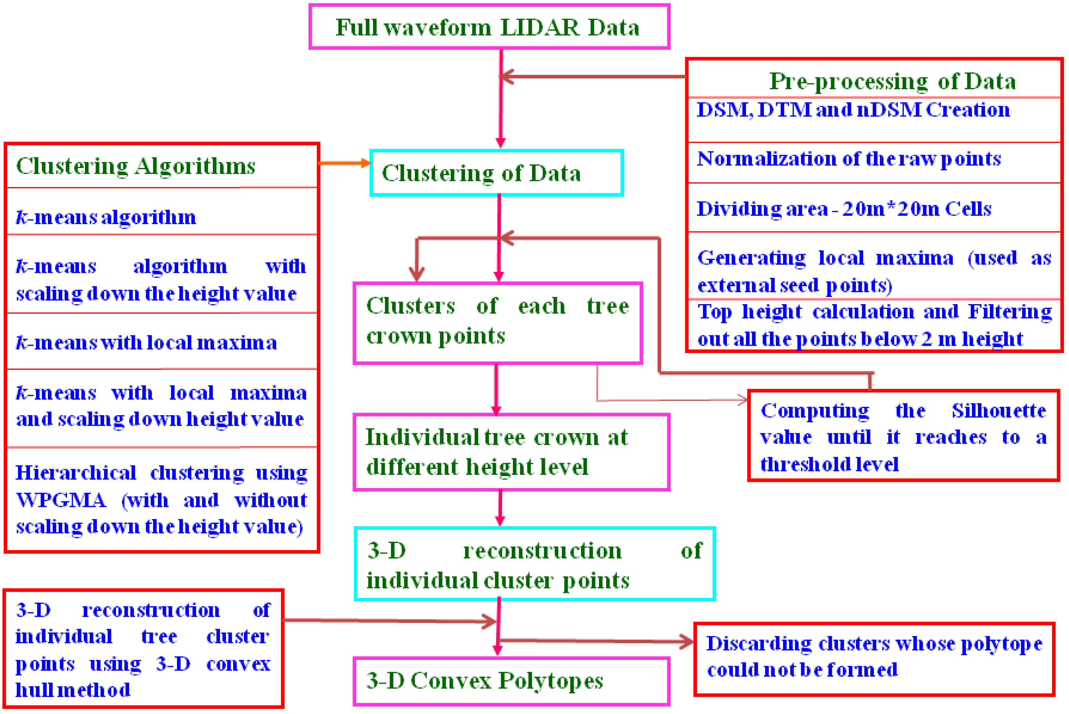
2.2. Methodology Flow Chart

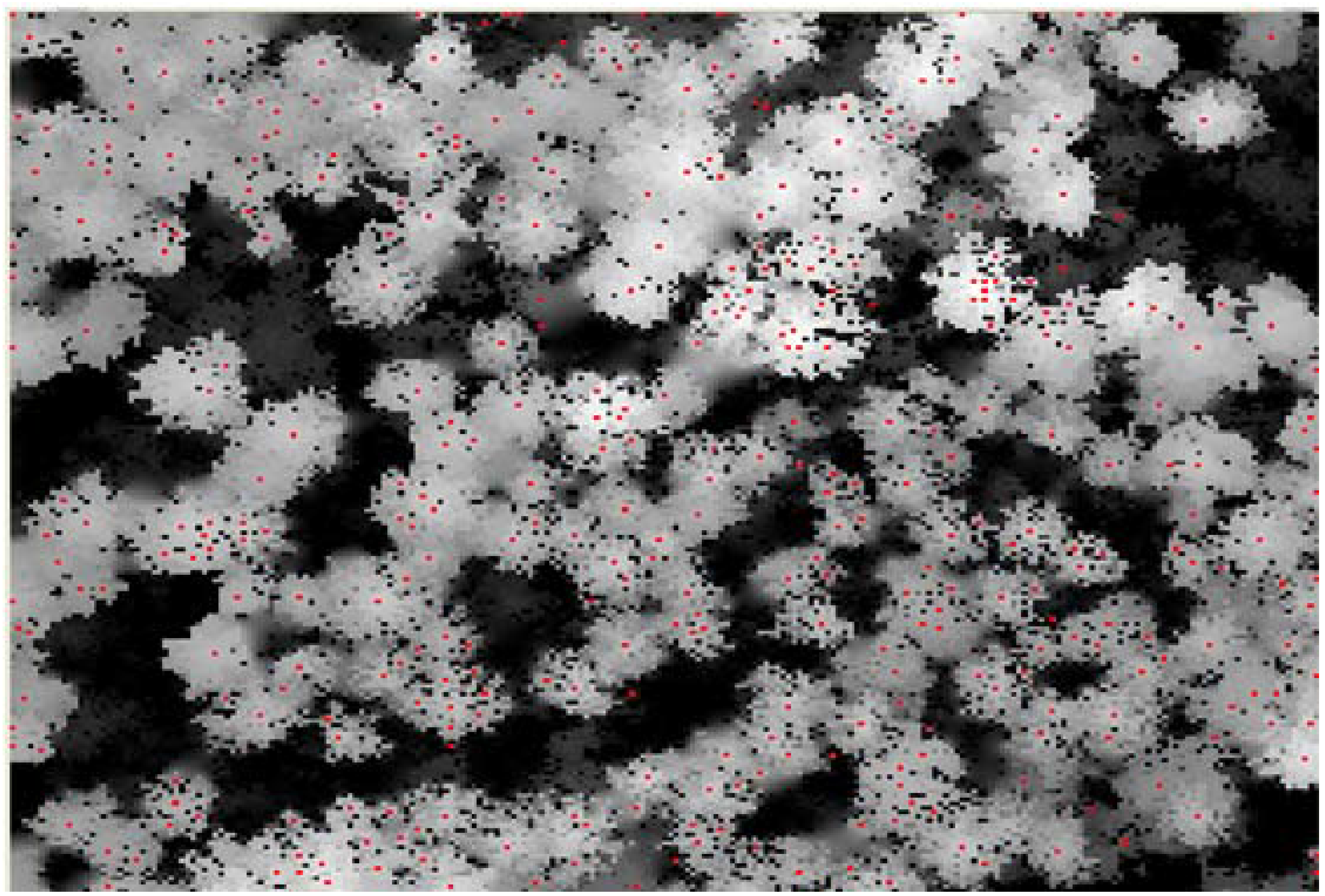
2.3. Generation of DSM, DTM and nDSM and Normalization of Raw LIDAR Data

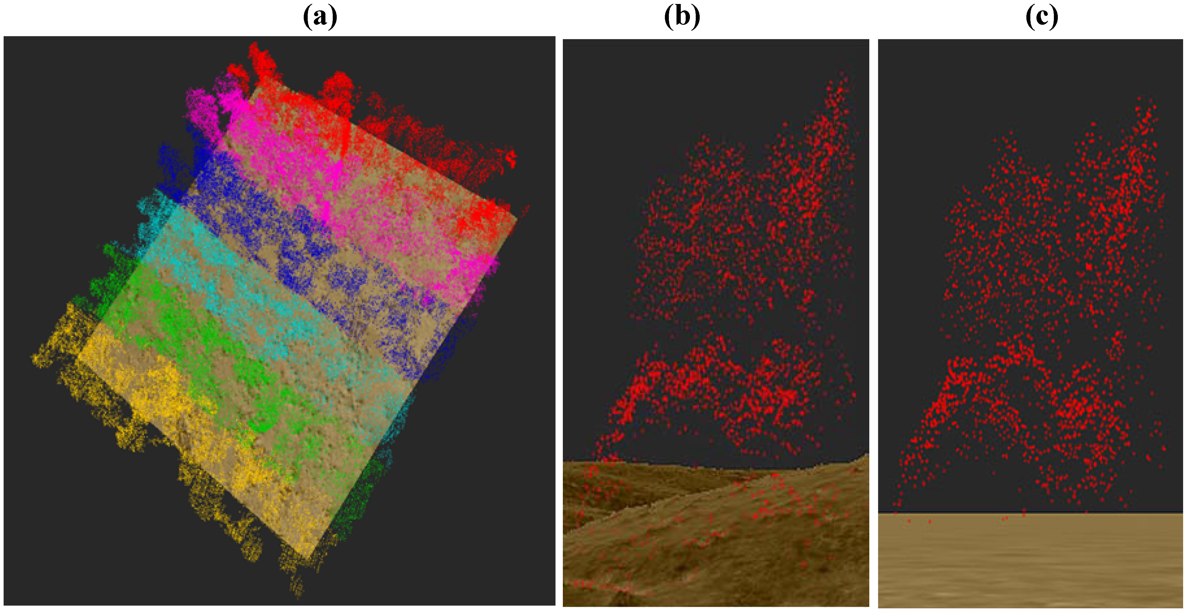
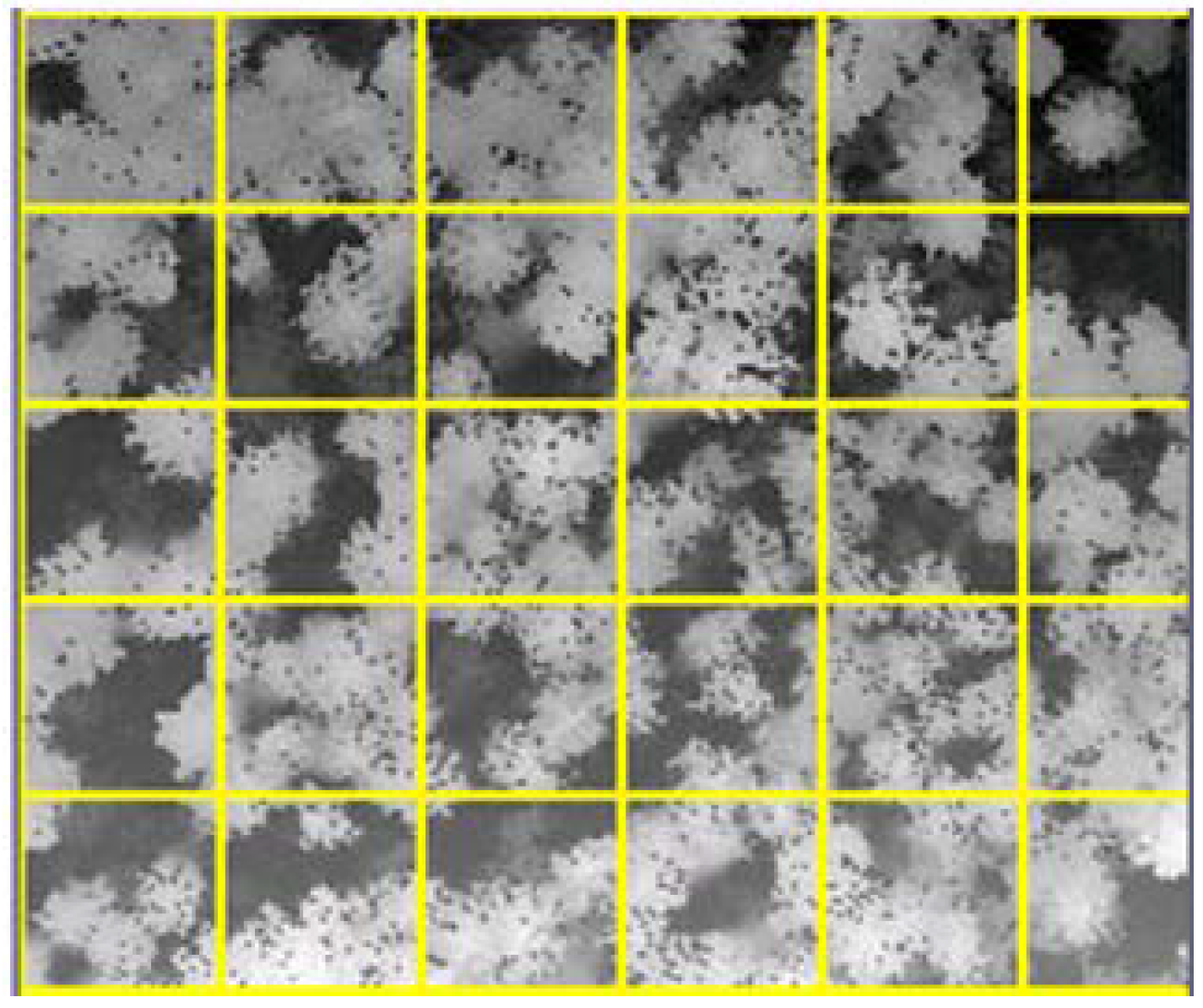
2.4. Study Area and Its Subdivision

| TopHeight [m] | |||||
|---|---|---|---|---|---|
| Cell1-39.79 | Cell2-42.78 | Cell3-44.89 | Cell4-49.73 | Cell5-47.47 | Cell6-38.17 |
| Cell7-39.35 | Cell8-40.41 | Cell9-46.01 | Cell10-51.57 | Cell11-50.63 | Cell12-41.64 |
| Cell13-39.31 | Cell14-41.23 | Cell15-44.58 | Cell16-43.72 | Cell17-39.54 | Cell18-39.32 |
| Cell19-37.27 | Cell20-39.96 | Cell21-41.02 | Cell22-39.30 | Cell23-39.39 | Cell24-39.38 |
| Cell25-37.92 | Cell26-43.23 | Cell27-41.98 | Cell28-40.5 | Cell29-38.45 | Cell30-37.14 |
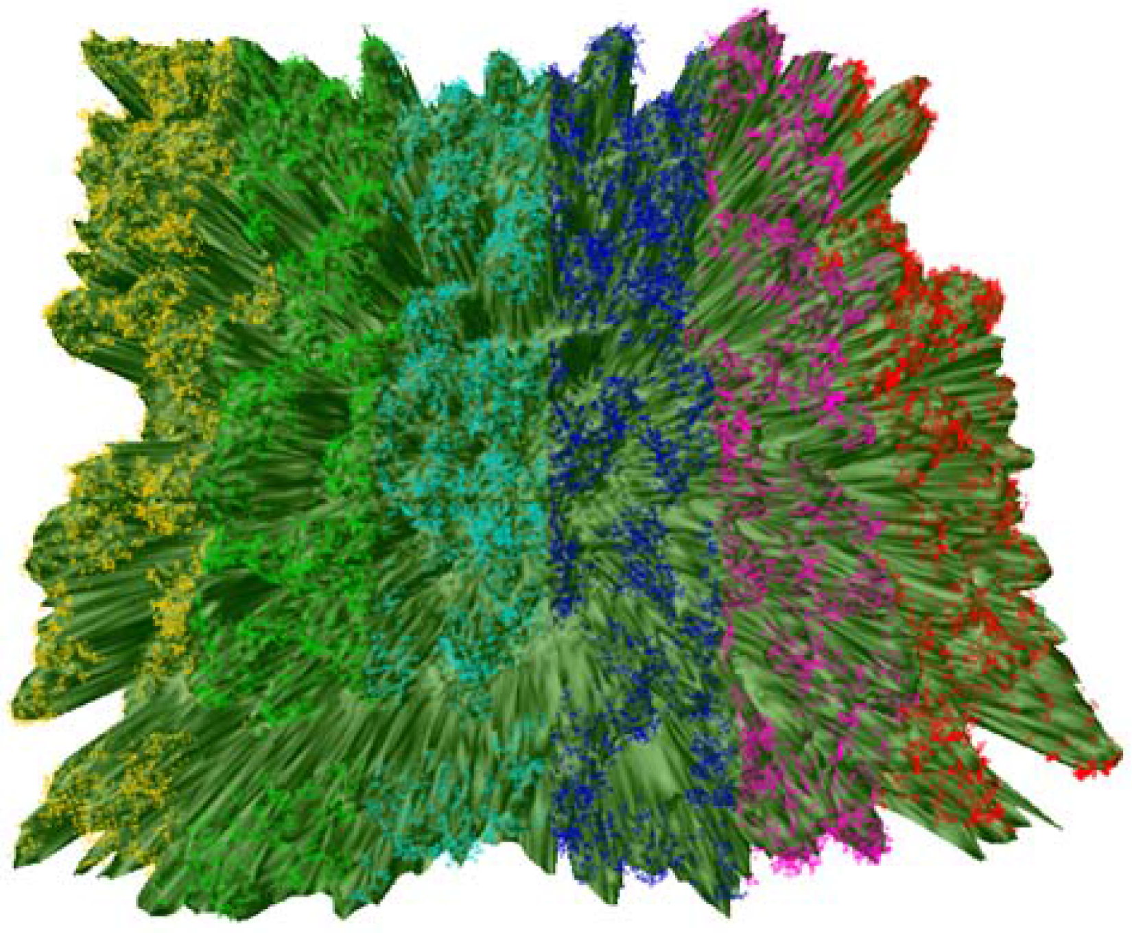
2.5. Clustering
2.5.1. Iterative Partitioning

2.5.2. Hierarchical Tree Method
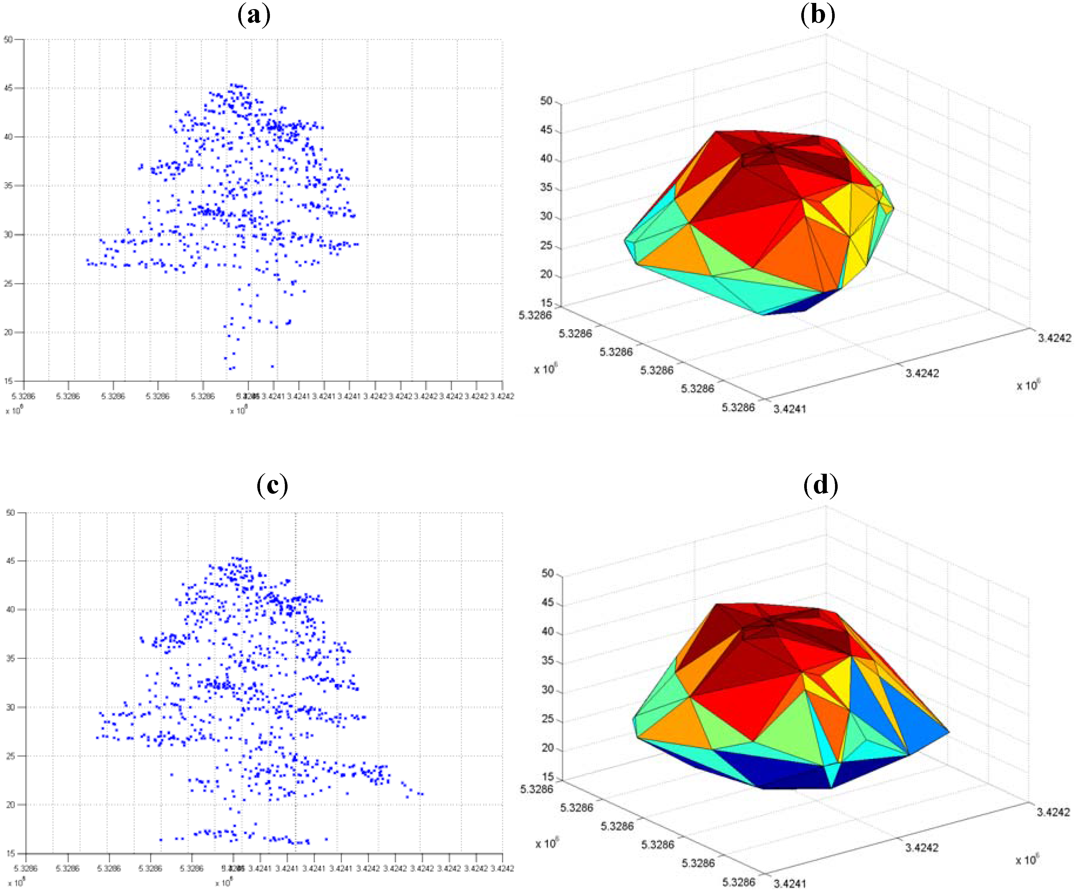
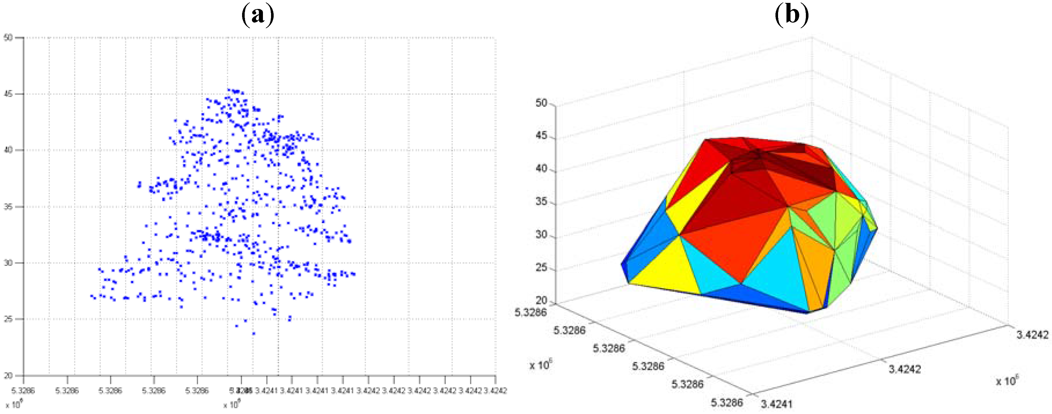
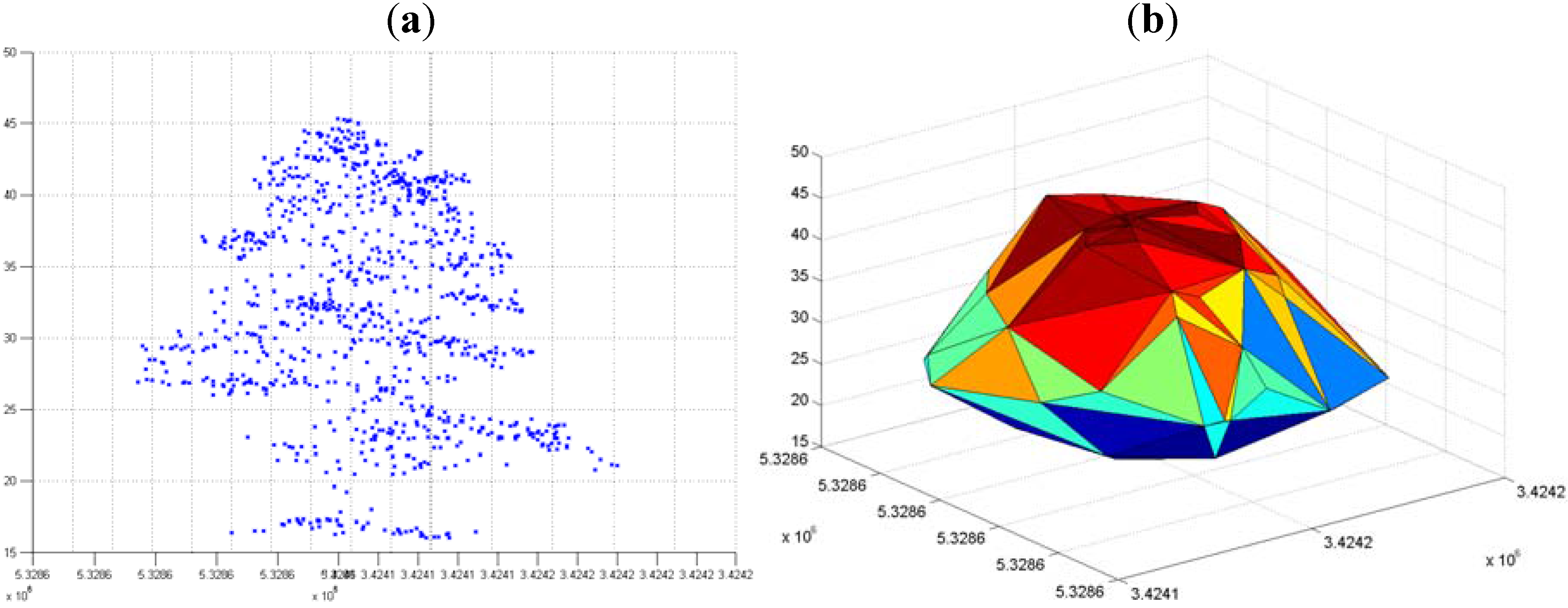
2.6. 3-D Reconstruction of Individual Tree Clusters
3. Results and Discussion

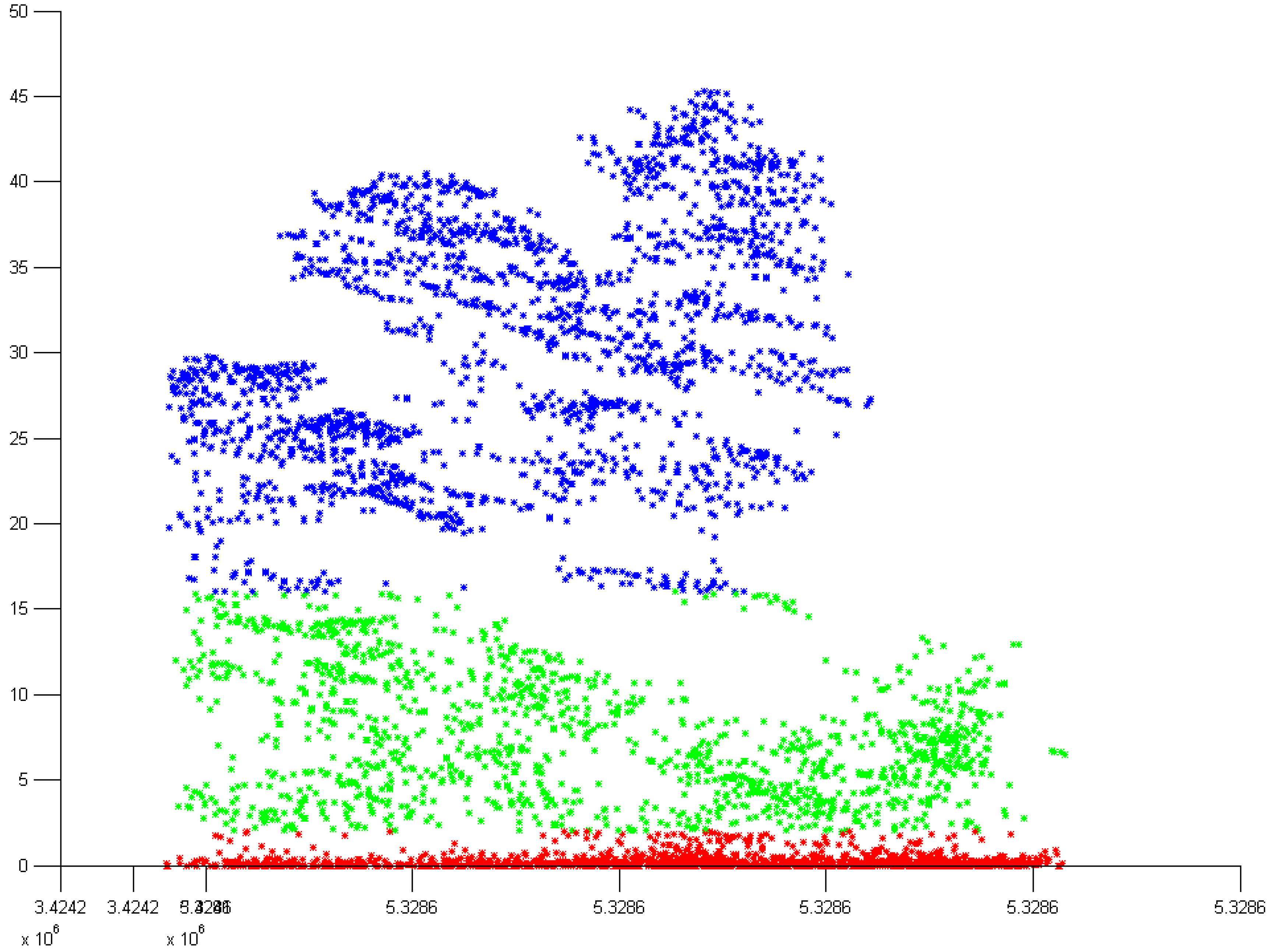
3.1. Normal k-means (N k-means)
3.1.1. Without Scaling Down the Height Value

3.1.2. By Scaling Down the Height Value


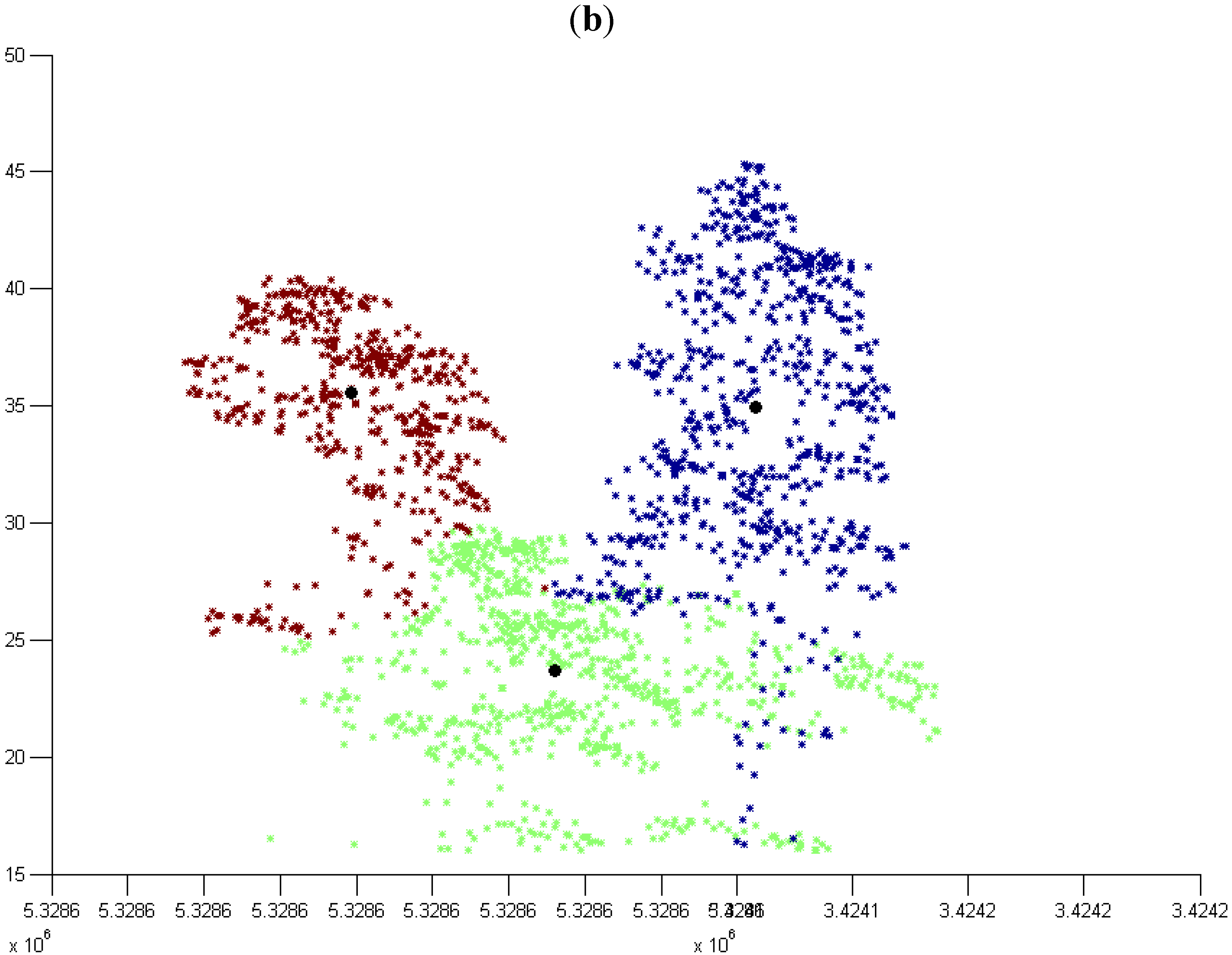
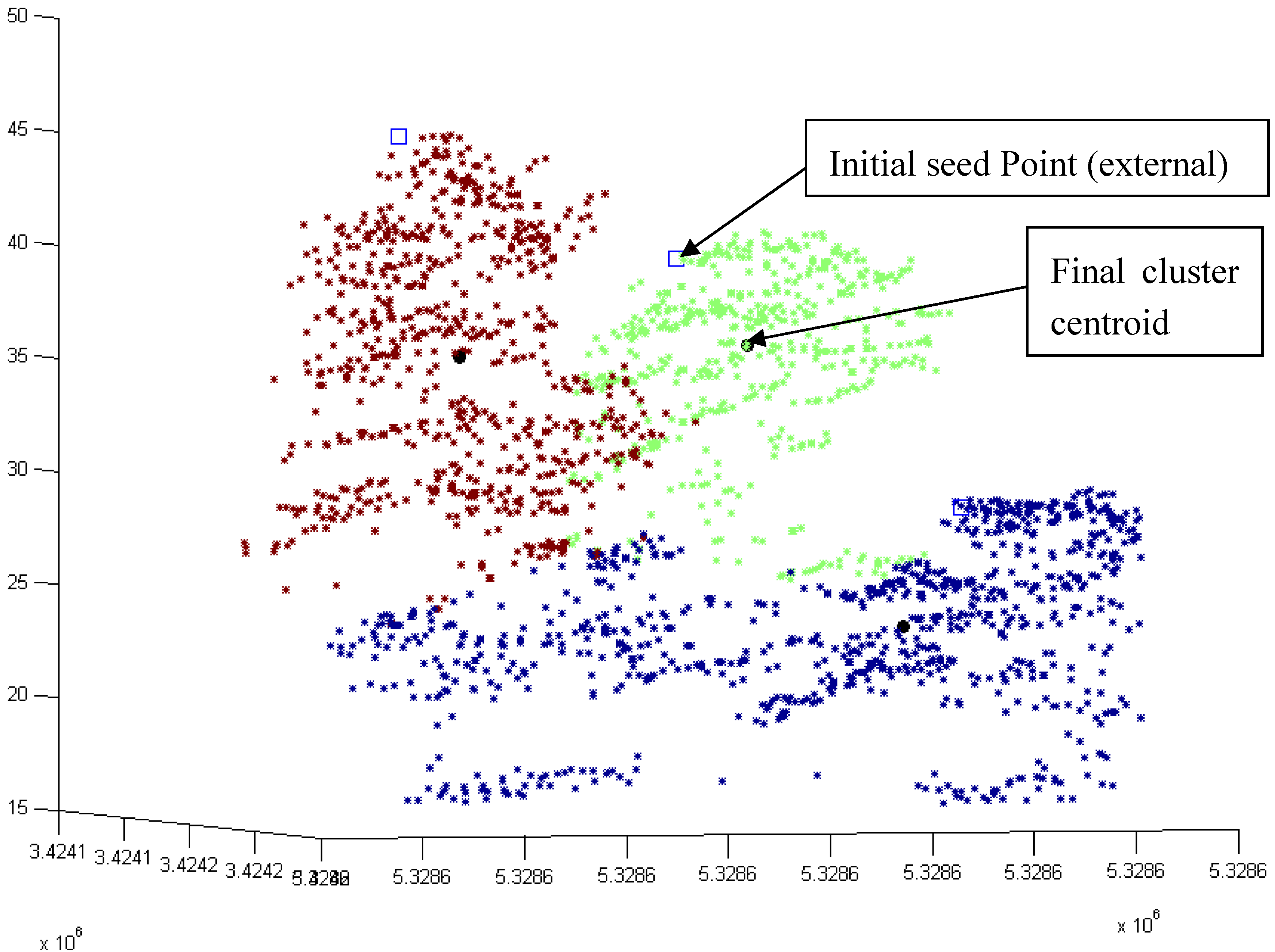
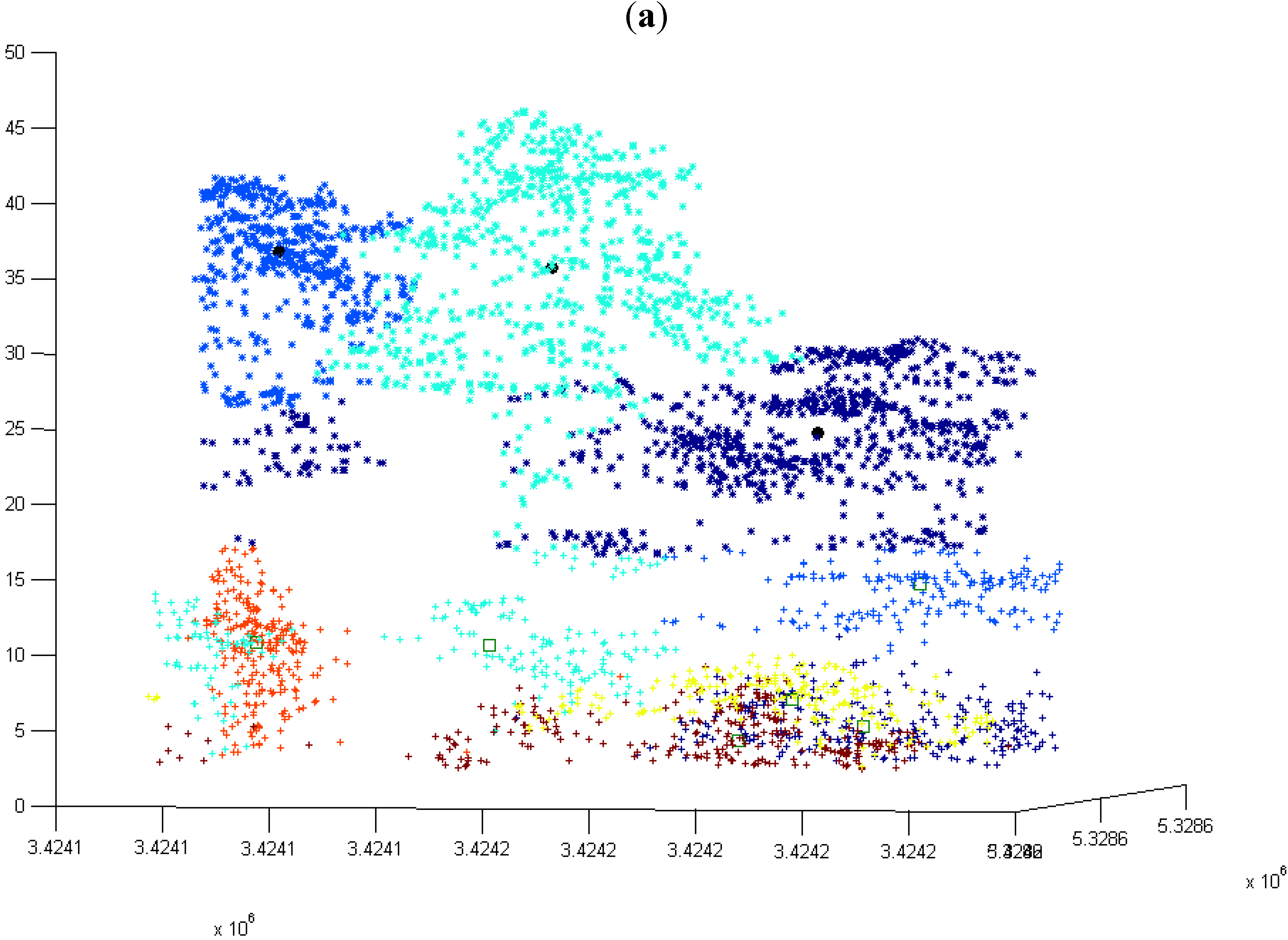
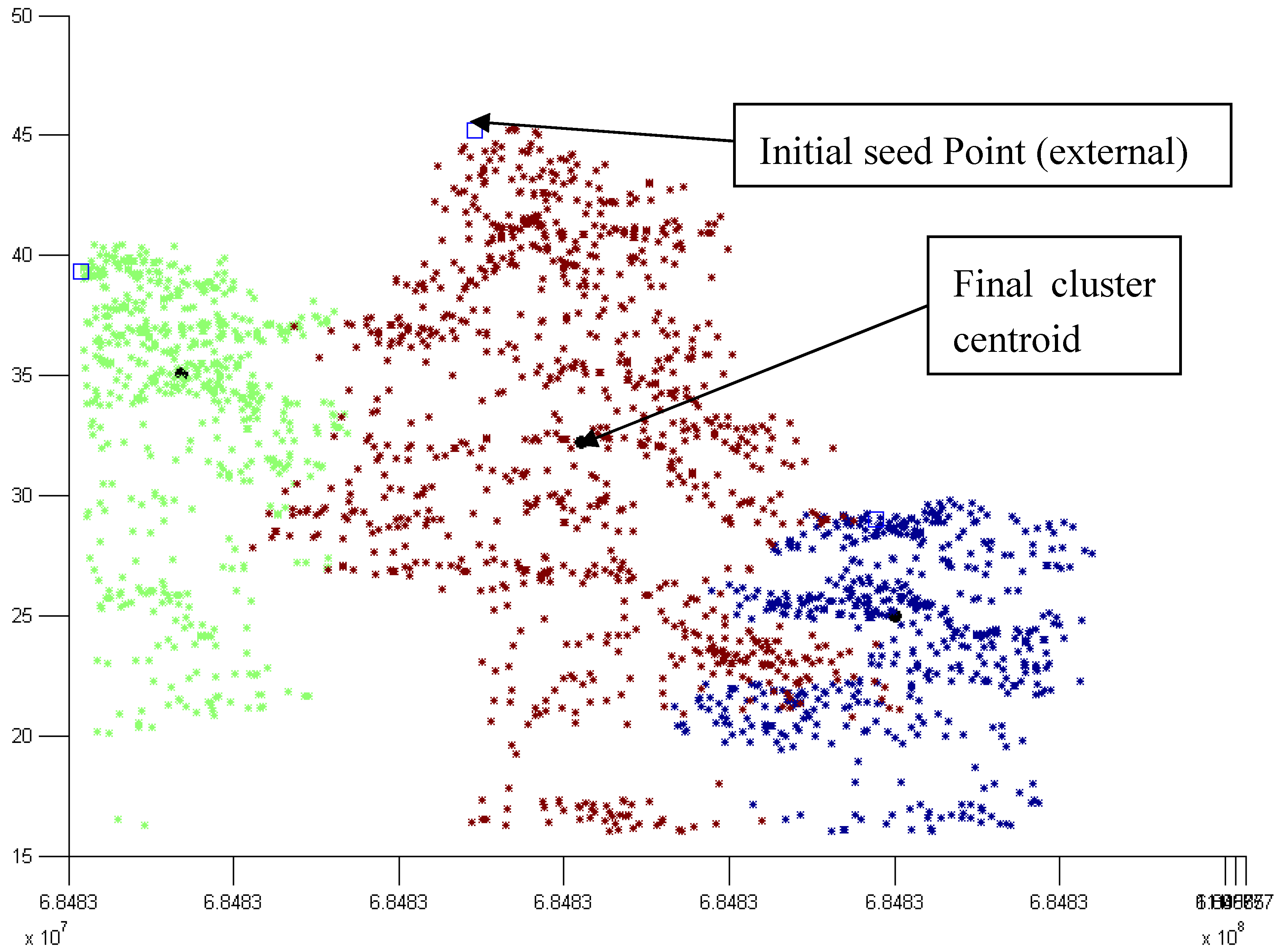
3.2. Modified k-means (M k-means) with External Seed Points
3.2.1. Without Scaling Down the Height Value

3.2.2. By Scaling Down the Height Value

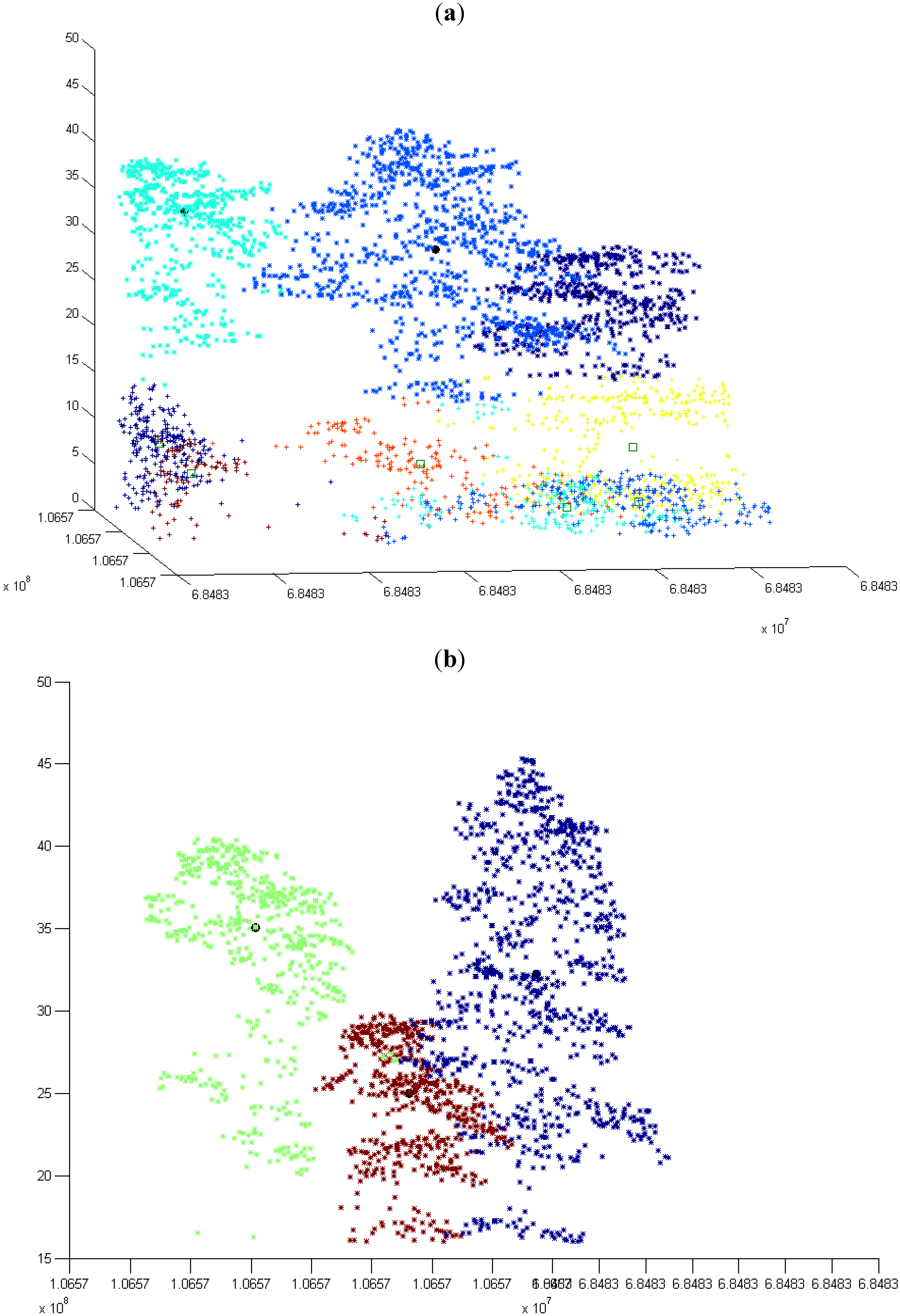
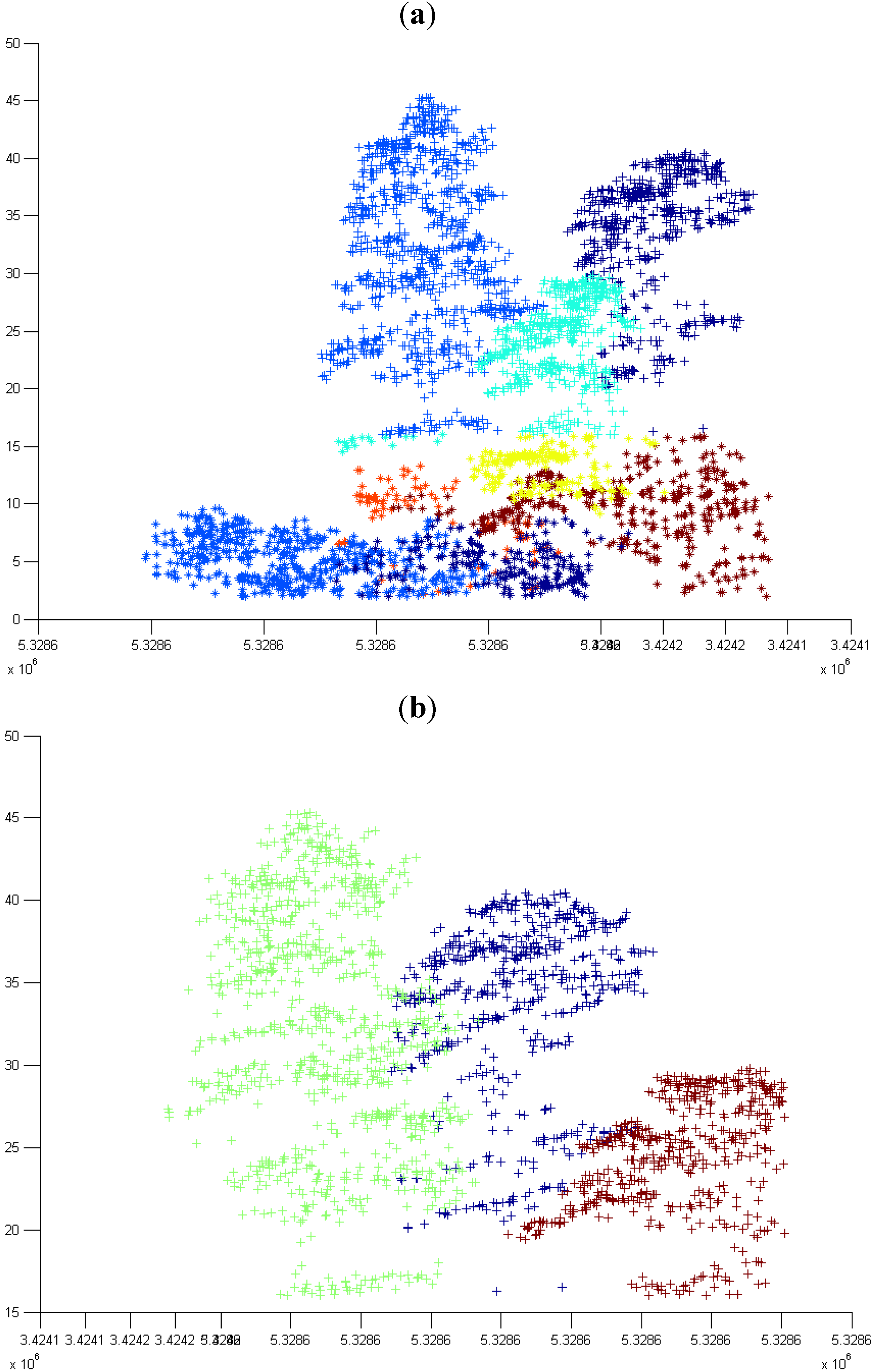
3.3. Hierarchical Tree Based Approach Using WPGMA Algorithm
3.3.1. Without Scaling Down the Height Value

3.3.2. By Scaling Down the Height Value
3.4. Number of Trees in All the Grids at the First Height Level
| Number of trees in each cell | |||||
|---|---|---|---|---|---|
| Cell 1-14 | Cell 2-16 | Cell 3-13 | Cell 4-15 | Cell 5-11 | Cell 6-3 |
| Cell 7-8 | Cell 8-7 | Cell 9-8 | Cell 10-24 | Cell 11-20 | Cell 12-5 |
| Cell 13-8 | Cell 14-12 | Cell 15-13 | Cell 16-13 | Cell 17-8 | Cell 18-9 |
| Cell 19-12 | Cell 20-15 | Cell 21-14 | Cell 22-13 | Cell 23-20 | Cell 24-16 |
| Cell 25-11 | Cell 26-20 | Cell 27-10 | Cell 28-19 | Cell 29-13 | Cell 30-8 |
4. Conclusions
Acknowledgements
References and Notes
- Hyyppä, J.; Yu, X.; Hyyppä, H.; Maltamo, M. Methods of airborne laser scanning for forest information extraction. In Proceedings of the International Workshop on 3D Remote Sensing in Forestry, Vienna, Austria, February 2006; pp. 63–78.
- Persson, A.; Holmgren, J.; Söderman, U. Identification of tree species of individual trees by combining very high resolution laser data with multi-spectral images. In Proceedings of the International Workshop on 3D Remote Sensing in Forestry, Vienna, Austria, February 2006; pp. 91–96.
- Wang, Y.; Weinacker, H.; Koch, B.; Krzysztof, S. Lidar point cloud based fully automatic 3d single tree modelling in forest and evaluations of the procedure. In Proceedings of the 21st ISPRS Congress, Vol. 37, Part B6b. Beijing, China, July 2008; pp. 45–52.
- Vauhkonen, J.; Tokola, T.; Packalén, P.; Maltamo, M. Identification of Scandinavian commercial species of individual trees from airborne laser scanning data using alpha shape metrics. For. Science 2009, 55, 37–47. [Google Scholar]
- Hyyppä, J.; Inkinen, M. Detecting and estimating attributes for single trees using laser scanner. Photogramm. J. Fin. 1999, 16, 27–42. [Google Scholar]
- Persson, A.; Holmgren, J.; Söderman, U. Detecting and measuring individual trees using an airborne laser scanner. Photogramm. Eng. Remote Sens. 2002, 68, 925–932. [Google Scholar]
- Koch, B.; Heyder, U.; Weinacker, H. Detection of individual tree crowns in airborne lidar data. Photogramm. Eng. Remote Sens. 2006, 72, 357–363. [Google Scholar] [CrossRef]
- Pyysalo, U.; Hyyppä, H. Reconstructing tree crowns from laser scanner data for feature extraction. In Proceedings of the ISPRS Technical Commission III Symposium for Photogrammetric Computer Vision, Graz, Austria, September 2002; pp. 293–296.
- Reitberger, J.; Krzystek, P.; Stilla, U. 3D segmentation and classification of single trees with full waveform LIDAR data. In Proceedings of SilviLaser 2008, Edinburgh, UK, September 2008; pp. 216–226.
- Morsdorf, F.; Meier, E.; Allgöwer, B.; Nüesch, D. Clustering in airborne laser scanning raw data for segmentation of single trees. In Proceedings of the ISPRS Working Group III/3 Workshop for 3-D Reconstruction from Airborne LaserScanner and InSAR Data, Dresden, Germany, October 2003; pp. 27–33.
- Morsdorf, F.; Meier, E.; Kötz, B.; Itten, K.I. Lidar based geometric reconstruction of boreal type forest stands at single tree level for forest and wildland fire management. Remote Sens. Environ. 2004, 92, 353–362. [Google Scholar] [CrossRef]
- Cici, A.; Kevin, T.; Nicholas, J.T.; Sarah, S.; Jörg, K. Extraction of vegetation for topographic mapping from full-waveform airborne laser scanning data. In Proceedings of SilviLaser 2008, Edinburgh, UK, September 2008; pp. 343–353.
- Doo-Ahn, K.; Woo-Kyun, L.; Hyun-Kook, C. Estimation of effective plant area index using LiDAR data in forest of South Korea. In Proceedings of SilviLaser 2008, Edinburgh, UK, September 2008; pp. 237–246.
- Ko, C.; Sohn, G.; Remmel, T.K. Classification for deciduous and coniferous trees using airborne lidar and internal structure reconstructions. In Proceedings of SilviLaser 2009, College Station, TX, USA, October 2009; pp. 36–45.
- Ørka, H.O.; Næsset, E.; Bollandsas, O.M. Comparing classification strategies for tree species recognition using airborne laser scanner data. In Proceedings of SilviLaser 2009, College Station, TX, USA, October 2009; pp. 46–53.
- Rieger, P.; Ullrich, A.; Reichert, R. Laser scanners with echo digitization for full waveform analysis. In Proceedings of the International Workshop on 3D Remote Sensing in Forestry, Vienna, Austria, February 2006; pp. 204–210.
- Hug, C.; Ullrich, A.; Grimm, A. LiteMapper-5600—A waveform-digitizing LIDAR terrain and vegetation mapping system. In Proceedings of ISPRS Working Group on Laser-Scanners for Forest and Landscape Assessment–Instruments, Processing Methods and Applications, Freiburg, Germany, October 2004; pp. 24–29.
- Weinacker, H.; Koch, B.; Heyder, U.; Weiancker, R. Development of filtering, segmentation and modelling modules for lidar and multispectral data as a fundament of an automatic forest inventory system. In Proceedings of ISPRS Working Group on Laser-Scanners for Forest and Landscape Assessment–Instruments, Processing Methods and Applications, Freiburg, Germany, October 2004; pp. 50–55.
- Burschel, P.; Huss, J. In Grundriss des Waldbaus, 1st ed.; Eugen Ulmer Verlag: Parey Text Series, Berlin, Germany, 1997; pp. 67–68. [Google Scholar]
- Sneath, P.H.A.; Sokal, R.R. In Numerical Taxonomy: The Principles and Practice of Numerical Classification, 2nd ed.; W.H. Freeman and Company: San Francisco, CA, USA, 1973. [Google Scholar]
- Barber, C.B.; Dobkin, D.P.; Huhdanpaa, H.T. The Quickhull algorithm for convex hulls. ACM Trans. Math. Software 1996, 22, 469–483. [Google Scholar] [CrossRef]
- Berg, M.D.; Kreveld, M.V.; Overmars, M.; Schwarzkopf, O. Convex Hulls—Mixing Things. In Computational Geometry—Algorithms and Applications; Springer-Verlag: Berlin, Heidelberg, Germany, 1997; pp. 233–248. [Google Scholar]
© 2010 by the authors; licensee Molecular Diversity Preservation International, Basel, Switzerland. This article is an open-access article distributed under the terms and conditions of the Creative Commons Attribution license (http://creativecommons.org/licenses/by/3.0/).
Share and Cite
Gupta, S.; Weinacker, H.; Koch, B. Comparative Analysis of Clustering-Based Approaches for 3-D Single Tree Detection Using Airborne Fullwave Lidar Data. Remote Sens. 2010, 2, 968-989. https://doi.org/10.3390/rs2040968
Gupta S, Weinacker H, Koch B. Comparative Analysis of Clustering-Based Approaches for 3-D Single Tree Detection Using Airborne Fullwave Lidar Data. Remote Sensing. 2010; 2(4):968-989. https://doi.org/10.3390/rs2040968
Chicago/Turabian StyleGupta, Sandeep, Holger Weinacker, and Barbara Koch. 2010. "Comparative Analysis of Clustering-Based Approaches for 3-D Single Tree Detection Using Airborne Fullwave Lidar Data" Remote Sensing 2, no. 4: 968-989. https://doi.org/10.3390/rs2040968