Estimating Speed and Direction of Small Dynamic Targets through Optical Satellite Imaging

Abstract

Moving Target Indicators (MTI) are systems used to distinguish movement from stationary scenes and sometimes to derive the spatial attributes of these objects. These systems are currently used in many sectors such as traffic studies, border surveillance, and military applications. The proposed MTI reveals vehicles and their velocities using commercial imagery from a passive optical satellite-mounted sensor. With simple process of image differencing, the MTI can automatically recognize conveyances in motion (speed and direction) represented by polygons formed by a group of pixels from successive images. Micro-change detection with an existing commercial satellite requires special considerations of differences in spatial and spectral resolution between images. Complications involving the movement detection system such as vehicle overlap, vehicle clusters, and zones of low confidence are refined by adding error-reducing modules. This process is tested on a variety of vehicles, their concentrations, and environments, confirming the feasibility of utilizing an MTI with commercial optical satellite imagery for movement recognition and velocity estimation.

1. Introduction

A Moving Target Indicator (MTI) is defined as a system able to distinguish movement from a background and compile the spatial attributes of these moving objects. RADAR, LiDAR, aerial photography, and film sequences are common media for MTIs. MTIs employing Synthetic Aperture RADAR (SAR) imagery are used in the commercial sector for detecting ice movement, deforestation tracking, and border surveillance [1]. Military applications involve MTIs to gain knowledge of the enemy [2] by recognizing and tracking hostile force movements, deployment patterns, and supply histories.

Groups involved in the recent conflicts in the Middle East have employed the QuickBird sensor for wide-area surveillance of the battlefield. QuickBird and other commercial optical sensors may be a medium through which ground vehicles in motion can be identified using an MTI. The purpose of this research was to design and test an MTI that uses the high-resolution commercially-available satellite imagery to return possible moving targets, such as planes, small autos, and tractor-trailers. The size, speed, and direction of ground targets, can be collected automatically from a variety of terrain types.

With the large collection swath of current commercial satellites, an MTI that can automatically flag moving formations or single vehicles in an area of 10,000 square kilometers of isolated, perhaps dangerous terrain has obvious benefits. Flight habits of suspicious low-altitude aircraft in isolated environments like the Florida Everglades could be revealed using this method. Air-zone restrictions are not extended to satellites and “no-fly” designated zones due to political concerns and hostile responses can be frequently studied using imagery from space-based sensors. While an MTI that uses optical satellite images has some definite advantages, there are currently limitations on such systems, including limited ground separation distances (GSD), revisit times, and radiometric energy requirements.

Recognizing movement from some optical satellite imagery is possible through minor delays between the acquisition of the panchromatic and multi-spectral images. The Dynamic Offset of Targets (DOTs) represents the direction and speed recognizable in pan-sharpened images. The spatio-temporal characteristics of these DOTs can be automatically derived using the temporal shift of the sensor’s panchromatic and the multi-spectral bands. This project focuses not on multiple, ultra resolution images obtained from low-altitude aircrafts or ground-based cameras, but rather on satellite-borne bi-resolution scenes where a vehicle may be represented by a few pixels.

After modifying the MTI to a configuration of greater accuracy, these techniques were tested on automobiles and aircraft and the results posted. Different environments and their effects yield some valuable information regarding the limitations of such an MTI. The size, speed, and direction are automatically collected from autos and aircraft occupying a variety of terrain types, such as cityscapes and arid environments. Issues with the MTI are described and techniques for enhancing the system are introduced.

2. Related Studies

Micro-change technology is not a new science for locating and tracking vehicles, only the medium through which it may be accomplished. A number of studies involve the use of sensors, such as aircraft, human being, automobiles, and missiles.

MTIs use data from fixed ground sensors, aerial sensors, and periodically revisiting sensors such as orbiting satellites. High-resolution aerial photography has been extensively studied in recent years for a possible solution to manual traffic counts and other traffic-flow related topics [3,4,5]. Some MTIs use video sequences or multiple, high-resolution images of a single view. Thresholding, a form of image segmentation, separates movement and non-movement in this MTI. Matching refers to the process of attaching a physical shape to each moving target and tracking this shape through successive frames [6,7,8]. For example, an automobile appearing in ultra resolution imagery might be “segmented” into several areas according to a specific range of digital numbers: roof, trunk, hood, windshield, and accompanying cast shadow. This in-depth segmentation is often used with extremely high spatial resolution (< 0.5 meter) datasets.

Problems with previous MTI sensors include the limited availability of timely sensor coverage, the lack of wide-area, high-resolution imagery, and the inability to discriminate between moving vehicles of differing types [2]. These limitations have been reduced somewhat by the Synthetic-Aperture RADAR (SAR) MTI sensors.

MTIs using SAR can detect small-pixel count objects in low-resolution environments. The targets in motion are identified through conventional methods using the Doppler shifts of moving targets [9,10] and by others employing a passive system of image differencing to create a relief of movement. Image difference methods have proven consistent in flagging movement in both SAR and imagery from an airborne platform [3,11]. When determining the difference between two scenes, the stationary components of both should cancel, leaving a value near zero.

The goal of this project is to evaluate the functionality of the developed method for high-resolution space-borne sensors; not limited to the imagery used as increasing governmental allowances for commercial resolutions are expected. Some errors associated with the proposed MTI will decrease with each increasing resolution allowance. Thus, the project focused on verifying this method of movement recognition using differing spatial and spectral resolution images and not specifically on the imagery provided by the QuickBird sensor.

3. Optical Satellite MTI Methodology

QuickBird captures a panchromatic image first followed by collection of the lower-resolution multi-spectral image following 0.2 seconds later. The brief lapse in time between the retrieval of these two images provides information about object’s spatio-temporal characteristics. An MTI then exploits the small changes that occur in that narrow time gap allowing a reasonable estimate of speed and bearing using time-distance equations.

3.1. Data Description

This study used QuickBird standard imagery from DigitalGlobe, Inc. QuickBird provides 0.61–0.72 meter resolutions for the panchromatic and 2.44–2.88 meters for its multi-spectral imagery, depending on the maximum off-nadir view angle. As the sensor’s look angle increases, the distance between it and the area of interest lengthens, reducing spatial resolutions. DigitalGlobe grades image quality on a scale from 1 to 100 with corresponding terms like “poor” (20), “fair” (50), and “excellent” (90). These classes are derived from cloud cover, environmental quality, and a predicted value (PNIIRS) guided by the National Imagery Interpretability Rating Scale. This scale is used as a guide to quantify the overall usability of optical imagery according to radiometric environment, sensor quality, and illumination. Table 1 displays the spectral bandwidth of the panchromatic and multi-spectral bands.

Table 1. Spectral ranges of the QuickBird sensor.

Spectral Band	Bandwidth (ηm)
Panchromatic	450–900
Blue (channel 1)	450–520
Green (channel 2)	520–600
Red (channel 3)	630–690
Infrared (channel 4)	760–900

Table 1. Spectral ranges of the QuickBird sensor.

Spectral Band	Bandwidth (ηm)
Panchromatic	450–900
Blue (channel 1)	450–520
Green (channel 2)	520–600
Red (channel 3)	630–690
Infrared (channel 4)	760–900

3.2. Data Preparation

Raw optical satellite imagery must be modified so that the data is suitable for viewing and interpreting before processing it within an MTI. Standard imagery arrives geometrically and radiometrically corrected including amendments for noise.

Images of the same area collected at various times are inherently different from one another. Satellite flight path, look angle (both across and in-track), the angle of the sun, the distance between the earth and the sun, and atmospheric conditions are all factors in the spectral response of the study area [12,13]. Due to the geometry of the collection swath and the sensor’s orbit, cell-size variations are expected within ±0.2 cm. This means that cells near the edges of the scene will have slightly lower spatial resolution. For example, one cell collected with this satellite at nadir may have an x and y resolution of 0.61 meters. A cell collected one-hundred kilometers from this point of maximum accuracy should have an x resolution of 0.615 meters and a y resolution of 0.630 meters. Standard imagery is corrected for this panoramic distortion [14].

The multi-spectral (MS) and pan-chromatic (PAN) images are not co-registered. For the two images to properly align without requiring additional co-referencing it is assumed that row and column uncertainty for the dataset must be relatively low and image quality high. The row and column uncertainties reflect the uncertainty of the corners in meters [14]. It is crucial to maintain geospatial alignment as one pixel can introduce significant error in the determination of object motion and speed. Entire travel lanes can appear shifted when comparing the panchromatic imagery to the multi-spectral imagery. The mitigation of the geo-referencing errors by co-rectification is mostly subjective and might introduce even more error. Xiong and Zhang [15,16] have investigated methods to reduce the error attributed to image scale, ground relief, and image resampling for vehicle extraction from high-resolution satellite imagery.

The images were re-sampled using cubic convolution to create a display matrix from the original collected matrix. Resampling involves substituting corrected coordinates for pixels to remove distortion. Unlike the other methods, the cubic convolution reduces spatial error and returns shaper images; however, in the smoothing process, it can lose some contrast.

3.3. Sequential Frame Building

Spectral similarity must be maintained between the two datasets, panchromatic and multi-spectral, for an MTI to properly recognize change. Some similarity can be achieved by creating a synthetic PAN image using the bands in a MS image. A weighted algorithm was applied to the MS image to create a synthetic PAN image (Equation 1). The digital numbers of each band are weighted and then combined to yield one digital number for each pixel and a one-band simulated PAN image.

$$\mathrm{Synthetic}\mathrm{Panchromatic}=D{N}_{Blue}*\frac{70}{350}+D{N}_{Green}*\frac{80}{350}+D{N}_{\mathrm{Re}d}*\frac{60}{350}+D{N}_{Infraed}*\frac{140}{350}$$

(1)

The resulting simulated pan closely resembles the original pan chromatic image, but maintains its original GSD. In addition, the spectral resolution of the panchromatic band is not matched in its entirety by the range of the MS bands (Table 1). The discrete nature of the multispectral image’s bandwidth will create problems. Band widths 600–630 and 690–760 ηm are absent from the multispectral bands so during calculations, a maximum pixel value difference of 100 is expected for like areas. The actual value of these spectral discontinuities may elude close estimation so this error may be irreducible. The following section contains one option.

3.4. Recognize Movement

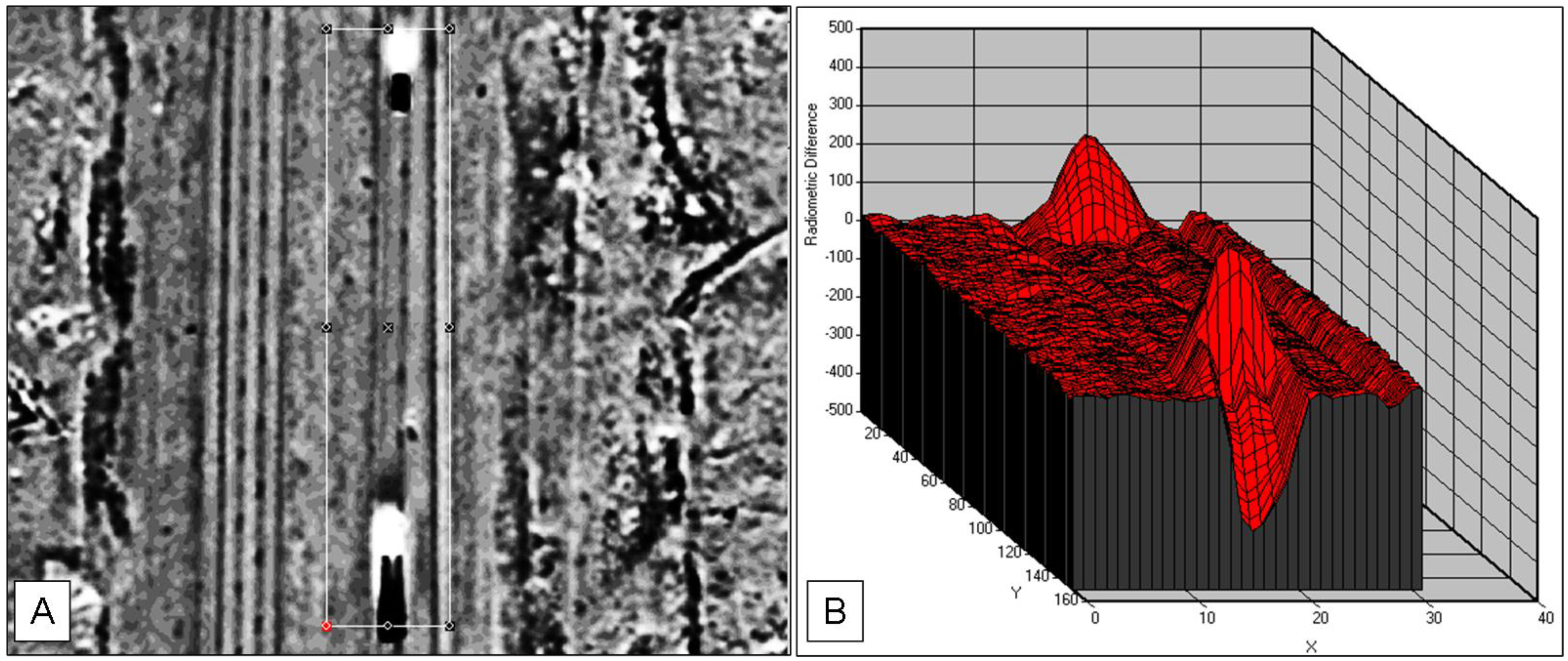
The two images, panchromatic and synthetic pan, act as two frames. After performing image differencing, it is possible to see the distance traveled within a set amount of time. The sensor collects the panchromatic image before the multispectral so when the former is subtracted from the latter, one can view the pixel changes representing the forward progress of moving objects. After subtracting the two images, the pixel value differences are reported and the temporal spatial change determined. A threshold allows the user to define the range of pixel values differences to be returned. Thresholding segregates imagery by criteria, in this case sufficient pixel value differences to classify as movement. One can discount the lower pixel value changes as remnants of minor shifting due to small rectification errors, spectral discontinuities, and other forms of noise (Figure 1).

Adaptive filtering (Equation 2) of the difference image can sometimes yield fewer false-positives. Filtering in this manner “stretches” the image to strengthen the contrast between objects, allowing greater separation for the user when choosing threshold values. The contrast multiplier sets the degree of contrast desired between nearby objects.

An indicator function separates pixels designated as movement and those designated as no movement (Equation 3). Thresholds were chosen for each study area and these varied from scene to scene to return the best ratio of confirmed movement and false-positives. The operator must discriminate between movement and non-movement. The threshold level is not static for each experiment, but tailored specifically to the image. If the upper limit is set too low, a user should expect to capture most moving targets at the expense of additional false-positives. If this threshold is set too high, the MTI may miss valid movement but will return less noise.

$$D{N}_{OUT}=K(D{N}_{Hi})+D{N}_{LL}$$

(2)

where:

• K = user selected contrast multiplier
• Hi = high luminance (derived from the lookup table)
• LL = local luminance (derived from the lookup table)

Figure 1. The difference in digital numbers for a highway segment containing two automobiles (a) with the movement of a passenger car and tractor trailer shown as spikes and valleys in contrast to the normal response (b).

Figure 1. The difference in digital numbers for a highway segment containing two automobiles (a) with the movement of a passenger car and tractor trailer shown as spikes and valleys in contrast to the normal response (b).

$$I\left(t:d\left(x,y\right)\right)=\begin{array}{cc}1& \left|d\left(x,y\right)\right|\ge t\\ 0& \left|d\left(x,y\right)\right|<t\end{array}$$

(3)

where:

• t = threshold
• d = difference in digital numbers between the two images
• 1 = movement
• 0 = no movement

Choosing a threshold is guided by many factors: the amount of variability in the landscape, the degree of elevation changes, land usage, size of search area, anticipated vehicles attributes (type, color, size), and the allowable false-positive to actual movement ratio. Placing the threshold to classify, for example, the upper and lower ten percent of a scene’s returned pixel value difference as movement, may be beneficial in an environment supporting frequent movement such as a highway. Thresholding in this manner may be a poor choice in an area where noise spikes are common, such as in an urban area or wooded region, because the excessive false-positive to actual movement ratio.

3.5. Recognizing and Tracking Vehicles

Once possible movement has been flagged, the portion of the PAN and simulated PAN images that represent movement are converted to polygons for vector calculations of rate of movement. A centroid matching process is then used to create movement pairs, which yields the bearing and speed of each vehicle.

Slower moving vehicles will return false velocities because of the overlap between images. These vehicles are slow and commonly will not completely escape their original spatial extent before the second image is collected. These movement polygons will show increased speed and decreased area from increased centroid-pair separation and overlap cancellation. The overlap requires additional polygon development if one was not willing to manually measure the distance traveled between acquisitions.

To reduce error, the polygons of each image, PAN and simulated PAN, were sieved using spatial constraints of area and elongation. The sieving process will vary according to the dimensions of the target vehicle. Allowable minimum and maximum areas of 3 to 45 m² were used for automobiles and tractor-trailers and 25 to 500 m² for a generic airplane search at most altitudes. Invalid linear movement-polygons tend to form alongside fabricated structures due to parallax and pixel mixing. 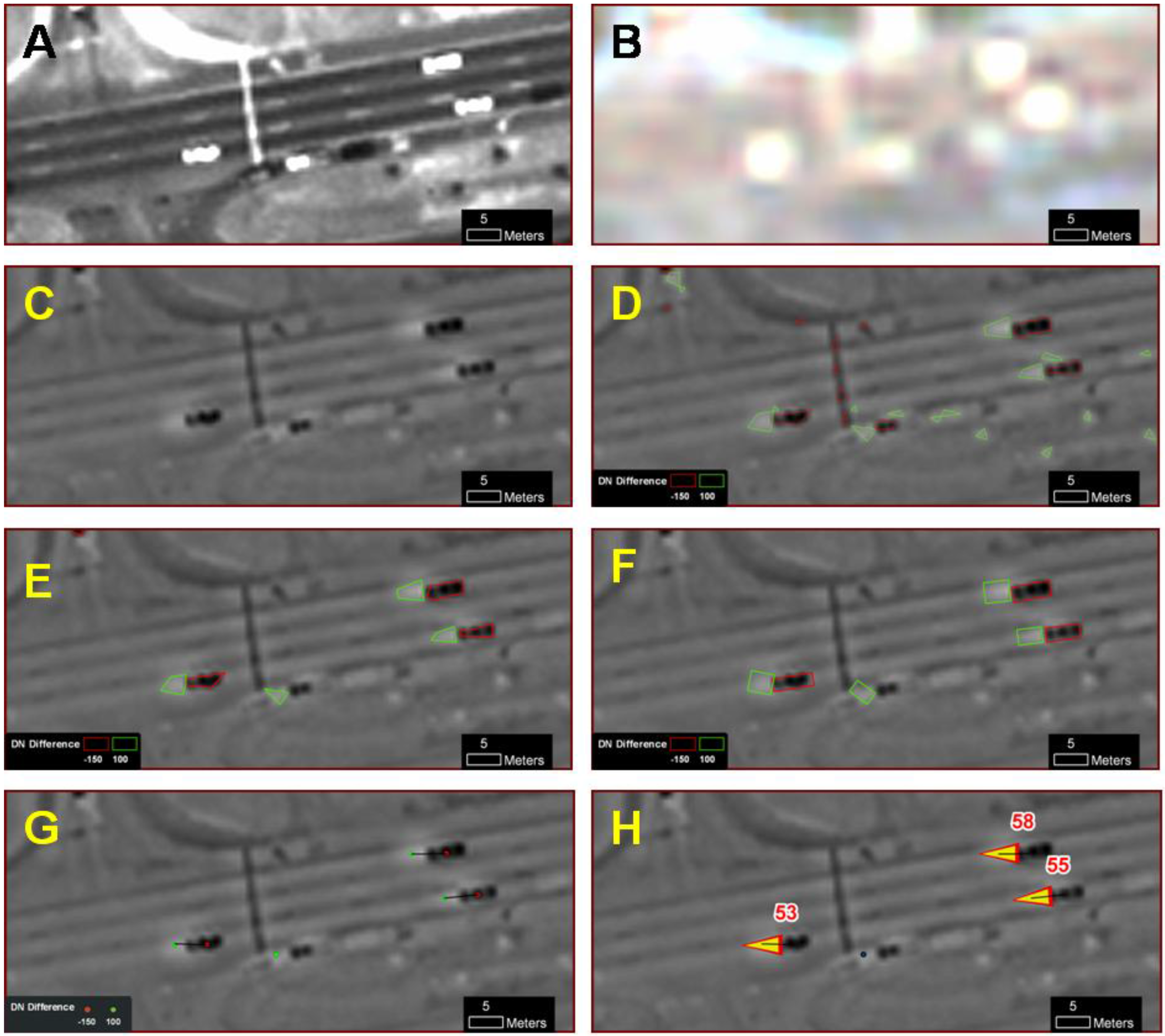Rotating bounding boxes constructed using a program prepared by Kuykendall [17] over the normally irregularly shaped polygons provide the length and width for elongation calculation (Figure 2F).

An accepted method of detecting moving vehicles is by the centroid or center point of a vehicle [18]. The coordinates for the polygon centroids provide an estimate of the initial and the final location (Figure 2G). The paired centroids represent a spatial-temporal shift described here as the Dynamic Offset of Target (DOT) (Figure 2H). Several constraints can be applied to pairing: proximity, or minimum distance, area and elongation of the parent polygons, mean DN of bounding refined polygon, variance of DNs within bounding box, and traffic morphology rules. An example of paring equation is shown below where polygon pair’s relative degree of relation is returned.

$$N=W_1\left({\sigma }_L-{\sigma }_{L+1}\right)+W_2\left({\mu }_L-{\mu }_{L+1}\right)+W_3\left(a_L-a_{L+1}\right)+W_4\left(E_L-E_{L+1}\right)+W_5\left(d\right)$$

(4)

where:

• N = relative degree of relation
• σ = standard deviation of pixel values within polygon
• µ = mean of pixel values within polygon
• a = area
• E = elongation (length to width ratio)
• d = separation distance between centroids
• W_n = user-defined weights

The user-defined weights in Equation 4, are used to calibrate the degree of relation between pairs of polygons based on environmental variables such as, spatial and spectral resolution of images, type of movement investigated, size of vehicles, land-cover characteristics, and others.

Figure 2. A panchromatic (a) and multispectral (b) segment of a road is subjected to image subtraction (c). Raster cells are converted to polygons representing initial and final locations (d) and then sieved by area (e). Bounding boxes used for sieving by elongation (f) to counter parallax and pixel mixing. The centroid of these polygons are paired for the movement vector (g) to determine the Dynamic Offset of Target for estimated speed in miles per hour (h).

Figure 2. A panchromatic (a) and multispectral (b) segment of a road is subjected to image subtraction (c). Raster cells are converted to polygons representing initial and final locations (d) and then sieved by area (e). Bounding boxes used for sieving by elongation (f) to counter parallax and pixel mixing. The centroid of these polygons are paired for the movement vector (g) to determine the Dynamic Offset of Target for estimated speed in miles per hour (h).

4. Selected Experiments

Tests of this MTI include varying data characteristics such as image quality, GSDs, and attributes specific to the vehicle type. For automobiles, these are environment types, contrast levels, and vehicle velocities, size, and concentrations. Aircraft in flight was tested using a rough estimate of altitude.

4.1. Automobile Detection

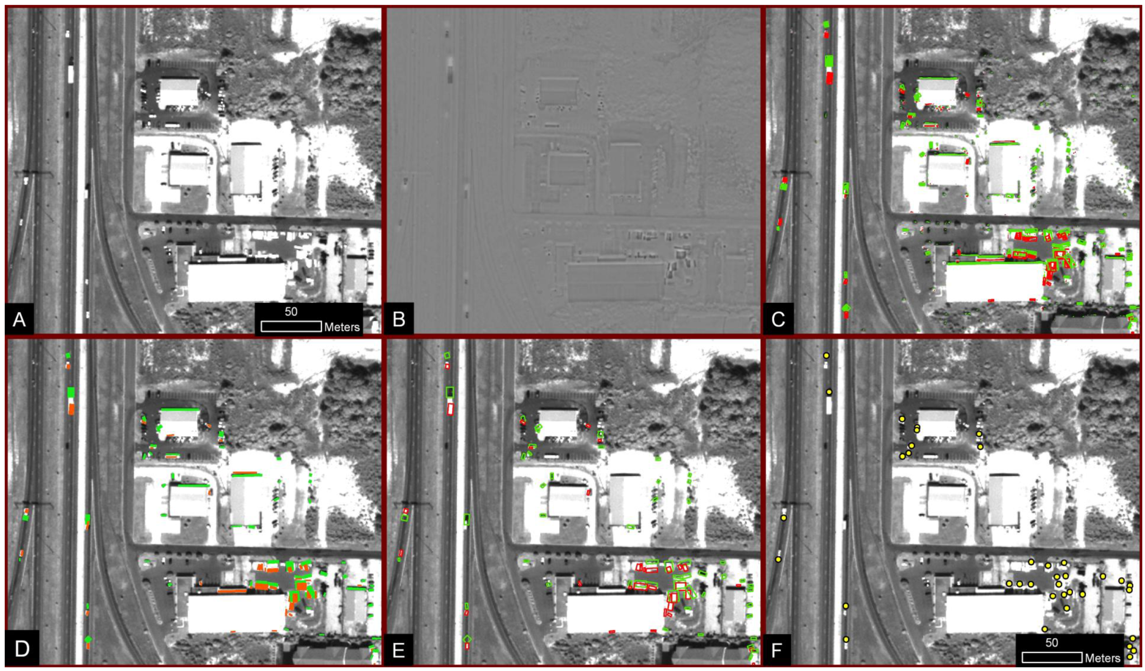
Figure 3 contains a high-speed corridor with a few vehicles on the north-south trending road and includes portions of the industrial and residential sections. Image quality is rated as excellent with zero cloud cover and row/column uncertainties at approximately 45 and 150 meters respectively. This image was collected 25 degrees from nadir and PAN and MS resolutions are 0.72 and 2.88 meters. Global polygons are those returned from the entire 60 km² scene and local polygons are those contained in each subset. Figure 3B shows the cancelation image and Figure 3C the polygons created from the cancelation image. These polygons were then sieved by area (Figure 3D), elongation (Figure 3E) and paired centroids (Figure 3F).

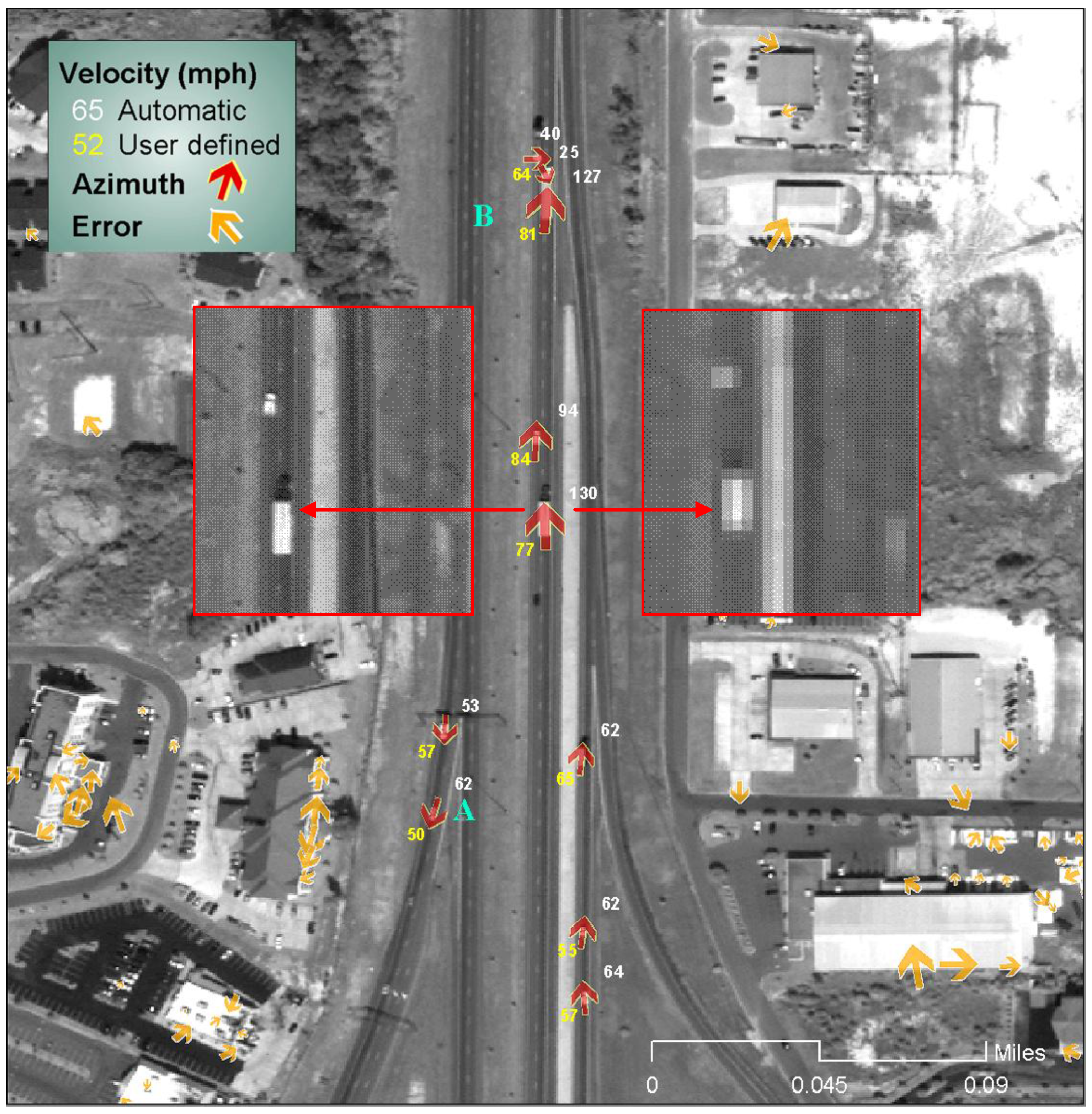
Disproportionate resolution ratios and co-referencing problems create error that is detectable as lineaments around the edges of some polygons. The MS pixels composing of the tractor-trailer in Figure 4 (zoomed area) are larger than those of the PAN and sometimes do not line up properly due to pixel mixing or co-registration. Errors are apparent alongside the highway but most vehicles within the highway boundaries have been given a reasonable speed and bearing. 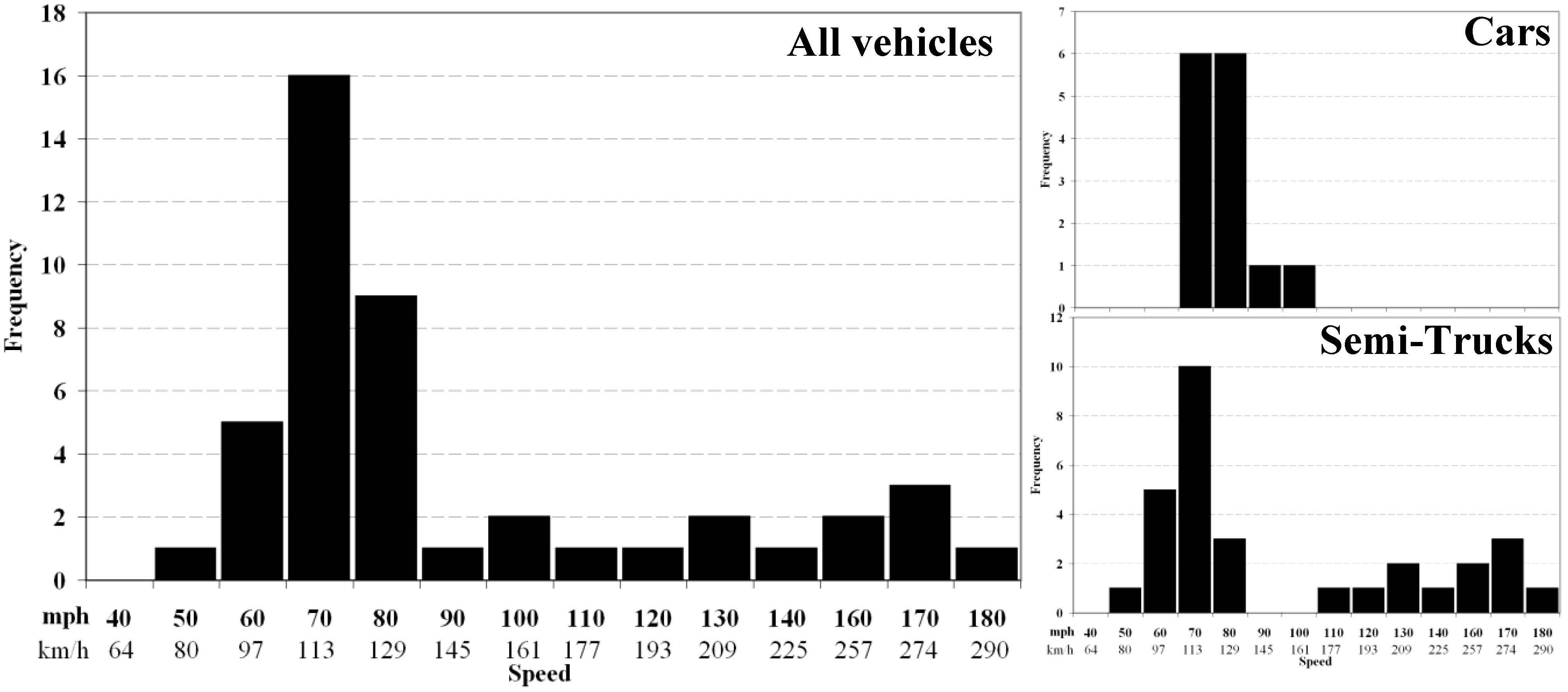Figure 5 shows the distribution of speeds per identified vehicle. When all vehicle types are considered, it can be observed a large spread of speed values. Closer inspection by grouping vehicles into light passenger cars and commercial trucks (Figure 5 smaller histograms), indicates speeds within accepted ranges for light passenger cars and some commercial trucks. Speeds of commercial trucks above 110 mph (177 km/h) are considered incorrect. Slower moving tractor-trailer will return false velocities because the overlap between images. These vehicles are slow and/or large and commonly will not completely escape their original spatial extent before the second image is collected.

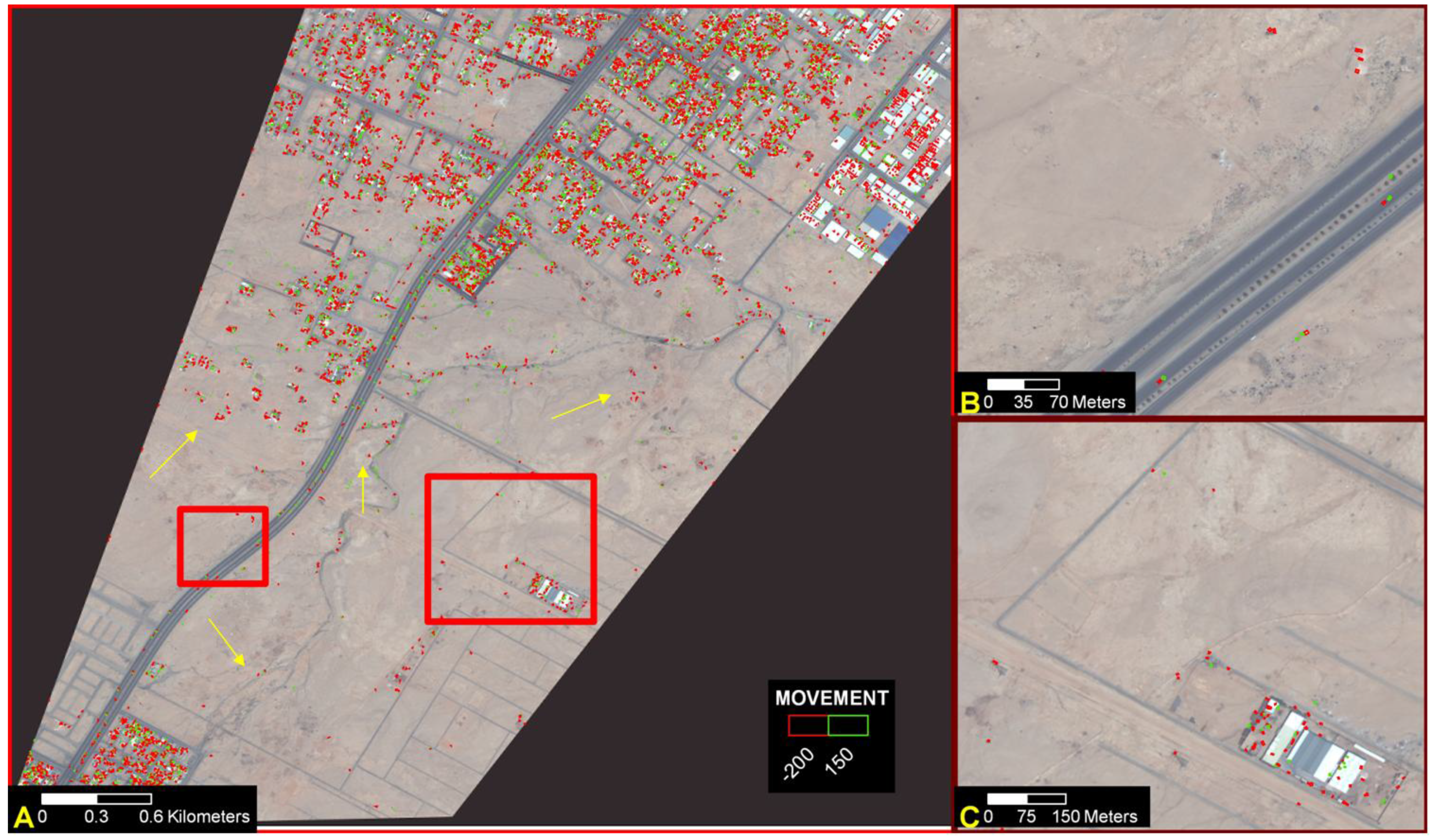
Searching for automobile movement in a desert scene such as Figure 6 is a daunting task, especially if one was to analyze dozens of miles every three days. After applying the MTI to the scene in Figure 6A (Excellent image quality, ~60 m row uncertainty, ~55 m column uncertainty), one can see legitimate targets along the main roads (Figure 6B). Panchromatic GSD for this dataset is 0.63 meters and 2.51 meters for the MS. In this test, thresholds of 150 and −200 returned the best results. As expected, concentrations of false-positives occur near urban areas. DOTs of high contrast with the surroundings are recognized (Figure 6B) and some potential targets were incorrectly highlighted in the barren regions and along structures (Figure 6C). Notice in Figure 6A, yellow arrows showing individual polygons marked in red or green, indicating pixel values below and above the selected thresholds. After the pairing procedure is performed, most are automatically removed, leaving a clean swath of motion free desert.

Figure 3. Panchromatic subset of 60 km² scene 1 (a). Difference method applied (b). Raster to vector conversion (c); 512 local polygons, 284,544 global polygons; sieving the polygons by area (d); 107 local and 34,807 global polygons remain, polygons over 4:1 elongation ratio removed (e); 92 local and 18, 945 polygons remain, and Paired centroids; 38 local and 6,725 global pairs (f).

Figure 3. Panchromatic subset of 60 km² scene 1 (a). Difference method applied (b). Raster to vector conversion (c); 512 local polygons, 284,544 global polygons; sieving the polygons by area (d); 107 local and 34,807 global polygons remain, polygons over 4:1 elongation ratio removed (e); 92 local and 18, 945 polygons remain, and Paired centroids; 38 local and 6,725 global pairs (f).

Figure 4. Study area displaying spatio-temporal attributes of moving targets. Speed annotation in miles per hour. Arrows display direction of target travel; red arrows overlie confirmed moving targets and yellow arrows represent likely error. Zoomed areas illustrate the feature size difference between panchromatic and multi-spectral scenes.

Figure 4. Study area displaying spatio-temporal attributes of moving targets. Speed annotation in miles per hour. Arrows display direction of target travel; red arrows overlie confirmed moving targets and yellow arrows represent likely error. Zoomed areas illustrate the feature size difference between panchromatic and multi-spectral scenes.

Figure 5. Distribution of speed frequency for vehicles on highway segment.

Figure 5. Distribution of speed frequency for vehicles on highway segment.

Figure 6. Desert imagery with 9380 movement polygons (A). Highway with movement pairs and some false-positives alongside (B) and a structure with many incorrect movement polygons with a movement-free perimeter (C).

Figure 6. Desert imagery with 9380 movement polygons (A). Highway with movement pairs and some false-positives alongside (B) and a structure with many incorrect movement polygons with a movement-free perimeter (C).

4.2. Aircraft Detection

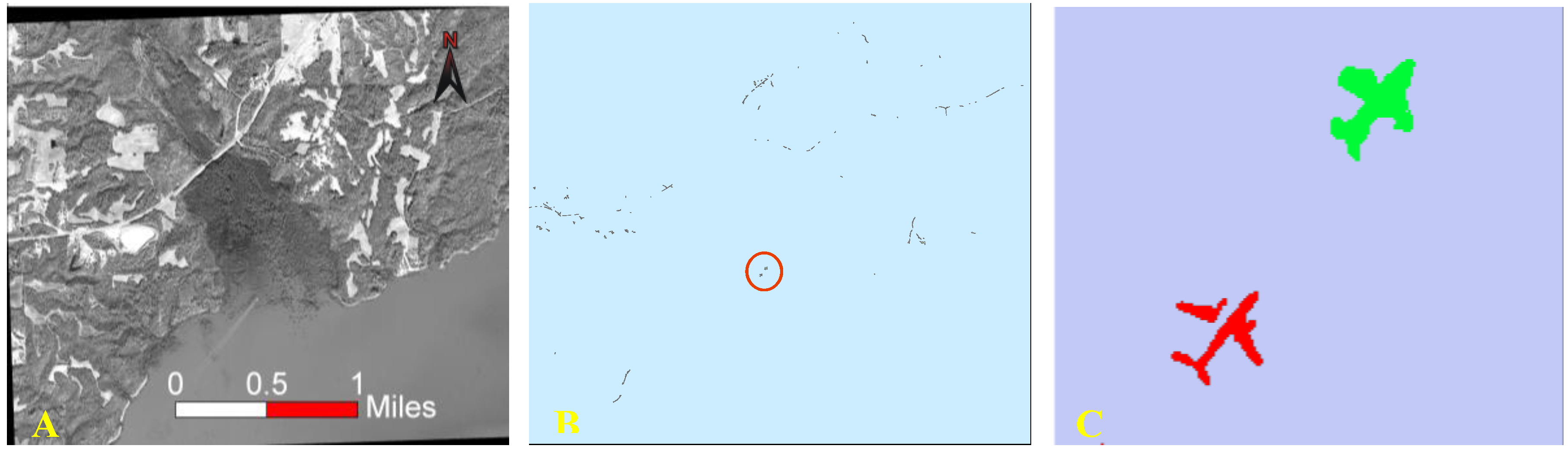
Figure 7 is an example of successful aircraft-at-high-altitude detection using this system. Object A represents a portion of a lake and surrounding countryside. This scene had row/column uncertainties of 90 to 105 meters for both the PAN and MS and excellent image quality. Image differencing and proper thresholds returned 101,377 possible moving targets. Sieving based on min/max areas and elongation reduced this number to 107, allowing for the quick visual detection of this aircraft and an estimate of its speed. Employing common pattern recognition schemes after sieving to scan for aircraft would increase the efficiency and usefulness of the system.

Figure 7. A 16-km² scene of lake and countryside (a). After image differencing and sieving; the red circle contains an aircraft in flight (b), and a zoom of red circle, possible Boeing 737 scenes (c).

Figure 7. A 16-km² scene of lake and countryside (a). After image differencing and sieving; the red circle contains an aircraft in flight (b), and a zoom of red circle, possible Boeing 737 scenes (c).

5. Results and Discussion

5.1. Automobile Detection

This MTI has shown success with detection of small ground targets. Moving targets can be located in satellite optical imagery using this process. Many false-positives were also encountered in this limited testing, mostly products of image properties, spectral inconsistencies, and not co-registering the MS and PAN images. Our system, designed to operate as close as possible as a real-time monitoring tool, relies on the imagery quality provided by the vendors. Some datasets were not suitable in this MTI due to slight spatial shifts from the PAN to the MS. Those images with high row/column uncertainties and low image qualities were more likely in this category. Tests on datasets of GSD pairs 0.6/2.4 meters and 0.7/2.8 meters revealed that elevated GSDs does decrease the effectiveness of the MTI for autos. Sensor movements combined with relief changes are responsible for many false-movement polygons explained later in this section.

In addition to the many false-positives, some vehicles exhibiting low contrast with the environment on the grey scale appeared below the movement threshold. Most cars along roads were flagged but those with similar spectral responses as the surrounding roads sometimes slipped below the threshold. Autos moving cross-country through spectrally complicated terrain will most likely remain undetected, or detectable but difficult to separate from many false-positives. Vehicles below a canopy of even light vegetation are expected to be invisible to this MTI. Although false-positives are abundant near dwellings and sites of high relief, the MTI revealed the movement in homogeneous areas, such as deserted areas.

Masking out areas of severe variation and elevation changes before generating a movement layer will reduce error. Variation in land use tends to result in further pixel mixing and rectification errors. Areas of severe variation and elevation differences, e.g., urban, suburban have many potential false positives and these should be removed from the targeting process. In addition to masking, locations within a scene can be prioritized according to the likelihood of that location containing detectable movement. Vehicle traffic in off-limit areas or other sensitive zones can be targeted in this manner.

Vehicles moving along designated roadways could be further targeted by applying a threshold specific for that area, revealed by examining the digital number differences for autos moving on roadways with similar electromagnetic signatures. For example, detecting a dark car moving along asphalt or a light car moving along concrete requires a threshold level tailored for that zone.

The “movement” of low-relief stationary objects like roadways, and parked autos are most likely a product of co-referencing issues while apparent movement of tall objects is due to parallax. Pixel mixing will also result in apparent stationary movement, sometimes in the form of linear defects. Additionally, as the satellite captures scenes with the PAN and MS sensors, the changes in look angles will be apparent after applying image subtraction as result of parallax. The elongated polygons were cleaned and the smaller ones were recognized as movement.

Some of these problems can be reduced by using high-resolution DEMs. Areas of excessive slope like woodlands and urban zones have a greater likelihood of producing false-positives. Polygons falling entirely in the 0 to 30 degree zones were granted a higher likelihood of being actual movement instead of a false positive from the rapid elevation changes.

5.2. Aircraft Detection

Detecting aircraft movement was a success for those datasets tested. Although noise did exist, the system was able to guide the user’s attention to potential targets. These results suggest that any aircraft over a water body or desert will be detected with low numbers of false positives because of the cancellation of the surrounding homogeneous terrain. Low-altitude aircraft detection is more difficult than locating aircraft at higher altitudes because limitations increase with decreasing detectable surface area. As airplanes are larger and travel faster than automobiles, detection issues from pixel mixing and co-registration are reduced.

5.3. Automobiles Velocity Estimation

The lack of measured information inhibited speed validation. Nineteen semi-trailer trucks and 19 smaller automobiles are detected on the studied portion of the highway (Figure 3) and vehicle speeds are shown in the histogram plot in Figure 5. The semis consistently return unreliable speeds due to overlap but after correcting the centroid placement manually, the speeds returned are reasonable. For this segment, the mean speed of the population is 68.3 ± 3.2 mph with 90% confidence. Although the main objective of this MTI is detect movement in a semi-automated fashion rather than accurately estimate speeds, most of the speeds found for individual smaller automobiles were consistent with the speed limit of the highway investigated and similar results from other investigators such as Xiong [15] and Pesaresi [19].

The mean bearings of the independent north and south bound populations were calculated independently as 3.3 ± 8.5° and 180.3 ± 2.0° respectively with 90% confidence. The bidirectional traffic velocities show that the opposing lanes travel in nearly opposite directions (on average three degrees of perfectly opposing directions). The difference in the variability of the north bound and south bound populations are slight and inexplicable.

5.4. Aircraft Velocity Estimation

The plane detected (Figure 7) is apparently traveling 793 mph, 31 mph in excess of mach 1 at sea level, trending northeast. Speed calculations are unreliable without specific knowledge of the altitude of flight. Representing an airplane in the air on a 2D surface ignores the geometry of a plane in flight in relation to the sensor. Increased altitudes lead to greater unreliability. Although planes are hardly unique, if the model was identified, a relative scale for that altitude using the plane’s dimensions could lead to a better estimate of speed.

6. Conclusions

A simple, semi-automated, and efficient method has been presented for locating vehicles in motion in large QuickBird scenes. It is evident that some airplanes and automobiles in motion are detectable using two optical satellite images differing in both spatial and spectral resolution. Image subtraction, thresholding, and sieving techniques produce polygons which most likely are representative of objects in motion. Proper target recognition is limited by several factors: a target must be in motion at acquisition; a target must be of sufficient contrast from its surrounding environment; and a target must be moving at a detectable speed without overlap onto other targets. While this system detects objects in motion from the imagery, false-positives are also labeled as moving objects. Issues arise from sensor movement during acquisition and images exhibiting reduced quality.

Velocities returned by the MTI will always be suspect, the accuracies depending on the quality of the imagery, centroid determination and pairing, and polygon building. Realistic speeds and bearings are returned using actual pairs of polygons representing the initial and final location of vehicles. This technique will become more valuable with sensors of elevated spatial resolutions. Spatial resolution is a limiting factor for a successful MTI, and is extremely important for auto detection and less so for aerial vehicles. Before using this MTI, an operator must be aware of the limitations of this system. One cannot assume that all moving targets will be flagged or that all flagged objects are moving. If a threshold was chosen to return all movement within a scene, the proportion of false-positives to actual movement would be immense.

After noting the quality of the dataset, the imagery is compared for analysis of the micro-change and the translation of moving autos. With a prior knowledge of the target and search area, a user is able to select a threshold which minimizes noise while pinpointing valid targets. A user can mask out areas showing high variability or relief so that a local threshold may be used for improved results. Ground vehicles must be moving at least 6 mph (9.5 km/h) with perfect co-registration in order to be detected (also shown by [19]). Vehicles must also be of sufficient contrast with their environment to be distinguished from noise returned from subtracting two scenes of different spectral resolutions. A number of false-positives can be flagged as such and removed, but many are classified as movement. Additionally, the effects of relief should also be considered. In this study, the regions investigated are topographically flat therefore minimizing the effect of relief on the movement estimation. The user must exercise judgment on the validity of the movement.

After detection, the movement polygons can be paired to find a vehicle’s speed and bearing. Pairing introduces the possibility of erroneous pairs due to traffic concentrations or the possibility of false movement. Some polygons cannot be appropriately paired because the pixel value differences representing their original or final location passed below the threshold.

This Moving Target Indicator can be used to flag aircraft flying at high altitudes (Figure 7), and judging from the success with small automobiles (Figure 3, Figure 4, and Figure 5), light aircraft at lower altitudes. Aircraft can be flagged in desert terrain and in heavily forested zones with fewer false positives compared to dense, urban scenes.

Detailed traffic studies are not suitable for this MTI. Monitoring zones for movement is the likely interest from commercial and government sectors. Although we recognize the limitations for moving ground target recognition, it is surmised that an MTI incorporating inexpensive, commercial, optical, satellite imagery would supplement current surveillance programs. Inexpensive and readily available, an MTI incorporating satellite imagery is an obvious choice for a surveillance area. The shutter speed of the QB sensor and its poor temporal resolution limits the value of feedback, but an optical-based system involving a cluster of such sensors could reduce the revisit interval weakness. Thus, when counter detection, launching time, or funding is an issue, wide-area surveillance of most vehicles can be achieved with a cluster of satellite-mounted optical sensors, this MTI, and a trained operator.