Evaluating Potential of MODIS-based Indices in Determining “Snow Gone” Stage over Forest-dominant Regions

Abstract

“Snow gone” (SGN) stage is one of the critical variables that describe the start of the official forest fire season in the Canadian Province of Alberta. In this paper, our objective is to evaluate the potential of MODIS-based indices for determining the SGN stage. Those included: (i) enhanced vegetation index (EVI), (ii) normalized difference water index (NDWI) using the shortwave infrared (SWIR) spectral bands centered at 1.64 µm (NDWI_1.64µm) and at 2.13 µm (NDWI_2.13µm), and (iii) normalized difference snow index (NDSI). These were calculated using the 500 m 8-day gridded MODIS-based composites of surface reflectance data (i.e., MOD09A1 v.005) for the period 2006–08. We performed a qualitative evaluation of these indices over two forest fire prone natural subregions in Alberta (i.e., central mixedwood and lower boreal highlands). In the process, we generated and compared the natural subregion-specific lookout tower sites average: (i) temporal trends for each of the indices, and (ii) SGN stage using the ground-based observations available from Alberta Sustainable Resource Development. The EVI-values were found to have large uncertainty at the onset of the spring and unable to predict the SGN stages precisely. In terms of NDSI, it showed earlier prediction capabilities. On the contrary, both of the NDWI’s showed distinct pattern (i.e., reached a minimum value before started to increase again during the spring) in relation to observed SGN stages. Thus further analysis was carried out to determine the best predictor by comparing the NDWI’s predicted SGN stages with the ground-based observations at all of the individual lookout tower sites (approximately 120 in total) across the study area. It revealed that NDWI_2.13µm demonstrated better prediction capabilities (i.e., on an average approximately 90% of the observations fell within ±2 periods or ±16 days of deviation) in comparison to NDWI_1.64µm (i.e., on an average approximately 73% of the observations fell within ±2 periods or ±16 days of deviation).

1. Introduction

An understanding of vegetation spring phenology is very important in assessing various forestry-related activities (e.g., tree growth, carbon sequestration, and forest fire behaviour among others [1,2,3]). In the Canadian Province of Alberta, the Provincial Government has established a network of lookout towers where to date we have approximately 120 lookout tower sites currently in use across the forested-dominant regions of the province since 1920. During the fire season (i.e., April 1st to October 30th), the primary purpose of these lookout towers is the early detection and reporting of the occurrence of wildfire on the landscape. Since the early 1970’s, the lookout tower operators have been the additional responsibility to observe and record the spring phenological events/variables. These phenological variables play an important role in the Canadian Forest Fire Weather System for predicting fire behavior at landscape level [4]. They describe various phenological stages spanning over spring to late fall; and are divided into four categories: snow stages, grass stages, deciduous stages, and coniferous stages [5]. In this study we are interested in understanding the variable “snow gone” (SGN: defined as the date when 25% or less of the area surrounding a tower is covered by snow [5]), which falls under the category of “snow stages”. In practice, the SGN stage is critical for determining the onset of the forest fire season [4]. The lookout tower-based determination of SGN stages has two limitations: (i) it is a subjective approach as it is based on visual observation, and thus the results potentially may vary from person to person; and (ii) it fails to address geographic variability as the lookout tower network provides only point type information over spatial areas of a few hundreds of hectares. One option to address these concerns is to employ remote sensing-based techniques, which have already been proven as an effective method for delineating forestry-related variables at the landscape level [e.g., 6,7]. In the scope of the paper, we intend to explore the potential of remote sensing-based techniques for determining the SGN stage over the forest-dominant regions in the Province of Alberta.

The most commonly used remote sensing-based indices for determining the onset of the growing season are the normalized difference vegetation index [NDVI: a function of red and near infrared (NIR) spectral bands] and enhanced vegetation index (EVI: a function of blue, red, and NIR spectral bands) [8,9,10,11,12,13]. However, the use of NDVI might have larger uncertainty over the forest-dominant regions (where snow accumulation is very common) to determine the onset of the growing season [14,15]. As EVI exhibits similar responses as NDVI at the onset of growing season [13], we could also assume that EVI might respond similar in the presence of snow. However, this requires further investigation.

Another index the normalized difference water index (NDWI: a function of NIR and shortwave infrared (SWIR) [16]) has been implemented successfully in phenological studies [17,18,19,20,21]. In the formulation of NDWI, however, various wavelengths within the SWIR spectral ranges can be employed, e.g., (i) centered at 1.24 µm [16], (ii) centered at 1.64 µm [22,23,24], and (iii) centered at 2.13 µm [25,26,27]. A major challenge remains in the selection of appropriate SWIR spectral band that suits our application of predicting SGN stages. Thus, we intend to use two SWIR bands from MODIS, i.e., band 6 (1.628–1.652 µm) and band 7 (2.105–2.155 µm) in the formulation of NDWI.

The combination of land surface temperature with either vegetation index (e.g., NDVI/EVI [10,12]) or NDWI [18] has been employed to predict various green-up stages. The addition of temperature enhances the overall prediction capacity because temperature has a major influence on plant activities [28]. In general, a daily mean temperature greater than 5 °C is required to trigger the plant’s biological activities [13]. The incorporation of temperature is extremely important when predicting other green-up stages (e.g., grass greening, deciduous leaf out, conifer bud flushing among others [10,12,18]).

Additionally it is also possible to determine the SGN by using normalized difference snow index (NDSI: a function of green and SWIR spectral bands [29]). For example, (i) NDSI in conjunction with surface albedo has been used to quantify SGN [30]; (ii) it was also used to determine the onset of the snow melting time and to characterize the temporal dynamics of NDWI [14]; and (iii) NDSI alone has been used to determine the SGN stages [31]. However, we need to evaluate its performance in our study area.

In this paper, our objectives are to: (i) perform a qualitative evaluation of four MODIS-based indices (i.e., EVI, NDWI_1.64µm, NDWI_2.13µm, and NDSI) in predicting the SGN stages; (ii) compare the SGN values predicted by the efficient indices as determined in objective (i) with the observations available at lookout tower sites across the landscape (as shown in Figure 1 by black hollow circles); and (iii) generate a SGN map using the best predictor as determined in objective (ii) to discuss the spatial variability over the entire Province of Alberta.

2. Methods

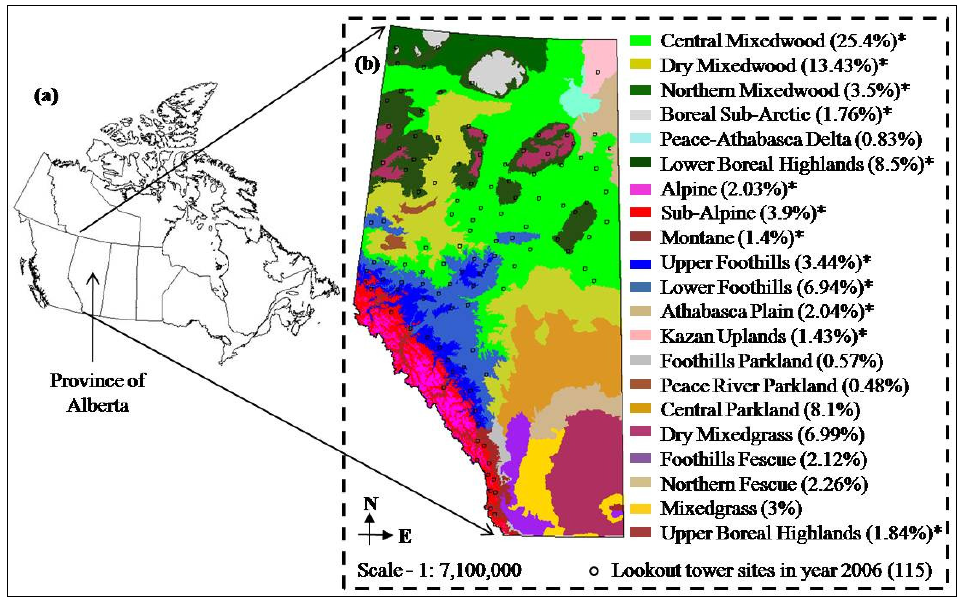
2.1. General Description of the Study Area and Data Requirement

The extent of our study area (i.e., Alberta, Canada) is shown in Figure 1. Geographically, it lies between 49–60°N latitude and 110–120°W longitude. Alberta is characterized as having a continental, relatively humid climate, with cold winters and moderately warm summers. Mean annual temperatures vary between −3.6 °C and 4.4 °C; with summer mean temperatures ranging from 8.7 °C to 18.5 °C, and winter mean temperatures ranging from −25.1 °C to −9.6 °C [32]. The average annual precipitation is between 333 mm and 989 mm [32]. Due to variability in climate, soil type, topography, and vegetation across the province, the study area is divided into 21 natural subregions [32]. These include the 13 mostly forest-dominant natural subregions that occupy about 76% of the total land area in the province where all of the lookout towers are located (see Figure 1 and Table 1 for more details).

Figure 1. (a) Location of the Province of Alberta in Canada; and (b) spatial extent of the 21 natural subregions [32] within the study area with the distributions of “lookout tower sites” (black hollow circles) across the 13 mostly forest-dominant natural subregions (marked as *), where the ground-based observations of “snow gone” were acquired to compare with the MODIS-based indices.

Figure 1. (a) Location of the Province of Alberta in Canada; and (b) spatial extent of the 21 natural subregions [32] within the study area with the distributions of “lookout tower sites” (black hollow circles) across the 13 mostly forest-dominant natural subregions (marked as *), where the ground-based observations of “snow gone” were acquired to compare with the MODIS-based indices.

In this study, we acquired five hundred fifty two scenes of the MODIS-based 8-day composites of surface reflectance data (i.e., MOD09A1 v.005) at a 500 m resolution for the years 2006–2008, which were freely available from NASA. Note that 4 scenes were required to produce the entire extent of the study area, so that eventually we were able to generate one hundred thirty eight 8-day periodical images. For each of the years, there were forty six 8-day periodical images spanning from January 1 to December 31. This data was used to calculate MODIS-based indices (see Section 2.2 for details). In addition, we also acquired ground-based observations of SGN at approximately 120 lookout tower sites across the landscape (see Figure 1 for location information) for the same period. We also required to convert the observed SGN days from day of year [DOY: ranging from 1 to 365(or 366) depending on the leap year] to the no. of periods of the MODIS-based indices for comparison purposes, hence we used the following expression:

$$P=\left(\frac{DOY-1}{8}\right)+1$$

(1)

where, P (=1 to 46) is the no. of periods of the MODIS-based indices; and always takes the previous integer value in event of floating number, e.g., P = 16 if the calculated values of P is in the range of 16.125 to 16.875.

Table 1. Brief description of the 13 mostly forest-dominant natural subregions within Alberta (modified after [32]). Note that the number of lookout towers vary from year to year depending on various factors, e.g., availability of personnel, accessibility, and budget among others.

Natural subregion	Area (Sq. Km.)	Mean annual Temp. (°C)	Mean annual precip. (mm)	Dominant vegetation	No. of lookout towers*
Dry Mixedwood	85,321	1.1	461	Deciduous-dominant mixedwood	2
Central Mixedwood	167,856	0.2	478	Deciduous-dominant mixedwood	24
Lower Boreal Highlands	55,615	−1.0	495	Early to mid-seral pure or mixed forests hybrids	21
Upper Boreal Highlands	11,858	−1.5	535	Conifer dominated	11
Northern Mixedwood	29,513	−2.5	387	Conifer dominated	2
Boreal Subarctic	11,823	−3.6	512	Conifer dominated (Picea mariana )	3
Upper Foothills	21,537	1.3	632	Conifer dominated	15
Lower Foothills	44,899	1.8	588	Conifer-dominant mixedwood	15
Alpine	15,084	−2.4	989	Largely non-vegetated, shrublands	5
Sub-Alpine	25,218	−0.1	755	Mixed Conifer	12
Montane	8,768	2.3	589	Populus, Pinus, Pseudotsuga, grasslands	2
Athabasca Plain	13,525	−1.2	428	Pinus, dunes largely unvegetated	2
Kazan Uplands	9,719	−2.6	380	Mainly rock barrens, pockets of Pinus, Betula, Populus	1

^* N.B. The number of operational lookout towers in 2006.

Table 1. Brief description of the 13 mostly forest-dominant natural subregions within Alberta (modified after [32]). Note that the number of lookout towers vary from year to year depending on various factors, e.g., availability of personnel, accessibility, and budget among others.

Natural subregion	Area (Sq. Km.)	Mean annual Temp. (°C)	Mean annual precip. (mm)	Dominant vegetation	No. of lookout towers*
Dry Mixedwood	85,321	1.1	461	Deciduous-dominant mixedwood	2
Central Mixedwood	167,856	0.2	478	Deciduous-dominant mixedwood	24
Lower Boreal Highlands	55,615	−1.0	495	Early to mid-seral pure or mixed forests hybrids	21
Upper Boreal Highlands	11,858	−1.5	535	Conifer dominated	11
Northern Mixedwood	29,513	−2.5	387	Conifer dominated	2
Boreal Subarctic	11,823	−3.6	512	Conifer dominated (Picea mariana )	3
Upper Foothills	21,537	1.3	632	Conifer dominated	15
Lower Foothills	44,899	1.8	588	Conifer-dominant mixedwood	15
Alpine	15,084	−2.4	989	Largely non-vegetated, shrublands	5
Sub-Alpine	25,218	−0.1	755	Mixed Conifer	12
Montane	8,768	2.3	589	Populus, Pinus, Pseudotsuga, grasslands	2
Athabasca Plain	13,525	−1.2	428	Pinus, dunes largely unvegetated	2
Kazan Uplands	9,719	−2.6	380	Mainly rock barrens, pockets of Pinus, Betula, Populus	1

^* N.B. The number of operational lookout towers in 2006.

2.2. Data Processing

Figure 2 illustrates the steps involved in processing both of the MODIS and ground-based observations. The MODIS-based surface reflectance images were reprojected from their original SIN projection to UTM Zone 12 NAD 83 using MODIS Reprojection Tool [33]. We then mosaicked together four adjacent scenes to create images that covered the entire extent of the study area. At this point, we excluded the cloud contaminated pixels using the “500 m state flags” information (another available layer within the MOD09A1 dataset) from further analysis.

Figure 2. Schematic diagram showing the method followed for analyzing both MODIS-based remote sensing data and the ground-based observations of “snow gone” data.

Figure 2. Schematic diagram showing the method followed for analyzing both MODIS-based remote sensing data and the ground-based observations of “snow gone” data.

The computation of the MODIS-based indices of EVI [34], NDWI_1.64µm [22], NDWI_2.13µm [25] and NDSI [29] were calculated as follows:

$$EVI=2.5\frac{{\rho }_{NIR}-{\rho }_{\mathrm{Re}d}}{{\rho }_{NIR}+6{\rho }_{\mathrm{Re}d}-7.5{\rho }_{Blue}+1},$$

(2)

$$NDW{I}_{1.64 \mu m}=\frac{{\rho }_{NIR}-{\rho }_{SWIR \text{at} 1.64 \mu \text{m}}}{{\rho }_{NIR}+{\rho }_{SWIR \text{at} 1.64 \mu \text{m}}},$$

(3)

$$NDW{I}_{2.13 \mu m}=\frac{{\rho }_{NIR}-{\rho }_{SWIR \text{at} 2.13 \mu \text{m}}}{{\rho }_{NIR}+{\rho }_{SWIR \text{at} 2.13 \mu \text{m}}},$$

(4)

$$NDSI=\frac{{\rho }_{Green}-{\rho }_{SWIR \text{at} 1.64 \mu \text{m}}}{{\rho }_{Green}+{\rho }_{SWIR \text{at} 1.64 \mu \text{m}}},$$

(5)

where, ρ is the surface reflectance for the blue, green, red, NIR, and SWIR spectral bands.

After computing all of the indices, we performed a qualitative evaluation to determine the efficient indices in predicting SGN stages. Here, we considered two of the forest-dominant natural subregions (i.e., central mixedwood and lower boreal highlands, where there were approximately 45 lookout towers; and also these are more vulnerable to forest fire [32]); and executed the following steps:

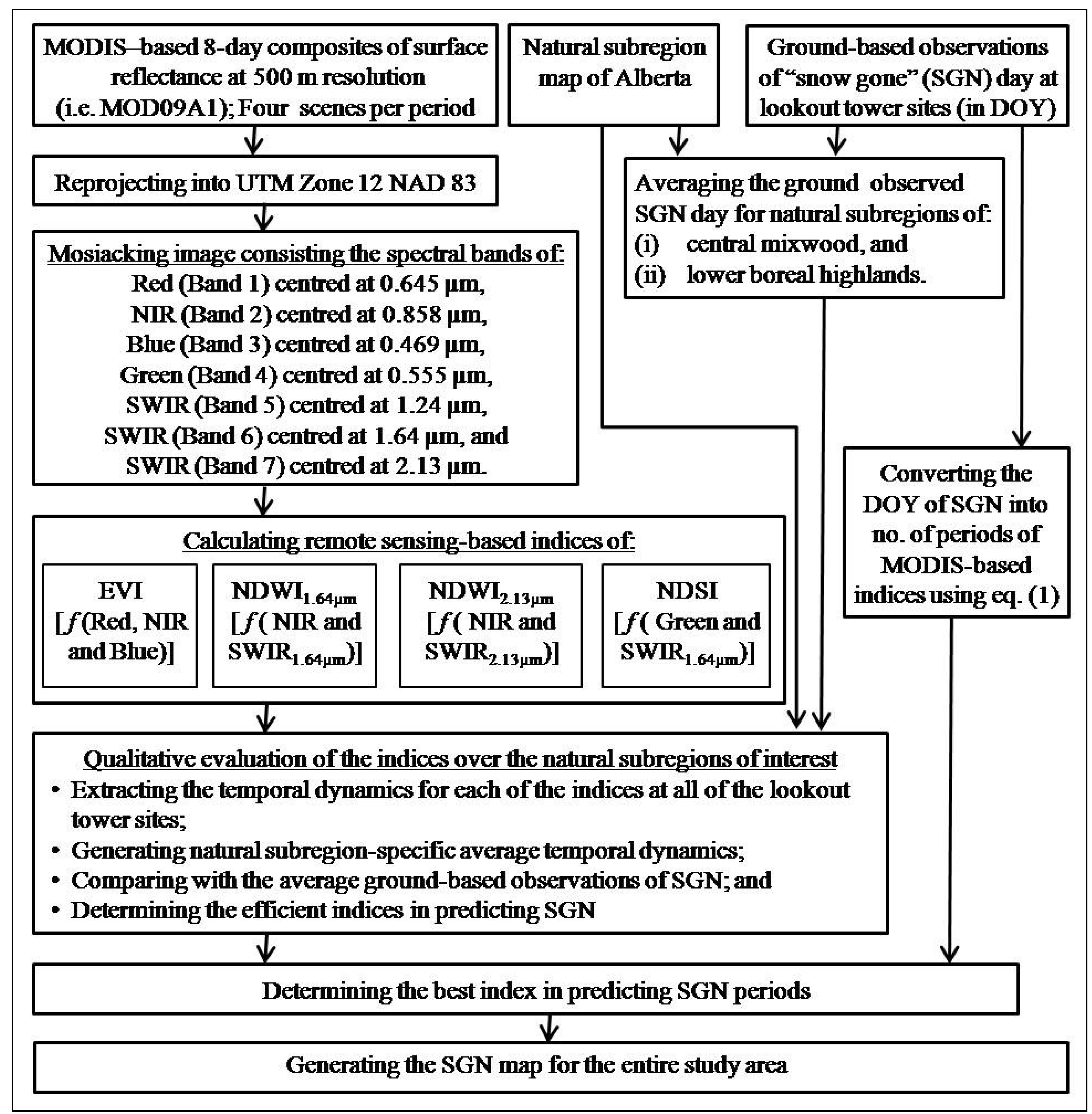
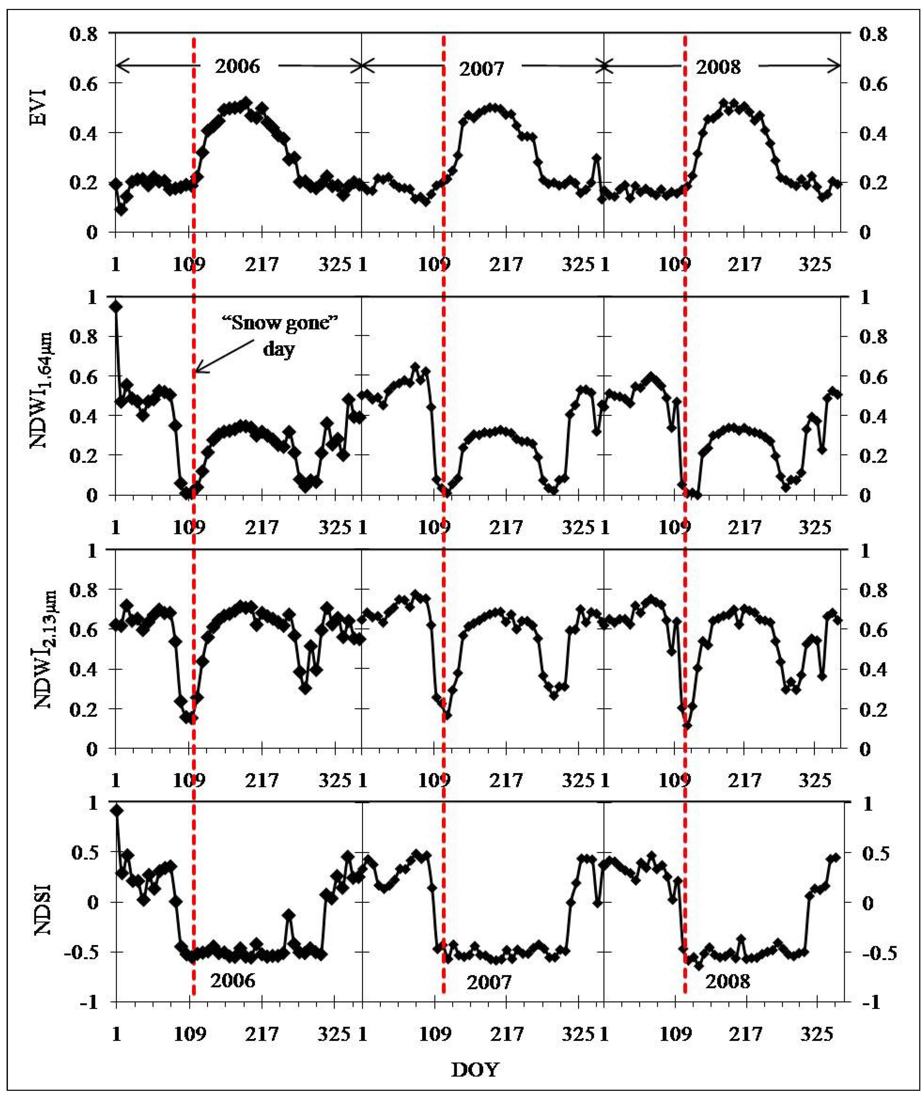
• extracted the temporal dynamics of each of the indices at all of the lookout tower sites; and then generated subregion-specific average temporal dynamics for each of the indices;
• calculated the natural subregion-specific average SGN day using the ground-based observations; and
• compared the values obtained from steps (i) and (iii).

The qualitative evaluation demonstrated that the indices of NDWI_1.64µm, NDWI_2.13µm were better in comparison to others (see Section 3.1. for more details). We observed that the minimum values of these two indices during the spring period (i.e., 65–200 DOY or 06 March–19 July) coincided with the observed SGN stage. Thus, we extracted the temporal dynamics for these two indices at all of the lookout tower sites across the entire study area (see Figure 1 for the lookout tower sites); and declared the minimum values during the spring period as the indices-based SGN period. These were then compared with the ground-based observations of SGN periods. This process led to determine the best predictor index (i.e., NDWI_2.13µm in this study; and see Section 3.2. for more details) in predicting the SGN stages. Finally, we employed the NDWI_2.13µm in generating the SGN maps for the entire study area.

3. Results and Discussion

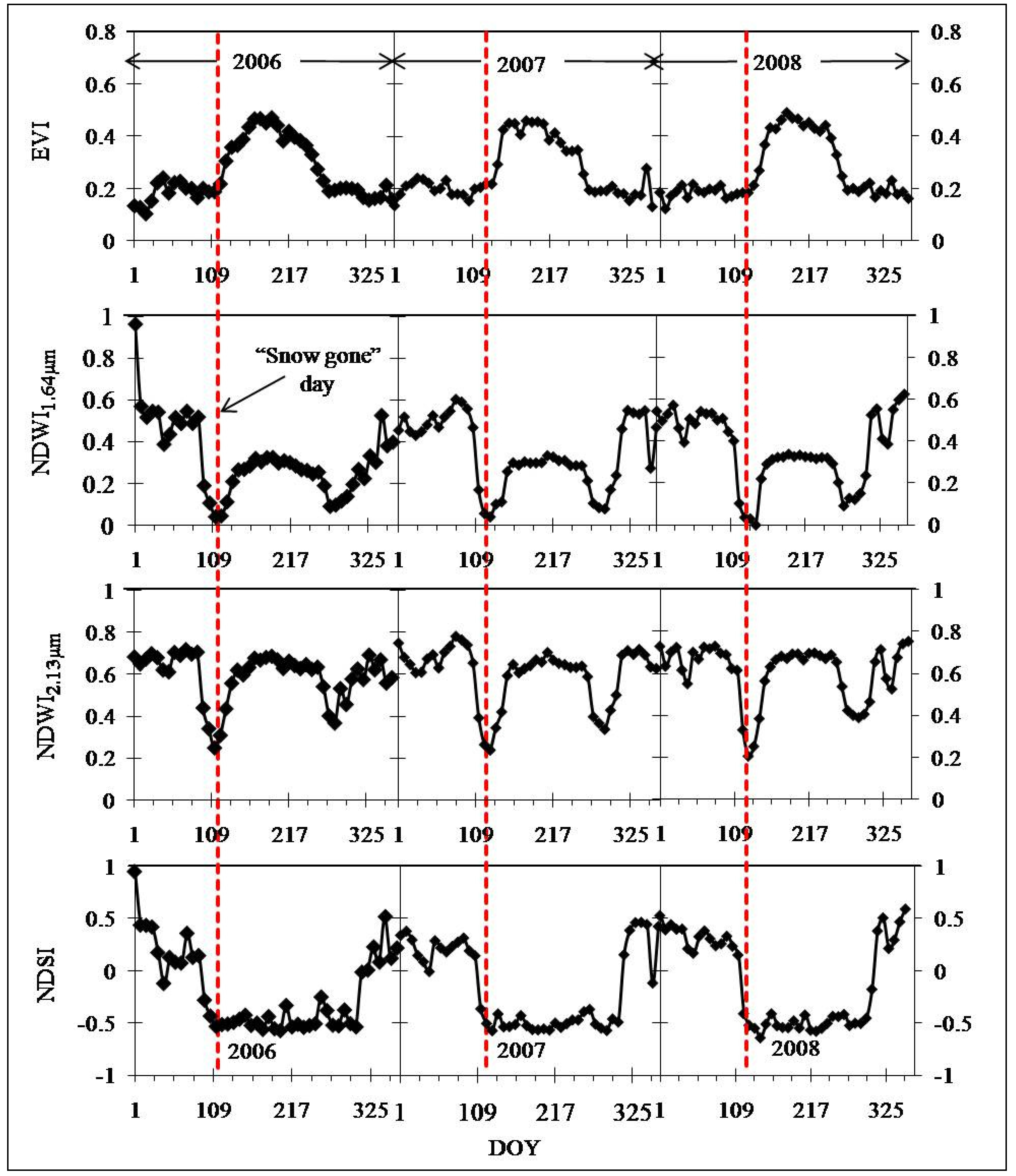
3.1. Qualitative Evaluation of the Remote Sensing-Based Indices in Predicting SGN Stage

Figure 3 and Figure 4 shows the average temporal dynamics for all of the four indices over the natural subregions of central mixedwood and lower boreal highlands for the period 2006–2008. In general, EVI remained low during the winter months (approximately DOY in between 1 and 89) before it started to increase in the spring. These increasing trends might be a result of either snow melting or a combination of both snow melting and greening up [14]. The NDWI’s and NDSI, maintained high values during the winter (DOY in between 1 and 73 on an average) and then started to decrease (about 81 DOY). This might be due to the onset of snow melting [14,15]. The NDWI values were observed to reach a minimum value (about 109 to 135 DOY); and then started to increase again. Similar trends were also observed by others [14,15]. The rises in NDWI might be associated with the SGN stage and/or greening up [14,15]. As the NDWI depicts the snow melting and greening up in opposite directions; the stage corresponds to the minimum values of NDWI might be considered as SGN stage or onset of the growing season as well. In general, a value of 0.4 for the NDSI corresponds to snow disappearance [29], however, this value might even reach to 0.1 depending on the amount and type of vegetation/forests [35]. Additionally, the values of NDSI might reach below “zero” values and refer as “summer conditions” [35]. We also noticed spikes in the temporal dynamics for all of the indices. These might be associated with spatial variation in atmospheric transmissivity and other extrinsic factors that affect the calculations of the MODIS-based indices [7].

Figure 3. Temporal dynamics of averaged values from all of the lookout tower sites for EVI, NDWI_1.64µm, NDWI_2.13µm, and NDSI for the natural subregion of central mixedwood (i.e., which occupies ~25.5% of the province, see Figure 1) for the period of 2006–08. The average SGN day from ground-based observations for the same natural region is shown by the dotted line running vertically.

Figure 3. Temporal dynamics of averaged values from all of the lookout tower sites for EVI, NDWI_1.64µm, NDWI_2.13µm, and NDSI for the natural subregion of central mixedwood (i.e., which occupies ~25.5% of the province, see Figure 1) for the period of 2006–08. The average SGN day from ground-based observations for the same natural region is shown by the dotted line running vertically.

Figure 4. Temporal dynamics of averaged values from all of the lookout tower sites for EVI, NDWI_1.64µm, NDWI_2.13µm, and NDSI for the natural subregion of lower boreal highlands (i.e., which occupies ~8.5% of the province, see Figure 1) for the period of 2006-08. The average SGN day from ground-based observations for the same natural region is shown by the dotted line running vertically.

Figure 4. Temporal dynamics of averaged values from all of the lookout tower sites for EVI, NDWI_1.64µm, NDWI_2.13µm, and NDSI for the natural subregion of lower boreal highlands (i.e., which occupies ~8.5% of the province, see Figure 1) for the period of 2006-08. The average SGN day from ground-based observations for the same natural region is shown by the dotted line running vertically.

Among the four indices, the temporal trends of EVI did not clearly indicate the SGN stage (see Figure 3 and Figure 4 for more details). These results confirmed our assumption that snow might influence the predictive capability of EVI similar to NDVI [14,15]. In terms of NDSI, we observed that the deviation between the ground-based observations of SGN and NDSI-based estimates (when the NDSI-values first went below a threshold of 0.1 during the spring time) were found in the range of −3 to −5 periods (i.e., −24 days to −40 days). The − and + deviations mean the early and delayed predictions respectively in comparison with the ground-based observations for the indices of interest throughout the paper.

Due to the fact that both of the NDWI’s showed a distinct temporal pattern (i.e., the lowest values were found in the early spring as shown as Figure 3 and Figure 4) with the ground-based SGN stages, we considered these two as the efficient indices. Thus we opted to analyse these indices further by assuming that these values were the period of SGN.

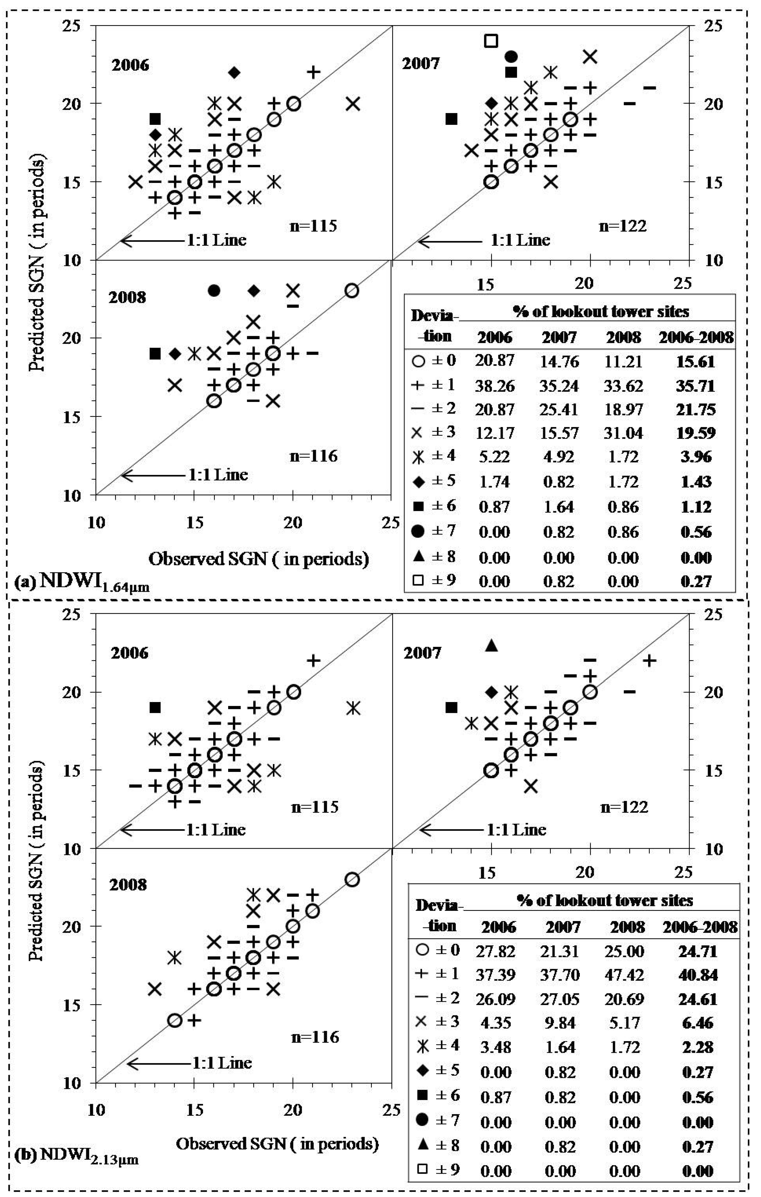
3.2. Determining the Best Index in Predicting SGN Periods

The comparisons between the predicted SGN periods using the efficient indices (i.e., NDWI_1.64µm and NDWI_2.13µm as determined in Section 3.1) and with the ground-based observations at all of the individual lookout tower sites are illustrated in Figure 5. In case of NDWI_1.64µm, on an average approximately 73% of the observations fell within ±2 periods of deviation; 20% in between ±2 and ±3 periods; and the remaining 7% in between ±3 and ±9 periods. In case of NDWI_2.13µm, on the other hand, demonstrated better capabilities in comparison with NDWI_1.64µm. For example, on an average approximately 90% of the observations fell within ±2 periods of deviation; 6% in between ±2 and ±3 periods; and the remaining 4% in between ±3 and ±9 periods. The relatively higher deviations (i.e., > ±4 periods with relatively less probability of ~5% of the time) were, in general, observed in the high elevation area which are located in the natural subregions of alpine, sub-alpine, and upper foothills. The discrepancies between the predicted and ground-based observations of SGN periods might be attributed due to the following factors:

• The ground-based observations were entirely on the basis of visual inspection, thus it highly depended on the experience of an operator to interpret the situation; and
• Spatial resolution of the NDWI’s and ground-based observations might not be in agreement in some instances.

Figure 5. Comparison between the SGN periods at each of the lookout tower sites during 2006-2008 period from ground-based observations and predicted using: (a) NWDI_1.64µm, (b) NWDI_2.13µm. Right and left sides of the 1:1 line represent negative deviation (early prediction) and positive deviation (delayed prediction) respectively. The total no. of operational lookout tower sites for each of the years is denoted by n inside the panels.

Figure 5. Comparison between the SGN periods at each of the lookout tower sites during 2006-2008 period from ground-based observations and predicted using: (a) NWDI_1.64µm, (b) NWDI_2.13µm. Right and left sides of the 1:1 line represent negative deviation (early prediction) and positive deviation (delayed prediction) respectively. The total no. of operational lookout tower sites for each of the years is denoted by n inside the panels.

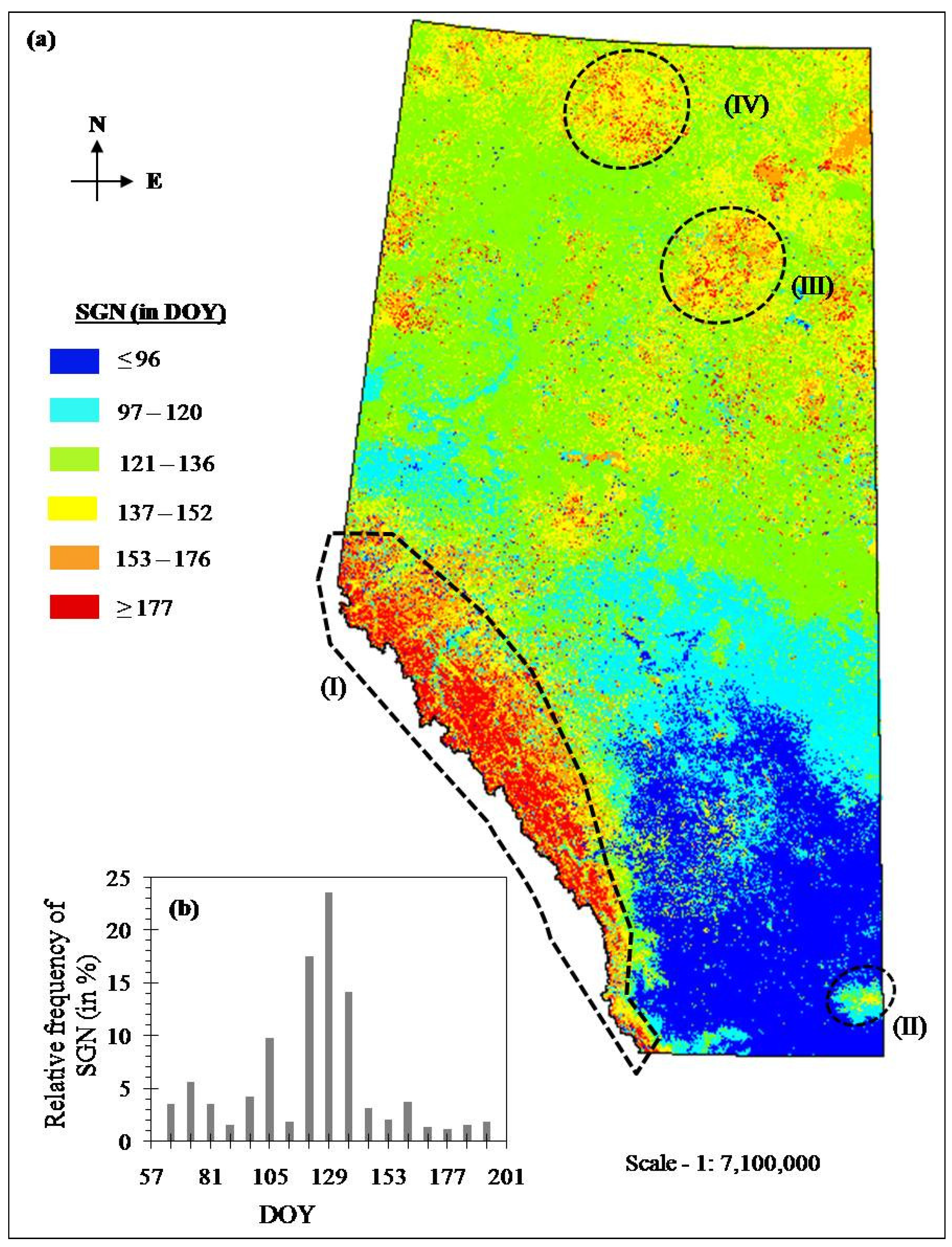
3.3. Spatial Dynamics of the SGN Map

Figure 6 shows an example SGN map generated using NDWI_2.13µm (the best predictor as per Section 3.2) for the year 2008. It revealed that approximately 56% of the times the SGN stages fell in the range of 121–136 DOY. The generalized spatial patterns are discussed as follows:

Figure 6. (a) Spatial dynamics of NWDI_2.13µm predicted SGN map for the entire study; and (b) it’s relative frequency distribution. The polygons I-IV in panel (a) are outlined to have more discussion in the text.

Figure 6. (a) Spatial dynamics of NWDI_2.13µm predicted SGN map for the entire study; and (b) it’s relative frequency distribution. The polygons I-IV in panel (a) are outlined to have more discussion in the text.

• In general, temperature decreases northwards in the northern hemisphere [13], so that the northward increment of SGN stages in our study would be expected.
• The natural subregions in the high elevation areas (i.e., alpine and sub-alpine as shown in polygon I; montane in the middle of polygon II; upper boreal highlands in the middle of polygon III; and sub-alpine in polygon IV) experienced relatively high SGN stages (i.e., in the range of 137–200 DOY). This is reasonable as the high elevation areas experience relatively cooler temperature regime, which influences the snow to stay relatively longer period of time.

4. Concluding Remarks

In this paper we evaluated the potential of four MODIS-based indices (i.e., EVI, NDWI_1.64µm, NDWI_2.13µm, and NDSI) for determining SGN stages in Alberta. A qualitative evaluation over two forest fire prone natural subregions demonstrated that both of the NDWI’s had better capabilities with compare to EVI and NDSI. We then further investigated how both of the NDWI’s could predict the SGN at approximately 120 lookout tower sites across the study area. Our quantitative analysis revealed that the NDWI_2.13µm could better predict the SGN stages in comparison with NDWI_1.64µm. Thus, the MODIS-based NDWI_2.13µm in predicting the variability of SGN stage at landscape level would certainly be useful in the remote areas where the lookout towers are not available. It is a proof of concept in determining SGN stages, so thus, it will potentially be incorporated in the framework of forest fire management in the Province of Alberta. However, we suggest to quantifying the applicability of the described approach before implementing over other biomes/regions in Canada or elsewhere in the world.

References and Notes

1. Linkosalo, T.; Hakkinen, R.; Hanninen, H. Models of the spring phenology of boreal and temperate trees: is there something missing? Tree Physiol. 2006, 26, 1165–1172. [Google Scholar] [CrossRef] [PubMed]
2. Richardson, A.D.; Hollinger, D.Y.; Dail, D.B.; Lee, J.T.; Munger, J.W.; O’Keefe, J. Influence of spring phenology on seasonal and annual carbon balance in two contrasting New England forests. Tree Physiol. 2009, 29, 321–331. [Google Scholar] [CrossRef] [PubMed]
3. Westerling, A.L.; Hidalgo, H.G.; Cayan, D.R.; Swetnam, T.W. Warming and earlier spring increase western U.S. forest wildfire activity. Science 2006, 313, 940–943. [Google Scholar] [CrossRef] [PubMed]
4. Lawson, B.D.; Armitage, O.B. Weather guide for the Canadian Forest Fire Danger Rating System; Northern Forestry Centre, Canadian Forest Service, Natural Resources Canada: Edmonton, Alberta, Canada, 2008; p. 73. Available online: http://fire.ak.blm.gov/content/weather/2008%20CFFDRS%20Weather%20Guide.pdf (accessed on 11 April 2010).
5. Forest Fire Management Terms; Forest Protection Division, Alberta Land and Forest Service: Alberta, Canada, 1999; p. 77. Available online: http://www.srd.alberta.ca/MapsFormsPublications/Publications/documents/ForestFireManagementTerms-AbbrevGlossary-1999.pdf (accessed on 11 April 2010).
6. Hassan, Q.K.; Bourque, C.P.-A.; Meng, F.-R. Estimation of daytime net ecosystem CO2 exchange over balsam fir forests in eastern Canada: Combining averaged tower-based flux measurements with remotely sensed MODIS data. Can. J. Remote Sens. 2006, 32, 405–416. [Google Scholar] [CrossRef]
7. Hassan, Q.K.; Bourque, C.P.-A. Spatial enhancement of MODIS-based images of leaf area index: Application to the boreal forest region of northern Alberta, Canada. Remote Sens. 2010, 2, 278–289. [Google Scholar] [CrossRef]
8. Moulin, S.; Kerogat, L.; Viovy, N.; Dedieu, G. Global-Scale Assessment of vegetation phenology using NOAA/AVHRR satellite measurements. J. Climate. 1997, 10, 1154–1170. [Google Scholar] [CrossRef]
9. Thayn, J.B.; Price, K.P. Julian dates and introduced temporal error in remote sensing vegetation phenology studies. Int. J. Remote Sens. 2008, 29, 6045–6049. [Google Scholar] [CrossRef]
10. Jenkins, J.P.; Braswell, B.H.; Frokling, S.E.; Aber, J.D. Detecting and predicting spatial and inter annual patterns of temperate forest spring time phenology in eastern US. Geophys. Res. Lett. 2002, 29. [Google Scholar] [CrossRef]
11. Ahl, D.E.; Gower, S.T.; Burrows, S.N.; Shabanov, N.V.; Myneni, R.B.; Knyazikhin, Y. Monitoring spring canopy phenology of a deciduous broadleaf forest using MODIS. Remote Sens. Environ. 2006, 101, 88–95. [Google Scholar] [CrossRef]
12. Zhang, X.; Friedl, M.A.; Schaff, C.B.; Strahler, A.H. Climate controls on vegetation phenological patterns in northern mid- and high latitudes inferred from MODIS data. Glob. Change Biol. 2004, 10, 1133–1145. [Google Scholar] [CrossRef]
13. Hassan, Q.K.; Bourque, C.P.-A.; Meng, F.-R.; Richrds, W. Spatial mapping of growing degree days: an application of MODIS-based surface temperature and enhanced vegetation index. J. Appl. Remote Sens. 2007, 1, 013511:1–013511:12. [Google Scholar] [CrossRef]
14. Delbart, N.; Kergoats, L.; Toan, T.L.; Lhermitte, J.; Picard, G. Determination of phenological dates in boreal regions using normalized difference water index. Remote Sens. Environ. 2005, 97, 26–38. [Google Scholar] [CrossRef]
15. Delbart, N.; Toan, T.L.; Kergoats, L.; Fedotava, V. Remote sensing of spring phenology in boreal regions: a free of snow effect method using NOAA-AVHRR and SPOT-VGT data (1982–2004). Remote Sens. Environ. 2006, 101, 52–62. [Google Scholar] [CrossRef]
16. Gao, B.C. NDWI a normalized difference water index for remote sensing of vegetation liquid water from space. Remote Sens. Environ. 1996, 58, 257–266. [Google Scholar] [CrossRef]
17. Xiao, X.; Boles, S.; Liu, J.; Zhuang, D.; Liu, M. Characterization of forest types in north eastern China, using multi-temporal SPOT-4 VEGETATION sensor data. Remote Sens. Environ. 2002, 82, 335–348. [Google Scholar] [CrossRef]
18. Delbart, N.; Picard, G.; Toan, T.L.; Kergoats, L.; Quengan, S.; Woodwand, I.; Dye, D.; Fedotava, V. Spring phenology in Boreal Eurasia over a nearly century time scale. Glob. Change Biol. 2008, 14, 603–614. [Google Scholar] [CrossRef]
19. Picard, G.; Quegan, S.; Delbart, N.; Lomes, M.R.; Toan, T.L.; Woodward, F.I. Bud-burst modelling in Siberia and its impact on quantifying the carbon budget. Glob. Change Biol. 2005, 11, 2164–2176. [Google Scholar] [CrossRef]
20. Jackson, T.J.; Chen, D.; Cosh, M.; Li, F.; Anderson, M.; Walthall, C.; Doriaswamy, P.; Hunt, E.R. Vegetation water content mapping using Landsat data derived normalized difference water index for corn and soybeans. Remote Sens. Environ. 2004, 92, 475–482. [Google Scholar] [CrossRef]
21. Trombetti, M.; Riaño, D.; Rubio, M.A.; Cheng, Y.B.; Ustin, S.L. Multi-temporal vegetation canopy water content retrieval and interpretation using artificial neural networks for the continental USA. Remote Sens. Environ. 2008, 112, 203–215. [Google Scholar] [CrossRef]
22. Wilson, E.H.; Sader, SA. Detection of forest harvest type using multiple dates of Landsat TM imagery. Remote Sens. Environ. 2002, 80, 385–396. [Google Scholar] [CrossRef]
23. Yilmaz, M.T.; Hunt, E.R., Jr.; Jackson, T.J. Remote sensing of vegetation water content from equivalent water thickness using satellite imagery. Remote Sens. Environ. 2008, 112, 2514–2522. [Google Scholar] [CrossRef]
24. Fensholt, R.; Sandholt, I. Derivation of a shortwave infrared water stress index from MODIS near- and shortwave infrared data in a semiarid environment. Remote Sens. Environ. 2003, 87, 111–121. [Google Scholar] [CrossRef]
25. Chen, D.; Huang, J.; Jackson, T.J. Vegetation water content estimation for corn and soybeans using spectral indices derived from MODIS near- and short-wave infrared bands. Remote Sens. Environ. 2005, 98, 225–236. [Google Scholar] [CrossRef]
26. Gu, Y.; Brown, J.F.; Verdin, J.P.; Wardlow, B. A five-year analysis of MODIS NDVI and NDWI for grassland drought assessment over the central Great Plains of the United States. Geophys. Res. Lett. 2007, 34. [Google Scholar] [CrossRef]
27. Yi, Y.; Yang, D.; Huang, J.; Chen, D. Evaluation of MODIS surface reflectance products for wheat leaf area index (LAI) retrieval. ISPRS J. Photogram. Remote Sens. 2008, 63, 661–677. [Google Scholar] [CrossRef]
28. Gyllenstrand, N.; Clapham, D.; Källman, T.; Lagercrantz, U. Norway spruce flowering Locus T Homolog is implicated in control of growth in conifers. Plant Physiol. 2007, 144, 248–257. [Google Scholar] [CrossRef] [PubMed]
29. Hall, D.K.; Riggs, G.A.; Salomonson, V.V.; DiGirolamo, N.E.; Bayr, K.J. MODIS snow-cover products. Remote Sens. Environ. 2002, 83, 181–194. [Google Scholar] [CrossRef]
30. Rinne, J.; Aurela, M.; Manninen, T. A simple method to determine the timing of snow melt by remote sensing with application to the CO2 balances of northern Mire and Heath ecosystems. Remote Sens. 2009, 1, 1097–1107. [Google Scholar] [CrossRef]
31. Dankers, R.; De Jong, S.M. Monitoring snow-cover dynamics in Northern Fennoscandia with SPOT VEGETATION images. Int. J. Remote Sens. 2004, 25, 2933–2944. [Google Scholar] [CrossRef]
32. Natural Regions and Subregions of Alberta; Downing, D.J.; Pettapiece, W.W. (Eds.) Pub. No. T/852; Natural Regions Committee: Government of Alberta, Alberta, Canada, 2006; Available online: http://tpr.alberta.ca/parks/heritageinfocentre/docs/NRSRcomplete%20May_06.pdf (accessed on 11 April 2010).
33. MODIS Reprojection Tool; Version 4.0; USGS: Sioux Falls, SD, USA, February 2008. Available online: https://lpdaac.usgs.gov/lpdaac/tools/modis_reprojection_tool (accessed on 7 September 2009).
34. Huete, A.; Didan, K.; Miura, T.; Rodriguez, E.P.; Gao, X.; Ferreira, L.G. Overview of the radiometric and biophysical performance of the MODIS vegetation indices. Remote Sens. Environ. 2002, 83, 195–213. [Google Scholar] [CrossRef]
35. Klien, A.G.; Hall, D.K.; Riggs, G.A. Improving snow cover mapping in forests through the use of canopy reflectance model. Hydrol. Process. 1998, 12, 1723–1744. [Google Scholar] [CrossRef]