Article

Modeling Methane Emission from Wetlands in North-Eastern New South Wales, Australia Using Landsat ETM+

1
Centre for Geoinformatics Research and Environmental Assessment Technology, School of Environmental Science and Management, Southern Cross University, Lismore 2480, NSW, Australia
2
University of Kurdistan, Erbil, Iraq
3
Marine Ecology Research Centre, School of Environmental Science and Management, Southern Cross University, Lismore 2480, NSW, Australia
*
Author to whom correspondence should be addressed.
Remote Sens. 2010, 2(5), 1378-1399; https://doi.org/10.3390/rs2051378
Submission received: 20 February 2010 / Revised: 10 May 2010 / Accepted: 11 May 2010 / Published: 17 May 2010

Abstract

:
Natural wetlands constitute a major source of methane emission to the atmosphere, accounting for approximately 32 ± 9.4% of the total methane emission. Estimation of methane emission from wetlands at both local and national scale using process-based models would improve our understanding of their contribution to global methane emission. The aim of the study is to estimate the amount of methane emission from the coastal wetlands in north-eastern New South Wales (NSW), Australia, using Landsat ETM+ and to estimate emission with a temperature increase. Supervised wetland classification was performed using the Maximum Likelihood Standard algorithm. The temperature dependent factor was obtained through land surface temperature (LST) estimation algorithms. Measurements of methane fluxes from the wetlands were performed using static chamber techniques and gas chromatography. A process-based methane emission model, which included productivity factor, wetland area, methane flux, precipitation and evaporation ratio, was used to estimate the amount of methane emission from the wetlands. Geographic information system (GIS) provided the framework for analysis. The variability of methane emission from the wetlands was high, with forested wetlands found to produce the highest amount of methane, i.e., 0.0016 ± 0.00009 teragrams (Tg) in the month of June, 2001. This would increase to 0.0022 ± 0.0001 Tg in the month of June with a 1 °C rise in mean annual temperature by the year 2030 in north-eastern NSW, Australia.

1. Introduction

Wetlands are areas of marsh, fen, peatland or water, whether natural or artificial, permanent or temporary, with water that is static or flowing, fresh, brackish or salt, including areas of marine water, the depth of which at low tide does not exceed six meters [1]. Wetlands are important because they are a source of primary productivity; they provide habitats to wildlife; enhance water quality and provide an arena for recreation [2]. There is a need for monitoring wetlands because it allows us to determine whether these ecosystems have changed over time in terms of size, extent and quality. Furthermore, their reliance on rainfall, surface runoff, groundwater levels and evaporation rates make them, and the ecological services they provide, vulnerable to even small climatic changes.
Natural wetlands are a major source of methane (CH4) to the atmosphere, accounting for approximately 32 ± 9.4% to the total methane emission [3,4]. Among the existing greenhouse gases, methane is very important because it contributes approximately 17.7 ± 2.5% to the net greenhouse effect [5,6].
There are different ways to estimate and monitor greenhouse gases such as methane in the atmosphere including experimental and remote sensing approaches. The remote sensing perspective, such as the use of Greenhouse gases Observing Satellite (GOSAT) launched January 23, 2009, produces relatively more accurate estimates of the flux of greenhouse gases on a subcontinental basis. This, therefore, reduces errors by half in identifying the greenhouse gases source and sinks at a subcontinental scale [7]. Furthermore, scaling techniques of greenhouse gases using optical sensing data such as Landsat and Advanced Very High Resolution Radiometer (AVHRR) have been very useful especially for greenhouse gas estimation in regional and global scale. Nevertheless, optical remote sensing data may tend to underestimate emission in tropical environments because of their limitation to cloud cover. Radar systems such as synthetic aperture radar (SAR) sensors on board several satellites (ERS-1, JERS-1, Envisat) have the potential to improve estimates of greenhouse gases across tropical environments because they can penetrate cloud and provide data day and night [8].
There have been some studies related to land-cover analysis/classification using satellite data [9,10,11] and the measurements of methane fluxes from wetlands [12,13]. They identified and classified land cover types such as mangroves, open water, agriculture, forest and urban. Furthermore, they found that accurate and easily reproducible land-cover maps using remote sensing products, which specifically enhance their extent and characteristics, would improve monitoring and land management decisions. Methane fluxes emitted from wetlands were also found to differ significantly between sampling seasons and may increase with climate change by the end of the century [12,13].
Methane production from wetlands is dependent on climatic conditions such as temperature and soil moisture content that affect the metabolic activities of soil microbes. Soil moisture content also affects methane production directly by creating a low redox potential and anaerobic soil environment for methanogens [14,15]. Methane production could also be attributed to substrate availability. High variability in measured methane fluxes from mangroves in Queensland was attributed to dependence on the differences in substrate availability [16].
The quantitative estimation of greenhouse gases such as methane from natural sources using satellite data is very important. This is because natural emissions are closely connected to climate and ecological variables and this interaction constitutes potential feedbacks in the global system. Satellite remote sensing of wetland gaseous emission is very useful especially for large and inaccessible wetland types such as the floodplain wetlands in the Murray-Darling Basin, with a spatial extent of 5,826,600 hectares [17]. This approach has been successfully used to estimate the amount of methane emission from wetlands in Siberia and India [18,19]. These studies estimated methane emission from wetlands such as forested bog, open bog, salt flats, mud flats and swamps. In Australia, especially in the north-eastern part of New South Wales (NSW), there has been no published research of methane estimation from wetlands using satellite data. There are gaps in our understanding as to what the various wetlands contribute to global methane emission at both local and national scale.
The mean annual temperature is projected to increase by 0.2 to 1.6 °C in coastal regions of NSW, Australia by the year 2030 [20]. This would have severe impacts on ecosystem processes such as forests in tropical regions of Australia, which are highly sensitive to climate change within the range that is likely to occur in the next 50–100 years [21].
If temperature is a variable affecting methane production then quantifying the changes expected from a given temperature change can provide important information to the predictive models. This study aims to estimate the amount of methane emission from the coastal wetlands in north-eastern NSW and to estimate the amount of emission with temperature increase using Landsat ETM+.

2. Materials and Methods
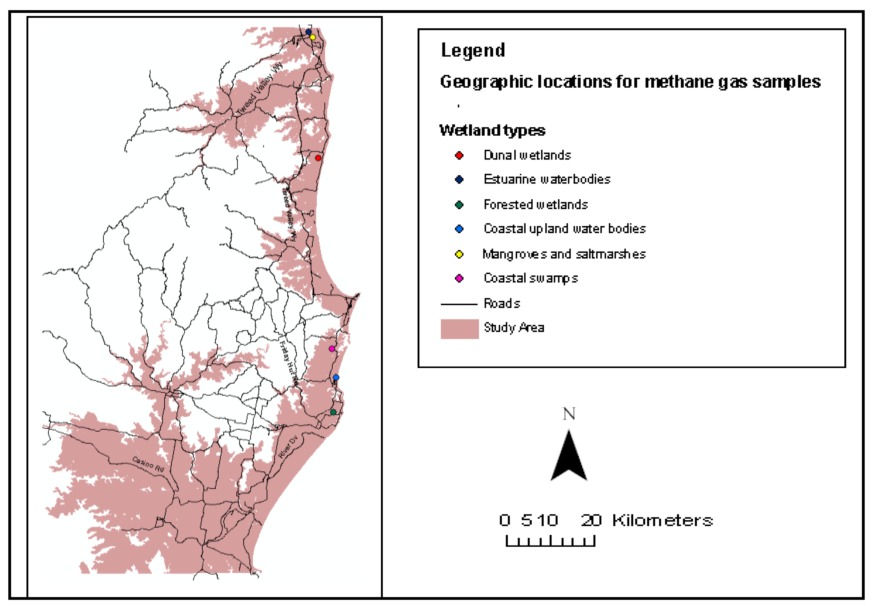
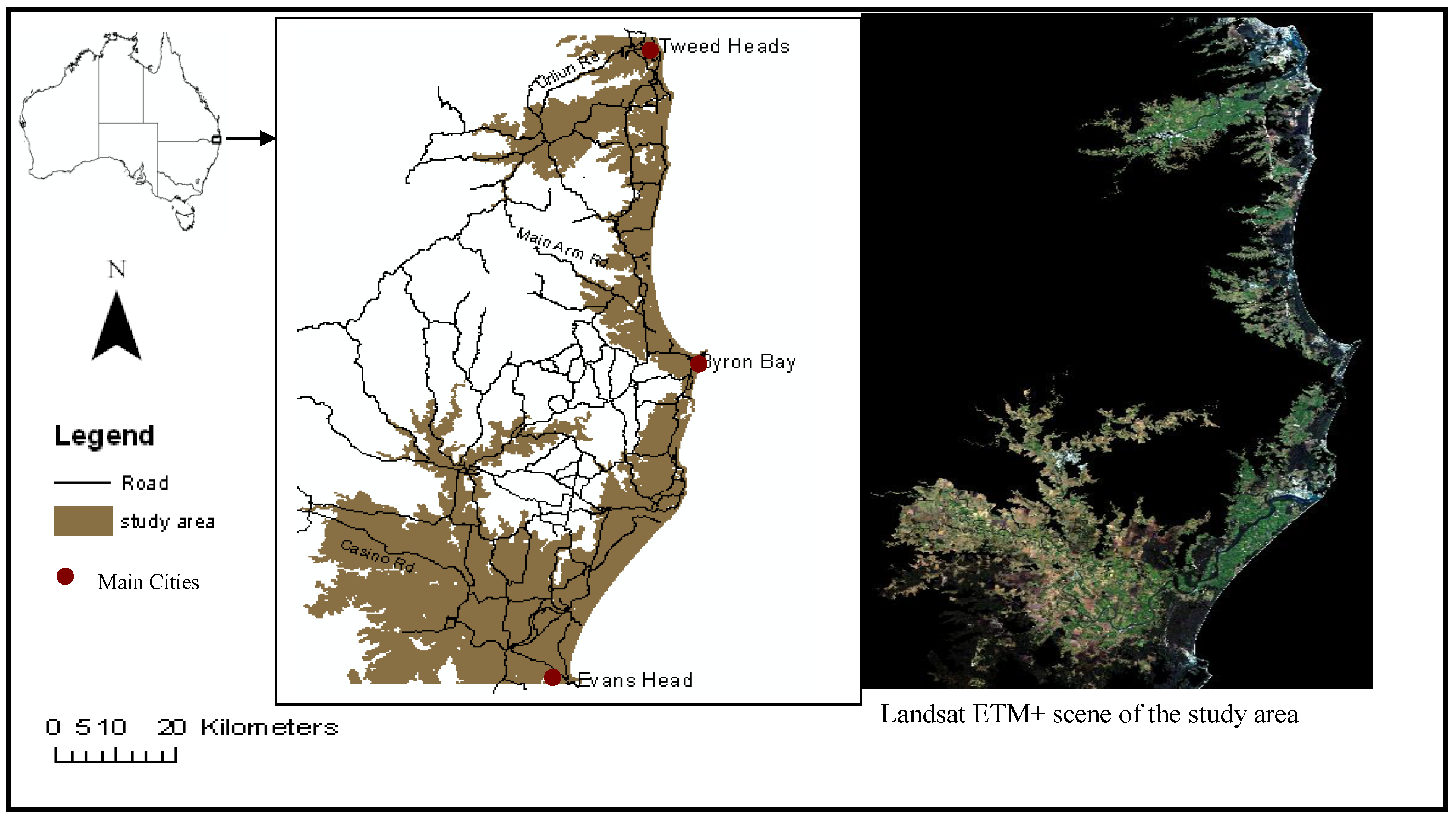
2.1. Study Area

The study area extends from Evans Head to Tweed Heads within 20 m elevation from the coastline of north-eastern NSW (Figure 1). It is a low land area bounded by latitudes 28°09′S and 29°06′S, and longitude 153°00′E Most of the area lies on the Mesozoic sediments of the Clearance-Moreton Basin. It consists of metamorphic rocks and the sediments have been overlain by tertiary volcanics of the Mt. Warning shield volcano. There are outcrops of volcanics in the region consisting of alkaline basalt, andesite and andesitic breccia [22]. Large deposits of Quaternary sand occur along the coast. These consist of marine and Aeolian quartz sands that have formed beaches, dunes and sandsheets. Older Pleistocene dune systems lie inland of the younger Holocene beaches, fore dunes and hind-dunes. The sand masses have been subjected to extensive mining. Estuarine muds and clays occur within creeks and lagoons and peats are present in swamps formed in swales and deflation depressions [22,23,24]. The region is subtropical with mean annual temperature of 20 °C and a mean annual precipitation range of 1,482 mm to 17,560 mm [25].
The wetland types found in this study area include mangroves and saltmarshes, forested wetlands, coastal upland water bodies, dunal wetlands, estuarine water bodies and coastal swamps. Mangroves and salt marshes were estuarine areas, which are subjected to tidal flooding and support mangrove and salt marsh vegetation [26]. Forested wetlands were dominated by trees and occurred on fertile soils, mostly at low altitude. The dominant forested vegetation in the area was broad-leaved paperbark (Melaleuca quinquenervia). Coastal upland water bodies were large or small fresh or brackish water bodies along the coast and included lakes, rivers and ponds. Estuarine water bodies were large open saline or brackish water bodies with a relatively narrow permanent or intermittent connection to the sea. Coastal swamps were fresh water wetlands around the coast that consisted of shallow marshes, wet heaths, and meadows vegetated by sedges and aquatic herbs. Dunal wetlands were fresh water wetlands on coastal sand dunes or plains that support woodland, heathland, sedges, and rushes.
Figure 1. Study Area: north-eastern NSW Australia.
Remotesensing 02 01378 g001

2.2. Satellite Data

The spectral bands used to model methane emission from the wetlands in north-eastern NSW were the optical visible, near-infrared and thermal bands. Visible and Near-Infrared bands were used to extract wetland class information while the thermal band was used to extract land surface temperature, which is an important determinant of methanogenesis. Landsat ETM+ data of June 2001 were used to estimate methane emission from the wetlands. This was due to the availability of cloud free images and also because of its high spatial resolution in the thermal band i.e., 60 × 60 m, compared to Landsat TM with a thermal band of 120 × 120 m. The spectral bands of Landsat ETM+ used (Table 1) were bands 1–4 and band 6.
Table 1. Spectral range and spatial resolution of Landsat ETM + used.
BandsSpectral range (Microns)Spatial resolution
Band 10.45–0.5230 × 30 m
Band 20.52–0.6030 × 30 m
Band 30.63–0.6930 × 30 m
Band 40.76–0.9030 × 30 m
Band 610.40–12.5060 × 60 m
The methodology (Figure 2) involved the use Landsat ETM+ satellite data to classify the wetlands and to generate Normalized Difference Vegetation Index (NDVI) for the wetland classes. The NDVI of the vegetation was used to estimate emissivity for the wetland classes. The emissivity of the wetland classes was needed in order to correct the spectral emissivity of the blackbody temperature generated. This is because NDVI values of vegetation have been found to be strongly correlated with thermal emissivity [27]. Pre-processing (e.g., geometric and radiometric corrections) and supervised classification of the Landsat ETM+ data were performed and the wetland classes exported to geographic information system (GIS) for further analysis of area covered by each class. Accuracy assessment of the classified wetland map was carried out using orthophoto, Google Earth and groundtruthing. The classified wetland map was further reclassified using the spatial analyst tool in ArcGIS in order to assign the mean emissivity values for each wetland type which was further used to correct the spectral emissivity of the blackbody temperature generated.
Figure 2. Schematic representation of methodology.
Remotesensing 02 01378 g002
Band 6 was pre-processed and used to generate land surface temperature (LST) for the wetland classes. Climate data from the Bureau of Meteorology was used to validate the generated LST and to obtain precipitation and evaporation information for the study area. Observed methane fluxes for the wetland classes were obtained by field and lab experiments. The productivity factor of methane emission from the wetland classes were estimated using net primary productivity values from literature. The area of the wetland classes, observed methane flux, productivity factor, T-factor, precipitation and evaporation ratio were used to model methane emission estimates from wetlands in north-eastern NSW Australia.

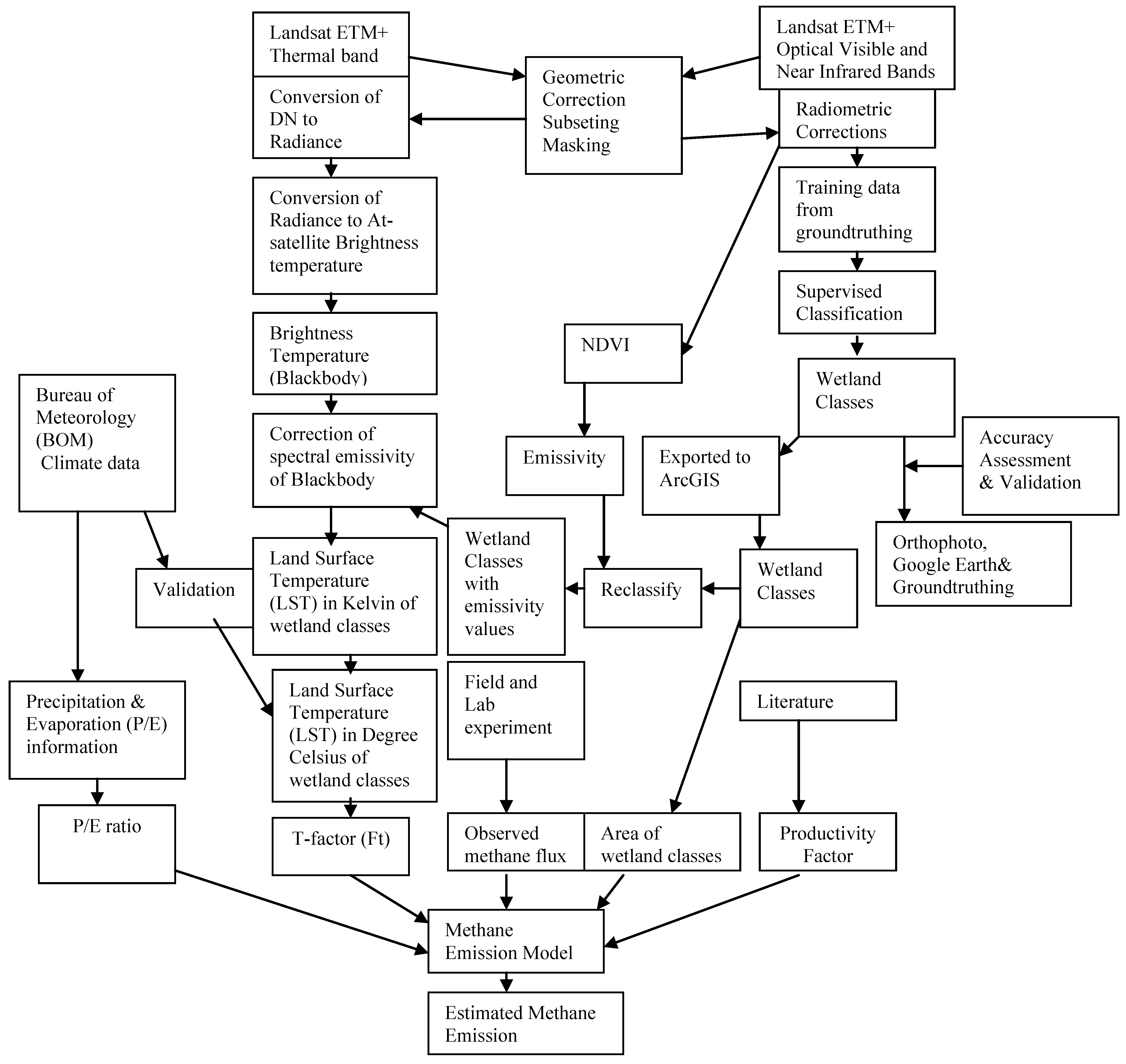
2.3. Methane Emission Estimation

Methane production process from the wetland soil is dependent on soil moisture, wetland extent, vegetation type, water table depth and temperature [28]. Higher temperatures alone would increase methane production in saturated areas, but would also cause these saturated areas to shrink resulting in a net methane reduction, while higher precipitation alone would raise the soil moisture, water table, and expand the wetland extent thereby resulting in a net increase in methane. However, an exception to these relationships is for small increase in temperature (1 °C) and precipitation (5%), for which the temperature increase can cause a slight increase in methane emission [13]. Furthermore, the vegetation type in an ecosystem would influence the net primary productivity (NPP) of the ecosystem and this is proportional to methane production [29]. The estimation of methane production from the soil in this study assumes the methane emission processes depend linearly on temperature.
This was carried out using equation 1 modified from Agarwal and Garg [18] and Liu [14].
ECH4 = Eobs. Ft. A. P. fw
where:
  • ECH4 = Estimated Methane Emission
  • A = Area of wetland classes
  • Ft = T factor
  • Eobs = observed methane flux from different wetland classes,
  • P = Productivity factor
  • fw = P/E = Precipitation /Evaporation ratio, Where: fw {P/E if P ≤ E} or {1 if P > E}.

2.3.1. Estimating Area of Methane Emitting Wetlands

The area of methane emitting wetlands was estimated from classified wetland map produced using Landsat ETM+ data. This was carried out using the following image processing steps: (a) Georeferencing (b) Subseting (c) Masking (d) Converting DN to Radiance (e) Converting Radiance to Reflectance (f) Supervised Classification and (g) Accuracy Assessment
The Landsat ETM+ satellite images (five scenes) acquired on June 21st 2001 were converted from Binary BIL format into ER Mapper data format in ER Mapper software version 7.1. The Landsat scenes were georeferenced based on an orthophoto and re-projected into the UTM-WGS 84 projection. Twenty-four ground control points were used in the rectification process with an overall RMS error of less than 1 pixel. The images were later subsetted to the study area and a digital elevation model (DEM) was used to mask out all areas that are more than 20 m altitude from the coastline. This is because the coastal zone was defined as all areas less than 20 m elevation from the coastline.
Radiometric correction was carried out in the visible and near infrared regions of the satellite images. Radiometric correction entails the correction of image pixel values for sun elevation angle variation and the calibration of images to account for degradation of the sensors over time. The changes in sensors calibration factors will obscure real changes on the ground [30]. This process involves the conversion of digital numbers to at-satellite radiances and at-satellite radiance to at-surface reflectance. This radiometric correction process includes atmospheric and illumination corrections.

2.3.1.1. Conversion of DN to Radiance-Landsat ETM+

This was carried out using Equation 2:
Lrad = Bias + (Gain × DN)
where:
  • Lrad = Spectral radiance, W/m2/sr/µm
  • DN = Digital number.
The spectral values of gain and bias for Landsat ETM+ data (Table 2) were obtained from the image header file.
Table 2. Spectral values of bias and gain from the Landsat ETM+ image header file.
BandsGainBias
10.7756863−6.1999969
20.7956862−6.3999939
30.6192157−5.0000000
40.6372549−5.1000061

2.3.1.2. Conversion of Radiance to Reflectance—Landsat ETM+

This was performed using Equation 3:
RTOA = (π × Lrad × d2)/ (ESUNi × cos (z))
where:
  • RTOA: the planetary reflectance
  • Lrad: is the spectral radiance at the sensor’s aperture;
  • π: ≈ 3.14159
  • ESUNi: the mean solar exoatmospheric irradiance of each band
  • d: the earth-sun distance, in astronomical units, which is calculated using the following EXCEL equation [31,32]
  • d = (1 − 0.01672 × COS (RADIANS (0.9856 × (Julian_Day − 4)))).
  • z: solar zenith angle (zenith angle = 90 − solar elevation angle), solar elevation angle is within the header file of the satellite images.

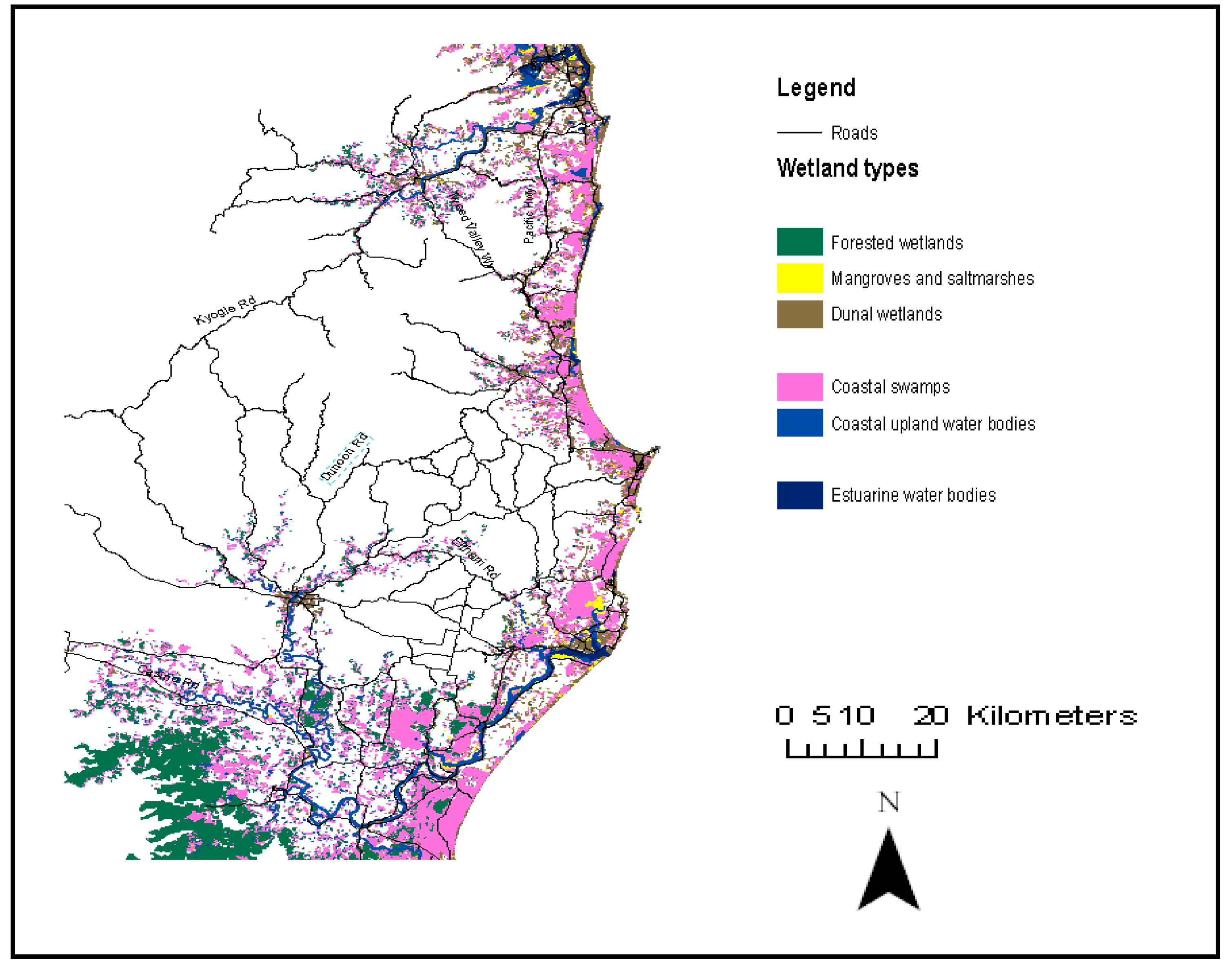
2.3.1.3. Classification

Supervised classification was carried on the Landsat ETM+ image in ER Mapper version 7.1. This was performed on the reflectance images using a set of user-defined classes. This requires digitizing training sites into user-defined polygons based on knowledge of the wetlands classes obtained from regular field visits. Statistics of the training sites were generated and evaluated. The supervised classification was performed using the Maximum Likelihood Standard algorithm. This is because it considers both the means and the variances of the training data in order to approximate the probability that a given pixel belongs to a particular class. Furthermore, it produces better results compared to minimum distance to means or parallelpiped classifiers [33]. Non-wetland areas such as urban and agricultural areas were masked out from the classification.
Accuracy assessment of the wetland classification was performed by comparing the classified map with scenes from Google Earth, color orthophoto and groundtruthing of the region. 312 samples were selected from the classified map through random sampling method from the wetland classes and compared with the referenced maps. Furthermore, groundtruthing was carried out in order to validate the wetland classes. It was performed by randomly selecting the samples in the field and using of a global positioning system (GPS) as a guide to identify the wetland classes. A k × k confusion matrix (error matrix) table was developed and the producer accuracy, user accuracy, overall accuracy and kappa analysis were calculated.
The producer’s accuracy of the wetland classification was performed by dividing the total correct sample units of each wetland category by the total number of the wetland class sample units as indicated by the reference data (i.e., column total). The user’s accuracy was also performed by dividing the total number of correct pixels in each wetland category by the total number of pixels classified in that category (i.e., row total). The overall accuracy of the classification (87.50%) was computed by using the sum of the major diagonal (i.e., the correctly classified sample units) divided by the total number of sample units in the entire error matrix [34]. The kappa statistical value (85.00%) for the classification is a measure of how well the remotely sensed classification agrees with the reference data. The kappa analysis from the classification showed a high correlation between the wetland classification and the reference data used.
The classified wetland map was exported to ArcGIS and their respective areas generated. The following methane emitting wetland types were identified: mangroves and saltmarshes, forested wetlands, dunal wetlands, estuarine water bodies, coastal upland water bodies and coastal swamps.
Normalize Difference Vegetation Index (NDVI) of the reflectance image was also generated. The NDVI was generated for use in the estimation of thermal emissivity of the wetland classification. This was carried out using Equation 4 [35].
NDVI = (Near-infrared − Visible red) / (Near-infrared + Visible red)
The NDVI values were obtained for the following wetland classes: mangroves and saltmarshes, forested wetlands, dunal wetlands and coastal swamps with overlapping NDVI values between classes. The observed mean NDVI values and standard error (SE) were 0.665 ± 0.044 for mangroves and saltmarshes, 0.685 ± 0.054 for forested wetlands, 0.669 ± 0.067 for dunal wetlands, and 0.565 ± 0.095 for coastal swamps.

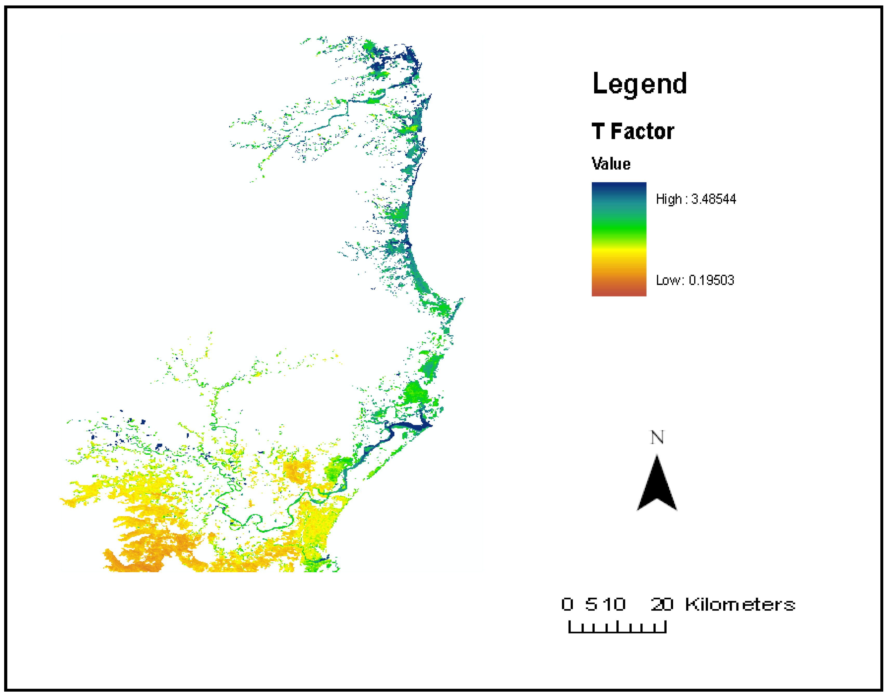
2.3.2. Estimating T factor

The T factor was derived from Equation 5 [14].
F t = F ( T s ) F ( T s ) ¯
where:
  • Ft = T factor
    F ( T s ) = e 0.334 ( Ts 23 ) 1 + e 0.334 ( Ts 23 )
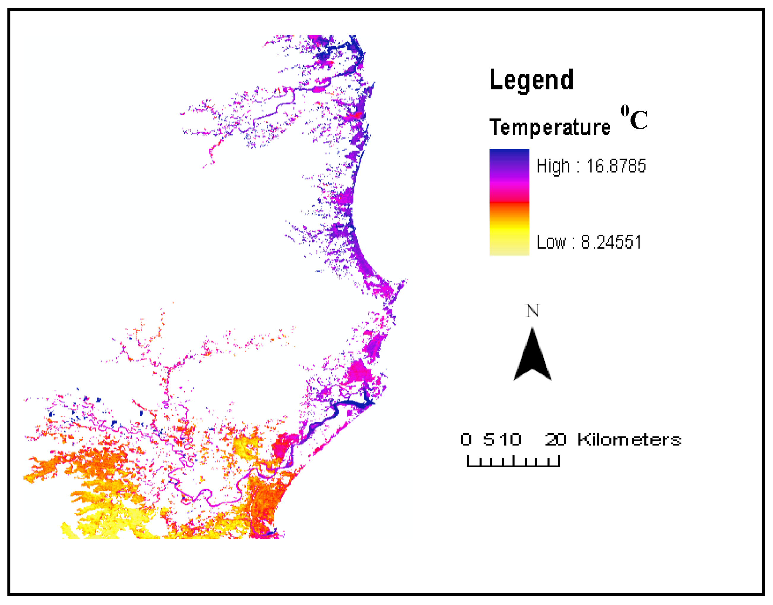
  • Ts = Land surface temperature in Degrees Celsius
  • F ( T s ) ¯ = Mean of F (Ts) over wetlands. It was derived from the F (Ts) image. The F (Ts) image was converted from raster to vector format in ArcGIS and their mean values estimated.
The mean F (Ts) value over the wetlands and standard error was 0.04 ± 0.01.

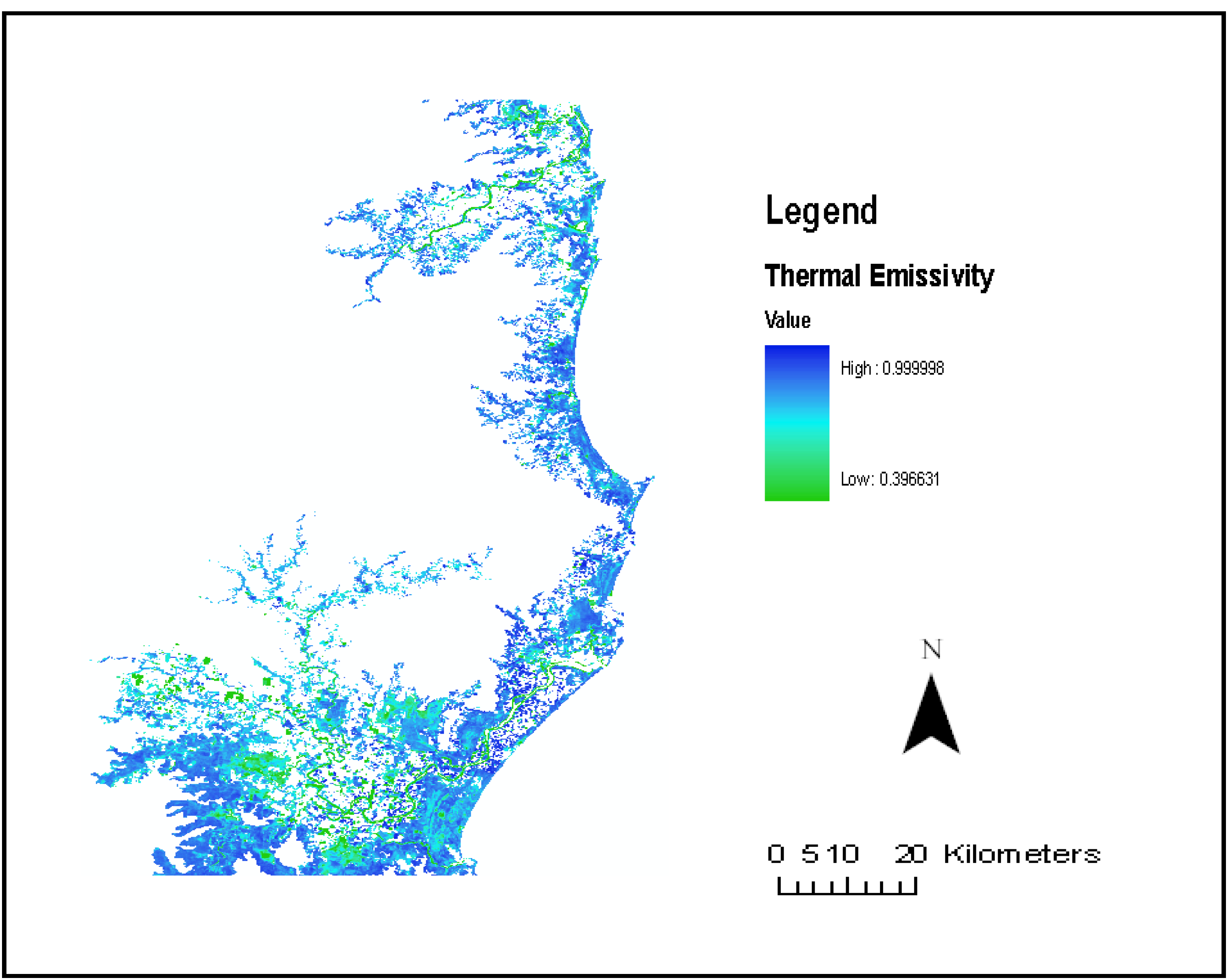
2.3.2.1. Estimating Land surface Temperature (Ts)

In this study, land surface temperature (LST) is an important input factor in the methane modeling process. It was derived from Landsat ETM+ using the thermal infrared band (10.40–12.50 µm), with a spatial resolution of 60 m. The satellite images were georeferenced using an othophoto and re-projected into the UTM-WGS 84 projection. The images were later subsetted to the study area and a DEM was used to mask out all areas that are more than 20 m altitude from the coastline. The following processing steps were further carried out on the Landsat ETM+ band 6 satellite data:

Conversion of Digital Number (DN) to Spectral Radiance

The DN of the thermal infrared band (band 6) was converted to Radiance using Equation 7 [36].
L λ = 0.0370588 × DN + 3.2
where:
  • L λ = radiance, W/m2/sr/µm
  • DN = digital number

Conversion of Spectral Radiance to At-Satellite Brightness Temperature (Blackbody temperature)

The spectral radiance was converted to at-satellite brightness temperature using equation 8, assuming uniform emissivity [36].
T B = K 2 ln ( K 2 L λ + 1 )
where:
  • TB = at-satellite temperature in Kelvin
  • L λ = spectral radiance W/m2/sr/µm
  • K2 and K1 are pre-launch calibration constants. For Landsat-7 ETM+
  • K2 = 1,282.71 K
  • K1 = 666.09 mW cm−2 sr−1 μm−1.
However, the temperature obtained (TB) is with reference to a black body (perfect absorber and emitter of radiation) assuming a uniform emissivity. There is therefore a need to correct the spectral emissivity with respect to the land cover. Emissivity is the ratio between emittance from an object in relation to emittance from a blackbody at the same temperature [35].The spectral emissivity for the various wetland types were derived using their NDVI values [27]. According to Van de Griend and Owe [27], when the NDVI value of natural land surface is between 0.157 and ~0.727, then emissivity may be acquired approximately from NDVI index of the vegetation using Equation 9 [27].
ε = 1.0094 + 0.047 ln (NDVI)
where:
  • ε = emissivity
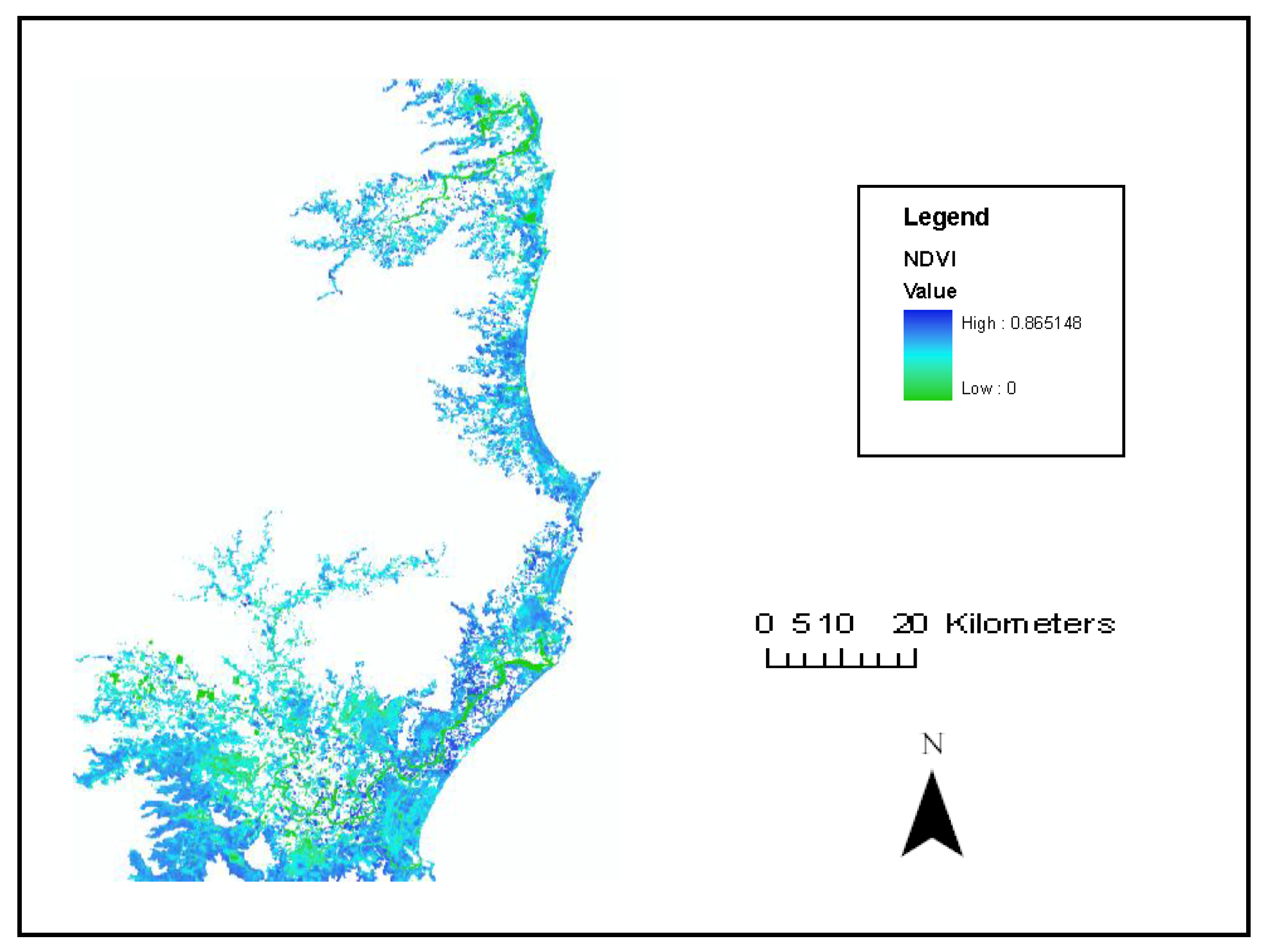
  • NDVI = Normalized Difference Vegetation Index.
A constant emissivity value of 0.986 for water (estuarine water bodies and coastal upland water bodies) was adopted from the emissivity classification scheme by Snyder et al. [37].
The observed mean emissivity values for the wetland classes were as follows: mangroves and saltmarshes = 0.990 ± 0.004, dunal wetlands = 0.991 ± 0.007, forested wetlands = 0.992 ± 0.004, coastal swamps = 0.983 ± 0.009. This is, however, limited to wetland vegetation and would not be applicable to bare soil and water with NDVI values of less than 0.157. Furthermore, a change in the quality of the wetland vegetation would also change the thermal emissivity values of the wetland.
The wetland map was reclassified using these values and was used to correct the spectral emissivity of the blackbody temperatures (TB).
The emissivity corrected land surface temperatures (St) were then computed using Equation 10 [38].
S t = T B 1 + ( λ × T B / ρ ) ln ε
where:
  • St = emissivity corrected land surface temperatures (LST) in Kelvin
  • λ = wavelength of emitted radiance,
  • ρ = h × c/σ (1.438769 × 10⁻² m K, second radiation constant), σ = Boltzmann constant (1.3806503 × 10⁻²³ J/K), h = Planck’s constant (6.626068 × 10⁻³⁴ J s), c = velocity of light (2.99792 × 10⁸ m/s).
  • TB = at-satellite temperature in Kelvin
  • ε = emissivity of wetland classes
The unit (Kelvin) of the emissivity corrected LST was converted to degree Celsius using Equation 11.
I1 − 273.15
where: I1 = St.
Land surface temperature values (Table 3) were then estimated for the different wetland classes. These values were validated from climate data obtained from the Bureau of Meteorology. Furthermore, according to the IPCC [4] report, the mean annual temperature will rise by 0.2 to 1.6 °C by the year 2030. This study assumes a 1 °C rise in mean annual temperature by the year 2030 and this value was added to the LST generated. The following estimated T factor values (Table 4) for the different wetland classes were then generated based on the estimated land surface temperatures. Furthermore, a projected T factor assuming a 1 °C rise in mean annual temperature by the year 2030 was also generated using the projected LST. This was further used to predict methane emission estimates with 1 °C rise in mean annual temperature assuming every other variable is kept constant.
Table 3. Estimated mean LST and projected LST for the wetland classes in the winter month of June including standard error of the mean (SEM).
Wetland classeLST (°C)T °C from BOMProjected LST (°C) assuming 1 °C rise in mean annual temperature by the year 2030
Mangroves and saltmarshes12.23 ± 0.6412.98 ± 0.5613.23 ± 0.64
Forested wetlands10.78 ± 0.5110.56 ± 0.6111.78 ± 0.51
Coastal swamps11.77 ± 0.7811.11 ± 0.7212.77 ± 0.78
Estuarine water bodies14.13 ± 0.7215.23 ± 0.6915.13 ± 0.72
Coastal upland water bodies12.85 ± 0.7912.12 ± 0.7013.85 ± 0.79
Dunal wetlands12.22 ± 0.7513.31 ± 0.5413.22 ± 0.75

2.3.3. Methane Flux

The methane flux values for the wetland classes (Table 5) were obtained from field and lab experiments. Static gas chambers with a diameter of 30 cm and a height of 44 cm and 0.07 m2 surface area from which the bases had been removed were used to trap methane flux from the wetlands. The top of the chambers were gas tight sealed with a lid and a rubber stopper and were gently pushed into the soil surface to a depth of 14 cm, leaving an air space volume at the top of 21,214 cm3. Chambers used for estuarine waters and coastal upland bodies were attached to100 mm PVC pipes and floated in the estuary and lake. Four PVC pipes with a length of 1.5 m were attached at the joints using a 4 × 90° bends and the static gas chamber was attached in the centre of the PVC pipes using a plywood and cable ties. This was left to float in the estuary waters and coastal upland water bodies with a string attached. The chambers were sampled four times over a period of 30 minutes with an interval of 10 minutes and duplicate samples were collected at each time. The sampling was carried out by using a 25 ml syringe and needle to collect 25 ml of air from the chamber and stored in a non- sterilized exetainers. The gas samples were analyzed within a period of at most two days using a gas chromatograph equipped with a flame ionization detector and an electron capture detector [39]. This was carried out in autumn with a total number of four points in the field for each wetland type and a total number of 16 samples for analysis for each wetland type. The geographic positions for the wetlands (Figure 3) were recorded with a global positioning system (GPS) within the study area. Samples from estuarine waters, mangroves and saltmarshes were collected in Tweed Heads. Dunal wetland samples were collected in Pottsville, coastal swamps in Lennox head, forested wetlands in Ballina and coastal upland water bodies from Lake Ainsworth. The total daily methane flux for each wetland type were directly computed by linear interpolation based on the assumption that the flux measured is a representative of the daily mean for each wetland type.
Figure 3. Geographic locations of wetland types for methane gas samples.
Remotesensing 02 01378 g003

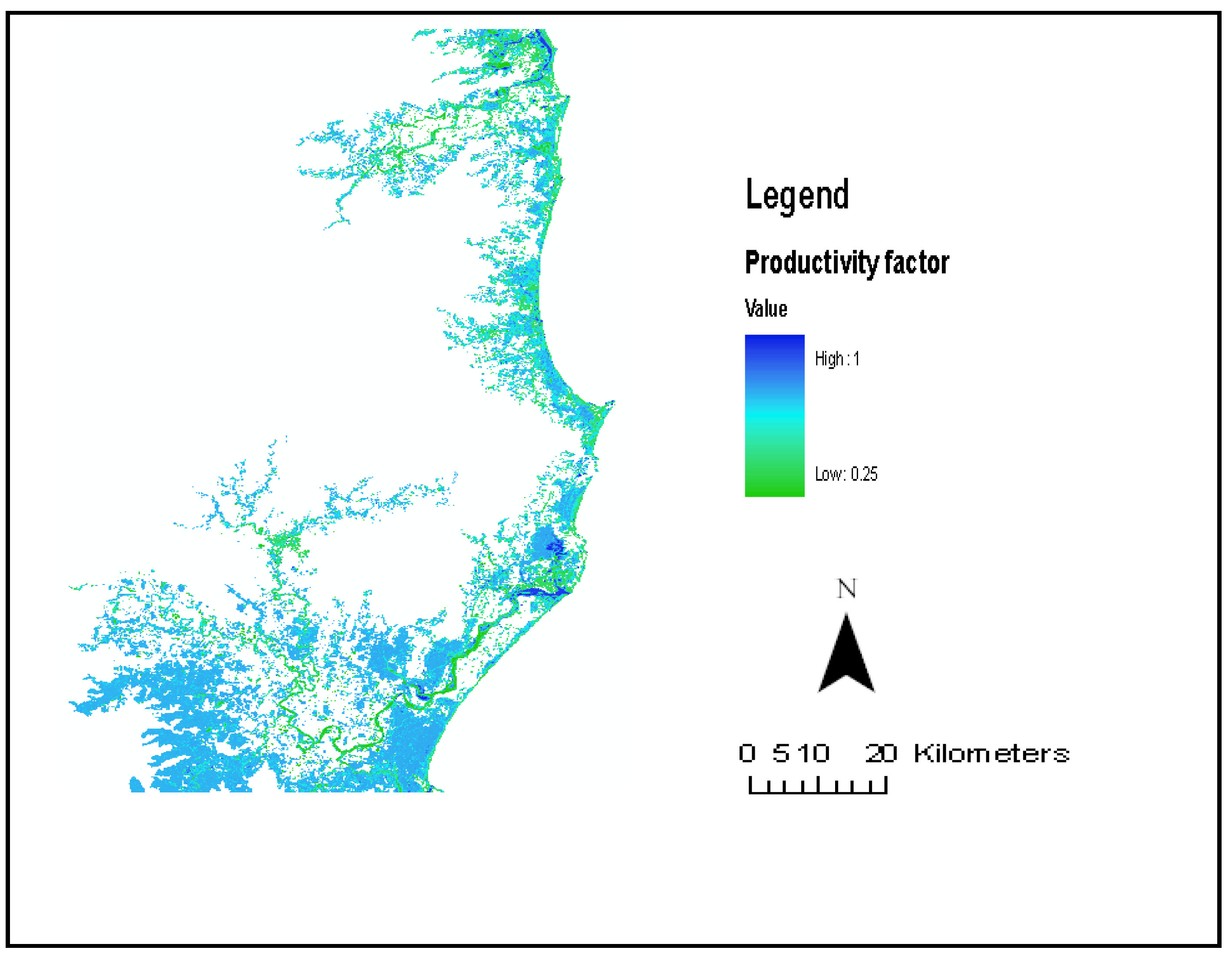
2.3.4. Productivity Factor

The productivity factor was a ratio of net primary productivity for each wetland ecosystem to net primary productivity of tropical rainforest (Equation 12) assuming that methane production in a tropical rainforest is constant throughout the year because of relatively constant temperatures and rainfall [29], i.e.,
R = NPP   ( ecosystem ) NPP   ( tropical   rainforest )
where:
  • R = Productivity factor
  • NPP = Net primary productivity.
Mean productivity factors for the wetland ecosystems (Table 6) were calculated using their net primary productivity values for the wetland classes adopted from [29,40]. The net primary productivity of the wetland types were obtained from the dry weight of above ground biomass.

2.3.5. Precipitation and Evaporation Ratio

Precipitation and evaporation values were obtained from the climate statistics in the region. This study assumes water saturation in the soil as a function of precipitation and evaporation ratio. A higher precipitation relative to evaporation is assumed that the soils are water saturated for a given period and a value of 1 is assigned for every grid cell. The mean precipitation and standard error (SE) in the month of June 2001 for the study area was 166.2 ± 26.7 mm while the mean evaporation and standard error for the month of June 2001 was 125 ± 35.4mm. The precipitation and evaporation ratio was therefore set to 1 for every grid cell.

3. Results

The maximum observed mean NDVI value of 0.685 ± 0.054 was for forested wetlands while coastal swamps had the minimum mean NDVI value of 0.565 ± 0.095 (Figure 4).
Figure 4. NDVI values of wetland vegetation in north-eastern NSW, Australia.
Remotesensing 02 01378 g004
The land surface temperature values (Figure 5) in the winter month of June 2001 were found to be higher in water than on land.
Figure 5. Estimated Land surface temperature (LST).
Remotesensing 02 01378 g005
The study identified and mapped the following wetland classes after the supervised classification: mangroves and saltmarshes, forested wetlands, coastal upland water bodies, estuarine water bodies, coastal swamps and dunal wetlands (Figure 6).
Figure 6. Wetland Classification in north-eastern NSW, Australia- Landsat ETM+, June 2001.
Remotesensing 02 01378 g006
The maximum T factor values (Figure 7) were found in estuarine water bodies, while forested wetlands had the minimum T factor values.
Figure 7. T Factor values for the wetland classes.
Remotesensing 02 01378 g007
Table 4. T factor and standard errors for the wetland classes.
WetlandT factorProjected T factor-assuming 1 °C rise in mean annual temperature by the year 2030
Mangroves and saltmarshes0.69 ± 0.150.96 ± 0.20
Forested wetlands0.45 ± 0.080.64 ± 0.12
Coastal swamps0.57 ± 0.160.80 ± 0.22
Estuarine water bodies1.03 ± 0.251.44 ± 0.34
Coastal upland water bodies0.71 ± 0.190.99 ± 0.26
Dunal wetlands0.70 ± 0.180.98 ± 0.25
Forested wetlands had the highest daily mean methane flux of 1.029 ± 0.01 g/m2/day while coastal upland water bodies had the least mean daily methane flux of 0.015 ± 0.004 g/m2/day.
Table 5. Estimated mean methane fluxes for the wetland classes.
Wetland classMean Flux ± SE (g/m2/day)Mean Flux ± SE (g/m2/month)Number of gas samples
Mangroves and saltmarshes0.016 ± 0.010.496 ± 0.3216
Forested wetlands1.029 ± 0.0131.286 ± 2.9716
Coastal swamps0.161 ± 0.054.893 ± 1.4416
Estuarine water bodies0.022 ± 0.00010.683 ± 0.00416
Coastal upland water bodies0.015 ± 0.0040.461 ± 0.1316
Dunal wetlands0.037 ± 0.021.123 ± 0.5416
The productivity factor (Figure 8) was highest in mangroves and saltmarshes while coastal upland water bodies had the lowest productivity factor.
Figure 8. Productivity factor of methane emission for the wetland classification.
Remotesensing 02 01378 g008
Table 6. Mean productivity factors and standard error for the wetland classes.
Wetland classMean Productivity factor and SE
Mangroves and saltmarshes1.00 ± 0.00
Forested wetlands0.73 ± 0.04
Coastal swamps0.75 ± 0.70
Estuarine water bodies0.95 ± 0.07
Coastal upland water bodies0.25 ± 0.00
Dunal wetlands0.39 ± 0.13
The maximum mean thermal emissivity value (0.992 ± 0.004) was for forested wetlands while coastal swamps had the minimum thermal emissivity value of 0.983 ± 0.009 (Figure 9).
Figure 9. Thermal emissivity values for the wetland classes.
Remotesensing 02 01378 g009
The accuracy assessment carried out for the wetland classification (Table 7) showed a maximum user's accuracy (96.15%) for mangroves and saltmarshes and the minimum user's accuracy (78.00%) for forested wetlands.
Table 7. Error Matrix Table for Landsat TM + 2001 wetland classification. Remotesensing 02 01378 i001
Producer’s AccuracyUser’s AccuracyOverall AccuracyOverall Kappa Statistics
D = Dunal wetlands85.19%90.20%
F = Forested wetlands79.59%78.00%
S = Coastal swamps84.62%83.02%
L = Coastal upland water bodies89.58%86.00%
M = Mangroves and saltmarshes98.03%96.15%
E = Estuarine water bodies87.93%91.07%
87.50%85.00%
The study also found forested wetlands to have the highest amount of methane emission (0.0016 ± 0.00009 Tg) in the month of June, 2001 while coastal upland water bodies had the minimum amount of methane emission (0.0000019 ± 0.0000005 Tg) in the month of June, 2001 (Table 8). According to the IPCC [4] report, the mean annual temperature will rise by 0.2 to 1.6 °C by the year 2030. In line with the IPCC [4] projection, an estimation of methane emission from the various wetlands by the year 2030, assuming 1 °C rise in mean annual temperature was projected to increase in the month of June (Table 8).
Table 8. Methane emitting areas and emission estimates in the month of June 2001 including mean annual temperature increase by 10C in north-eastern NSW, Australia.
Wetland typeArea covered by wetland (km2)Methane emission estimate in June (Tg) ± SEMethane emission estimate (Tg) in June assuming a 1 °C rise in mean annual temperature ± SE
Mangroves and saltmarshes36.560.000013 ± 0.0000060.000018 ± 000008
Forested wetlands152.090.0016 ± 0.000090.0022 ± 0.0001
Coastal upland water bodies32.740.0000019 ± 0.00000050.0000037 ± 0.0000007
Estuarine water bodies35.970.000024 ± 0.00000010.000034 ± 0.0000001
Coastal swamps150.560.00031 ± 000020.00044 ± 0.00001
Dunal wetlands73.370.000022 ± 0.0000080.000031 ± 0.00001
Total481.290.0019 ± 0.00010.0027 ± 0.0002

4. Discussion

The higher land surface temperature values found in water than on land in the winter month of June 2001 is probably due to the fact that in winter, water would absorb solar energy and hold onto heat longer than land. The possibility of using land surface temperature in estimating water table depth is an area of further research. Thermal emissivity of the wetlands was used to correct the spectral emissivity of the blackbody temperature generated. The high thermal emissivity value for forested wetlands was due to their high NDVI values. Nevertheless, there would be variation of the thermal emissivity values for the wetlands especially within seasons. This is because the NDVI values are likely to change with seasons due to changes in environmental conditions and the resulting foliage replacement and flowering cycles of the plants.
The higher T factor values found in estuarine water bodies was due to the higher temperatures found in estuarine waters at the time of satellite image acquisition. There would, however, be uncertainties in the T factor values due to the fluctuation in land surface temperatures within days, months, seasons and years. There were also variations in the productivity factor of the wetlands for methane emission. This is because it is dependent on the net primary productivity of the wetlands, which further depends on the variables such as vegetation, hydrology, climate, soil type and nutrients availability [40]. The area covered by the wetlands also contributed to the estimated amount of methane emission. Forested wetlands had the maximum amount of methane emission due to a large area and methane flux. The estimation of area covered by the wetlands was limited to the satellite data used and the environmental conditions of the wetlands at the time of image acquisitions. This is because the spatial resolution of the satellite data would influence the area covered by the wetlands and conditions such as floods and tides would also influence the wetland area. High tides would likely affect the area covered by estuarine water bodies, mangroves and saltmarshes due to their proximity to the sea. The estimated amount of methane emission from the wetlands classes was also influenced by their methane fluxes, which were obtained from field and lab experiments. The methane fluxes observed from mangroves and estuarine water bodies in this study were lower than the calculated mean methane fluxes of 7.38 mg/m2/hr for Pichavaram mangrove and 15.41 mg/m2/hr for Adyar estuary in south India [41]. The lower methane fluxes observed in mangrove sediments maybe a result of out-competition for substrates [42] by sulfate reducers. This is because in marine environments with high salinity, methanogenesis may be inhibited by sulfate-reducing bacteria [43,44]. Forested wetlands generally had a higher methane flux compared to the estimated 23.5 ± 11.3 g/m2/yr for forested wetland ecosystems calculated globally in Sheppard [29].
The variability of methane flux was high in the wetlands, especially in the forested wetlands. The uncertainties in methane flux were probably due to the changing environmental conditions such as soil temperature, rate of methane oxidation in the oxic soil between water table and soil surface and the difference in substrate availability. An increase in environmental conditions such as temperature and soil moisture content would increase methane flux from wetlands and vice versa [39]. Methane fluxes from wetlands would furthermore be affected by seasonal conditions. This is because there are different seasonal conditions of variables such as rainfall, temperature, evaporation and vegetation types, thereby increasing the variability of methane flux in a year.
The study assumed that methane emission processes from wetlands depend linearly on temperature due to the fact that methanogenic activities are influenced by soil temperature. It further assumed soil moisture content based on the ratio of precipitation and evaporation within a region, which is, however, limited to the availability of climate data. In addition, it assumed the mean methane fluxes measured from the various wetlands as a representative of the daily mean for each wetland type. This would nonetheless change with changing environmental conditions. However, in order to estimate annual methane emission from the wetlands it is imperative to model methane fluxes for the various seasons. This is because methane emission is expected to change throughout the year due to changes in parameters such as precipitation, and temperatures during winter, summer, autumn and spring. During summer with high temperatures, methane emission is likely to increase but this could be limited by a high rate of evaporation thereby reducing the area covered by wetlands. Methane emission would increase in autumn due to high rainfall, thereby increasing wetland area and soil moisture content. During spring and winter, methane emission from wetlands would decrease due to less rainfall and lower temperatures in the north-eastern region of NSW, Australia. Nevertheless, there is a further limitation in the estimation of annual methane emission from wetlands using satellite data. This includes the lesser availability of cloud free satellite images on a monthly basis which is necessary in order to acquire wetlands information such as area cover and quality for methane estimation.
Climate change (temperature increase) would probably increase natural methane emission from global wetlands. Policies geared towards carbon sequestration and storage could offset climate change and its impact to methane emission. The mitigation of methane emission from wetlands to the atmosphere is an area for further research. Remote sensing could play a vital role in identifying and monitoring the wetlands, and the acquisition of biophysical properties which could be used to improve our understanding of methane emission over time.

5. Conclusions

An estimation of methane emission from wetlands has been carried out using Landsat ETM+. This was modeled using the following parameters: productivity factor, temperature dependent factor (T-factor), wetland area, methane flux, precipitation and evaporation ratio. The estimation of methane emission from the wetlands has been carried out assuming methane production is linearly dependent on temperature. The study found a high variability of methane emission from the wetlands with the maximum amount of methane emission from forested wetlands and the minimum amount of emission from coastal upland water bodies. Methane emission is anticipated to increase with climate change which is most likely due to an increase in metabolic activities of the soil microbes. There are however uncertainties in the methane emission estimation due to changes in methane fluxes and environmental conditions such as temperature and rainfall over time from the wetlands. There are also limitations in the use of satellite data to estimate methane emission from wetlands such as the limitation in acquiring cloud free satellite images especially on a monthly basis and the factor of scale (spatial resolution) in delineating the wetland classes. Nevertheless, the empirical methane emission model using Landsat ETM+ is suitable to estimate monthly and yearly methane budget from wetlands at both local and regional level.

Acknowledgements

We would like to acknowledge the field support received from Paul Kelly and the assistance received from Dirk Erler, Joanne Oakes and Greg Luker at Southern Cross University. This work is supported from funding obtained from the Australian Government and Southern Cross University.

References

  1. What Are Wetlands? Ramsar Convention of Wetlands; Information Paper No. 1; Ramsar, Iran, 1971a.
  2. Mortsch, L.D. Assessing the impact of climate change on the great lakes shoreline wetlands. Climate Change 1998, 40, 391–416. [Google Scholar] [CrossRef]
  3. Hein, R.; Crutzen, P.J.; Heimann, M. An inverse modelling approach to investigate the global atmospheric methane cycle. Global Biogeochem. Cycle. 1997, 11, 43–76. [Google Scholar] [CrossRef]
  4. IPCC. Climate Change 2007. The Physical Science Basis; Contribution of Working Group I to the Fourth Assessment Report of the Intergovernmental Panel on Climate Change, Cambridge University Press: Cambridge, UK and New York, NY, USA, 2007. [Google Scholar]
  5. IPCC. Climate Change 2001. The Scientific Basis; Contribution of Working Group I to the Third Assessment Report of the International Panel on Climate Change, Cambridge University Press: Cambridge, UK, 2001. [Google Scholar]
  6. Lelieveld, J.; Crutzen, P.J.; Dentener, F.J. Changing concentration, lifetime and climate forcing of atmospheric methane. Tellus Series B 1998, 50, 128–150. [Google Scholar] [CrossRef]
  7. Hamazaki, T.; Kaneko, Y.; Kuze, A. Carbon dioxide monitoring from the GOSAT satellite. In Proceedings XXth ISPRS Conference, Istanbul, Turkey, 12–23 July 2004; p. 3.
  8. Asner, G.P. Cloud cover in Landsat observations of the Brazilian Amazon. Int. J. Remote Sens. 2001, 22, 3855–3862. [Google Scholar] [CrossRef]
  9. Baker, C.; Lawrence, R.; Montagne, C.; Patten, D. Mapping wetlands and riparian areas using Landsat Etm+ Imagery and decision-tree-based models. Wetlands 2006, 26, 465–474. [Google Scholar] [CrossRef]
  10. Lowry, J.; Hess, L.; Rosenqvist, A. Mapping and monitoring wetlands around the world using ALOS PALSAR: The ALOS kyoto and carbon initiative wetlands. In Innovations in Remote Sensing and Photogrammetry; Jones, S., Reinke, K., Eds.; Springer: Berlin/Heidelberg, Germany, 2009. [Google Scholar]
  11. Lucas, R.M.; Bunting, P.; Clewley, D.; Proisy, C.; Filho, P.W.M.S.; Woodhouse, I.; Ticehurst, C.; Carreiras, J.; Rosenqvist, A.; Accad, A.; Armston, J. Characterisation and Monitoring of Mangroves Using ALOS PALSAR Data; K&C Phase-1 Report; ALOS K&C: Kyoto, Japan, 2009. [Google Scholar]
  12. Allen, D.E.; Dalal, R.C.; Rennenberg, H.; Meyer, R.L.; Reeves, S.; Schmidt, S. Spatial and temporal variation of nitrous oxide and methane flux between subtropical mangrove sediments and the atmosphere. Soil Biol. Biochem. 2007, 39, 622–631. [Google Scholar] [CrossRef]
  13. Bohn, T.J.; Lettenmaier, D.P.; Sathulur, K.; Bowling, L.C.; Podest, E.; McDonald, K.C.; Friborg, T. Methane emissions from western Siberian wetlands: heterogeneity and sensitivity to climate change. Environ. Res. Lett. 2007, 2. [Google Scholar] [CrossRef]
  14. Liu, Y. Modelling the Emission of Nitrous Oxide (N2O) and Methane (CH4) from The Terrestrial Biosphere to the Atmosphere; Report No. 10; MIT Joint Program on the Science and Policy of Global Change: Cambridge, MA, USA, 1996. [Google Scholar]
  15. Xu, H.; Cai, Z.C.; Tsuruta, H. Soil moisture between rice-growing seasons affects methane emission, production, and oxidation. Soil Sci. Soc. Amer. J. 2003, 67, 1147–1157. [Google Scholar] [CrossRef]
  16. Kreuzwieser, J.; Buchholz, J.; Rennenberg, H. Emission of methane and Nitrous Oxide by Australian Mangrove Ecosystems. Plant Biol. 2003, 5, 423–431. [Google Scholar] [CrossRef]
  17. Kingsford, R. GIs of wetlands in the Murray-Darling Basin. WetlandCare Australia: Ballina, Australia. Available online: http://www.wetlandcare.com.au/Content/templates/research_detail.asp?articleid=106&zoneid=17 (accessed on 3 March, 2010).
  18. Agarwal, R.; Garg, J.K. Methane emission modelling using MODIS thermal and optical data: A case study on Gujarat. J. Indian Soc. Remote Sens. 2007, 35. [Google Scholar] [CrossRef]
  19. Takeuchi, W.; Tamura, M.; Yasuoka, Y. Estimation of methane emission from West Siberian wetland by scaling technique between NOAA, AVHRR and SPOT HRV. Remote Sens. Environ. 2003, 85, 21–29. [Google Scholar] [CrossRef]
  20. Hennessy, K.; Page, C.; McInnes, K.; Jones, R.; Bathols, J.; Collins, D.; Jones, D. Climate Change in New South Wales; Consultancy Report for the New South Wales Greenhouse Office, New South Wales Greenhouse Office: Sydney, NSW, Australia, 2004. [Google Scholar]
  21. Hilbert, D.W.; Ostendorf, B.; Hopkins, M.S. Sensitivity of tropical forests to climate change in the humid tropics of north Queensland. Austral Ecol. 2001, 26, 590–603. [Google Scholar] [CrossRef]
  22. Morand, D.T. Soils Landscapes of the Woodburn 1:100,000 Sheet Map; Department of Land and Water Conservation: Sydney, NSW, Australia, 2001.
  23. Morand, D.T. Soils Landscapes of the Lismore-Ballina 1:100,000 Sheet Map; Department of Land and Water Conservation: Sydney, NSW, Australia, 1994.
  24. Morand, D.T. Soils Landscapes of the Murwillumbah-Tweed Heads 1:100,000 Sheet Map; Department of Land and Water Conservation: Sydney, NSW, Australia, 1996.
  25. BOM. Climate statistics for Australian Locations. Available online: http://www.bom.gov.au/climate/averages/tables/cw_058065.shtml (accessed on 28 March, 2010).
  26. Green, D.L. Wetland classification. In Wetland Management Technical Manual: Wetland Classification; Ecological Services Unit: Sydney, NSW, Australia, 1997. [Google Scholar]
  27. Van de Griend, A.A.; Owe, M. On the relationship between thermal emissivity and the normalized difference vegetation index for natural surfaces. Int. J. Remote Sens. 1993, 14, 1119–1131. [Google Scholar] [CrossRef]
  28. Burrows, J.P.; Blyth, E.; Buchwitz, M.; Schneising, O. Methane from boreal wetlands: some issues. Available online: http://dup.esrin.esa.int/stse/files/news/J.%20Burrows%20-%20Methane%20from%20Boreal%20Wetlands%20-%20Some%20Issues.pdf (accessed on 3 March, 2010).
  29. Sheppard, J.C.; Westberg, H.; Hopper, J.F. Inventory of global methane sources and their production rates. J. Geophys. Res. 1982, 87, 1305–1312. [Google Scholar] [CrossRef]
  30. Mather, P.M. Computer Processing of Remotely-Sensed Images, 2nd ed.; John Wiley and Sons: Chichester, England, 1999. [Google Scholar]
  31. Archard, F.; D’Souza, G. Collection and Pre-Processing of NOAA-AVHRR 1 km Resolution Data for Tropical Forest Resource Assessment; Report EUR 16055; European Commission: Luxembourg, 1994. [Google Scholar]
  32. Eva, H.; Lambin, E.F. Burnt area mapping in Central Africa using ATSR data. Int. J. Remote Sens. 1998, 19, 3473–3497. [Google Scholar] [CrossRef]
  33. Ozesmi, S.L.; Bauer, M.E. Satellite remote sensing of wetlands. Wetlands Ecology Management 2002, 10, 381–402. [Google Scholar] [CrossRef]
  34. Congalton, R.G.; Green, K. Assessing the Accuracy of Remotely Sensed Data: Principles and Practices; Lewis Publishers, CRC Press: Boca Raton, FL, USA, 1999. [Google Scholar]
  35. Campbell, J.B. Introduction to Remote Sensing, 4rd ed.; Guilford Press: New York, NY, USA, 2006. [Google Scholar]
  36. LPSO. Landsat 7 Science Data User’s Handbook; Landsat Project Science Office, NASA: Greenbelt, MD, USA. Available online: http://landsathandbook.gsfc.nasa.gov/handbook/handbook_toc.html (accessed on 12 August, 2009).
  37. Snyder, W.C.; Wan, Z.; Zhang, Y.; Feng, Y.Z. Classification based emissivity for land surface temperature measurement from space. Int. J. Remote Sens. 1998, 19, 2753–2774. [Google Scholar] [CrossRef]
  38. Dinh, H.T.M.; Trung, L.V.; Van, T.T. Surface emissivity in determining land surface temperature. In The International Symposium on Geoinformatics for Spatial-Infrastructure Development in Earth and Applied Sciences(GIS-IDEAS), Vietnam, 9–11 November, 2006.
  39. Wang, Y.; Wang, Y. Quick measurement of CH4, CO2, and N20 emissions from a short plant ecosystems. Adv. Atmos. Sci. 2003, 20, 842–844. [Google Scholar]
  40. Cronk, J.K.; Fennessy, M.S. Wetland Plants: Biology and Ecology; Lewis Publishers: New York, NY, USA, 2001. [Google Scholar]
  41. Purvaja, R.; Ramesh, R. Natural and anthropogenic methane emission from coastal wetlands of South India. Environ. Manag. 2001, 27, 547–557. [Google Scholar] [CrossRef]
  42. Lovely, D.R.; Klug, M.J. Sulphate reducers can outcompete methangens at fresh water sulphate concentrations. Appl. Environ. Microbiol. 1983, 45, 187–192. [Google Scholar]
  43. Abram, J.W.; Nedwell, D.B. Hydrogen as a substrate for methanogenesis and sulphate reduction in anaerobic saltmarsh sediment. Arch. Microbiol. 1978, 117, 89–92. [Google Scholar] [CrossRef] [PubMed]
  44. Verma, A.; Subramanian, V.; Ramesh, R. Methane emission from coastal lagoon:Vembanad lake, west coast India. Chemosphere 2002, 47, 883–889. [Google Scholar] [CrossRef]

