Change Detection Accuracy and Image Properties: A Study Using Simulated Data

Abstract

Simulated data were used to investigate the relationships between image properties and change detection accuracy in a systematic manner. The image properties examined were class separability, radiometric normalization and image spectral band-to-band correlation. The change detection methods evaluated were post-classification comparison, direct classification of multidate imagery, image differencing, principal component analysis, and change vector analysis. The simulated data experiments showed that the relative accuracy of the change detection methods varied with changes in image properties, thus confirming the hypothesis that caution should be used in generalizing from studies that use only a single image pair. In most cases, direct classification and post-classification comparison were the least sensitive to changes in the image properties of class separability, radiometric normalization error and band correlation. Furthermore, these methods generally produced the highest accuracy, or were amongst those with a high accuracy. PCA accuracy was highly variable; the use of four principal components consistently resulted in substantial decreased classification accuracy relative to using six components, or classification using the original six bands. The accuracy of image differencing also varied greatly in the experiments. Of the three methods that require radiometric normalization, image differencing was the method most affected by radiometric error, relative to change vector and classification methods, for classes that have moderate and low separability. For classes that are highly separable, image differencing was relatively unaffected by radiometric normalization error. CVA was found to be the most accurate method for classes with low separability and all but the largest radiometric errors. CVA accuracy tended to be the least affected by changes in the degree of band correlation in situations where the class means were moderately dispersed, or clustered near the diagonal. For all change detection methods, the classification accuracy increased as simulated band correlation increased, and direct classification methods consistently had the highest accuracy, while PCA generally had the lowest accuracy.

1. Introduction

The monitoring and evaluation of environmental change is one of the major applications of remote sensing. As a consequence, a large and growing literature has focused specifically on change detection methods [1], resulting in a proliferation of proposed approaches. Despite this focus on change detection analysis, a consensus regarding the relative benefit of even the main change detection methods has not emerged. Partly, this is because many of the studies that have compared change detection methods have reached different conclusions. It is notable that most change detection comparison studies are focused on case studies of a single region.

It is our hypothesis that, because the different change detection methods involve different image processing methods, differences in the images used in the case studies may at least in part explain the apparently contradictory results regarding the relative merits of the different methods [2]. In this paper we therefore seek to evaluate whether image properties affect the relative change detection classification accuracy for five commonly used change detection methods. Our approach is based on simulated data, rather than real data, because with simulated data we can completely control image properties, and also evaluate accuracy with absolute reliability. We are therefore able to test the different methods with great consistency over a wide range of image properties.

The three image properties investigated in this paper are radiometric normalization, spectral separability of the classes of interest, and correlation between the spectral bands. The importance of radiometric normalization for accurate change detection has been discussed extensively in previous studies [3,4,5]. Radiometric normalization is required because there may be (a) differences between the images due to changes in illumination due to variation in sun-earth distance, solar azimuth or zenith angle, (b) changing atmospheric conditions causing differing scattering and absorption, and (c) sensor differences.

In comparison, there has been little discussion on the influence on change detection due to the multispectral separability of the spectral classes and the relative correlation of the individual image bands. Nevertheless, to the extent that change detection is conceptualized as a classification problem, image spectral properties should be of great importance.

Other image properties, particularly the combination of image spatial heterogeneity and spatial misregistration, also play an important role in determining change detection classification accuracy [6,7,8,9,10], and likely affect the relative accuracy of different change detection methods [11]. However, for this study we focus exclusively on spectral properties.

This article is structured in seven major sections. Following this introduction, a brief overview of five common change detection methods is presented in the second section, followed by a discussion of prior studies on the relative accuracies of the different change detection methods. In the fourth section, the experimental methods are described, focusing particularly on the construction and testing of the simulated data. In the fifth section the results are presented. This is followed be a discussion in Section 6, and general conclusions are drawn in Section 7.

2. Overview of Change Detection Methods

The five methods discussed here represent on aggregate some of the most commonly used and straight-forward change detection methods. Each method is described individually below, and in the following section we present a discussion of the relative accuracies of the methods as suggested by previous studies.

2.1. Post-Classification Comparison

Post-classification comparison is conceptually one of the most simple change detection methods. The method involves an initial, independent classification of each image, followed by a thematic overlay of the classifications. The method results in a complete “from-to” change matrix of the transitions between each class on the two dates. One issue with this method, less frequently commented on, is the importance of producing consistent classifications for each of the independent classifications. Specifically, the error in post-classification change detection is greatest when the errors in each classification are uncorrelated with each other, and lowest when the errors are strongly correlated between the two dates [12]. One possible method for increasing the likelihood of producing the most similar classification is to normalize the two images radiometrically, and then using the same training data for both classifications. A disadvantage with this approach is that it may introduce an additional source of error in the radiometric normalization step.

2.2. Direct Classification

Direct classification is similar to post-classification comparison, except that a single classification is undertaken, instead of two independent classifications [13,14]. The images from the two dates are first combined in a single composite layer-stack, and the composite data set classified to produce the final change map in a single step. The challenge with this method is that the number of potential change transitions is the square of the number of classes present for one particular date. Therefore, for supervised classification, the analyst needs to find training pixels to represent a potentially large number of change classes. Unsupervised classification also holds challenges for this method, because some of the change transitions may be too rare to generate distinctive spectral clusters. As with conventional post-classification comparison using separate training data for each date, no radiometric normalization is required.

2.3. Principal Component Analysis

Principal component analysis (PCA) is a commonly used data transformation method that has broad application in data compression and data exploration. PCA comprises a linear transformation of an n-band image to produce n new, uncorrelated principal component (PC) bands. The n PCs are ranked according to the proportion of the variance in the original image explained by each band. PCs with the highest rank, explaining the largest proportion of the original variance, are generally assumed to carry the most information. PC bands that have a low rank tend to concentrate noise in the data, especially noise uncorrelated between bands. In a change analysis, where PCA is applied to a single layer-stack combining the multispectral images of the two dates, it is assumed that the highest order band or bands will likely represent information that is unchanged between the two dates [15]. Change should be concentrated in the subsequent PCs, with noise dominating the lowest order PCs. This relatively simplistic interpretation should be used with caution because PCA is a scene-specific transformation. The representation of change in the various PCs will change with the proportion of pixels in an image undergoing change, and the spectral variability in each of the individual images. Thus, interpreting a PCA change analysis image can be a challenge. Nevertheless, PCA can be very effective, especially for visualization of the inherent spectral information, including change information in high-dimension data and data from multiple sensors [16].

2.4. Image Differencing

The subtraction of one image band of one date from the same image band of another date is known as image differencing [13]. In the differenced image, spectral changes are highlighted as relatively high positive or negative values. Unchanged pixels are associated with values close to zero, and therefore image differencing does not allow the differentiation of the classes that are unchanged between the two dates. Image differencing can be carried on a single band or multiple bands. It is a relatively simple approach, and therefore is commonly used. However, image differencing does require radiometric normalization.

2.5. Change Vector Analysis

Change vector analysis (CVA) separates spectral change into two components: (a) the overall magnitude of the change, and (b) the direction of change [17,18,19]. The magnitude of change is determined by constructing a vector in the multispectral feature space. The one end of the vector is specified by the multispectral digital numbers (DNs) for the first date, and the other end by the DN values for the same pixel on the second date. The magnitude of change is a scalar variable representing the length of the vector, and is assumed to be related to the degree of physical change on the ground. Thus CVA analysis can be useful for evaluating continuous change, such as a reduction in biomass, or an increase in soil moisture. For an image with two spectral features or bands, the direction of change is an angle between 0° and 360°, with different types of change tending to be associated with characteristic directions. CVA was originally conceived of as a method for analyzing two spectral dimensions [17], and was later extended to an unlimited number of dimensions [13,20,21].

3. Relative Accuracy of the Change Detection Methods

3.1. Empirical Studies

The notable feature of the empirical studies is the wide range of overall findings. A number of studies have found image differencing to be the method with the highest overall accuracy [22,23,24,25,26]. However, other studies start have found post-classification to be the most accurate change method [27], and some go as far as to assume it can be used as a standard for evaluating the results of other change methods [28]. Yet other studies have found direct classification and post-classification [23,29] to have the lowest accuracy. PCA has been found to have the highest accuracy [16,29,30], or close to the highest [24], but also has been observed to have the lowest accuracy of the methods evaluated [25].

Even the general conclusions that have been drawn appear contradictory. For example, some studies conclude that simple techniques, such as image differencing, tend to perform better than complex methods, such as principal component analysis and CVA [23,25]. However, others find CVA to be the most accurate technique [31].

3.2. Theoretical Studies

Of particular interest for this study are theoretical analyses that have evaluated the relative accuracy of different change detection approaches based on understanding of how the various methods. Castelli et al. [32] modeled the probability distributions associated with change and no change classes, and then evaluated the Baysian decision rules for post-classification and image differencing. Modeled error for image differencing was found to be much larger than for post-classification, suggesting the latter is inherently more accurate. Liu et al. [33] examined a number of approaches, including image differencing and PCA, from a theoretical perspective. By plotting the theoretical distributions of classes in bi-temporal feature space, and modeling the error propagation of each method, they conclude that PCA was one of the better methods studied, and that it should out-perform image differencing.

4. Methods

4.1. Scene Model and the Simulated Data Construction

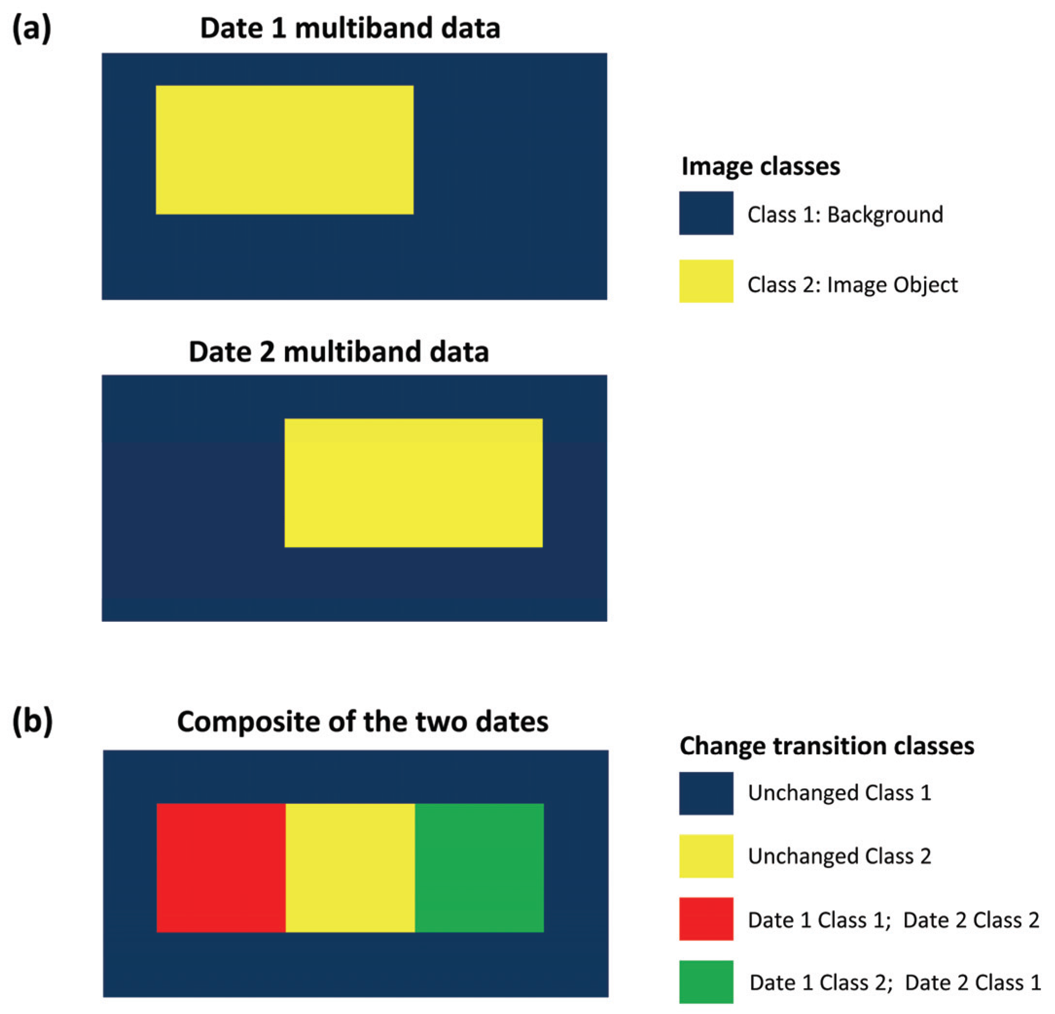
The simulated change images were constructed from a scene model consisting of three classes against a background class, resulting in a total of four classes. The first image was constructed directly from the scene model, and the second image, representing a later time period, was constructed by moving the boundaries of the classes in the scene model to represent the landscape change. Figure 1 is an overall schematic of the use of the simulated data in this study, illustrated using just one class in addition to the background.

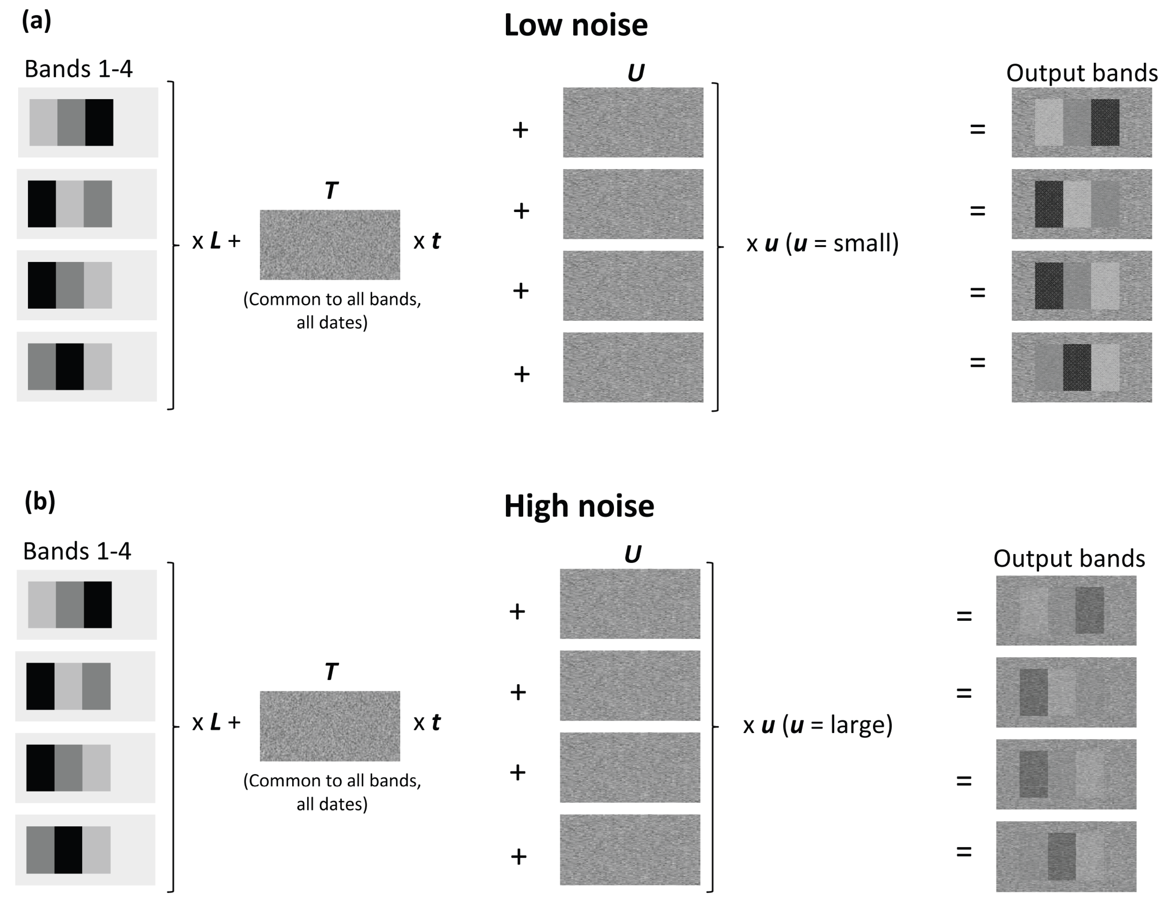
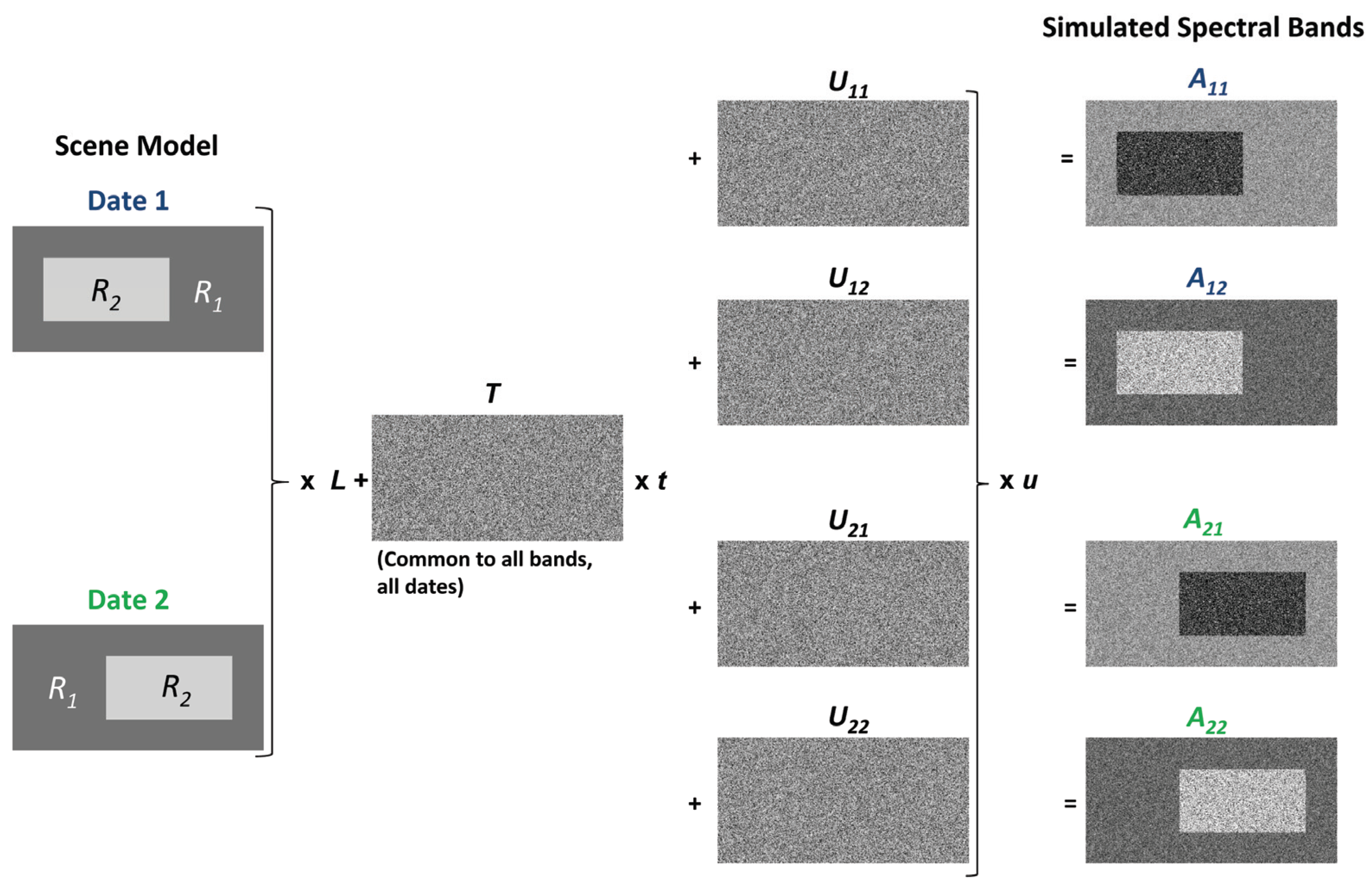
The construction of the simulated data is shown schematically in Figure 2. In the scene model, each class was assigned a distinctive spectral reflectance value, R_xc, where x is the spectral band and c is the class. R_xc is a real number between 0 and 1. T is the image texture that is present in all bands and represents variation in image brightness due to albedo differences and varying surface orientation with respect to the illumination. U is the simulated noise and uncorrelated class variability. T and U were generated as random images that have a Gaussian radiometric distribution, with a zero-mean and unit-standard deviation. T and U were radiometrically scaled by t and u, respectively. An illumination component, L, is represented by a constant for the entire scene and all bands, and was chosen to scale the data to an 8-bit range. Thus the simulated spectral image A_ix for time period i and spectral band x, is calculated:

Figure 1. Schematic illustration of simulated data for a two class situation. (a) The original data consists of multiband data sets. (b) When the images are combined, a multitemporal change image is produced.

Figure 1. Schematic illustration of simulated data for a two class situation. (a) The original data consists of multiband data sets. (b) When the images are combined, a multitemporal change image is produced.

Figure 2. Schematic outline of the process of construction of a two-class, two-band simulated data set.

Figure 2. Schematic outline of the process of construction of a two-class, two-band simulated data set.

A_ix = R_xc * L + T * t + U_ix * u

(1)

In developing the simulations, arbitrary values were chosen for the scaling parameters in order to ensure that a wide range of image properties were generated in the resulting image data set.

In the following subsections, the generation of data for the three classes of experiments is described in more detail.

4.1.1. Spectral Separability

For the first experiment, the analysis of the effect of spectral separability, four spectral bands were simulated for each time period (Figure 3). Four spectral bands allowed the generation of a more complex relationship between separability and the image bands than could be generated with just two bands, the number used in the subsequent experiments on radiometric normalization and band correlation.

Each of the four simulated cover classes was assigned a distinctive absorption feature in one of the four bands. The spectral separability between classes was varied by changing the spectral properties of noise (Figure 2) through the t and u parameters (Equation 1).

Average divergence and Jeffries Matusita (JM) distance summary class separability statistics were calculated for the simulated classes (Table 1). Divergence and JM distance both take into account the distance between class means and the difference between the covariance matrices of the classes [34]. However, divergence has no upper limit, whereas the JM distance is scaled between 0 and 2^0.5 (1.414), with a value of 2^0.5 indicating perfect separability. The JM distance is a particularly useful separability metric because it can be used to calculate the upper and lower bounds on the probability of classification error [34].

Table 1. Parameters used to construct simulated data and associated average class separability for change classes. See Equation (1) for definitions of t and u.

t	u	Divergence	JM Distance
0.8	0.3	451	1.414
1	0.5	968	1.414
3	1	301	1.414
5	2	79	1.414
7	3	36	1.406
1	4	20	1.356
6	5	13	1.264
8	6	9	1.159
15	7	7	1.057

Table 1. Parameters used to construct simulated data and associated average class separability for change classes. See Equation (1) for definitions of t and u.

t	u	Divergence	JM Distance
0.8	0.3	451	1.414
1	0.5	968	1.414
3	1	301	1.414
5	2	79	1.414
7	3	36	1.406
1	4	20	1.356
6	5	13	1.264
8	6	9	1.159
15	7	7	1.057

Figure 3. Overview of the construction of simulated data for a range of class separability through adjustments in band variability (noise). (a) Low noise. (b) High noise.

Figure 3. Overview of the construction of simulated data for a range of class separability through adjustments in band variability (noise). (a) Low noise. (b) High noise.

4.1.2. Radiometric Normalization

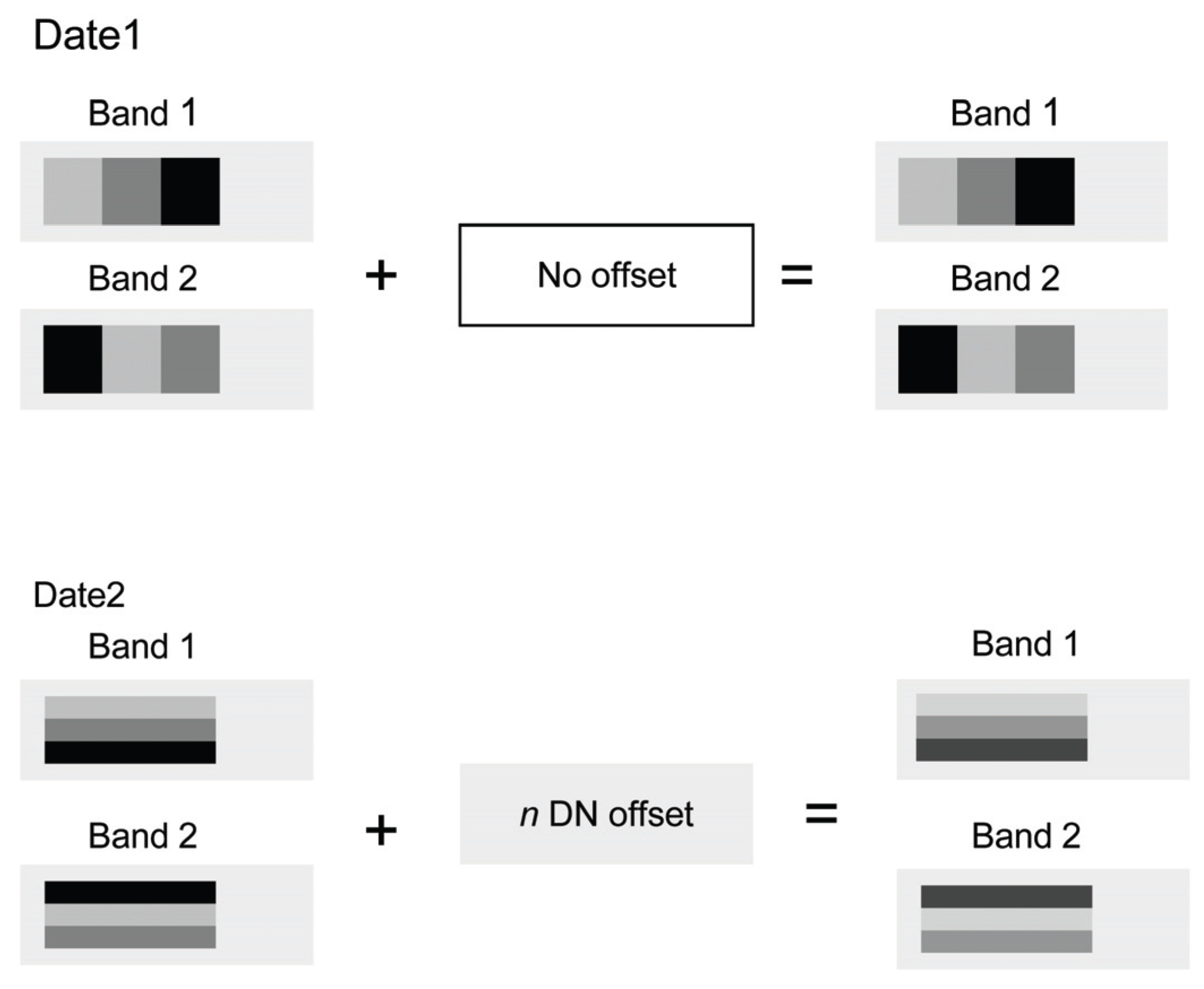
The radiometric normalization experiment was carried out using two bands of simulated data that discriminated the four cover types. Because of the increased number of cover types, a slightly modified spatial arrangement of the classes for the second date (Figure 4) was used in order to produce a change product in which all 16 change transitions were represented in a simple geometric arrangement. The effect of radiometric normalization error was simulated by adding a constant to each band of one of the image dates in each change image pair. The radiometric error value was varied from 0 to 10 DN, in 7 different simulations (Table 2). Because the importance of accurate radiometric normalization was hypothesized to be a function of the spectral separability of the classes, this experiment was replicated at three levels of class separability, varying from high (divergence = 250, JM distance = 1.386) to low (divergence = 16, JM distance = 1.113) separability (Table 3). Each pair of simulated images was classified using class signatures developed for the simulated data with no radiometric offset.

The two change detection techniques that require radiometric normalization, image differencing and change vector analysis, as well as post-classification using a single set of training data, were used for this experiment. The remaining two methods, PCA and direct classification, do not generally require radiometric normalization, and therefore were not used for this experiment.

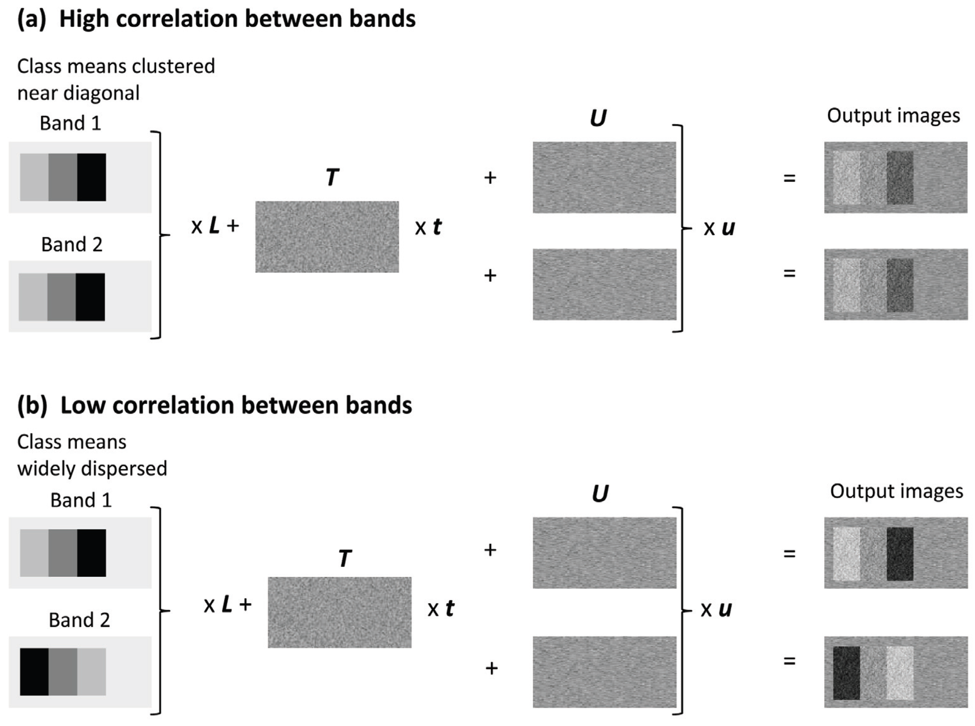
4.1.3. Band Correlation

Three tests were performed to examine the effect of band correlation on the accuracy of change detection techniques. Each test consisted of six simulations, with different levels of non-correlated noise (Table 4, Figure 5). The simulated reflectance values of the scene classes were modified between each test, to provide further differentiation in band correlation. The correlation between bands ranged from low, with class means widely dispersed within the feature space (i.e., the potential multivariate range of DNs), to high, with means clustered near the feature space diagonal. The t parameter, which controls the correlated variability between bands, was kept constant during these experiments.

Table 2. Offsets used in constructing the simulated data for the radiometric normalization experiment.

Offset value
0
2
3
5
7
10

Table 2. Offsets used in constructing the simulated data for the radiometric normalization experiment.

Offset value
0
2
3
5
7
10

Table 3. Parameters used to create the three groups of varying class separability for the radiometric normalization experiment.

t	u	Class separability	Divergence	JM Distance
7	3	High	250	1.386
10	7	Moderate	47	1.324
20	12	Low	16	1.113

Table 3. Parameters used to create the three groups of varying class separability for the radiometric normalization experiment.

t	u	Class separability	Divergence	JM Distance
7	3	High	250	1.386
10	7	Moderate	47	1.324
20	12	Low	16	1.113

Figure 4. Overview of the construction of the simulated data with radiometric error (offset) between dates. In this example, the DN values for date 2 are offset by a specified amount, n.

Figure 4. Overview of the construction of the simulated data with radiometric error (offset) between dates. In this example, the DN values for date 2 are offset by a specified amount, n.

Table 4. Parameters used to construct simulated data for the band correlation experiment.

Location of class means	T	U	Divergence	JM Distance	r
Clustered near diagonal	20	12	22	0.827	0.893
	20	6	82	0.976	0.952
	20	3	234	1.210	0.969
	20	1	2,690	1.392	0.973
Moderatelydispersed	20	12	25	1.197	0.818
	20	10	36	1.257	0.840
	20	7	72	1.345	0.867
	20	4	216	1.391	0.885
	20	2	846	1.392	0.892
Widely dispersed	20	18	15	1.177	0.631
	20	11	39	1.331	0.709
	20	3	184	1.391	0.752
	20	1	1,151	1.392	0.762

Table 4. Parameters used to construct simulated data for the band correlation experiment.

Location of class means	T	U	Divergence	JM Distance	r
Clustered near diagonal	20	12	22	0.827	0.893
	20	6	82	0.976	0.952
	20	3	234	1.210	0.969
	20	1	2,690	1.392	0.973
Moderatelydispersed	20	12	25	1.197	0.818
	20	10	36	1.257	0.840
	20	7	72	1.345	0.867
	20	4	216	1.391	0.885
	20	2	846	1.392	0.892
Widely dispersed	20	18	15	1.177	0.631
	20	11	39	1.331	0.709
	20	3	184	1.391	0.752
	20	1	1,151	1.392	0.762

Figure 5. Overview of the construction of the simulated data with varying degrees of correlation between bands. (a) Construction of an image with high correlation between bands (b) Construction of an image with low band-correlation.

Figure 5. Overview of the construction of the simulated data with varying degrees of correlation between bands. (a) Construction of an image with high correlation between bands (b) Construction of an image with low band-correlation.

As with the radiometric offset experiment, only two bands were used for each date, for the purpose of simplicity. All five change detection techniques were applied to the data.

4.2. Change Detection Analysis and Classification

The outcome of post-classification comparison and direct classification is a classified image; the product of the other change methods is an image. In order to facilitate quantifiable comparisons of the change analysis methods, the spectral change images were also classified. Maximum likelihood [34,35] was used for the classifications, with the exception of the CVA classification, for which a modified approach was employed, as will be explained below. Maximum likelihood was chosen because it is a powerful classifier for parametric data of the type generated in the simulated experiments.

For the post-classification comparison, training data were collected using the entire scene model as a template. Each image was classified separately and then overlaid.

The direct classification was undertaken by first combining the two dates into a single multi-date file, which was then input into the maximum likelihood classification. The training data for the direct classification was generated from an overlay of the scene models for the two dates that showed all possible change transitions.

Imaging differencing was carried out subtracting each band of the first date from the corresponding band of the image from the second date. The output image was written to a signed 16 bit file, and then classified.

For the PCA analysis, the multi-date image developed as an input for direct classification was used for calculating the PCs. The number of components to be calculated was set to the total number of bands in the multi-date file, 8. For the classification of the PCA change data, a subset of the PCA bands was used, since the purpose of PCA is normally to select a subset of variables to represent the information in the original multiband data set. Unfortunately, there is no standard specific choice of PCA bands, or even number of bands, suggested in the literature. Therefore, the classification was run twice, using the best four and six PCs, respectively, from the original 8 bands. The best PCs were defined as the PCs that appeared to display the most distinctive change patterns, and the choice was made based on a visual interpretation of the images. Because of the way the simulated data were constructed, the best four and six components were usually PCs 2 through 5 and 2 through 7, respectively. However, in some very noisy images, PC 8 was chosen over PC 7 because it had more spatial coherence.

For the CVA analysis, traditional two-band CVA classification was used. For the separability experiments, the four bands of data were projected to two dimensions using a modified PCA approach called multivariate spatial correlation (MSC) [36,37]. MSC is similar to PCA, except the eigenvectors are calculated from a matrix of multivariate spatial correlation values, instead of covariance values [36]. The MSC transformation is particularly effective for discriminating spatial patterns in the presence of uncorrelated noise [37].

The threshold discriminating change from no-change in the CVA magnitude data was selected directly from the training data using the probability density functions of the change and no-change classes [21]. The boundary between the two classes was then calculated as the angle where the two probabilities are equal:

$${\mathbf{B}}_{\mathbf{change},\mathbf{no}-\mathbf{change}}={\overline{\mathbf{X}}}_{\mathbf{change}}+\left(\frac{{\overline{\mathbf{X}}}_{\mathbf{change}}-{\overline{\mathbf{X}}}_{\mathbf{no}-\mathbf{change}}}{\mathsf{\sigma }{}_{\mathbf{change}}+\mathsf{\sigma }{}_{\mathbf{no}-\mathbf{change}}}\right){\mathsf{\sigma }}_{\mathbf{no}-\mathbf{change}}$$

(2)

• ${\mathbf{B}}_{\mathbf{change},\mathbf{no}-\mathbf{change}}$ = Boundary between change and no-change classes
• ${\overline{\mathbf{X}}}_{\mathbf{no}-\mathbf{change}}$ = mean of no-change class
• ${\overline{\mathbf{X}}}_{\mathbf{change}}$ = mean of change class
• $\mathsf{\sigma }{}_{\mathbf{no}-\mathbf{change}}$ = standard deviation of no-change class
• $\mathsf{\sigma }{}_{\mathbf{change}}$ = standard deviation of change class

The same approach employing probability density functions [21] was used for identifying the boundaries between the various change classes. Special care has to be taken in classifying classes with spectral angles near the discontinuity between 0° and 360°. This problem was addressed by rescaling the angles for classes on either side of the discontinuity to a continuous scale, using negative values or values greater than 360°, as needed.

4.3. Accuracy Evaluation

The classified change images were compared to the entire reference change image, generated from the original scene models, in order to evaluate the accuracy of each change detection method. By using the entire reference images for both training and accuracy assessment, questions of the sample size or representativeness of the training and accuracy data were avoided. This approach will likely result in optimistic accuracies compared to a typical real-world scenario where different testing and training data are normally used. However, since the focus of this study was relative accuracy, and not absolute accuracy, this was not regarded as a problem.

The accuracy of the change detection methods were analyzed in two groups. The first group comprises the techniques that differentiate the unchanged class into each of the cover types analyzed, which we refer to as comprehensive change analysis. Thus, for the simulated experiment with four cover types, twelve change classes and four unchanged classes are mapped, producing a sixteen-class comprehensive change analysis. Change detection methods that generate comprehensive change analysis include post-classification comparison, direct-classification and PCA. The second type of change analysis, partial change analysis, does not differentiate between unchanged cover classes. Thus for the four class simulated data, partial change analysis produces twelve change classes and one unchanged class, a total of thirteen classes. Change detection methods that produce only partial change analysis includes image differencing and CVA. To facilitate comparison between the methods associated with comprehensive and partial change analysis, the results of the comprehensive change analysis group were also collapsed to the smaller number of change classes associated with the partial change analysis. Because partial change analysis involves fewer classes, and is therefore a simpler classification problem, the overall accuracy may be higher than complete change analysis.

The results of the accuracy analysis were summarized by an overall accuracy percentage, and a kappa statistic. The kappa statistic provides a measure of the accuracy adjusted for chance agreement [38].

5. Results

5.1. Spectral Separability

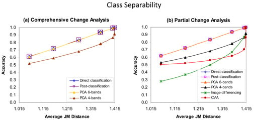
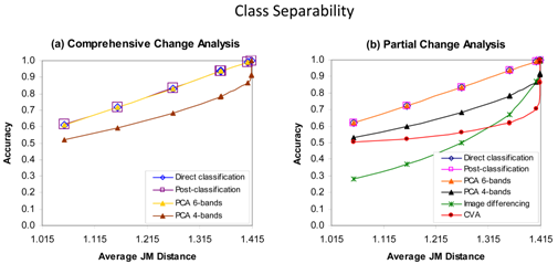
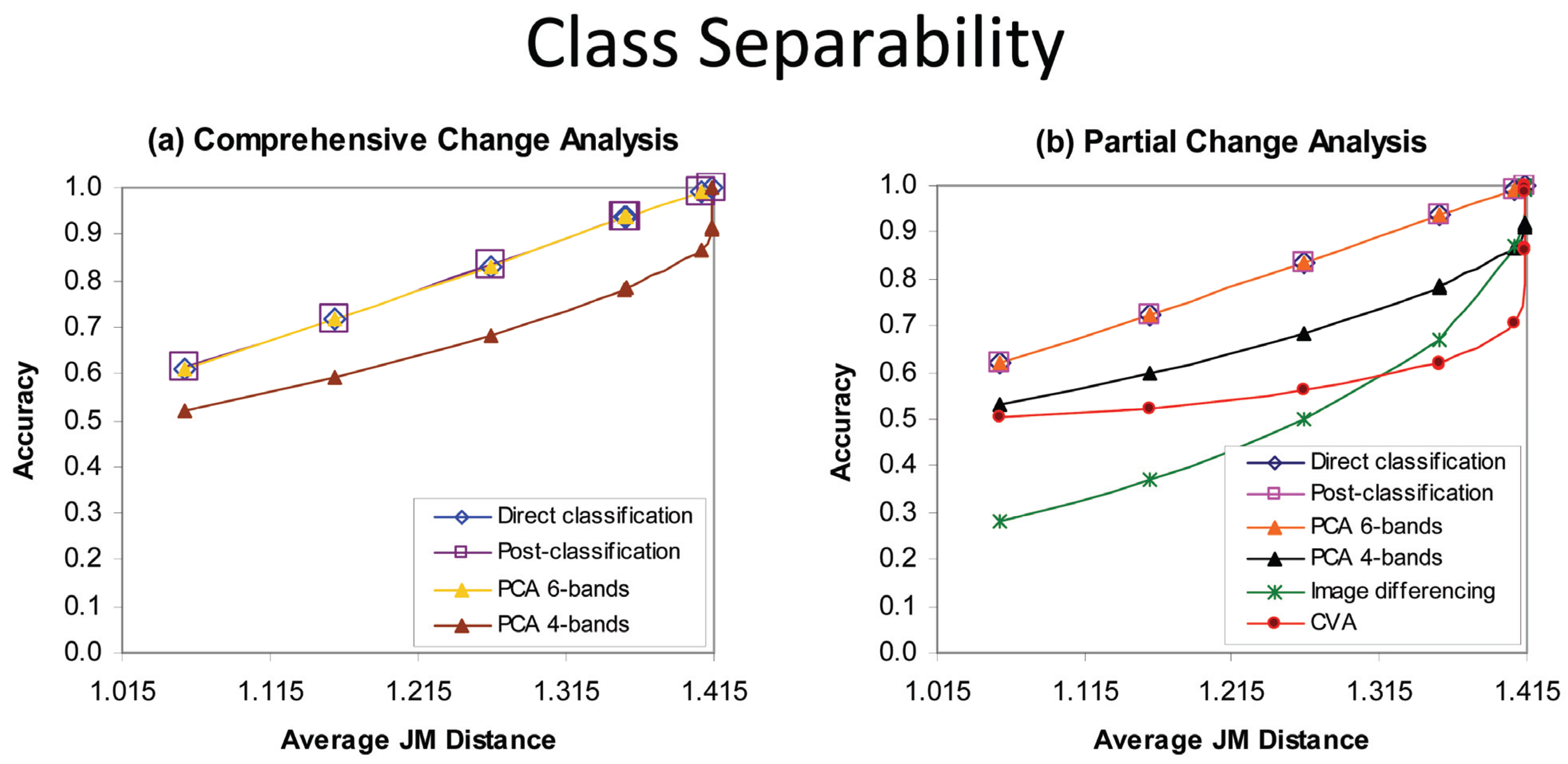
The first experiment was an analysis of the effect of spectral separability on change detection analysis accuracy, using images with four bands and four classes. The results are graphed in Figure 6, with the three comprehensive change approaches depicted separately (Figure 6(a)) from the five partial change methods (Figure 6(b)). As would be expected, the overall accuracy of change detection analysis is shown to be dependent on the spectral separability of the classes. Post-classification comparison, direct classification and PCA using the best six bands produced almost identical change detection accuracy. These three methods were consistently the most accurate, and showed a linear increase in accuracy with increasing class separability as measured by JM distance. The similarity in results was consistent for both comprehensive (Figure 6(a)) and partial change (Figure 6(b)) approaches. It is not surprising that direct classification produced accuracies similar to that of post-classification comparison, because these two methods are conceptually very similar, if perfect training data is available. The reason that the results of the six-band PCA change analysis was so similar to direct classification and post-classification comparison is that the PCA analysis effectively segregated the entire class information in the data in the first six principal components, and consequently the subsequent classification of the six-band PCA data was equivalent to classification using all eight original bands.

Figure 6. Effect of class spectral separability, measured by average divergence, on accuracy of comprehensive and partial change analysis methods, for the simulated data.

Figure 6. Effect of class spectral separability, measured by average divergence, on accuracy of comprehensive and partial change analysis methods, for the simulated data.

The four-band PCA change analysis produced a substantially lower accuracy, as much as 8–15%, over a wide range JM distances, compared to the equivalent six-band PCA change analysis, direct classification and post-classification comparison. In addition, four-band PCA required a divergence greater than 300, compared to a value greater than 50 for the six-band PCA, before 100% accuracy was reached (data not shown). The difference in accuracy between the four- and six-band PCA results suggests that potential accuracy of a PCA change analysis will be dependent on the number of principal components selected by the user, or more correctly, on the proportion of the information content of the multitemporal composite that is captured by the principal components used. Although the eigenvalues are usually assumed to be a good measure of the information content of the various bands, that assumption is not necessarily valid. For example, in the six-band PCA study, the accuracy obtained was similar to that obtained using all the data, despite the exclusion of the first PC, which by definition has the greatest eigenvalue of the principal components. In this case, however, the first PC isolated simulated illumination, which was not useful for discriminating the different change classes. An added complexity is that, for the very noisy data (low separability), the last principal component sometimes had less class differentiation information than the second last principal component.

The relationship between spectral separability and accuracy is complex for the four-band PCA, image differencing and CVA partial change analysis methods (Figure 6(b)). At low separabilities (JM 1.057 to 1.320, divergence up to 20), the relative rank of these three methods (in order of decreasing accuracy) is: four-band PCA, CVA and image differencing. For separabilities that are close to, or just reaching, complete separability (JM 1.320 to just less than 1.414, divergence 20 to 150), the relative rank is four-band PCA, image differencing and CVA. It is notable that CVA accuracy increased only slightly (by 0.12) as class separability increased over the range JM = 1.057 to 1.355, whereas four-band PCA improved by 0.26 and image differencing by 0.38. At high separabilities (JM =1.414, divergence 150–450), the relatively rank is image differencing, CVA, four-band PCA-4. Image differencing reaches 99% accuracy first, at a divergence of approximately 80, then CVA at a divergence of approximately 301, and only at a divergence value of 451 does the four-band PCA achieve a completely accurate classification.

In summary, in the class separability experiments, post-classification comparison, direct classification and six-band PCA gave the highest accuracy at all class separations, and for these methods, class separability as measured by the JM distance was almost linearly related to change detection accuracy. CVA, four-band PC and image differencing produced lower accuracies than post-classification comparison, direct classification and six-band PCA. For moderate to low class separabilities, CVA was relatively insensitive to class separability. The accuracy of image differencing relative to CVA and four-band PCA changed from lowest to highest, as separability increased.

5.2. Radiometric Normalization

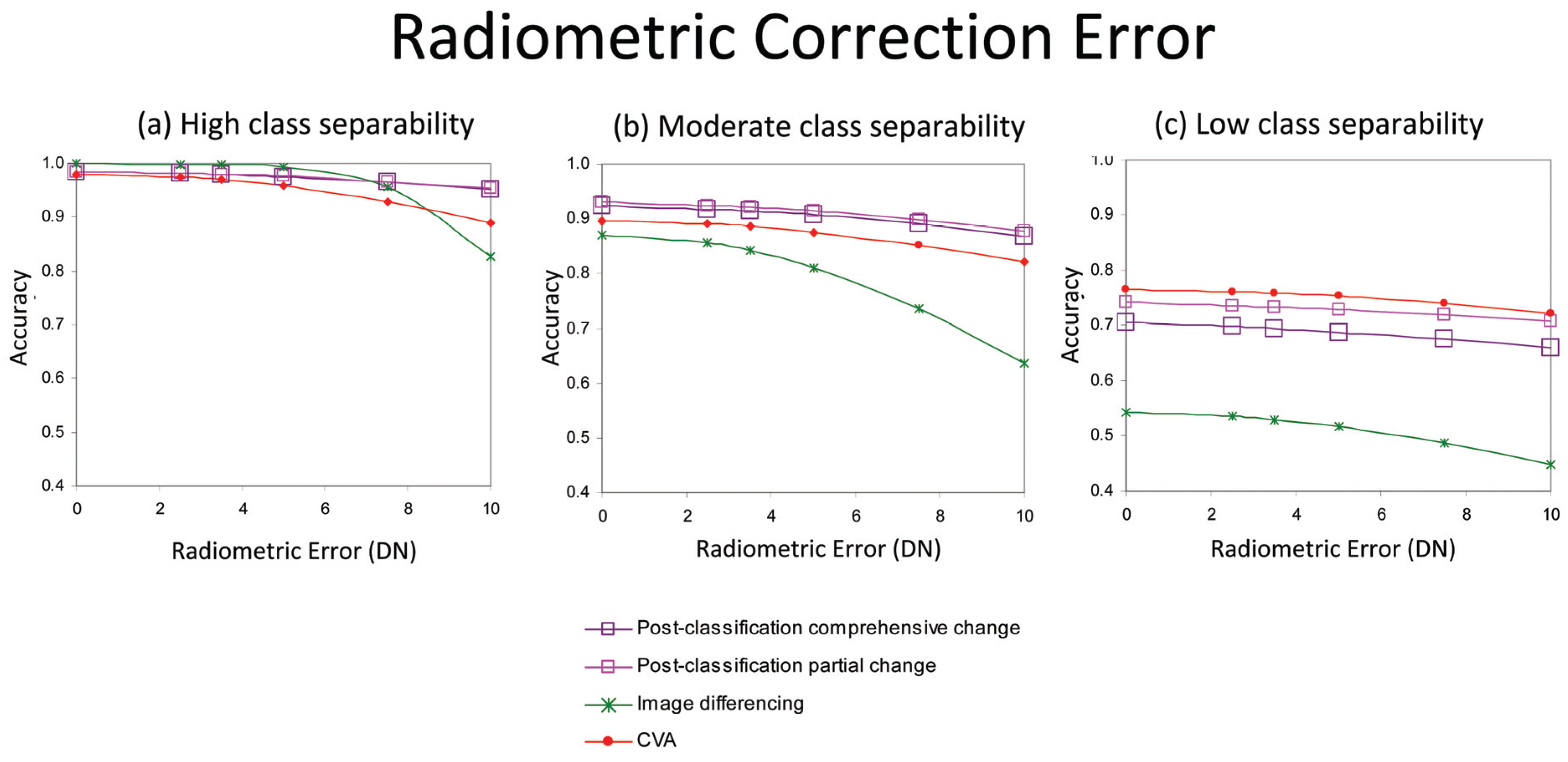
The simulated data for the radiometric normalization error experiments were developed with two bands of data, and, as with the class separability experiments, four classes for each simulated date. Three sets of sub-experiments were run, using images with high, moderate, and low class separability (Figure 7). Radiometric normalization is only necessary for the three change detection methods of image differencing, post-classification using a single set of training data, and CVA. For completeness sake, both partial and complete post-classification comparison were included, and thus Figure 7 includes a total of four methods on each graph.

Figure 7. Effect of radiometric normalization error on accuracy of change analysis methods, for simulated classes with high, moderate and low separability.

Figure 7. Effect of radiometric normalization error on accuracy of change analysis methods, for simulated classes with high, moderate and low separability.

Post-classification comparison, for both comprehensive and partial change analysis, showed the least change in accuracy as the radiometric error increased. For post-classification comparison, the comparatively large radiometric error of 10 DN reduced the accuracy by only 0.03–0.06. For relatively low class separabilities (Figure 7(c)), partial change post-classification comparison was notably more accurate than comprehensive change analysis. In other words, differentiating the various unchanged classes added notably to the overall error, unlike the moderate and high separability simulations (Figure 7(a,b)).

For classes with high separability, image differencing had the highest classification accuracy of the methods tested for radiometric errors less than 7 DN. This result was the opposite of the moderate and low separability simulated data set experiments, where image differencing was found to have the lowest accuracy for all levels of radiometric error tested. The comparatively high accuracy of image differencing for high-separability classes is supported by the separability experiments. A second notable feature of image differencing for high separability classes is that although accuracy for this method was the least affected by radiometric errors of 4 DN or less, at radiometric errors greater than 8 DN, accuracy was the most affected, dropping rapidly, to 0.8 at 10 DN. For the moderate separability simulated data set, the accuracy of image differencing was also found to decrease rapidly for radiometric errors of greater than 4 DN. For the low separability data, image differencing resulted in low accuracy, irrespective of the degree of radiometric error.

CVA behaves in very complex way throughout the three experiments. At high class separability, CVA produced the lowest accuracy for small radiometric errors. For moderate class separabilities, CVA accuracy tends to parallel the post-classification comparison accuracy results, but at a lower accuracy. Where class separability is very low, CVA was found to have the highest accuracy of any method. This result is also surprising, because post-classification comparison is often assumed to be the most accurate method [23].

In summary, the second set of normalization experiments showed the relative accuracy of the different methods is highly dependent on the interaction of radiometric normalization error and class separability. With high class separability, and low radiometric error, image differencing was found to be the most powerful method. Image differencing however, showed the most rapid decrease in accuracy, as radiometric error increased and was the least accurate for all other situations. With high class separability and large radiometric error, or moderate class separability irrespective of radiometric error, post-classification comparison gave the highest accuracy. With low class separability and low to moderate radiometric error, CVA was the most accurate method.

5.3. Band Correlation

The last set of simulated data experiment examined how the accuracy of change detection methods was affected by the correlation between image bands. As with the radiometric normalization experiments, two bands of data were created for each simulated image in the multitemporal pair. The experiment was repeated with means widely dispersed in the feature space, moderately dispersed, and clustered along the diagonal, respectively. As with the class separability experiments, all five partial and three comprehensive change methods were used.

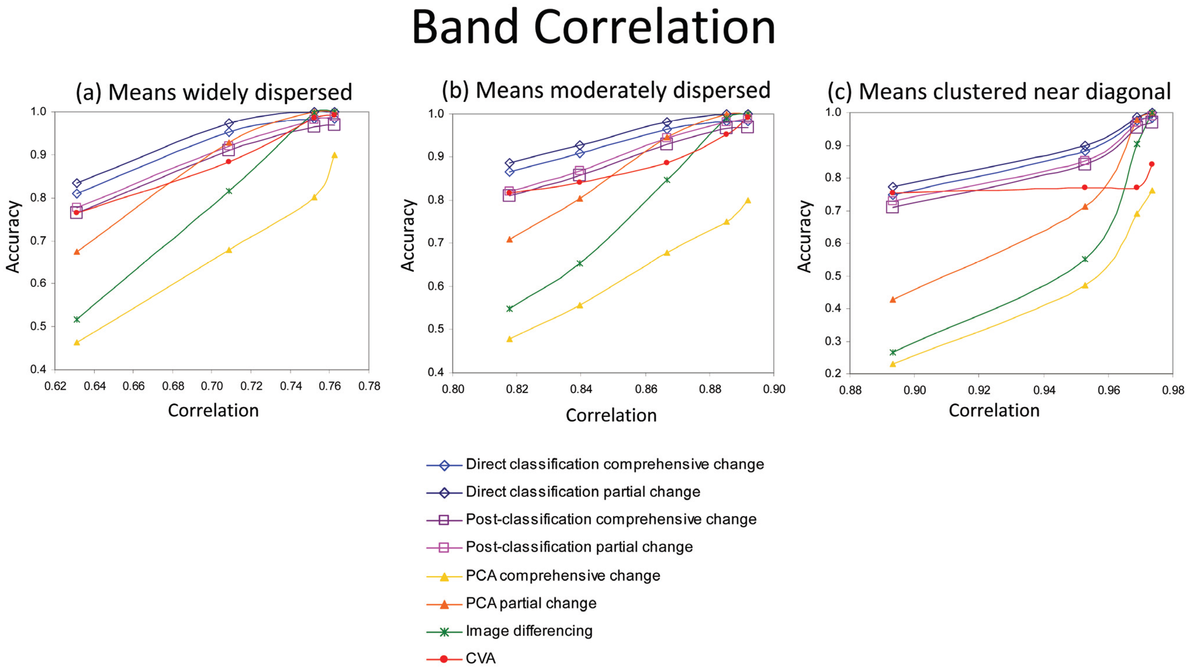
The band correlation experiments showed a general pattern of correlation and accuracy being positively associated within each individual experiment (Figure 8). However, for the data set with class means widely dispersed in the feature space, high accuracies were achieved with relatively low correlation between bands. Thus the experiments highlight that the correlation between bands is a result of two different characteristics of the data. The addition of noise to data set reduces class separability as well as the correlation between bands. Thus the pattern within each graph in Figure 8 can be understood as being driven by varying levels of noise. On the other hand, the wide distribution of the class means in the feature space away from the diagonal of the feature space reduces the correlation between the bands but also increases class separability. Thus, the differences between the three graphs are a result of class separability and its influence on class separability.

Direct classification, including both comprehensive change analysis and partial change analysis, generally produced the highest accuracy in the three experiments, especially for the data with the lowest correlation values within each experiment. For these experiments, post-classification comparison appeared to be slightly less accurate, producing results that mirrored the direct classification results, except at a lower accuracy. The accuracies obtained from the PCA comprehensive change analysis are notably different from those produced by the PCA partial change analysis. PCA comprehensive change analysis consistently had the lowest accuracy for all correlation values. On the other hand, the PCA partial change analysis showed a large improvement in accuracy with increasing correlation, especially for widely dispersed class means, where the method was similar to, or better than, the best methods. In fact, at the highest degrees of correlation, PCA partial change analysis was found to be better than post-classification comparison.

Figure 8. Effect of between band correlation on accuracy of change analysis methods, for simulated data with means widely dispersed in the spectral data space, means moderately dispersed, and means clustered near the diagonal.

Figure 8. Effect of between band correlation on accuracy of change analysis methods, for simulated data with means widely dispersed in the spectral data space, means moderately dispersed, and means clustered near the diagonal.

Image differencing also resulted in low accuracy rates for low correlation data, though not as low as PCA comprehensive change analysis. However, like PCA partial change analysis, image differencing produced one of the highest accuracies at high correlation values. Image differencing appears to be the most sensitive technique to the degree of correlation between bands, producing the greatest change in accuracy as correlation changes. In contrast, CVA is the least affected by change in the degree of correlation, especially when class means are clustered along the diagonal. Figure 8(c), for example, shows almost no change in accuracy for CVA over a wide range of correlation values. When the means of the classes were moderately and widely dispersed, and the degree of correlation was very high, CVA produced a higher accuracy than partial change post-classification comparison.

In summary, for the correlation experiments, direct classification tended to be the most accurate method, and PCA comprehensive change the least. CVA, especially when the means of the classes are clustered near the diagonal, showed the least change with degree of correlation. PCA, along with image differencing, showed the greatest sensitivity to band correlation. Although PCA for comprehensive change analysis was generally poor, PCA for partial change analysis with class means widely and moderately distributed, and relatively high degrees of correlation, was found to be one of the most accurate methods.

6. Discussion

The primary aim of this research was to investigate, using simulated data, the hypothesis that image properties have an influence on change detection accuracy. The results of these experiments suggest very strongly that this hypothesis is indeed correct. This conclusion provides an explanation for the apparent contradiction of the relative ranking of different change detection methods in previous studies, in that those studies have for the most part used just a single image data set. Our research findings imply that generalization from a single data should be carried out with caution, and preferably only to images with similar image properties. Therefore, it would be useful if in future change detection studies the authors provide as much detail as possible about the spectral properties of the images used.

The application of these results to real images is not a direct focus of this research. Nevertheless, it is useful to consider whether the image properties used in this study are commonly found in real data. The class separability experiments compared classes that ranged from a JM distance separability of 1.414 to 1.057. Thus, the experiments included class seperabilities that ranged from perfectly separable, to moderately or even poorly separated. This is a relatively conservative range of values compared to values reported in the literature. For example, in a study examining the spectral separability of burned and unburned areas in Landsat ETM+ data, J-M distances varied between less than 0.4 and 1.414 [39]. An investigation of the ability to discriminate an invasive shrub in Landsat ETM+ bands and related spectral transformations such as image ratios catalogued JM values that ranged from 0.715 to 1.230 [40]. Similarly, a study of spatial and spectral features useful in discriminating urban vegetation classes found mean JM values that varied from 0.592 to 1.113 [41].

Evaluating the realism of the radiometric offset and band correlation experiments is less straightforward. The offsets varied from 0 to 10, which at face value would appear to be a much larger range than would likely be found with reasonably well-calibrated data. Nevertheless, it is important to consider that the simulated data were designed to have a large dynamic range, exploiting the full 256 gray levels of 8-bit data. Thus the offset range modeled is not as extreme as it might appear.

Providing guidance to practitioners regarding the optimal methods to use for different images is beyond the scope of this work, and will be the subject of future research. However, some general inferences can be drawn from these results. Firstly, as might be expected, if classes are highly separable, the choice of change detection method can safely be based on criteria other than the relatively accuracy of the different methods, since all methods are likely to do well. Likewise, for highly separable classes, error in the radiometric normalization produces relatively little added error to the change detection.

In comparison, for moderately and poorly separated classes, the change detection method is important, and image differencing in particular should be avoided. Generally, post-classification comparison is a robust method, but our work also suggests that CVA can be an effective tool in such circumstances. For moderately-well separated classes, obtaining the highest possible accuracy for radiometric is crucial.

The band correlation experiments are more difficult to generalize from, primarily because a low degree of inter-band correlation can indicate a low separability between classes due to uncorrelated noise, or due to classes that are spectrally very different. Thus, correlation cannot simply be related to class separabilty.

7. Conclusions

The results from the three experiments using simulated data showed that no single change detection method consistently produced the highest accuracy as image spectral properties varied. Thus these experiments appear to confirm the hypothesis that previous change detection analysis comparisons do not help elucidate the general strength of each method, unless the spectral properties of the images used can be placed in a larger context.

Although the results are complex, some general patterns emerge. In most cases, direct classification and post-classification comparison were the least sensitive to changes in the image properties of class separability, radiometric normalization error and band correlation. Furthermore, these methods generally produced the highest accuracy, or were amongst those with a high accuracy.

PCA change analysis produced very different results in different circumstances, as might be expected for a method that is inherently scene-specific. In particular, the number of components used is very important, as is the choice between partial and comprehensive change analysis. The use of four principal components consistently resulted in substantial decreased classification accuracy relative to using six components, or classification using the original six bands.

The accuracy of image differencing also varied greatly in the experiments. For example, in order to achieve high levels of accuracy with image differencing, low errors in radiometric normalization and high class separabilities are required. Of the three methods that require radiometric normalization, image differencing was the method most affected by radiometric error, relative to change vector and classification methods, for classes that have moderate and low separability. For classes that are highly separable, image differencing was relatively unaffected by radiometric normalization error.

CVA accuracies also varied greatly, although this method tended to be the least affected by changes in the degree of band correlation in situations where the class means were moderately dispersed, or clustered near the diagonal. CVA was also found to be the most accurate method for classes with low separability and all but the largest radiometric errors.

For all change detection methods, the classification accuracy increased as simulated band correlation increased, and direct classification methods consistently had the highest accuracy, while PCA generally had the lowest accuracy.