Normalizing and Converting Image DC Data Using Scatter Plot Matching

Abstract

Remote sensing image data from sources such as Landsat or airborne multispectral digital cameras are typically in the form of digital count (DC) values. To compare images acquired by the same sensor system on different dates, or images acquired by different sensor systems, it is necessary to correct for differences in the DC values due to sensor characteristics (gain and offset), illumination of the surface (a function of sun angle), and atmospheric clarity. A method is described for normalizing one image to another, or converting image DC values to surface reflectance. This method is based on the identification of pseudo-invariant features (bare soil line and full canopy point) in the scatter plot of red and near-infrared image pixel values. The method, called “scatter plot matching” (SPM), is demonstrated by normalizing a Landsat-7 ETM+ image to a Landsat-5 TM image, and by converting the pixel DC values in a Landsat-5 TM image to values of surface reflectance. While SPM has some limitations, it represents a simple, straight-forward method for calibrating remote sensing image data.

1. Introduction

The image data produced by remote sensing systems such as Landsat TM or airborne digital cameras are typically in the form of digital count (DC) values. DC values are related to the reflectance of the observed surface but are affected by other factors, including sensor characteristics (gain and offset), illumination of the surface (a function of sun angle), and atmospheric clarity. To compare images acquired by the same sensor system on different dates, or images acquired by different sensor systems, it is necessary to correct for differences in the DC values present in the images as a result of differences in the previously mentioned factors. This can be accomplished either by absolute radiometric correction or relative calibration [1]. In absolute radiometric correction, DC values are converted to values of surface reflectance. In relative calibration, the DC values of one image are normalized to those of another image to provide a relative correction for sensor, illumination, and atmospheric differences.

For satellite imagery, correction of DC values for sensor characteristics and sun angle is relatively straight-forward by calculating corresponding values of exoatmospheric reflectance based on known sensor gain and offset parameters and the time of day and day of year [2]. A similar procedure can be used to calculate at-sensor reflectance for aircraft imagery. The remaining problem is to correct these values for the effects of the atmosphere along the observing path. Numerous approaches for atmospheric correction of satellite and aircraft imagery have been described and compared [1,3,4,5,6,7]. These approaches can be separated into two general groups: physically based correction methods, and image-based correction methods. Physically based correction methods use some form of radiative transfer model (RTM) to explicitly compute the effects of atmospheric scattering and absorption on the electromagnetic signal as it passes from the surface to the sensor. These methods can be highly accurate, but they require information in addition to the image data that describes the optical characteristics of the atmosphere (as a function of its water vapor and aerosol content) along the observing path. Image-based methods utilize solely the information in the remote sensing image. A variety of image-based methods have been described. For relatively low-altitude aircraft imagery, DC values can be converted based on the known reflectance of specially fabricated targets placed on the ground so as to be visible within the acquired imagery. Disadvantages of this approach are that a special effort must be made to place the targets in the area to be imaged, and that it is not effective for high-altitude aircraft or satellite observations due to the relatively small size of the targets. Large natural or man-made objects with relatively uniform reflectance characteristics, such as lakes or airport runways, have been used to correct aircraft and satellite image data. A problem with these “pseudo-invariant objects” is that their reflectance tends to change over time due to the effects of weather [7]. In another image-based method, DC values extracted for a clear lake present in the image were used to implicitly estimate atmospheric transmittance and scattering using an RTM [8]. A related method, “dark object subtraction” (DOS), uses the darkest object in the image (assumed to be in deep shadow) to estimate the atmospheric scattering component of the signal received by the sensor [9,10]. The success of these methods rests on finding clear lakes or objects with apparent reflectances of around 1% in the image.

Several image-based methods have been developed that make use of “pseudo-invariant features” (PIFs) to normalize one remote sensing image to another. Working with Landsat, Schott et al. [11] used an infrared-red ratio image derived from TM Bands 4 and 3 to develop a PIF mask to identify and collect DC data for man-made features in images acquired on different dates. The means and variances of the distributions of PIF DC values are used to evaluate a linear regression for transforming DC values in one image to be comparable to those in the other image. Hall et al. [12] described a method that can normalize one image to another using information derived from the two-dimensional scatter plot of Kauth-Thomas greenness and brightness [13]. In this approach, “radiometric control sets” (RCSs) of pixel DC values corresponding to the darkest (such as deep reservoirs) and brightest (such as concrete or rock outcrops) non-vegetated portions of the scatter plot are used to evaluate a linear regression for transforming DC values in one image to be comparable to those in the other image. The RCSs are associated with PIFs in the scatter plot and may not include the same pixels from image to image. For both of these approaches, it is assumed that bright and dark features are present in the imagery, and the reflectance characteristics of these PIFs are invariant over time.

Remote sensing imagery of agricultural regions is dominated by vegetation and soil, and may be devoid of the kinds of bright and dark features (deep lakes, rock outcrops, or large man-made objects) used in the previously described methods. In this study, we developed a procedure to convert image DC values in the red and near-infrared (NIR) spectral bands into corresponding values of surface reflectance based on PIFs associated with vegetation and soil. This method can also normalize the red and NIR image bands in one image to another image. The method automatically accounts for the effects of sensor characteristics, surface illumination, and certain aspects of atmospheric absorption and scattering. Application of the method is illustrated using Landsat imagery, and a test of its accuracy using independent data is provided. Finally, potential limitations of the method are discussed.

2. Theory

2.1. Red-NIR Scatter Plot

When the DC values in the NIR spectral band are plotted versus the corresponding DC values in the red spectral band for pixels comprising a cloud-free multispectral image of an agricultural region, a characteristic distribution of points is produced [14,15]. An example is presented in Figure 1A. This roughly triangular distribution of points results from the reflectance characteristics of vegetation and soil, and the mixing of these characteristics within image pixels. Image pixels containing only bare soil lie along the diagonal “base” of the triangle, forming a line commonly called the “bare soil line”. This line is shown in Figure 1B, which provides a diagrammatic representation of the distribution of points in Figure 1A. Point a represents the brightest soil in the satellite image, while point b represents the darkest soil in the satellite image. For a single soil type, point a might correspond to pixels containing only dry soil, while point b might correspond to pixels containing only wet soil. Points along the soil line between a and b would correspond to pixels with intermediate levels of soil wetness, or pixels with varying mixtures of wet and dry soil. Points in the distribution above and to the left of the bare soil line represent pixels containing living vegetation. Since living vegetation strongly absorbs light in the red band and strongly reflects light in the NIR band, increasing the amount of vegetation in a pixel decreases the brightness of the pixel in the red band and increases the brightness of the pixel in the NIR band. As vegetation cover increases, the effects of background soil brightness decreases. At full canopy, the vegetation completely obscures the soil surface, a situation represented by a single point (point c) in Figure 1B. The leaves of many plants absorb only a small fraction of light in the NIR, and reflect and transmit the remainder in roughly equal proportions [16]. As a result, the DC value in the NIR spectral band for a pixel with full canopy can continue to increase as the density of the leaf canopy increases, due to the upward scattering and transmission of light by leaves lower in the plant canopy. Thus, it is possible to observe a “spike” of points in the scatter plot extending above the point normally corresponding to full canopy. This feature appears in Figure 1A, and is represented diagrammatically in Figure 1B by the line segment between points c and d.

Figure 1. Red-NIR scatter plot of pixel DC values for a portion of a cloud-free Landsat-5 image of an agricultural region. (A) Actual distribution of DC values. (B) Diagrammatic representation of features of the scatter plot of DC values.

Figure 1. Red-NIR scatter plot of pixel DC values for a portion of a cloud-free Landsat-5 image of an agricultural region. (A) Actual distribution of DC values. (B) Diagrammatic representation of features of the scatter plot of DC values.

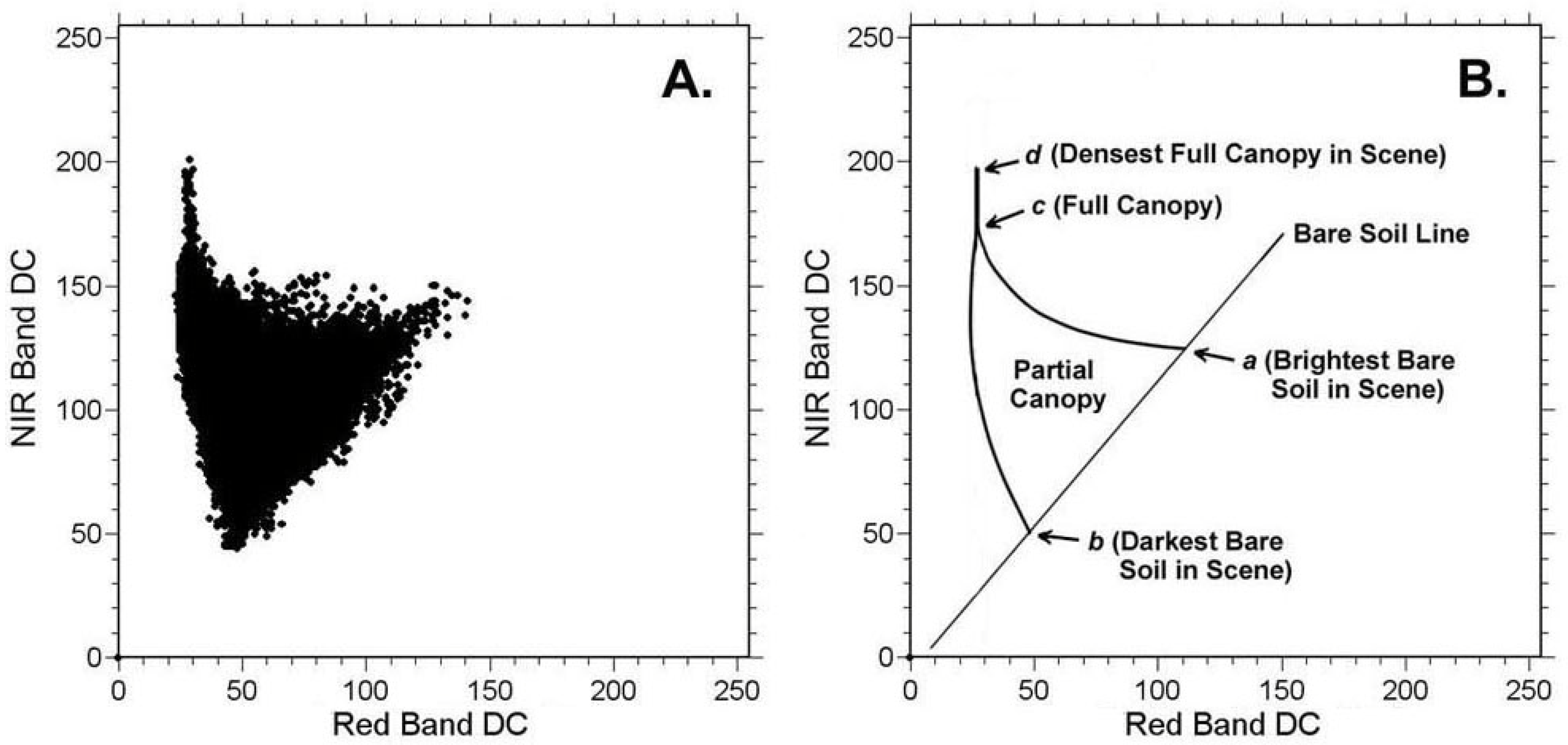
Two characteristic features of the distribution of DC values in Figure 1 are the bare soil line and the full canopy point. While the specific DC values associated with each may be different between images, they will almost always be identifiable in the red-NIR scatter plot for images containing vegetation and soil. Thus, the bare soil line (BSL) and full canopy point (FCP) represent PIFs within the red-NIR scatter plot. As we will show in the following sections, these PIFs can be used to normalize one image to another and convert image DC values to surface reflectance.

2.2. Transforming Images Using BSL and FCP PIFs

For many remote sensing imaging systems, such as Landsat TM, image DC values are a linear function of the radiance reaching the sensor [11,18],

DC_i,j = g_j R_i + o_j

(1)

where DC_i,j is the DC for pixel i and band j, R_i is the radiance observed for pixel i, and g_j and o_j are the sensor gain and offset for band j. Similarly, the radiance reaching the sensor is, to a first-order approximation, a linear function of surface reflectance [11],

R_i, = K_1,j r_i + K_2,j

(2)

where r_i is the reflectance of the surface for pixel i and K_1,j and K_2,j are parameters related to surface irradiance and atmospheric clarity. The value of K_1,j should be proportional to surface irradiance and atmospheric transmissivity. The value of K_2,j should be proportional to optical path radiance. Since atmospheric transmissivity and path radiance can vary according to wavelength, the values of K_1,j and K_2,j may be band-specific.

The consequence of Equations 1 and 2 is that changes in sensor characteristics, surface irradiance, and atmospheric clarity between image acquisitions should result in linear scalings and translations of the distribution of DC values shown in Figure 1A within the red-NIR scatter plot space. However, these changes do not alter the basic relationship between the BSL and FCP PIFs within the DC distribution for an image. Thus, we have determined that, if one knows the equation of the BSL and the red and NIR values for the FCP for two images, this information can be used to normalize the red and NIR bands of one image to those of the other image. Furthermore, if the equation of the BSL and the red and NIR values for the FCP can be expressed in terms of surface reflectance, this information can be used to convert the red and NIR bands of an image from DC to surface reflectance.

The equations needed to carry out these transformations are as follows,

Y_i,NIR = DC_i,NIR β₁ + β₂

(3)

X_i,red = DC_i,red β₃ + β₄

(4)

in which Y_i,NIR and X_i,red are the transformed values of DC_i,NIR and DC_i,red, respectively, for pixel i in the red and NIR image bands. The parameters β₁–β₄ are evaluated from two sets of values for the slope and intercept of the BSL and the coordinates of the FCP. One set of these values comes from the scatter plot for the image to be transformed, which we call the “target” image. The second set of values is called the “reference” set, and provides the basis for the transformation. These reference values may come from the scatter plot for another image (the “reference” image). If the pixel values for this reference image are in the form of DCs, then Y_i,NIR and X_i,red will also be in the form of DCs, and the target image will be normalized to the reference image. If the pixel values for the reference image are in the form of reflectance, then Y_i,NIR and X_i,red will be in the form of reflectance, and the target image will be converted from DC to reflectance. Alternately, the reference set of values for the slope and intercept of the BSL and the coordinates of the FCP could be determined from ground-based field measurements instead of from a reference image.

The parameters in Equations 3 and 4 are evaluated as follows,

$${\beta }_1=\frac{y_{fc,ref}-\left(a_{1,ref}{x}_{fc,ref}+a_{0,ref}\right)}{y_{fc,tar}-\left(a_{1,tar}{x}_{fc,tar}+a_{0,tar}\right)}$$

(5)

β₂ = y_fc,ref – y_fc,tar β₁

(6)

β₃ = (a_1,tar β₁) / a_1,ref

(7)

β₄ = x_fc,ref – x_fc,tar β₃

(8)

In these equations, a_1,ref and a_0,ref are the reference values for the slope and intercept, respectively, of the BSL, while x_fc,ref and y_fc,ref are the reference values for the coordinates of the FCP for the red and NIR spectral bands, respectively. Similarly, a_1,tar and a_0,tar are the target image values for the slope and intercept, respectively, of the BSL, while x_fc,tar and y_fc,tar are the target image values for the coordinates of the FCP for the red and NIR spectral bands, respectively.

Once the reference and target values for the slope and intercept of the BSL and the coordinates of the FCP have been determined, the pixel values in the target image can be normalized or converted to surface reflectance using Equations 3 and 4. Since this procedure transforms the features of one scatter plot to match the corresponding features of another, we have called it “scatter plot matching” (SPM).

3. Materials and Methods

3.1. Demonstration of Image Normalization

To demonstrate normalizing one image to another using the SPM method, two Landsat images were obtained. One image was acquired on 17 August 2009 from the ETM+ sensor aboard Landsat-7 for WRS Path 30, Row 36. The other image was acquired eight days later (25 August 2009) from the TM sensor aboard Landsat-5 for the same location. A 790 × 1,575-pixel section was extracted from the central portion of the red and NIR image bands for each acquisition. This section was chosen to avoid most of the scan line problems present in current ETM+ images [18]. The TM image section was cloud-free, while the ETM+ image section contained a few scattered patches of small cumulus clouds, along with their shadows. The TM image was arbitrarily chosen to be the reference image, while the ETM+ image was chosen to be the target image. Red-NIR scatter plots were constructed for the reference and target image sections, and the BSL and FCP were identified in each scatter plot by visual inspection [19]. The slope and intercept of the BSL were determined for each scatter plot, along with the DC coordinates of the FCP. These values were used to evaluate parameters β₁–β₄ using Equations 5–8. The parameter values were then applied to normalizing each pixel DC value in the red and NIR image bands of the target image section using Equations 3 and 4, resulting in the generation of a normalized target image section. The red-NIR scatter plot for the normalized target image was compared with that from the reference image to show the effects of normalization.

3.2. Conversion of an Image to Reflectance Based on Field Observations

As stated earlier, if the equation of the BSL and the red and NIR values for the FCP can be expressed in terms of surface reflectance, this information can be used to convert the red and NIR bands of an image from DC to surface reflectance. Field data were collected to evaluate the BSL and FCP in terms of surface reflectance from ground-based measurements. The resulting slope and intercept of the BSL and the red-NIR values for the FCP were used to compute the values of β₁–β₄, which in turn were used to convert Landsat TM images from DC to surface reflectance using Equations 3 and 4.

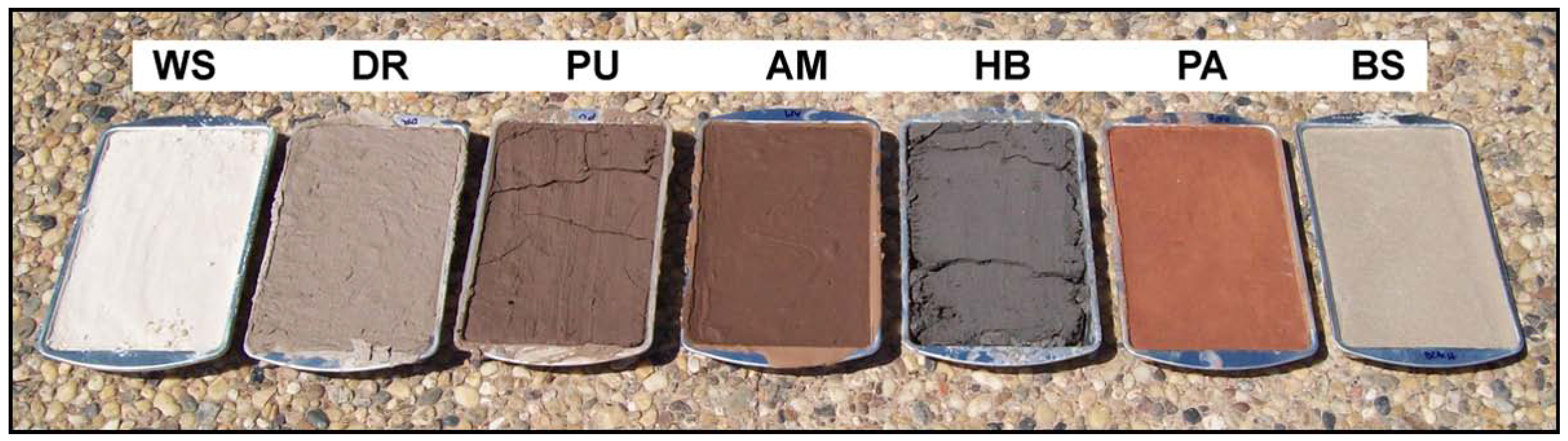
To evaluate the BSL, measurements were made on seven soils collected from different locations. These soils were collected from the upper 15 cm of the profile, and exhibited considerable variation in their physical characteristics (Table 1). While the beach sand and gypsum sand are technically not soils, for the sake of simplicity they will be referred to as “soils” in this study. To prepare the soils for measuring their reflectance, a sample of each was saturated with water in a bucket. The sample was then placed in a 27 × 18 × 3.5-cm aluminum tray and the surface was scraped smooth by running a wooden board with a straight edge along the top of the tray (Figure 2). Reflectance measurements of the soil surface were begun immediately after scraping. Reflectance measurements were made outdoors using a GER-1500 portable field spectroradiometer (Spectra Vista Corp., Poughkeepsie, NY, USA) under clear sky conditions. Measurements with the GER-1500 were calibrated using frequent measurements on a 7.5 cm-diameter circular Spectralon target (Labsphere, Inc., North Sutton, NH, USA). Frequent reflectance measurements were made on the soil as it dried. The tray with the soil was returned to the lab and allowed to dry additionally for approximately one week until it appeared to be in an air-dry state. It was then taken outdoors for additional reflectance measurements. These measurements were repeated on the following day to verify that the soil reflectance was not changing. The tray with the soil was then placed in a ventilated drying oven at 100 °C for approximately one week until it appeared to be in an oven-dry state. It was then taken outdoors for additional reflectance measurements. As before, these measurements were repeated on the following day to verify that the soil reflectance was not changing. In all, the reflectance measurements made on a soil spanned the range of soil wetness from saturated to oven-dry.

Table 1. Characteristics of the seven soils used in the study.

Symbol	Soil Name	Location Found	Soil Texture			Soil Type	Dry Soil Color
			% sand	% silt	% clay		general	Munsell
AM	Amarillo	Lubbock Co., TX	64	16	20	sandy loam	reddish brown	7.5YR 4/4
HB	Houston Black	Bell Co., TX	10	36	54	clay	black	2.5Y 4/1
BS	beach sand	South Padre Is., TX	89	2	9	sand	tan	10YR 7/3
DR	Drake	Hale Co., TX	74	6	20	sandy loam	light gray	10YR 6/2
PU	Pullman	Hale Co., TX	48	20	32	sandy clay loam	dark brown	7.5YR 4/3
PA	Paducah	Fisher Co., TX	62	18	20	sandy loam	red	2.5YR 5/6
WS	gypsum sand	White Sands Nat. Mon., NM	87	2	11	sand	white	5Y 8/1

Note: Except for the beach and gypsum sands, the soil name refers to its soil series.

Table 1. Characteristics of the seven soils used in the study.

Symbol	Soil Name	Location Found	Soil Texture			Soil Type	Dry Soil Color
			% sand	% silt	% clay		general	Munsell
AM	Amarillo	Lubbock Co., TX	64	16	20	sandy loam	reddish brown	7.5YR 4/4
HB	Houston Black	Bell Co., TX	10	36	54	clay	black	2.5Y 4/1
BS	beach sand	South Padre Is., TX	89	2	9	sand	tan	10YR 7/3
DR	Drake	Hale Co., TX	74	6	20	sandy loam	light gray	10YR 6/2
PU	Pullman	Hale Co., TX	48	20	32	sandy clay loam	dark brown	7.5YR 4/3
PA	Paducah	Fisher Co., TX	62	18	20	sandy loam	red	2.5YR 5/6
WS	gypsum sand	White Sands Nat. Mon., NM	87	2	11	sand	white	5Y 8/1

Note: Except for the beach and gypsum sands, the soil name refers to its soil series.

The GER-1500 produced reflectance spectra over the range 290 to 1130 nm at nominally 2-nm increments. Values within the Landsat TM red spectral band (630–690 nm) and NIR spectral band (760–900 nm) were averaged to produce “red” and “ NIR” soil reflectance values, respectively. Values of NIR soil reflectance were plotted versus corresponding values of red soil reflectance, and this distribution of points was fit using simple linear regression to produce an equation for the BSL.

Figure 2. Trays holding the seven soils for reflectance measurements.

Figure 2. Trays holding the seven soils for reflectance measurements.

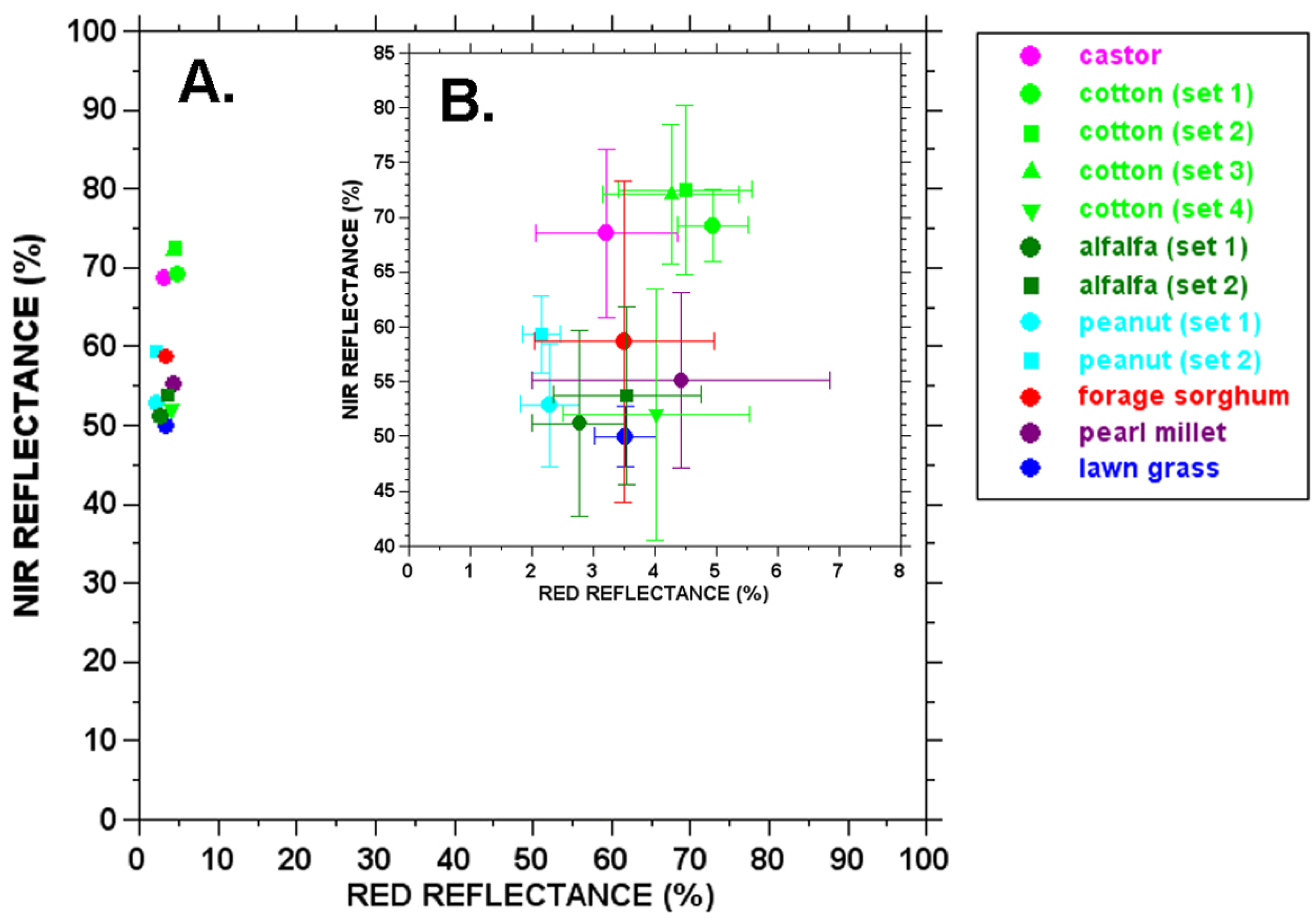
To evaluate the FCP, reflectance measurements were made on the leaf canopies of seven plant species commonly found in the region (Table 2). In some cases, measurements were made at more than one site. Measurements were made on canopies with full ground cover. Measurements were made using the GER-1500 at a height of approximately 1 m above the top of the canopy. The measurements were calibrated in the same manner as described for the soil reflectance measurements. From 7 to 12 individual spectra were measured at each site, and “red” and “NIR” reflectance values were determined for the Landsat TM red and NIR spectral bands as previously described. The mean and standard deviation for the red and NIR canopy reflectance measurements were calculated from these data for each site. Values of NIR canopy reflectance were plotted versus corresponding values of red canopy reflectance and analyzed to produce the red and NIR coordinates of the FCP.

Table 2. The seven plant species used in the study for determining canopy reflectance.

Data set		Location	Date	Site	No. of Spectra Measured	Canopy Height (cm)
1	pearl millet	Hale Co., TX	August 2008	farmer’s field	10	80
2	alfalfa (set 1)	Hale Co., TX	August 2008	farmer’s field	10	45
3	alfalfa (set 2)	Hale Co., TX	July 2006	farmer’s field	12	45
4	peanut (set 1)	Lubbock Co., TX	August 2008	research plot	12	25
5	peanut (set 2)	Lubbock Co., TX	August 2008	research plot	9	30
6	cotton (set 1)	Lubbock Co., TX	August 2008	research plot	11	80
7	cotton (set 2)	Lubbock Co., TX	August 2008	research plot	7	100
8	cotton (set 3)	Lubbock Co., TX	August 2008	research plot	7	100
9	cotton (set 4)	Hale Co., TX	July 2006	farmer’s field	12	60
10	castor	Lubbock Co., TX	August 2008	research plot	11	120
11	forage sorghum	Hale Co., TX	July 2006	farmer’s field	8	200
12	lawn grass	Lubbock Co., TX	August 2008	research plot	8	3

Scientific names: pearl millet Pennisetum glaucum (L.) R. Br.; alfalfa Medicago sativa (L.); peanut Arachis hypogaea (L.); cotton Gossypium hirsutum (L.); castor Ricinus communis (L.); forage sorghum Sorghum bicolor (L.) Moench; lawn grass Bouteloua dactyloides (Nutt.) J.T. Columbus.

Table 2. The seven plant species used in the study for determining canopy reflectance.

Data set		Location	Date	Site	No. of Spectra Measured	Canopy Height (cm)
1	pearl millet	Hale Co., TX	August 2008	farmer’s field	10	80
2	alfalfa (set 1)	Hale Co., TX	August 2008	farmer’s field	10	45
3	alfalfa (set 2)	Hale Co., TX	July 2006	farmer’s field	12	45
4	peanut (set 1)	Lubbock Co., TX	August 2008	research plot	12	25
5	peanut (set 2)	Lubbock Co., TX	August 2008	research plot	9	30
6	cotton (set 1)	Lubbock Co., TX	August 2008	research plot	11	80
7	cotton (set 2)	Lubbock Co., TX	August 2008	research plot	7	100
8	cotton (set 3)	Lubbock Co., TX	August 2008	research plot	7	100
9	cotton (set 4)	Hale Co., TX	July 2006	farmer’s field	12	60
10	castor	Lubbock Co., TX	August 2008	research plot	11	120
11	forage sorghum	Hale Co., TX	July 2006	farmer’s field	8	200
12	lawn grass	Lubbock Co., TX	August 2008	research plot	8	3

Scientific names: pearl millet Pennisetum glaucum (L.) R. Br.; alfalfa Medicago sativa (L.); peanut Arachis hypogaea (L.); cotton Gossypium hirsutum (L.); castor Ricinus communis (L.); forage sorghum Sorghum bicolor (L.) Moench; lawn grass Bouteloua dactyloides (Nutt.) J.T. Columbus.

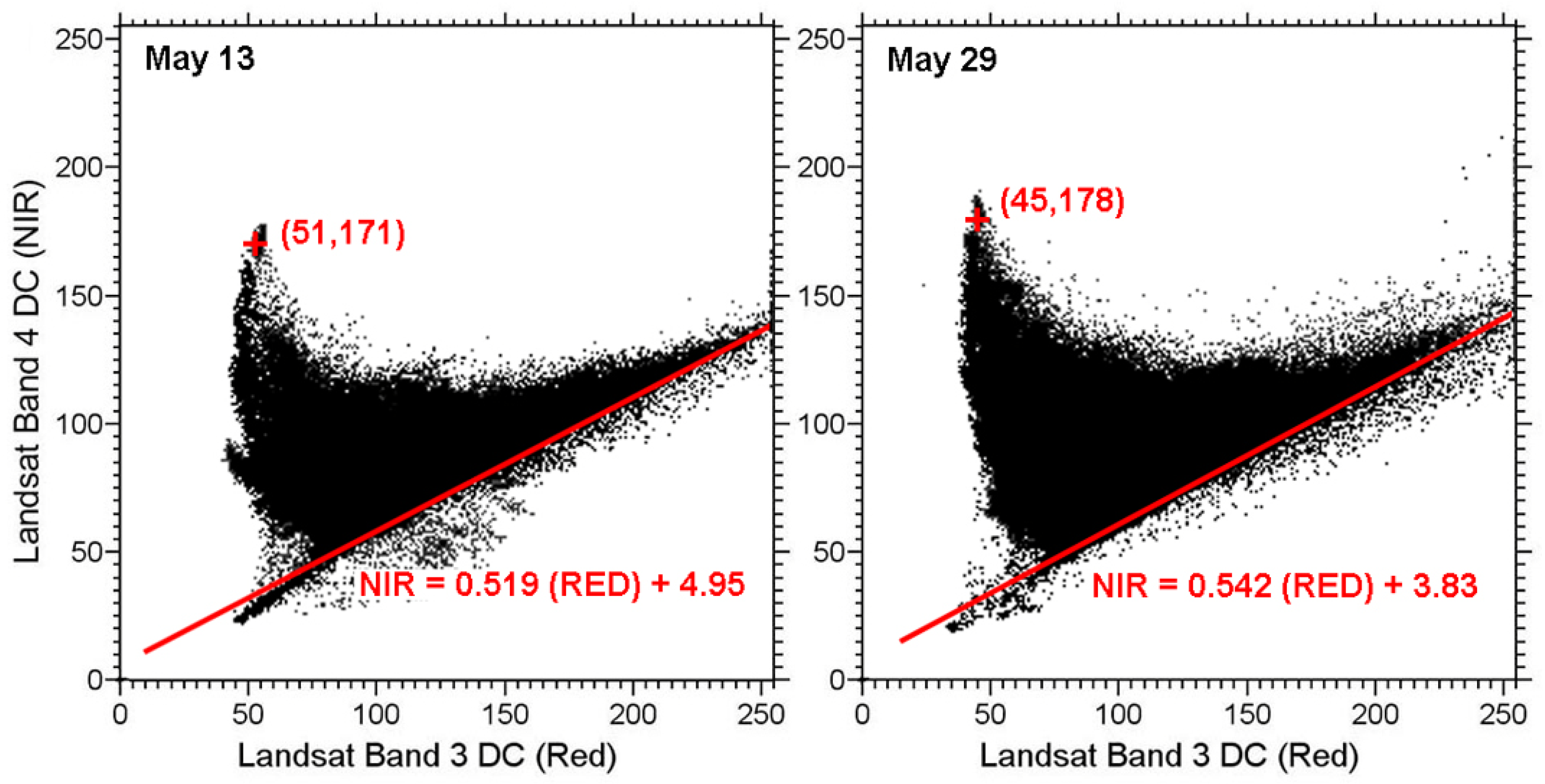
Two Landsat-5 TM images (13 May and 29 May 2009) were selected for conversion to surface reflectance. The acquisition on 13 May was for WRS Path 30, Row 37, while the acquisition on 29 May was for WRS Path 30, Row 36. These images were selected because they contained sites for which ground-based measurements of surface reflectance were made for validating the image conversion (described later in this section). The red-NIR scatter plot for each image was constructed and the BSL and FCP were identified in each scatter plot by visual inspection, as in the case of image normalization described previously. Each TM image was considered a target image and was converted from DCs to surface reflectance using Equations 3 and 4. To evaluate the parameters β₁–β₄, “target” values of the slope and intercept of the BSL and coordinates of the FCP were obtained from the scatter plot for each image, while “reference” values of the slope and intercept of the BSL and coordinates of the FCP came from the analysis of the ground-based reflectance measurements of soil and leaf canopy described earlier in this section.

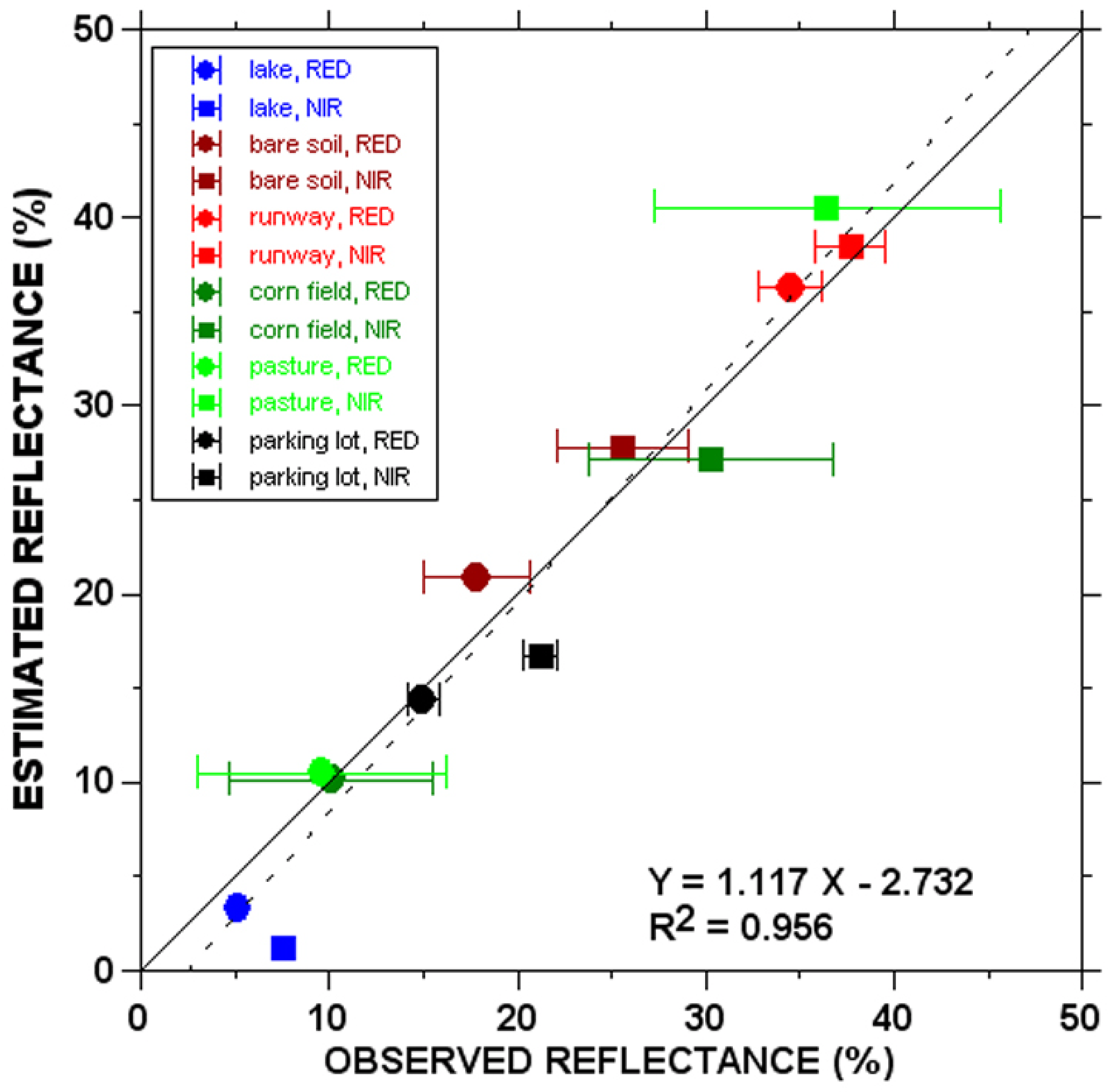
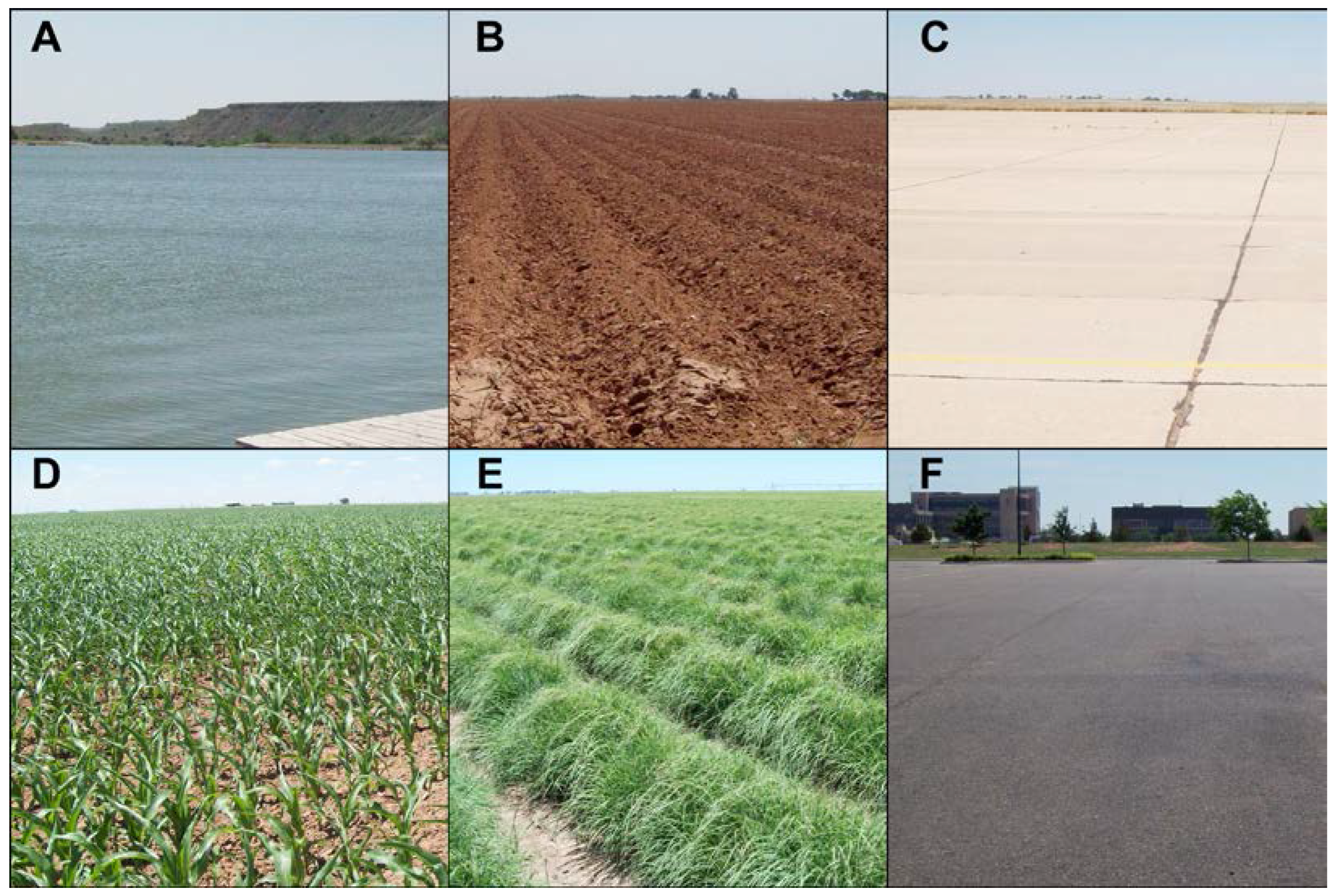
To validate the conversion of the images to surface reflectance and provide an assessment of the general accuracy of the procedure, ground-based measurements of surface reflectance were obtained for six sites contained within the two images. These sites are shown in Figure 3 and summarized in Table 3. At each site, surface reflectance was measured using the GER-1500 within 1 hour of the Landsat-5 overpass time. Measurements were calibrated using the Spectralon target as previously described. The mean and standard deviation for the red and NIR surface reflectance measurements were calculated for each site. Sets of pixels corresponding to the six ground sites were identified in the converted Landsat images and their values were extracted. The pixel values in each set were averaged to produce values corresponding to the ground-based measurements of surface reflectance. Linear regression analysis was then used to compare the surface reflectance values from the two sources.

Figure 3. The six ground sites used to validate the image conversion procedure. (A) Lake. (B) Bare soil field. (C) Runway. (D) Corn field. (E) Pasture. (F) Parking lot.

Figure 3. The six ground sites used to validate the image conversion procedure. (A) Lake. (B) Bare soil field. (C) Runway. (D) Corn field. (E) Pasture. (F) Parking lot.

Table 3. The six ground sites used to validate the image conversion procedure.

Site		Location	Date	No. of Spectra Measured
A	Lake Ransom Canyon	Lubbock Co., TX	13 May	8
B	Bare soil field	Lubbock Co., TX	13 May	8
C	Reese Airbase runway	Lubbock Co., TX	13 May	11
D	Corn field (30% GC)	Floyd Co., TX	29 May	24
E	Pasture (60% GC)	Floyd Co., TX	29 May	48
F	Texas Tech parking lot	Lubbock Co., TX	13 May	29

Table 3. The six ground sites used to validate the image conversion procedure.

Site		Location	Date	No. of Spectra Measured
A	Lake Ransom Canyon	Lubbock Co., TX	13 May	8
B	Bare soil field	Lubbock Co., TX	13 May	8
C	Reese Airbase runway	Lubbock Co., TX	13 May	11
D	Corn field (30% GC)	Floyd Co., TX	29 May	24
E	Pasture (60% GC)	Floyd Co., TX	29 May	48
F	Texas Tech parking lot	Lubbock Co., TX	13 May	29

4. Results and Discussion

4.1. Image Normalization

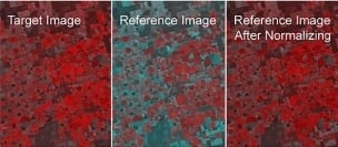
Figure 4A,B show the reference and target image sections, respectively, used in this normalization example presented as false-color composites with the NIR band displayed in the red channel and the red band displayed in the green and blue channels. There is obviously a big difference in the appearance of these two images. This difference can be explained by referring to the NIR-red scatter plots constructed for the two images (Figure 5A,B). While the pixel distributions for both images display the characteristic shape (as in Figure 1A), there are substantial differences between the equations of the BSL and the coordinates of the FCP between the two scatter plots.

Figure 4C shows the target image section after application of the normalization procedure. Its appearance is now similar to the reference image in Figure 4A. The scatter plot for the normalized image section is presented in Figure 5C, and it can be seen that the distribution of the points in it has been transformed to resemble the distribution for the reference image. The blank horizontal lines in the distribution of points in the normalized scatter plot are a computational artifact. They result from multiplying target image DC values in Equation 3 or Equation 4 by a value of β greater than 1 (in this example, β₁ = 1.16). In this situation, the resulting distribution of DC values will be expanded along the appropriate axis in the scatter plot (in this example, the NIR axis) but will not be continuous, having regular “skips” at certain values.

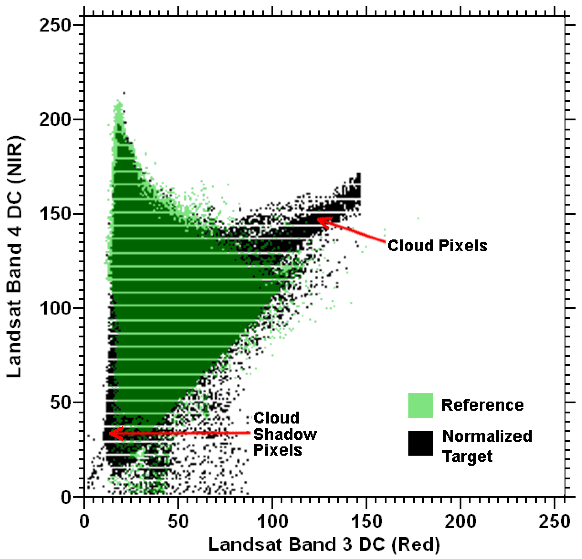
Figure 6 shows the scatter plot for the normalized target image overlaid with the scatter plot for the reference image. Following normalization, there is a good match between the distributions of points in the two scatter plots. The two main groups of points in the normalized image scatter plot for which there are not matching points in the reference image scatter plot correspond to pixels in the target image with clouds or cloud shadows (recall that the reference image was cloud-free).

4.2. Image Conversion

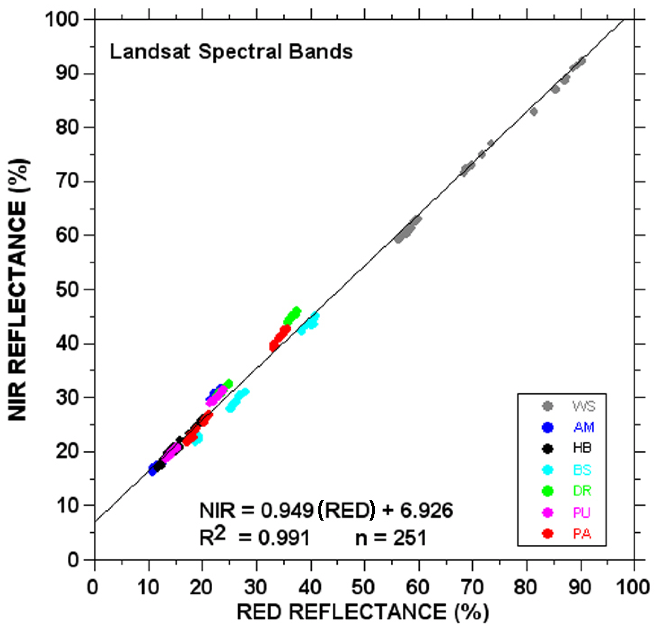
Ground-based measurements of soil reflectance in the NIR spectral band are plotted versus corresponding values in the red spectral band in Figure 7 for the seven soils used in this study (Table 1). A single, straight regression line with the equation NIR = 0.949(Red) + 6.926 with an R² of 0.991 appeared to be a reasonable fit the entire data set, with no individual observation deviating from the line by more than 3% reflectance. A few of the soils, like the beach sand and the Drake soil, appear to exhibit consistent deviations from the regression line but, again, these deviations are minor. The slope and intercept of this line are similar to values reported by other researchers. Jackson et al. [20] reported a soil line with the equation NIR = 1.18(Red) + 9.1 for an Avondale loam measured with an Exotech spectroradiometer. Analysis of reflectance values for 20 soils yielded a soil line with the equation NIR = 1.17(Red) + 4.2 [21].

Figure 4. False-color composite representations of the image sections used in the normalization example. (A) Reference image. (B) Target image before normalization. (C) Target image after normalization.

Figure 4. False-color composite representations of the image sections used in the normalization example. (A) Reference image. (B) Target image before normalization. (C) Target image after normalization.

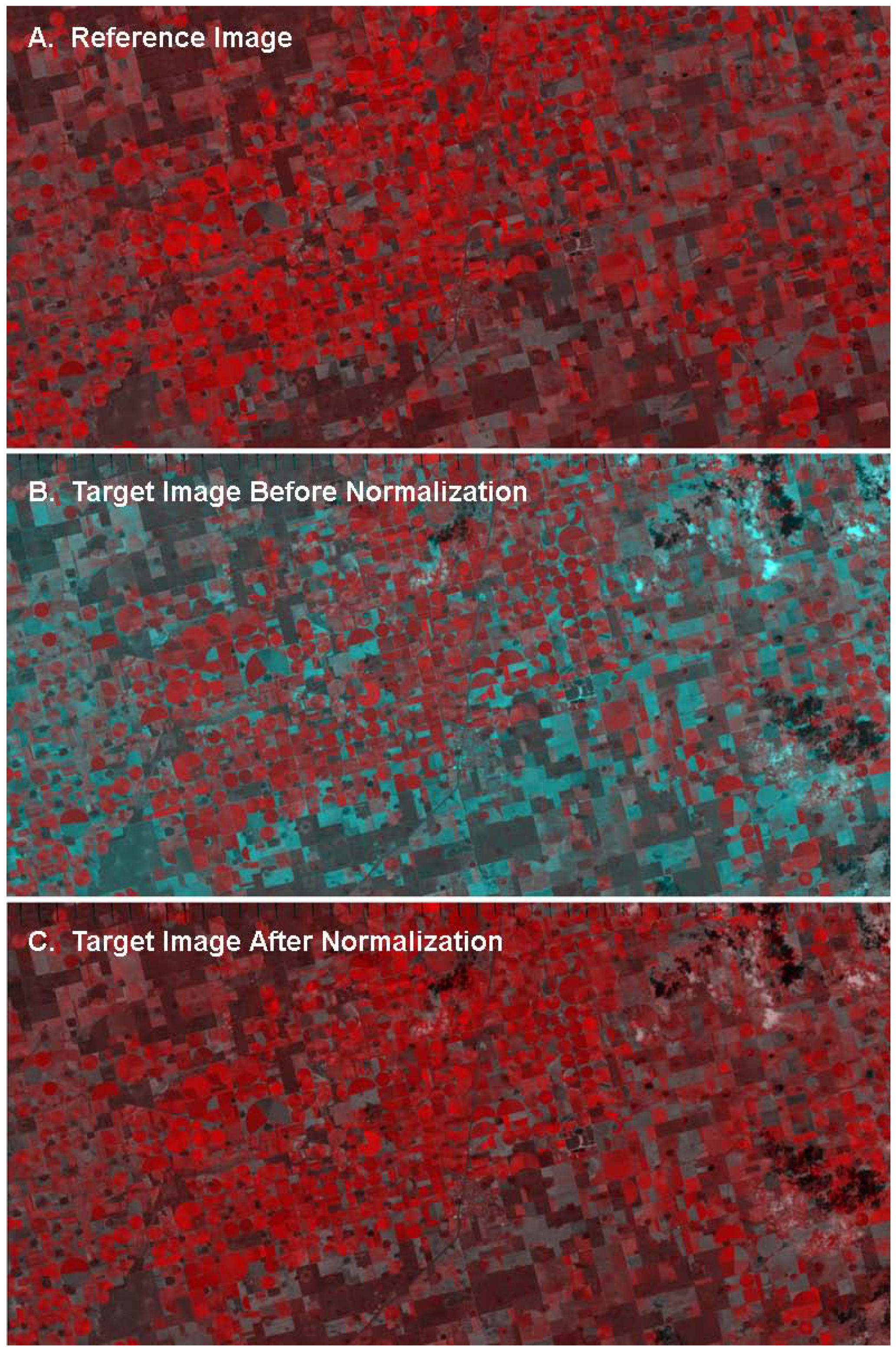
Figure 5. Red-NIR scatterplots for the Landsat image sections used in demonstrating the image normalization procedure (A) Reference image. (B) Target image before normalization. (C) Target image after normalization.

Figure 5. Red-NIR scatterplots for the Landsat image sections used in demonstrating the image normalization procedure (A) Reference image. (B) Target image before normalization. (C) Target image after normalization.

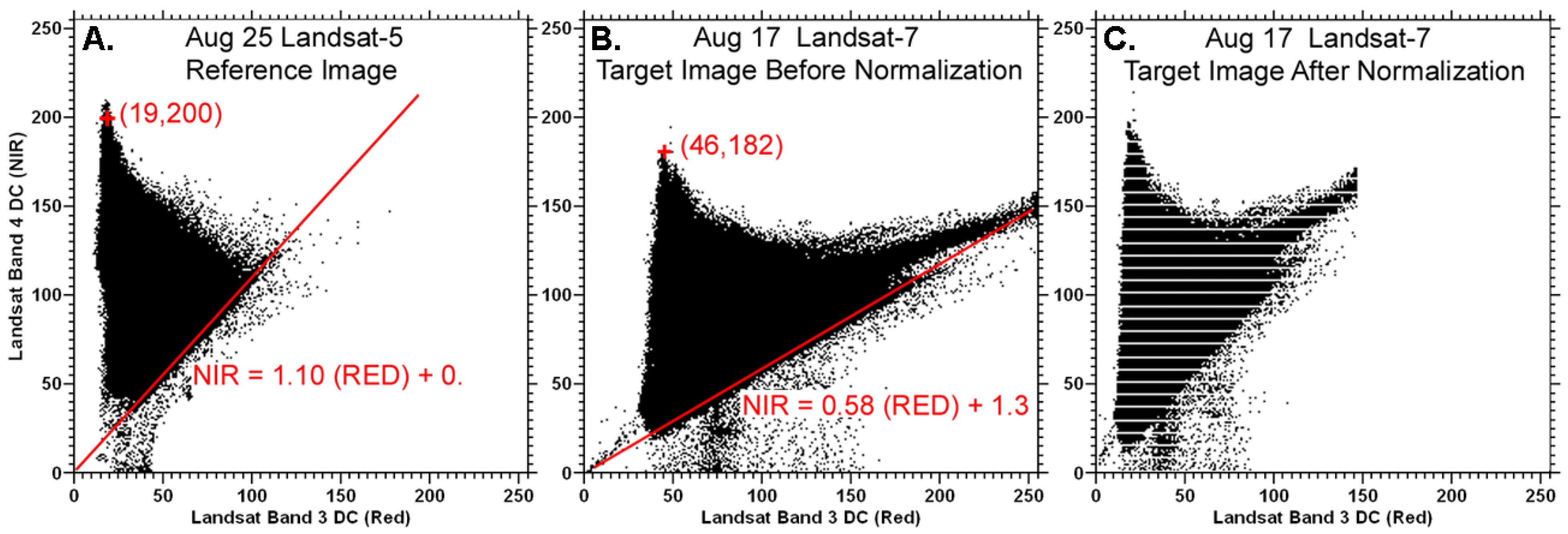
Figure 6. NIR-red scatter plot for the normalized target image overlaid with the scatter plot for the reference image.

Figure 6. NIR-red scatter plot for the normalized target image overlaid with the scatter plot for the reference image.

Ground-based measurements of leaf canopy reflectance in the NIR spectral band are plotted versus corresponding values in the red spectral band in Figure 8A,B for the seven plant species used in this study (Table 2). The average values in Figure 8A in the red spectral band cluster tightly between 2% and 5% reflectance. In the NIR, the average values extend over a range of reflectances, but with no value less than 50%. This distribution of points resembles the “spike” in the scatter plot between points c and d in Figure 1B representing the reflectance from vegetation at or above the canopy density necessary for full ground cover. In this situation, the coordinates of the FCP corresponding to point c would lie near the bottom of this distribution. Considering the overlap in the measurements indicated in Figure 8B, we took the average of the lower portion of this cluster of points (between 50% and 60% NIR reflectance) as a representative value for the FCP for a variety of plant species. This yielded a NIR coordinate value of 54.1% reflectance and a red coordinate value of 3.3% reflectance, respectively, for the FCP. This agrees with previous full-canopy reflectance measurements for cotton of 56% in the NIR spectral band and 4% in the red spectral band [22].

Figure 7. NIR versus red reflectance for the seven soils used in this study (refer to Table 1 for meanings of the symbols representing the soil names). Diagonal line passing through the points is the least-squares regression.

Figure 7. NIR versus red reflectance for the seven soils used in this study (refer to Table 1 for meanings of the symbols representing the soil names). Diagonal line passing through the points is the least-squares regression.

Results of analyzing the ground-based reflectance measurements in Figure 7 and Figure 8 provided the reference values for the BSL and FCP used in converting the May 13 and May 29 Landsat TM target images from DC to surface reflectance. DC scatter plots for these two images are presented in Figure 9. The equations for the BSL in these two images are similar, as are the coordinates of the FCP.

The results presented in Figure 10 involving observed and estimated values of surface reflectance for the six ground sites (Table 3 and Figure 3) can be used to assess the effectiveness of this conversion. In general, the points in the graph tend to cluster along the 1:1 line. The linear regression fit through these points explains over 95% of their variation. Statistical analysis of this regression line indicates that its slope (1.117) is not significantly different from 1 (t = 1.54, α = 0.05, 10 df), and that its intercept (−2.732) is not significantly different from 0 (t = 0.619, α = 0.05, 10 df). This suggests that the regression line is not significantly different from the 1:1 line. The mean estimated reflectance for the combined set of NIR and red values was 20.6%, while the corresponding value for the mean observed reflectance was 20.9%. Statistical analysis showed that these two means were not significantly different (t = 0.006, α = 0.05, 22 df). These results suggest that the conversion from DC to surface reflectance for the two target images was effective. On average, the estimated reflectance values were within 2.5% of the corresponding observed reflectance values, which could be interpreted as a rough estimate of the accuracy of the SPM conversion.

Figure 8. NIR versus red leaf canopy reflectance for the seven plant species used in this study. (A) Average values for each data set. (B) Detailed view of the cluster of values. Error bars represent plus or minus one standard deviation about the mean.

Figure 8. NIR versus red leaf canopy reflectance for the seven plant species used in this study. (A) Average values for each data set. (B) Detailed view of the cluster of values. Error bars represent plus or minus one standard deviation about the mean.

Figure 9. DC scatter plots for the May 13 and May 29 Landsat TM target images.

Figure 9. DC scatter plots for the May 13 and May 29 Landsat TM target images.

Figure 10. Observed values of surface reflectance in the NIR and red spectral bands for the six ground sites (see Table 3) plotted versus corresponding estimated values extracted from the May 13 and May 29 Landsat TM images following their conversion to reflectance. The solid diagonal line represents the 1:1 line, while the dashed line is the least-squares linear regression fit to the points. Error bars represent plus or minus one standard deviation about the mean of the observed values.

Figure 10. Observed values of surface reflectance in the NIR and red spectral bands for the six ground sites (see Table 3) plotted versus corresponding estimated values extracted from the May 13 and May 29 Landsat TM images following their conversion to reflectance. The solid diagonal line represents the 1:1 line, while the dashed line is the least-squares linear regression fit to the points. Error bars represent plus or minus one standard deviation about the mean of the observed values.

4.2. Strengths and Weaknesses of the SPM Method

The examples presented in the previous sections demonstrate that SPM can be an effective method for normalizing one remote sensing image to another, or for converting the DC values in an image to surface reflectance. Since SPM is an image-based method, it does not require the collection of information in addition to the image data, as with physically based approaches. SPM does not require the identification of specific “pseudo-invariant objects” in the imagery, such as deep clear lakes or man-made objects. The method also avoids the use of bright and dark PIFs in the imagery, which also may be absent. SPM is well-suited for application to imagery of agricultural and other vegetated regions, since it relies on PIFs related to soil and plant canopies. These PIFs can almost always be identified within the NIR-red scatter plots for such imagery, and their identification is not hindered by the presence of scattered clouds and cloud shadows in the imagery. Finally, the mathematical computations needed to perform SPM are simple and straight-forward.

A few aspects of the current form of SPM described in this article might be considered weaknesses. This current form of SPM only involves the NIR and red spectral bands of multispectral imagery. For many applications involving the quantification of vegetation characteristics (which primarily involves these two spectral bands), this may be adequate. Further research may show a way to extend the method to other spectral bands. In this article, we determined the BSL and FCP by visual inspection of the scatter plot. While this subjective approach may be adequate for many applications, it would be advantageous to have an objective method that could be generally applied for identifying the BSL and FCP in the scatter plot. We are aware of a proprietary, automated method that has been developed for doing this [23]. While SPM can correct for the effects of atmospheric transmissivity and path radiance (which in SPM are assumed to be uniform over an image), it cannot correct for adjacency effects (cross-radiance and cross-irradiance) associated with the relative brightness of the target and its surroundings [24]. Since adjacency effects are spatially non-uniform, they are a problem for most image-based normalization or conversion methods. Finally, a feature representing the FCP may not be present even for imagery of agricultural regions during certain times of the year. This usually occurs in the winter or early spring for a region that supports only warm-season crops. It still may be possible to identify a FCP at these times if there is sufficient natural vegetation in the region that maintains a leaf canopy during the colder periods.

5. Conclusions

Scatter Plot Matching (SPM) represents an effective and relatively simple method for normalizing one remote sensing image to another, or for converting image DC values to surface reflectance. It is particularly well-suited for application to imagery of agricultural and other vegetated regions which might not contain bright and dark pseudo-invariant objects or features such as deep lakes or large man-made objects. SPM is flexible in that the reference information needed to transform a target image can come from another image or from ground-based measurements. While the current form of this approach has certain weaknesses, continued research may lead to improvements that increase the accuracy and applicability of the method.

References

- Lu, D.; Mausel, P.; Brondizio, E.; Moran, E. Assessment of atmospheric correction methods for Landsat TM data applicable to Amazon basin LBA research. Int. J. Remote Sens. 2002, 23, 2651–2671. [Google Scholar] [CrossRef]
- Chander, G.; Markham, B. Revised Landsat-5 TM radiometric calibration procedures and postcalibration dynamic ranges. IEEE Trans. Geosci. Remote Sens. 2003, 41, 2674–2677. [Google Scholar] [CrossRef]
- Moran, M.S.; Jackson, R.D.; Slater, P.N.; Teillet, P.M. Evaluation of simplified procedures for retrieval of land surface reflectance factors from satellite sensor output. Remote Sens. Environ. 1992, 41, 169–184. [Google Scholar] [CrossRef]
- Chavez, P.S., Jr. Image-based atmospheric corrections—Revisited and improved. Photogramm. Eng. Remote Sens. 1996, 62, 1025–1036. [Google Scholar]
- Mahiny, A.S.; Turner, B.J. A comparison of four common atmospheric correction methods. Photogramm. Eng. Remote Sens. 2007, 73, 361–368. [Google Scholar] [CrossRef]
- Kruse, A.F. Comparison of ATREM, ACORN, and FLAASH atmospheric corrections using low-altitude AVIRIS data of Boulder, Colorado. In Proceedings of the 13th JPL Airborne Geosciences Workshop, Pasadena, CA, USA, March 31–April 2, 2004.
- Moran, M.S.; Clarke, T.R.; Qi, J.; Barnes, E.M.; Pinter, P.J., Jr. Practical techniques for conversion of airborne imagery to reflectances. In Proceedings of the 16th Biennial Workshop on Videography and Color Photography in Resource Assessment, Weslaco, TX, USA, April 29–May 1, 1997; pp. 82–95.
- Ahern, F.J.; Goodenough, D.G.; Jain, S.C.; Rao, V.R.; Rochon, G. Use of clear lakes as standard reflectors for atmospheric measurements. In Proceedings of the 11th Int. Symposium on Remote Sensing of Environment, Ann Arbor, MI, USA, 1977; pp. 731–755.
- Chavez, P.S., Jr. An improved dark-object subtraction technique for atmospheric scattering correction of multispectral data. Remote Sens. Environ. 1988, 24, 459–479. [Google Scholar] [CrossRef]
- Chavez, P.S., Jr. Radiometric calibration of Landsat Thematic Mapper multispectral images. Photogramm. Eng. Remote Sens. 1989, 55, 1285–1294. [Google Scholar]
- Schott, J.R.; Salvaggio, C.; Volchok, W.J. Radiometric scene normalization using pseudoinvariant features. Remote Sens. Environ. 1988, 26, 1–16. [Google Scholar] [CrossRef]
- Hall, F.G.; Strebel, D.E.; Nickeson, J.E.; Goetz, S.J. Radiometric rectification: Toward a common radiometric response among multidate, multisensory images. Remote Sens. Environ. 1991, 35, 11–27. [Google Scholar] [CrossRef]
- Kauth, R.J.; Thomas, G.S. The Tasseled Cap—A graphic description of the spectral-temporal development of agricultural crops as seen by Landsat. In Proceedings of the Symposium on Machine Processing of Remotely Sensed Data, West Lafayette, IN, USA, June 29–July 1, 1976.
- Jensen, J.R. Remote Sensing of the Environment, an Earth Resource Perspective; Prentice-Hall: Upper Saddle River, NJ, USA, 2000; p. 343. [Google Scholar]
- Liang, S. Quantitative Remote Sensing of Land Surfaces; John Wiley and Sons: New York, NY, USA, 2004; p. 249. [Google Scholar]
- Gausman, H.W. Plant Leaf Optical Properties in Visible and Near-infrared Light; Texas Tech Press: Lubbock, TX, USA, 1985. [Google Scholar]
- Price, J.C. Calibration of satellite radiometers and the comparison of vegetation indices. Remote Sens. Environ. 1987, 21, 15–27. [Google Scholar] [CrossRef]
- USGS/EROS. SLC-off Information. Available online: http://landsat.usgs.gov/products_slc_off_data_information.php (accessed on 22 June 2010).
- Maas, S.J.; Rajan, N. Estimating ground cover of field crops using medium-resolution multispectral satellite imagery. Agron. J. 2008, 100, 320–327. [Google Scholar] [CrossRef]
- Jackson, R.D.; Pinter, P.J., Jr.; Reginato, R.J.; Idso, S.B. Hand-Held Radiometry; Publication ARM-W-19; US Dept. of Agriculture: Phoenix, AZ, USA, 1980. [Google Scholar]
- Huete, A.R.; Post, D.F.; Jackson, R.D. Soil spectral effects on 4-space vegetation discrimination. Remote Sens. Environ. 1984, 15, 155–165. [Google Scholar] [CrossRef]
- Maas, S.J. Structure and reflectance of irrigated cotton leaf canopies. Agron. J. 1997, 89, 54–59. [Google Scholar] [CrossRef]
- Schulthess, Urs. Personal communication, RapidEye AG: Brandenburg, Germany, March 2010.
- Otterman, J.; Ungar, S.; Kaufman, Y.; Podolak, M. Atmospheric effects on radiometric imaging from satellites under low optical thickness conditions. Remote Sens. Environ. 1980, 9, 115–129. [Google Scholar] [CrossRef]
© 2010 by the authors; licensee MDPI, Basel, Switzerland. This article is an open access article distributed under the terms and conditions of the Creative Commons Attribution license (http://creativecommons.org/licenses/by/3.0/).
Share and Cite
MDPI and ACS Style
Maas, S.J.; Rajan, N. Normalizing and Converting Image DC Data Using Scatter Plot Matching. Remote Sens. 2010, 2, 1644-1661. https://doi.org/10.3390/rs2071644
AMA Style
Maas SJ, Rajan N. Normalizing and Converting Image DC Data Using Scatter Plot Matching. Remote Sensing. 2010; 2(7):1644-1661. https://doi.org/10.3390/rs2071644
Chicago/Turabian StyleMaas, Stephan J., and Nithya Rajan. 2010. "Normalizing and Converting Image DC Data Using Scatter Plot Matching" Remote Sensing 2, no. 7: 1644-1661. https://doi.org/10.3390/rs2071644