Retrieval of Leaf Area Index (LAI) and Soil Water Content (WC) Using Hyperspectral Remote Sensing under Controlled Glass House Conditions for Spring Barley and Sugar Beet

Abstract

Leaf area index (LAI) and water content (WC) in the root zone are two major hydro-meteorological parameters that exhibit a dominant control on water, energy and carbon fluxes, and are therefore important for any regional eco-hydrological or climatological study. To investigate the potential for retrieving these parameter from hyperspectral remote sensing, we have investigated plant spectral reflectance (400–2,500 nm, ASD FieldSpec3) for two major agricultural crops (sugar beet and spring barley) in the mid-latitudes, treated under different water and nitrogen (N) conditions in a greenhouse experiment over the growing period of 2008. Along with the spectral response, we have measured soil water content and LAI for 15 intensive measurement campaigns spread over the growing season and could demonstrate a significant response of plant reflectance characteristics to variations in water content and nutrient conditions. Linear and non-linear dimensionality analysis suggests that the full band reflectance information is well represented by the set of 28 vegetation spectral indices (SI) and most of the variance is explained by three to a maximum of eight variables. Investigation of linear dependencies between LAI and soil WC and pre-selected SI’s indicate that: (1) linear regression using single SI is not sufficient to describe plant/soil variables over the range of experimental conditions, however, some improvement can be seen knowing crop species beforehand; (2) the improvement is superior when applying multiple linear regression using three explanatory SI’s approach. In addition to linear investigations, we applied the non-linear CART (Classification and Regression Trees) technique, which finally did not show the potential for any improvement in the retrieval process.

1. Introduction

The quantitative description of water, carbon and energy fluxes between the land surface and the atmosphere plays an important role in current hydrological and climate research studies, especially at larger spatial scales [1]. An effective tool to derive relevant land surface characteristics over the last decades has been the development and use of satellite remote sensing techniques in the visible (VIS: 350–700 nm) and near infrared (NIR: 700–1,300 nm), short wave infrared (SWIR: 1,300–2,500 nm), microwave and thermal infrared spectral region of the electromagnetic spectrum (see e.g., [2] for an extensive review of methods in the field of eco-hydrology). In particular, the monitoring of narrow band spectral reflectance from plant surfaces using multi- and hyper-spectral sensors has proven very promising in gathering a large variety of eco-physiological information including photosynthetic activity (absorbed photosynthetically active radiation, APAR) [3], vegetation structure (leaf area index, LAI) [3,4], biomass and ecosystem productivity (net ecosystem productivity/gross primary productivity, NEP/GPP) [5], plant/leaf water content [6] or vegetation light use efficiency (LUE) [7], which is the ratio of GPP to APAR and controlled by the phenological stage, solar radiation conditions and the availability of soil moisture and nutrients [8].

The relationship between spectral reflectance and ecophysiological characteristics is often modeled via the use of spectral indices (SI’s) that are calculated from spectral reflectance of multiple bands. There have been a large number of investigations over the last years and a summary of developed and applied SI’s is given in Table 1. Spectral indices are here grouped into three major classes:

• The first group, including the normalized differential vegetation index (NDVI) as the most prominent representative, shows response to the general greenness, biomass and structure of the vegetation. The NDVI and its variants have successfully been related to properties such as the leaf area index (LAI), the fraction of absorbed photosynthetically active radiation (FPAR) or the biomass of many different ecosystems and environments [9,10].
• The second group of indices is related to the leaf pigment activity (such as xanthophyll or carotenoid) that shows sensitivity to plant physiological processes and in particular to the photosynthetic radiation use efficiency, a major component in many current eco-climatic models and analysis. Specifically, the photochemical reflectance index (PRI, the normalized difference of the 531 and 570 nm bands) has received large attention over the last years allowing relating spectral response to carbon fluxes and GPP [7,11,12,13]. As the PRI is sensitive to the plant xanthophyll cycle, active when dissipating excess energy under intensive radiation, and also dependent on water and nutrient availability, it will be a very useful indicator of the soil moisture and nutrient regime at a particular location [6,14].
• The third group of indices mainly uses water absorption bands in the near- and mid-infrared region. They are sensitive to the leaf/plant water concentration that is controlled by the soil water availability and climatic conditions. A detailed discussion about pros and cons of individual spectral bands/indices can be found in [6,15,16]. In general, the indices of this group are applied in areas such as drought assessment, irrigation practice or wild fire risk [17].

Table 1. List of SI’s to describe plant ecophysiological parameters reviewed from the literature and used throughout this paper. SI’s are grouped into three general classes showing response to (a) greenness, biomass and structure of the vegetation, (b) light use efficiency, and (c) vegetation and leaf water content. R_xxx indicates the reflectance at a specific wavelength (nm).

Spectral Index	Index Name	Equation	Reference
Greenness/Biomass/Canopy structure:
NDVI_a	Normalized Difference Vegetation Index–variant A	NDVI_a = (R800 − R670) / (R800 + R670)	[7,9]
2. NDVI_b	Normalized Difference Vegetation Index–variant B	NDVI_b = (R858−R648) / ( R858 + R648)	[18]
3. RDVI	Renormalized Difference Vegetation Index	RDVI = (R800−R670) / sqrt (R800 + R670)	[19]
4. NDVI_705	Red Edge Normalized Difference Vegetation Index	NDVI_705 = (R750−R705) / (R750 + R705)	[20,21]
5. mNDVI_705	Modified Red Edge Normalized Difference Vegetation Index	mNDVI_705 = (R750 − R705)/ (R750 + R705 − 2R445)	[21,22]
6. RNDVI	Red Normalized Difference Vegetation Index	RNDVI = (R780 − R670) / ( R780 + R670)	[10,23]
7. GNDVI	Green Normalized Difference Vegetation Index	GNDVI = (R780 − R550) / ( R780 + R550)	[23,24]
8. MSR	Modified Simple Ratio	MSR = ((R800/R670) − 1) / sqrt ((R800/R670) + 1)	[19,25]
9. SR _680_a	Narrowband Simple Ratio 680–variant A	SR_680_a = R800 / R680	[21]
10. SR _680_b	Narrowband Simple Ratio 680–variant B	SR_680_b = R900 / R680	[26]
11. SR _705	Narrowband Simple Ratio 705	SR_705 = R750 / R705	[21]
12. mSR_680	Modified Simple Ratio 680	mSR_680 = (R800 − R445) / ( R680 − R445)	[21,22]
13. mSR_705	Modified Simple Ratio 705	mSR_705 = (R750 − R445) / ( R705 − R445)	[21]
14. RG	Narrowband Red Green Ratio	RG = ∑(R600:R699) / ∑(R500:R599)	[21]
Pigment activity/Light Use Efficiency:
15. PRI	Photochemical Reflectance Index	PRI = (R531 − R570) / ( R531 + R570)	[12,13,14]
16. SIPI	Structure Intensive Pigment Index	SIPI = (R800 − R445) / ( R800 + R680)	[14]
17. NPCI	Normalized Pigments Reflectance Index	NPCI = (R680 − R430) / (R680 + R430)	[14]
18. PSRI	Plant Senescence Reflectance Index	PSRI = (R680 − R500) / R750	[21,27]
Water indices:
19. NDWI_1241	Normalized Difference Water Index R1241	NDWI_1241 = (R857 − R1241) / ( R857 + R1241)	[15]
20. NDWI_1640	Normalized Difference Water Index R1640	NDWI_1640 = (R857 − R1640) / ( R857 + R1640)	[18]
21. NDWI_2130	Normalized Difference Water Index R2130	NDWI_2130 = (R857 − R2130) / ( R857 + R2130)	[18]
22. WBI	Water Band Index	WBI = R900 / R970	[28,29]
23. RATIO 975	Three-band ratio 975	RATIO_975 = 2∑(R960:R990) / (∑(R920:R940) + ∑(R1090:R1110))	[30]
24. RATIO 1200	Three-band ratio 1200	RATIO_1200 = 2∑(R1180:R1220) / (∑(R1090:R1110) + ∑(R1265:R1285))	[30]
25. MSI	Moisture Stress Index	MSI = R1599 / R819	[16,31]
26. NDII	Normalized Difference Infrared Index	NDII = (R819 − R1649) / ( R819 + R1649)	[32,33]
27. NWI_1	Normalized Water Index 1	NWI1 = (R970 − R900) / (R970 + R900)	[23]
28. NWI_2	Normalized Water Index 2	NWI1 = (R970 − R850) / (R970+R850)	[23]

Table 1. List of SI’s to describe plant ecophysiological parameters reviewed from the literature and used throughout this paper. SI’s are grouped into three general classes showing response to (a) greenness, biomass and structure of the vegetation, (b) light use efficiency, and (c) vegetation and leaf water content. R_xxx indicates the reflectance at a specific wavelength (nm).

Spectral Index	Index Name	Equation	Reference
Greenness/Biomass/Canopy structure:
NDVI_a	Normalized Difference Vegetation Index–variant A	NDVI_a = (R800 − R670) / (R800 + R670)	[7,9]
2. NDVI_b	Normalized Difference Vegetation Index–variant B	NDVI_b = (R858−R648) / ( R858 + R648)	[18]
3. RDVI	Renormalized Difference Vegetation Index	RDVI = (R800−R670) / sqrt (R800 + R670)	[19]
4. NDVI_705	Red Edge Normalized Difference Vegetation Index	NDVI_705 = (R750−R705) / (R750 + R705)	[20,21]
5. mNDVI_705	Modified Red Edge Normalized Difference Vegetation Index	mNDVI_705 = (R750 − R705)/ (R750 + R705 − 2R445)	[21,22]
6. RNDVI	Red Normalized Difference Vegetation Index	RNDVI = (R780 − R670) / ( R780 + R670)	[10,23]
7. GNDVI	Green Normalized Difference Vegetation Index	GNDVI = (R780 − R550) / ( R780 + R550)	[23,24]
8. MSR	Modified Simple Ratio	MSR = ((R800/R670) − 1) / sqrt ((R800/R670) + 1)	[19,25]
9. SR _680_a	Narrowband Simple Ratio 680–variant A	SR_680_a = R800 / R680	[21]
10. SR _680_b	Narrowband Simple Ratio 680–variant B	SR_680_b = R900 / R680	[26]
11. SR _705	Narrowband Simple Ratio 705	SR_705 = R750 / R705	[21]
12. mSR_680	Modified Simple Ratio 680	mSR_680 = (R800 − R445) / ( R680 − R445)	[21,22]
13. mSR_705	Modified Simple Ratio 705	mSR_705 = (R750 − R445) / ( R705 − R445)	[21]
14. RG	Narrowband Red Green Ratio	RG = ∑(R600:R699) / ∑(R500:R599)	[21]
Pigment activity/Light Use Efficiency:
15. PRI	Photochemical Reflectance Index	PRI = (R531 − R570) / ( R531 + R570)	[12,13,14]
16. SIPI	Structure Intensive Pigment Index	SIPI = (R800 − R445) / ( R800 + R680)	[14]
17. NPCI	Normalized Pigments Reflectance Index	NPCI = (R680 − R430) / (R680 + R430)	[14]
18. PSRI	Plant Senescence Reflectance Index	PSRI = (R680 − R500) / R750	[21,27]
Water indices:
19. NDWI_1241	Normalized Difference Water Index R1241	NDWI_1241 = (R857 − R1241) / ( R857 + R1241)	[15]
20. NDWI_1640	Normalized Difference Water Index R1640	NDWI_1640 = (R857 − R1640) / ( R857 + R1640)	[18]
21. NDWI_2130	Normalized Difference Water Index R2130	NDWI_2130 = (R857 − R2130) / ( R857 + R2130)	[18]
22. WBI	Water Band Index	WBI = R900 / R970	[28,29]
23. RATIO 975	Three-band ratio 975	RATIO_975 = 2∑(R960:R990) / (∑(R920:R940) + ∑(R1090:R1110))	[30]
24. RATIO 1200	Three-band ratio 1200	RATIO_1200 = 2∑(R1180:R1220) / (∑(R1090:R1110) + ∑(R1265:R1285))	[30]
25. MSI	Moisture Stress Index	MSI = R1599 / R819	[16,31]
26. NDII	Normalized Difference Infrared Index	NDII = (R819 − R1649) / ( R819 + R1649)	[32,33]
27. NWI_1	Normalized Water Index 1	NWI1 = (R970 − R900) / (R970 + R900)	[23]
28. NWI_2	Normalized Water Index 2	NWI1 = (R970 − R850) / (R970+R850)	[23]

In the following, we want to explore the potential of using hyperspectral indices in order to derive two important land surface parameters most relevant to eco-hydrological applications: (i) LAI, related to vegetation biomass and height, thereby influencing surface roughness and providing exchange area for ecosystem gas and energy transport processes between the vegetation and the atmosphere [34]; also LAI is used as a proxy for the vegetation interception storage, thus controlling important components of the hydrological cycle; and (ii) the availability of root zone soil moisture, being a dominant control on ecosystem water vapor and carbon fluxes, biomass production and crop yield [35].

While both, LAI and root zone WC, are increasingly derived using the inversion of canopy reflectance models in the visible and infrared (LAI, see [36] for an overview) and in the microwave spectral region (WC, e.g., [37,38,39]), we here want to restrict our analysis to the use of hyperspectral reflectance data and in particular to the use of individual narrow band ratios (Table 1). There are two main reasons for this: First, the use of simple SI’s will be significantly less demanding in terms of computational resources when compared to the inversion of radiation transfer models such as PROSAIL [40] and might therefore be necessary for product development, e.g., with the launch of EnMAP (Environmental Mapping and Analysis Program) envisaged for 2013. Also, the use of simple indices would allow, e.g., the applications of low cost camera systems including narrow band optical filters serving as an alternative for cheap and widespread application.

Therefore, one major aim of this study is to find the most significant and lowest dimensional spectral band combinations for extracting the LAI and WC. We have investigated two major agricultural crops in the mid-latitudes, namely sugar beet and spring barley, under different water and N-treatments in a greenhouse environment over the vegetation period of 2008. Different water and N-treatments will allow a broad spectrum of environmental conditions to be explored. Section 2 will describe the experimental setup, the used instruments, and the measured variables in more detail. Section 3 presenting the experimental results gives an extensive analysis of the temporal dynamics of differences in spectral reflectance for different experimental conditions. Here, we also try to extract the dominant spectral ranges and vegetation indices that allow soil moisture content in the root zone and N conditions to be derived from remote sensing. In particular we would like to derive and test an empirical relationship between spectral reflectance information and the soil WC and LAI. This is followed by a discussion and conclusion in Section 4.

2. Experimental Design

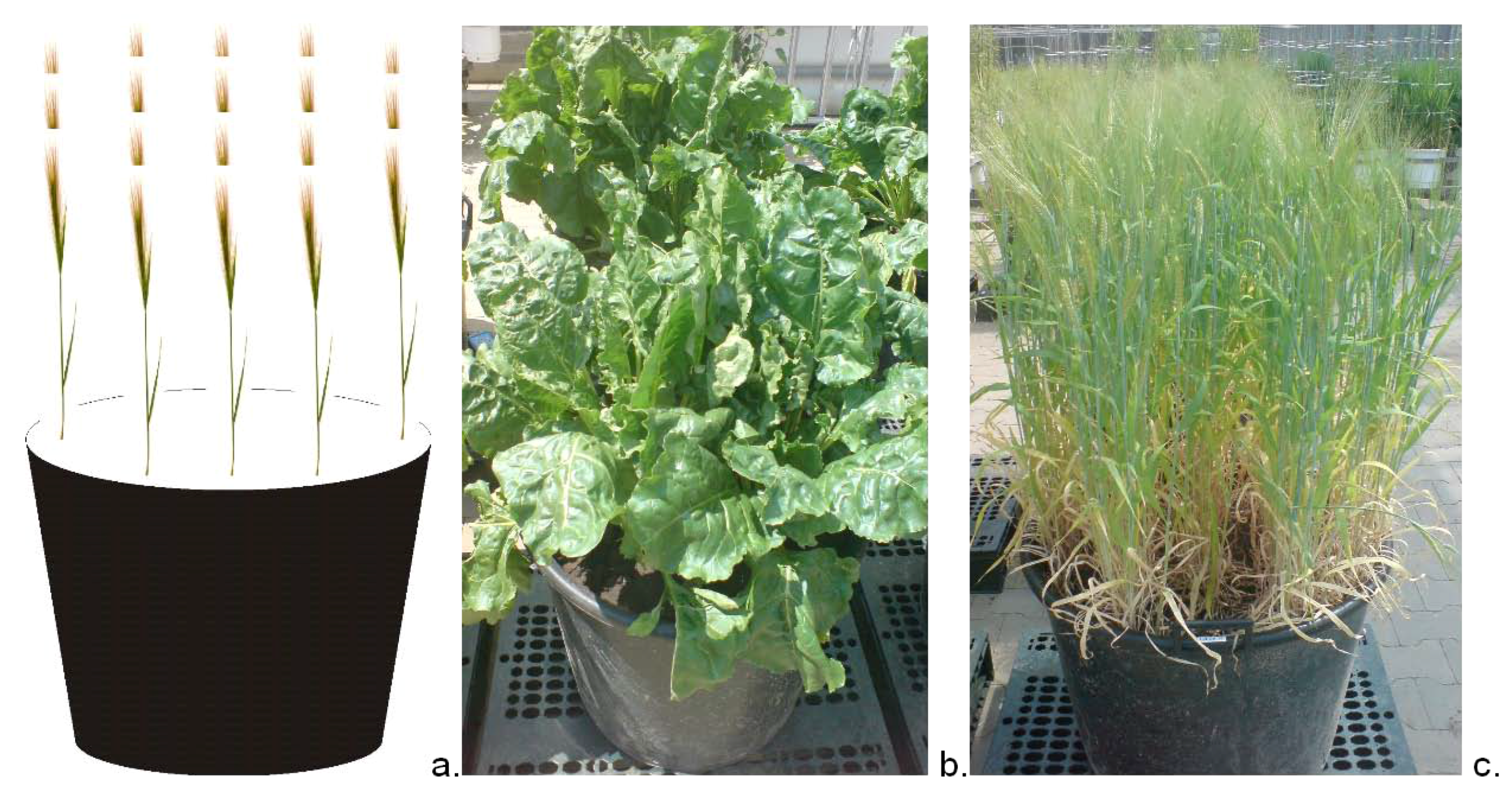
2.1. Study Site and Experimental Setup

Experimental data have been obtained during the growing season 2008 at the field research station of the UFZ-Helmholtz Centre for Environmental Research in Bad Lauchstädt (BL), Saxony-Anhalt, Germany (51°23′32″N 11°52′33″E, altitude 113 m a.s.l., mean annual precipitation 484 mm, mean annual temperature 8.7 °C; [41]). Two main German agricultural crop species, spring barley (Hordeum vulgare L.) and sugar beet (Beta vulgaris ssp.), were chosen as objects of investigation. A total of 24 pots were planted using black soil in circular-shaped pots, 0.6 m in diameter and 0.8 m high, 12 for spring barley and 12 for sugar beet. There were four sugar beet plants per pot and spring barley was planted in rows, allowing five rows per pot separated by 0.125 m as illustrated in Figure 1.

Figure 1. Schematic (a) and example pots for sugar beet (b) and barley (c) (18.06.2008).

Figure 1. Schematic (a) and example pots for sugar beet (b) and barley (c) (18.06.2008).

Selected crops were seeded and grown in the winter greenhouse equipped with removable walls and roof that were left open during the day and closed during the night and rainfall events. This allowed plant growth under most possible natural environment conditions while being able to examine crop response to artificially produced water stress under different nutrient conditions. After seeding at the beginning/mid of April, all pots were initially cultivated under normal, well watered conditions (defined by 60% of soil field capacity that has been derived from 24 h capillary saturation of 100 cm³ soil cores, and 2 h ex-filtration on a 6 cm sandbed). The spectral and other measurements under controlled conditions started in the first week of June when soil/plot covering by plants was almost complete. Spring barley was in the flowering stage roughly 6–7 weeks after first emergence. For sugar beet the measurements started when 4–6 leaves were unrolled and fully developed. Table 2 gives a detailed overview about phenological stages and the time schedule of the experiment.

Table 2. Time schedule of the Bad Lauchstädt Experiment 2008. Black vertical pointers indicate in which part of the month particular events took place.

Spring Barley

seeding

first emergence

flowering

beginning of experiment

end of experiment

March

April

May

June

July

seeding

first emergence

4–6 leaves unrolled

beginning of experiment

end of experiment

Sugar Beet

Table 2. Time schedule of the Bad Lauchstädt Experiment 2008. Black vertical pointers indicate in which part of the month particular events took place.

Spring Barley

seeding

first emergence

flowering

beginning of experiment

end of experiment

March

April

May

June

July

seeding

first emergence

4–6 leaves unrolled

beginning of experiment

end of experiment

Sugar Beet

At the start of the experiment, pots were treated with different water and nutrient conditions. Two variants concerning nutrient treatment and three different modes of irrigation were considered. The Bad Lauchstädt soil used in this experiment is Haplic Chernozem (FAO classification) developed from loess [42] with 22% clay [41] characterized by a very high organic carbon (C_org = 19.8 g kg⁻¹) and total nitrogen (N_tot = 1.6 g kg⁻¹) contents [43]. Before seeding, all sample-pots were filled with 150 kg of soil material, 12 pots (six for sugar beet and six for spring barley) received an addition of mineral fertilizer, while the other 12 pots were kept as a reference without fertilizer. The amount of mineral fertilizer applied was defined in accordance with the “Standard Bad Lauchstädt” treatment praxis (15 g P and N as well as 20 g K per pot). The two fertilizer treatments are called “N-low” or “N-high” in the following. Three different water treatments have been applied defined as follows: a “high” WC was defined by controlling WC at a value of 60% of the soil field capacity, for a “medium” variant this value was set to 30% of field capacity, and “low” variant was defined by no additional water supply. The water status/content was verified every second–third day by weighting of the pots, followed by an irrigation to compensate for the evapotranspiration losses. In total, 24 pots including two different crop species under two nutrient and three irrigation treatments are considered and investigated, and each combination has two replicates.

2.2. Instrumentation and Measurements

Top of canopy spectral signatures were taken using the FieldSpec Pro 3 (Analytical Spectral Devices, Boulder, CO, USA) field portable spectrometer with a full spectral range located in the VIS, NIR and SWIR region (350–2,500 nm). Instrument sampling intervals (1.4 nm—VIS and NIR; 2 nm—SWIR) undergo an automatic internal interpolation to 1 nm spacing using linear and polynomial equations [44]. All spectral surveys were taken under two conditions: First, reflectance was recorded from nadir position about 0.45–0.55 m above the top of the plant under sun illumination in the winter greenhouse with all walls and the roof removed. Second, two tungsten halogen quartz lamps: THQ (Dörr, Neu-Ulm, Germany) with 1,000 watt, 3,200 K color temperature, 26,000 Lumens of brightness each (http://www.doerrfoto.de/) under closed room conditions were used. Both lamps were installed in a closed greenhouse room with walls covered with black mat paint. Lamps were pointed from two opposite directions and mounted at a 30° angle according to the floor plane. For reflectance scanning under THQ illumination, every sample pot had to be carried into the dark room using special lift truck designed to carry heavy load. Reference measurements were taken for both modes using a Spectralon (LabSphere, North Sutton, NH, USA) white reference panel (Effective Spectral Range: 250–2,500 nm, Reflectance within 400–1,500 nm: 99% and within 250–2,500 nm: more than 95%, Thermal Stability: up to 400 °C) at the beginning of each time series and after changes of sun illumination conditions under mode 1. Spectral data were collected throughout the experiment between 11:00 a.m. and 1:00 p.m. in order to avoid large impacts of bidirectional effects. Each reflectance spectra was calculated as an average over four individual spectral measurements (each averaged from 25 internal surveys) slightly varied around the pot center to avoid boundary effects per pot.

LAI was measured using a LAI 2,000 plant canopy analyzer (LI-COR, NE, USA) directly after the spectral measurement under outside but shadowed conditions. Measurements were carried out considering individual calibration of the instrument in a way that the hemispherical field of view was least influenced by the experimental setup and conditions. Again, each data set was averaged over four individual measurements per pot. Soil moisture was measured as volumetric soil WC using a ThetaProbe ML2x FD-probe (Delta-T Devices Ltd, Cambridge, UK) for every sampling day. A probe length of 60 mm and a set of 4–10 measurements per pot (with regards to possible soil penetration dependent on soil softness/dryness) guaranteed an average water content in the upper root zone of the pot. In addition, vegetation height, and in case of sugar beet: leaves length, were monitored.

The glasshouse experiment was started in the first week of June 2008 and was continued over a six weeks period until the second week of July. Measurements were taken at 15 individual dates however, as spectral reflectance measurements under outside conditions were limited due to unfavorable weather conditions, and as the reflectance spectra and derived SI’s did not show any significant differences between both illumination conditions, we have limited our further analysis to the use of data obtained under indoor conditions. Besides direct reflectance measurements, the 28 spectral indices as defined in Table 1 were calculated on the basis of averaged spectra.

3. Results

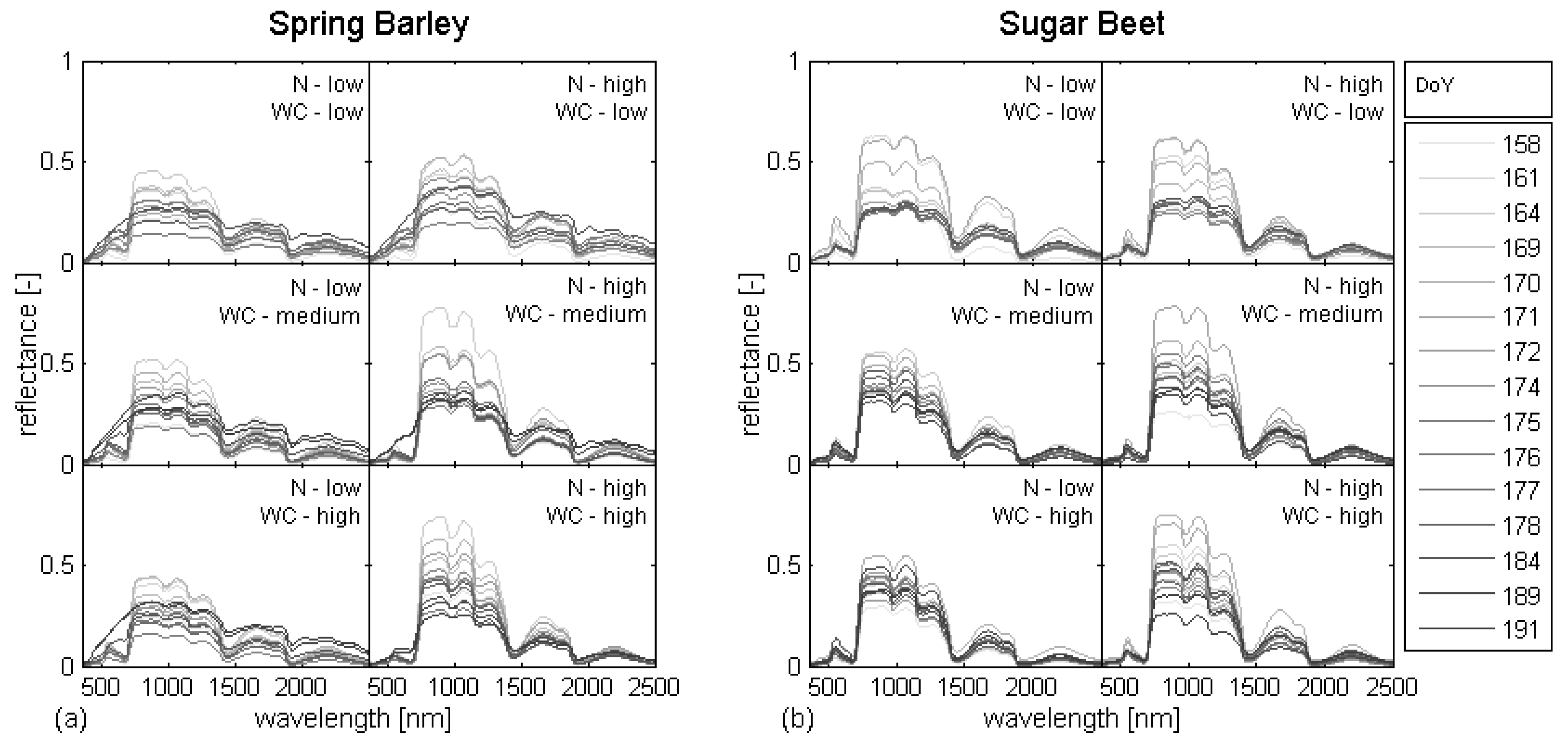
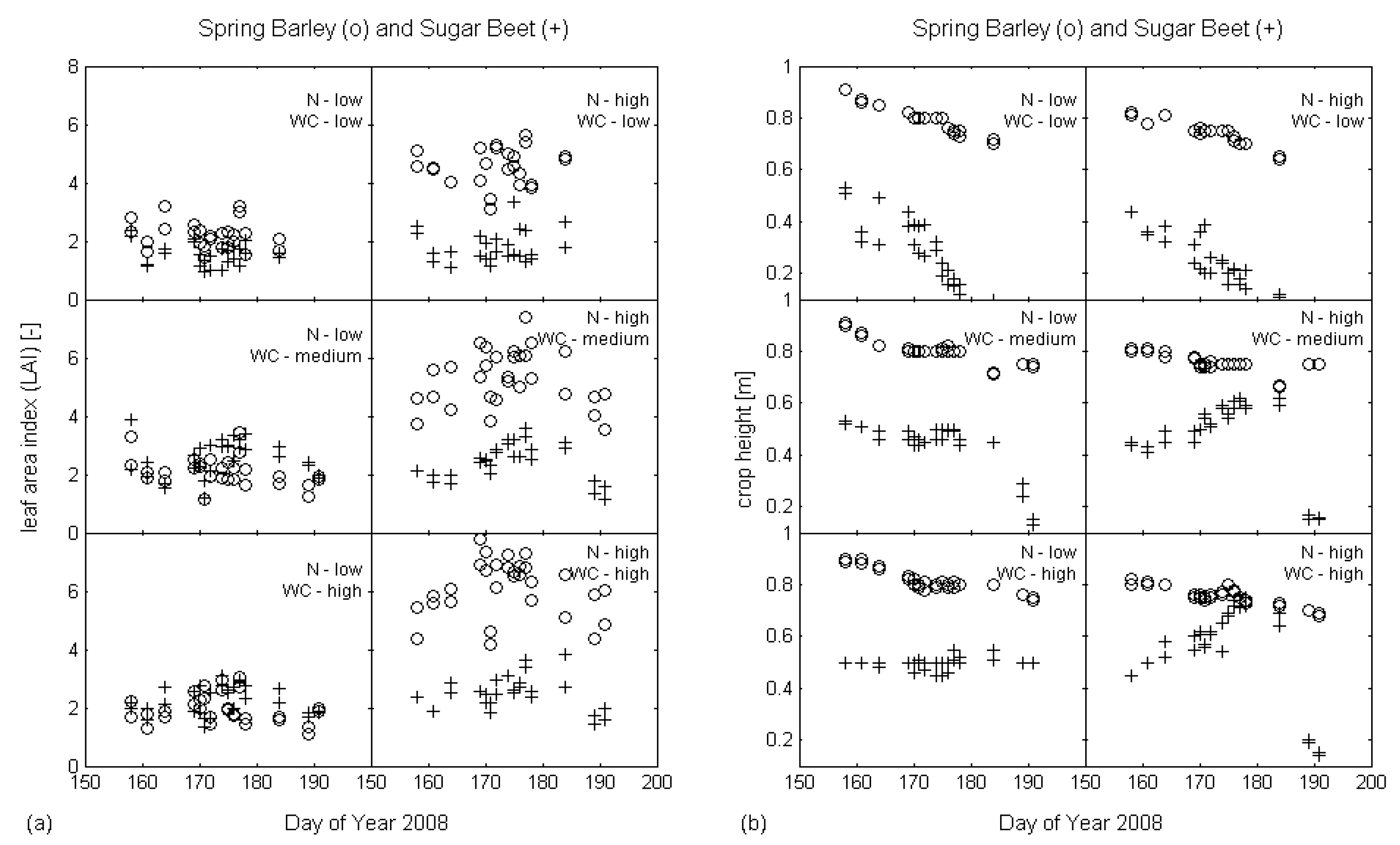
3.1. Dynamics of Plant Spectral and Biological Properties

Figure 2a and b show the temporal dynamics of reflectance properties for Spring Barley (a) and Sugar Beet (b) separately for all combinations of water (WC) and nitrogen (N) treatments. Spectra for each crop type/N-/WC-treatment combination vary not only between single time steps but also in between different N- and WC-treatments due to the changes in a canopy structure and differences in pigment and water content, both caused by different availability of water and nutrients. It is obvious from Figure 2 that spectral response significantly changes over time, however, to a different degree for different treatments and for different crop types. As pointed out by [45,46], spectral domains of strong chlorophyll (blue and red) and water (water bands) absorption are more sensitive to low concentration of chlorophyll and water, while others (green and regions between water bands) are more sensitive to high water and N-concentration. From the reflectance spectra in Figure 2, where we see both, a clear temporal development that seems to be dominated by the plant growth and therefore LAI dynamics, and (to a much smaller extent) differences under different irrigation conditions, we would expect at least some potential for the extraction of LAI and WC from narrow band SI’s.

Figure 2. Temporal dynamics of spectral properties of Spring Barley (a) and Sugar Beet (b), plotted with regards to applied WC and N treatments (indicated in an upper right corner of all plots), during the BL 2008 experiment.

Figure 2. Temporal dynamics of spectral properties of Spring Barley (a) and Sugar Beet (b), plotted with regards to applied WC and N treatments (indicated in an upper right corner of all plots), during the BL 2008 experiment.

Differences in plant development for different water and nutrient availability, as indicated by measured LAI values and crop height, are illustrated in Figure 3. As expected, samples under low N treatment (Figure 3a left) indicate low LAI values, while those cultivated under high N conditions (Figure 3a right) show higher values. However, this behavior is much more distinct for spring barley (o) than for sugar beet (+), where this difference grows with increasing water level. The analysis of crop height (Figure 3b) indicates a clear difference between both species. While different in their phenology, it can be observed that under low nitrogen conditions (Figure 3b left), the height for spring barley (o) decreases during the entire experiment and for all water levels. Sugar beet (+) height decreases very rapidly only under low water treatment, while under medium or high water conditions such behavior is only observable towards the end of the experiment. Interesting is the height development of spring barley under high nitrogen conditions (Figure 3b, right), where a decrease in height is similar to those under low nitrogen treatment.

In summary, plant spectral reflectance as well as the temporal development of LAI and crop height responds significantly to differences in water and nutrient availability. Even though reflectance sensitivity is not wavelength independent and varies within the entire spectral range, this behavior suggests the possibility of an inverse retrieval of crop characteristics and controlling water and nutrient conditions. This potential will be explored in the next sub-sections.

Figure 3. Temporal development of leaf area index (a) and of vegetation height (b) for Spring Barley (o) and Sugar Beet (+), plotted with regards to applied WC and N treatments (indicated in an upper right corner of all plots), BL 2008 Experiment.

Figure 3. Temporal development of leaf area index (a) and of vegetation height (b) for Spring Barley (o) and Sugar Beet (+), plotted with regards to applied WC and N treatments (indicated in an upper right corner of all plots), BL 2008 Experiment.

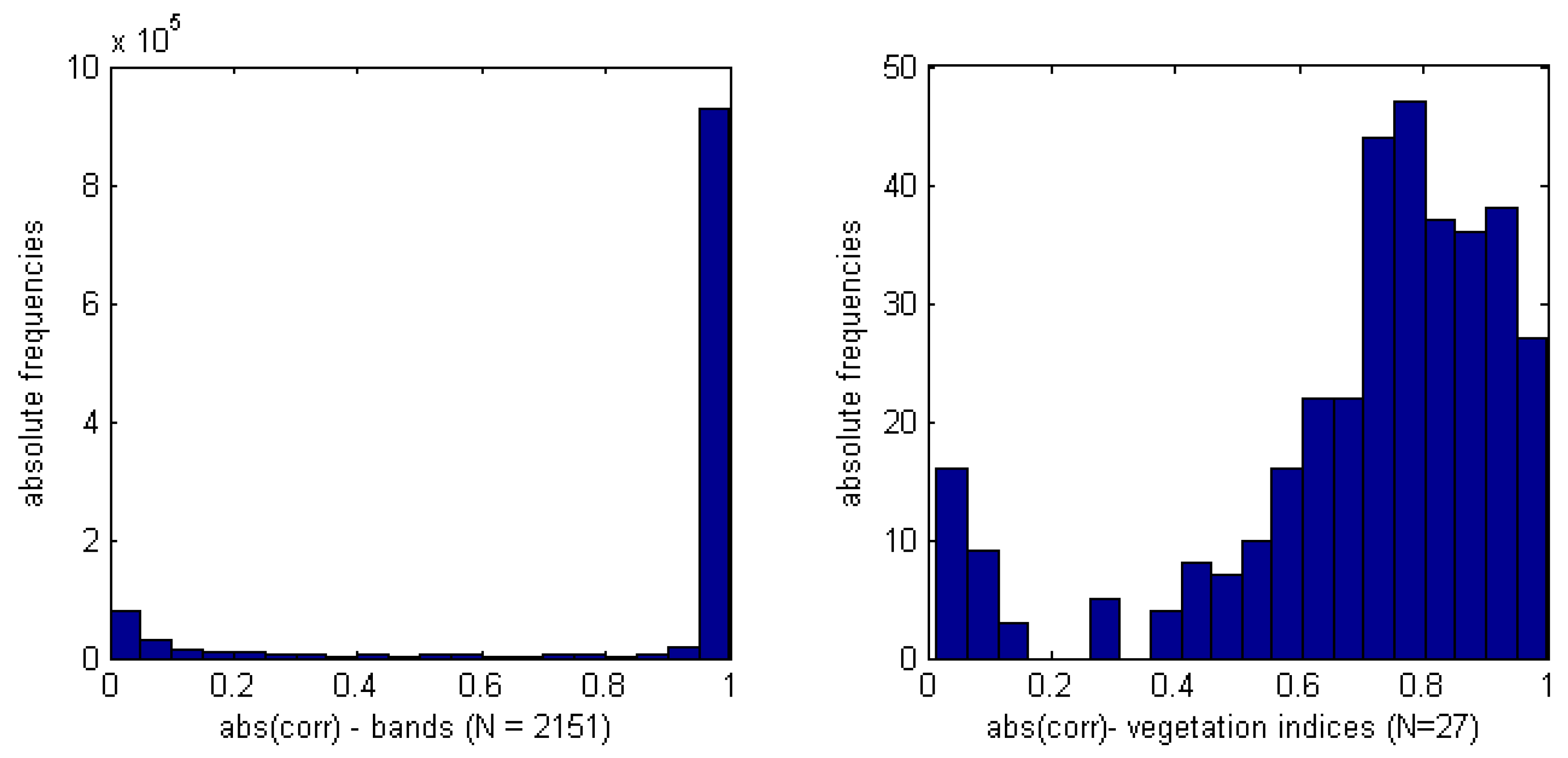
3.2. Dimensionality of the Spectral Data

The spectral reflectance properties presented in Figure 2 also illustrate—while containing some information on LAI and WC—that large spectral ranges vary similarly with time and in response to nutrient and water conditions [47]. Thus, many of the spectral bands are inadequate or redundant in their information content when retrieving plant and soil characteristics such as LAI, chlorophyll or leaf and soil water content [48]. In order to get estimates of the dimensionality of our experimental data set, which is an important guidance on the minimum band/index number necessary for any retrieval algorithm—both linear and non-linear, local and non-local methods are used in the following.

Linear Methods:

First, the complete spectral information with a number of 2,151 bands was used in a correlation analysis. Correlation coefficients of each band combination were calculated and the frequency distribution of their absolute values is presented in Figure 4 (left). It can be seen that the majority of values (~80%) are correlated to each other with absolute values greater than 0.95, indicating the redundancy in the information content. This is also highlighted by the results of a principal component analysis (PCA) over the whole set of bands, giving a first principal component (PC) with a loading of 99.4% and a second and third PC explaining no more than 0.38% and 0.21% of total variance, respectively (without figure).

Analyzing the correlation between selected spectral indices (see Table 1), it can be seen, that the proportion of pairs with correlation showing absolute values close to 1 is reduced, however the PCA analysis (without figure) shows an even higher loading of the first PC (99.99%). The correlation and the PCA-analysis for both, the individual spectral bands and the pre-selected spectral indices, suggest only a very low number of variables (here 1–3, dependent on the threshold value) needed to represent the spectral database information. This, however, only holds as long as there is no significant non-linearity present in the data that is not implicitly included by the use of complex spectral indices and that cannot be recovered by linear methods.

Figure 4. Histogram of the absolute values of pairwise correlation between individual bands (left) and vegetation indices (right) that are listed in Table 1. N indicates the number of spectral bands or vegetation indices considered. The total number of pairs can be calculated as N * (N − 1) /2.

Figure 4. Histogram of the absolute values of pairwise correlation between individual bands (left) and vegetation indices (right) that are listed in Table 1. N indicates the number of spectral bands or vegetation indices considered. The total number of pairs can be calculated as N * (N − 1) /2.

Non-linear Methods:

In contrast to the traditional linear techniques, nonlinear methods have the ability to deal with complex nonlinear data. Previous studies have shown that nonlinear techniques outperform their linear counterparts on complex artificial tasks. Examples are for instance the Swiss Roll dataset comprising a set of points that lie on a spiral-like two-dimensional manifold within a three-dimensional space [49,50]. These methods aim at finding the intrinsic dimensionality (d) of a data set, being the minimum number of parameters that is necessary in order to account for all information contained within.

Techniques for intrinsic dimensionality estimation can be subdivided into two main groups: (1) estimators based on the analysis of local properties of the data and (2) estimators based on the analysis of global properties of the data. Local methods used in this analysis comprise the correlation dimension estimator (CorrDim), the nearest neighbor dimension estimator (NNDim), and the maximum likelihood estimator (MaxLike). Global estimators additional to the PCA considered in this analysis are the packing number estimator (PackNum), and the geodesic minimum spanning tree estimator (GMST). These methods are briefly introduced in the Appendix, but readers are referred to the “Matlab Toolbox for Dimensionality Reduction drtoolbox” [51,52,53], for a more comprehensive discussion and comparison.

Table 3 compares these different methods for both the complete spectral dataset including all spectral bands and the dataset given by the spectral indices listed in Table 1. The results show similar values when comparing the estimated intrinsic dimensionalities for the two data sets, suggesting that the much smaller (N = 28 vs. N = 2151) set of indices might well be able to represent the entire information content of the original dataset of all spectral bands. Comparing d estimations from different techniques, they show some more pronounced deviations indicating the different foci of the methods with respect to the non-linear characteristics of the data. However, the estimated intrinsic dimensionality of both datasets ranges around 3–6 (PCA, GMST) and does not exceed a value of 8 (MAXLike).

Table 3. Estimated intrinsic dimensionalities (d) of the complete spectral dataset including all spectral bands and of the dataset given by the pre-selected spectral indices. (CorrDim–correlation dimension estimator, NNDim–nearest neighbor dimension estimator, MaxLike–maximum likelihood estimator, PackNum–packing number estimator, GMST–geodesic minimum spanning tree estimator, PCA–principal component analysis).

Intrinsic dimensionality d of the datasets
Methods/Dataset	all spectral bands (N = 2,151)	spectral indices (N = 28)
CorrDim	1.03	1.58
NNDim	0.18	0.28
MaxLike	8.08	4.82
PackNum	0.00	0.00
GMST	5.96	3.69
PCA*	4.00	3.00

* PCA has been included for comparison. d was derived by the number of PC with a minimum value of 0.25% for explaining total variance.

Table 3. Estimated intrinsic dimensionalities (d) of the complete spectral dataset including all spectral bands and of the dataset given by the pre-selected spectral indices. (CorrDim–correlation dimension estimator, NNDim–nearest neighbor dimension estimator, MaxLike–maximum likelihood estimator, PackNum–packing number estimator, GMST–geodesic minimum spanning tree estimator, PCA–principal component analysis).

Intrinsic dimensionality d of the datasets
Methods/Dataset	all spectral bands (N = 2,151)	spectral indices (N = 28)
CorrDim	1.03	1.58
NNDim	0.18	0.28
MaxLike	8.08	4.82
PackNum	0.00	0.00
GMST	5.96	3.69
PCA*	4.00	3.00

* PCA has been included for comparison. d was derived by the number of PC with a minimum value of 0.25% for explaining total variance.

These values give some guidance on the maximum number of SI’s as independent variable that will be needed in any type of regression or non-linear analysis.

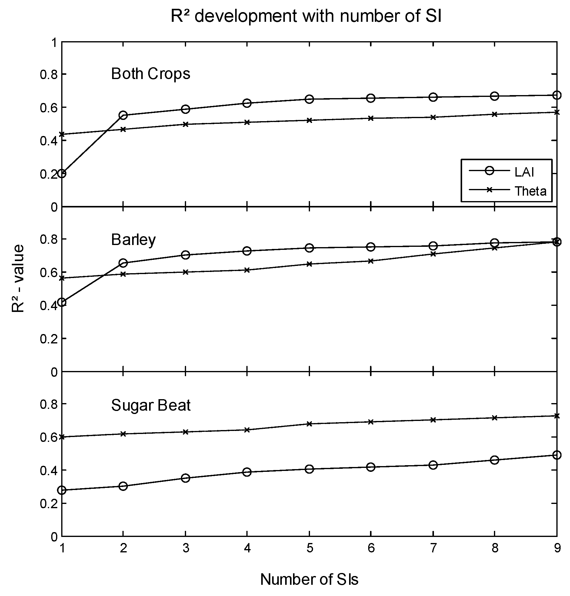
3.3. Retrieval of LAI and Soil Moisture by Linear Regression

The intrinsic dimensionality estimation as described in the previous section, suggest that most of the information content of the original spectral dataset can be well described by a set of 28 SI’s (Table 1). We therefore restrict any further analysis to this reduced data set. In a first step, the simple linear dependencies between LAI and soil WC and single SI’s are investigated. Standard linear regression was applied to extract the single SI with the maximum explanatory potential. Calculations were done for three variants: (1) using both crop types in one dataset and (2, 3) treating each crop species spring barley (2) and sugar beet (3) separately. Table 4 lists the coefficients of determination (R²) when predicting LAI and WC from a single SI for the three variants (1–3), as described above. Also given for each of the variants are the SI’s (according to Table 1) for which the maximum R² is achieved.

The results in Table 4 present a clear pattern: First, the R² values are relatively low in general with predictions being generally better for WC compared to LAI (maximum R² of 0.60 vs. 0.42) indicating that a single spectral index will not be sufficient to describe plant/soil variables over the range of conditions presented here by the individual nutrients and water treatments. Second, simple linear regression shows a better performance for both LAI and WC when applied to individual crop types rather than treating crops in a common application. In practice, this would mean that knowing crop species beforehand will significantly improve such retrieval, but will make the application of land use classification schemes necessary beforehand, thereby introducing potential misclassification error. The results from simple linear regressions (Table 4) as well as intrinsic dimensionality analysis of the spectral dataset suggest that multiple explanatory variables (3–4) should be able to more adequately explain the dynamic dependencies of WC, LAI and the vegetation spectral responses (SI’s).

Table 4. Coefficients of determination (R²) and root mean square error (rmse, in brackets) of simple univariate and multiple (three-fold) linear regressions between LAI/WC and pre-selected SI’s (see Table 1). Values listed are the maximum R² values and the corresponding root mean square error (rmse) when varying through all 28 indices for univariate linear regression and through all combinations of SI’s (one from each of the three functional groups, see Table 1) for multiple linear regression. This analysis has been performed using data for “both crops” (Spring Barley and Sugar Beet) together as well as separately (“only barley” and “only sugar”). The columns “SI” refers to the spectral index (see Table 1) achieving the best fit.

		Univariate Linear Regression		Multivariate Linear Regression (3 variables)
		R2 (rmse)	SI	R2 (rmse)	SI
WC [Vol.%]	both crops	0.43 (8.45)	MSI	0.49 (8.01)	RG, PSRI, MSI
	only barley	0.57 (7.14)	NWI_2	0.65 (6.43)	mNDVI_705, PRI, NWI_1
	only sugar	0.60 (7.32)	NDVI_a	0.65 (6.82)	RG, PSRI, MSI
LAI [m²m−2]	both crops	0.20 (1.40)	mSR_705	0.57 (1.03)	GNDVI, PRI, NDWI_2130
	only barley	0.42 (1.40)	GNDVI	0.67 (1.06)	GNDVI, PRI, NDWI_2130
	only sugar	0.27 (0.55)	MSR	0.33 (0.53)	RNDVI, PSRI, NWI_2

Table 4. Coefficients of determination (R²) and root mean square error (rmse, in brackets) of simple univariate and multiple (three-fold) linear regressions between LAI/WC and pre-selected SI’s (see Table 1). Values listed are the maximum R² values and the corresponding root mean square error (rmse) when varying through all 28 indices for univariate linear regression and through all combinations of SI’s (one from each of the three functional groups, see Table 1) for multiple linear regression. This analysis has been performed using data for “both crops” (Spring Barley and Sugar Beet) together as well as separately (“only barley” and “only sugar”). The columns “SI” refers to the spectral index (see Table 1) achieving the best fit.

		Univariate Linear Regression		Multivariate Linear Regression (3 variables)
		R2 (rmse)	SI	R2 (rmse)	SI
WC [Vol.%]	both crops	0.43 (8.45)	MSI	0.49 (8.01)	RG, PSRI, MSI
	only barley	0.57 (7.14)	NWI_2	0.65 (6.43)	mNDVI_705, PRI, NWI_1
	only sugar	0.60 (7.32)	NDVI_a	0.65 (6.82)	RG, PSRI, MSI
LAI [m²m−2]	both crops	0.20 (1.40)	mSR_705	0.57 (1.03)	GNDVI, PRI, NDWI_2130
	only barley	0.42 (1.40)	GNDVI	0.67 (1.06)	GNDVI, PRI, NDWI_2130
	only sugar	0.27 (0.55)	MSR	0.33 (0.53)	RNDVI, PSRI, NWI_2

In a next step, we therefore tested multiple linear regression using three explanatory SI’s—one from each functional group (see Table 1)—leading to a scenario of 560 possible combinations of three-parameter explanatory inputs. Calculations were done in a similar way using three variants (1) for the entire dataset incorporating both crops together and for each species separately: Spring Barley (2) and Sugar Beet (3). Results are shown in Table 4 (right), demonstrating a significant improvement in the retrieval of WC and LAI from a combination of SI’s for both the calculated R²-values as well as rmse. Interestingly, in four of the six applications, the SI’s that produced the best fit within the univariate regression analysis was not among the best combination of SI’s in the multiple regression approach, indicating that some of the individual SI’s might be better able to represented the combined plant response to water and nutrient stress, but a combination of each multiple SI’s are more selective to a certain aspect of plant stress response and perform better. In particular the retrieval of LAI (for both crops) has gained drastically from inclusion of additional SI’s confirming findings of e.g., [19] that LAI is not only influences by leaf chlorophyll concentration but also by other biochemical and crop/leaf structural factors that are possibly reflected in other SI’s.

While the results from dimensionality analysis suggested the use of 3–4 independent variable SI’s best representing the spectral information, we have investigated the consideration of further SI’s into the modeling procedure as shown in Figure 5. While considerable improvements in the prediction of LAI is achieved by an increase to three variables, only small increases in the model performance are observed by including additional SI’s as explanatory variables. For the WC retrieval, already one SI achieves relatively high R²—values that only slightly improved by adding further SI’s.

The overall performance of the multiple-(3-SI)-regression-retrieval approach with R²-values of 0.65 for WC (both crops), and 0.67 and 0.33 for LAI (barley and sugar beet, respectively) compare very much to the upper limit of results that have been summarized by [19] showing a range of 0.05–0.66 for the retrieval of LAI. However, it needs to be considered, that our experiments have been performed under local, partly idealized glasshouse conditions, with direct control on illumination conditions and without the disturbance of atmospheric effects.

Figure 5. R² improvement within multiple linear regression analysis due to increase of explanatory variables for LAI (continuous line) and theta (discontinuous line) for both crops species together (top), (2) for barley (middle), and (3) for sugar beet (bottom).

Figure 5. R² improvement within multiple linear regression analysis due to increase of explanatory variables for LAI (continuous line) and theta (discontinuous line) for both crops species together (top), (2) for barley (middle), and (3) for sugar beet (bottom).

3.4. Retrieval of LAI and Soil Moisture by Non-Linear Regression Trees

In addition to the multiple-linear regression approach, we have investigated the possible improvement and benefit of using non-linear techniques in the retrieval algorithm. A large variety of different techniques have been developed over the past decades, many of them emerging from the area of artificial intelligence, data mining and machine learning. Among those neuronal networks [54], fuzzy rules based approaches [55], support vector machines [56], random trees [57] and classification and regression trees (CART) [58] are the most popular.

The CART method was chosen here as it represents a simple, comprehensible, easily to implement and widely used method. It is a nonparametric modeling approach that can describe the responses of a dependent from a set of independent variables. In our application, CART recursively partition the set of SI’s to find increasingly homogeneous subsets based on SI’s splitting criteria using variance minimizing algorithms. The (dependent) LAI and WC data are partitioned into a series of descending left and right child nodes derived from parent nodes. Once the partitioning has ceased, the child nodes are designated as terminal nodes. For CART calibration, a cost function is defined as the product of the estimated probability of a node times the cost of a node, that is the average squared error over the observations in that node, summed over all terminal nodes [58]. The “optimal” size of the tree has been extracted using 10-fold cross-validation and choosing the smallest tree that is within one standard error of the minimum-cost sub-tree. As CART, as well as all the other non-linear techniques mentioned above, show the ability to “overfit” the available data, we have compared multiple-linear regression (as presented in Section 3.3) and CART in a cross-validation framework using a leave-one-out strategy.

Results shown in Table 5 using the combination of SI’s achieving the best results in the multiple-linear-regression analysis presented before (Table 4) clearly demonstrate the difficulties of using non-linear techniques. Using the standard settings of the CART tree building procedure, only the retrieval of LAI for both crops shows superior results to multiple-linear regression, while “fine-tuning” of individual settings in the tree-building has been shown to improve the validation results for one of the dependent variable and crop combinations, the decrease at the same time for the others.

Table 5. Coefficients of determination (R²) and root mean square errors (rmse) for multiple linear regression and CART between LAI and WC using the best combinations of pre-selected SI’s from the analysis in Section 3.3 within a cross-validation (leave-one-out) framework. Results are representing cross-validation results for both crops (Spring Barley and Sugar Beet) together and separately for each one.

		Mulitple Linear Regression	CART
		R2 (rmse)	R2 (rmse)
WC [Vol.%]	both crops	0.48 (8.08)	0.42 (8.59)
	only barley	0.63 (6.59)	0.43 (8.25)
	only sugar	0.64 (6.94)	0.61 (7.17)
LAI [m²m−2]	both crops	0.55 (1.05)	0.59 (1.01)
	only barley	0.65 (1.08)	0.58 (1.20)
	only sugar	0.30 (0.54)	0.18 (0.59)

Table 5. Coefficients of determination (R²) and root mean square errors (rmse) for multiple linear regression and CART between LAI and WC using the best combinations of pre-selected SI’s from the analysis in Section 3.3 within a cross-validation (leave-one-out) framework. Results are representing cross-validation results for both crops (Spring Barley and Sugar Beet) together and separately for each one.

		Mulitple Linear Regression	CART
		R2 (rmse)	R2 (rmse)
WC [Vol.%]	both crops	0.48 (8.08)	0.42 (8.59)
	only barley	0.63 (6.59)	0.43 (8.25)
	only sugar	0.64 (6.94)	0.61 (7.17)
LAI [m²m−2]	both crops	0.55 (1.05)	0.59 (1.01)
	only barley	0.65 (1.08)	0.58 (1.20)
	only sugar	0.30 (0.54)	0.18 (0.59)

While we do not want to generalize these finding to all other non-linear techniques listed above, we here want state that at least using the CART approach for the retrieval of LAI and WC for our experimental data did not show the potential for any improvement in the retrieval process. In consequence, this also means that most of the non-linearity that might be inherent in the LAI/WC to spectral reflectance dependency is already “included” in the non-linear combination of individual and selective narrow spectral bands of the SI’s.

4. Summary and Conclusions

Time series of hyper-spectral reflectance data (400–2,500 nm) for two crop species—sugar beet and spring barley—over a vegetation period clearly demonstrated a significant response of plant reflectance characteristics to variations in WC and nutrient conditions. Based on these findings, we investigated the potential of retrieving plant LAI and soil WC from spectral reflectance data. First, the full range of spectral bands (N = 2151), as well as a reduced spectral data-base consisting of 28 spectral indices extracted from literature review (see Table 1; N = 28), have been analyzed for their information in a system analysis sense. Using linear and non-linear techniques, the intrinsic dimensionality of both datasets suggested a number of 3–4 but not more than 8 bands/indices to fully represent the information contained in the spectral data. Results also suggest, that the full band information is well represented by the set of 28 SI’s that have been divided into three functional groups: (i) greenness/biomass/vegetation structure, (ii) pigment or light use efficiency, and (iii) water related indices (see Table 1).

Restricting the further analysis to the use of the set of SI’s, we subsequently analyzed the potential for LAI and WC retrieval from the SI’s using single and multiple linear regression. It was shown that including three indices in the retrieval algorithm—one index from each functional group—could significantly improve the results. In general, the retrieval of LAI and WC was significantly higher when only considering single species. R² values range from 0.65 for WC retrieval for both sugar beet and spring barley when treated separately, to 0.67 and 0.33 for LAI retrieval. These results are very much in line with a summary statistics of LAI retrieval results reviewed by [19] given values in the range of 0.05–0.66, however we have to consider that here we have been working under an almost ideal glasshouse situation with cultivated plants under optimal and controlled irrigation, fertilization and illumination conditions and were also able to achieve constant light source sensor configuration thereby avoiding bidirectional effects.

While the results achieved are promising, we still need to extend our analysis considering the following aspects: While the best retrieval results have been achieved considering only single crop species, this would require the application of classification schemes beforehand when applying glasshouse calibrated algorithms to “real world” field conditions. This is currently under investigation using field spectral measurements at selected experimental test plot of the Bad Lauchstädt long-term fertilization experiment and will be presented in near future.

The potential of non-linear retrieval algorithms needs to be extended to a more thorough analysis considering a larger variety of methods in addition to the CART approach presented here. However, first results presented here within a cross-validation framework suggest that most of the non-linearity in the LAI/WC to spectral reflectance relationship is already covered by the non-linearity of the SI’s applied, but needs to be further tested. Our aim in publishing the here presented data set to the remote sensing community will hopefully support this requirement.

While our analysis has mainly built on the use of SI’s, at least for the retrieval of LAI, the inversion of a leaf/canopy reflectance model such as PROSPECT/SAIL [36,46,59] might have the potential to improve the results, but again while being beyond the scope of this paper, this aspect needs to be investigated in more detail and is part of our current research activities that will certainly be presented in the near future.

References

1. Albertson, J.D.; Katul, G.G.; Wiberg, P. Relative importance of local and regional controls on coupled water, carbon, and energy fluxes. Adv. Water Resour. 2001, 24, 1103–1118. [Google Scholar] [CrossRef]
2. Schmugge, T.J.; Kustas, W.P.; Ritchie, J.C.; Jackson, T.J.; Rango, A. Remote sensing in hydrology. Adv. Water Resour. 2002, 25, 1367–1385. [Google Scholar] [CrossRef]
3. Asner, G.P. Biophysical and biochemical sources of variability in canopy reflectance. Remote Sens. Environ. 1998, 64, 234–253. [Google Scholar] [CrossRef]
4. Asner, G.P.; Wessman, C.A.; Schimel, D.S.; Archer, S. Variability in leaf and litter optical properties: Implications for BRDF model inversions using AVHRR, MODIS, and MISR. Remote Sens. Environ. 1998, 63, 243–257. [Google Scholar] [CrossRef]
5. Goward, S.N.; Cruickshanks, G.D.; Hope, A.S. Observed relation between thermal emission and reflected spectral radiance of a complex vegetated landscape. Remote Sens. Environ. 1985, 18, 137–146. [Google Scholar] [CrossRef]
6. Penuelas, J.; Filella, I.; Biel, C.; Serrano, L.; Save, R. The reflectance at the 950–970 nm region as an indicator of plant water status. Int. J. Remote Sens. 1993, 14, 1887–1905. [Google Scholar] [CrossRef]
7. Penuelas, J.; Filella, I.; Gamon, J.A. Assessment of photosynthetic radiation-use efficiency with spectral reflectance. New Phytol. 1995, 131, 291–296. [Google Scholar] [CrossRef]
8. Yuan, W.P.; Liu, S.; Zhou, G.S.; Zhou, G.Y.; Tieszen, L.L.; Baldocchi, D.; Bernhofer, C.; Gholz, H.; Goldstein, A.H.; Goulden, M.L.; Hollinger, D.Y.; Hu, Y.; Law, B.E.; Stoy, P.C.; Vesala, T.; Wofsy, S.C. Other AmeriFlux Collaborators Deriving a light use efficiency model from eddy covariance flux data for predicting daily gross primary production across biomes. Agric. For. Meteorol. 2007, 143, 189–207. [Google Scholar] [CrossRef]
9. Deering, D.W.; Rouse, J.W.; Haas, R.H.; Schell, J.A. Measuring “forage production” of grazing units from Landsat MSS data. In Proceeding of International Symposium on Remote Sensing of Environment, Ann Arbor, CA, USA, October 1975; pp. 1169–1178.
10. Rouse, J.W.; Haas, R.H.; Schell, J.A.; Deering, D.W. Monitoring vegetation systems in the Great Plains with ERTS. In Proceeding of Goddard Space Flight Center 3rd ERTS-1 Symposium, Washinton, DC, USA; 1974. No. SP-351 I. pp. 309–317. [Google Scholar]
11. Gamon, J.A.; Field, C.B.; Bilger, W.; Bjorkman, O.; Fredeen, A.L.; Penuelas, J. Remote sensing of the xanthophyll cycle and chlorophyll fluorescence in sunflower leaves and canopies. Oecologia 1990, 85, 1–7. [Google Scholar] [CrossRef]
12. Gamon, J.A.; Penuelas, J.; Field, C.B. A narrow-waveband spectral index that tracks diurnal changes in photosynthetic efficiency. Remote Sens. Environ. 1992, 41, 35–44. [Google Scholar] [CrossRef]
13. Penuelas, J.; Llusia, J.; Pinol, J.; Filella, I. Photochemical reflectance index and leaf photosynthetic radiation-use-efficiency assessment in Mediterranean trees. Int. J. Remote Sens. 1997, 18, 2863–2868. [Google Scholar] [CrossRef]
14. Penuelas, J.; Gamon, J.A.; Fredeen, A.L.; Merino, J.; Field, C.B. Reflectance indexes associated with physiological changes in nitrogen-limited and water-limited sunflower leaves. Remote Sens. Environ. 1994, 48, 135–146. [Google Scholar] [CrossRef]
15. Gao, B.C. NDWI—a normalized difference water index for remote sensing of vegetation liquid water from space. Remote Sens. Environ. 1996, 58, 257–266. [Google Scholar] [CrossRef]
16. Hunt, E.R.; Rock, B.N. Detection of changes in leaf water-content using near-infrared and middle-infrared reflectances. Remote Sens. Environ. 1989, 30, 43–54. [Google Scholar]
17. Penuelas, J.; Filella, I. Visible and near-infrared reflectance techniques for diagnosing plant physiological status. Trends Plant Sci. 1998, 3, 151–156. [Google Scholar] [CrossRef]
18. Chen, D.Y.; Huang, J.F.; Jackson, T.J. Vegetation water content estimation for corn and soybeans using spectral indices derived from MODIS near- and short-wave infrared bands. Remote Sens. Environ. 2005, 98, 225–236. [Google Scholar] [CrossRef]
19. Haboudane, D.; Miller, J.R.; Pattey, E.; Zarco-Tejada, P.J.; Strachan, I.B. Hyperspectral vegetation indices and novel algorithms for predicting green LAI of crop canopies: Modeling and validation in the context of precision agriculture. Remote Sens. Environ. 2004, 90, 337–352. [Google Scholar] [CrossRef]
20. Gitelson, A.; Merzlyak, M.N. Quantitative estimation of chlorophyll-a using reflectance spectra experiments with autumn chestnut and maple leaves. J. Photochem. Photobiol. B 1994, 22, 247–252. [Google Scholar] [CrossRef]
21. Sims, D.A.; Gamon, J.A. Relationships between leaf pigment content and spectral reflectance across a wide range of species, leaf structures and developmental stages. Remote Sens. Environ. 2002, 81, 337–354. [Google Scholar] [CrossRef]
22. Datt, B. A new reflectance index for remote sensing of chlorophyll content in higher plants: Tests using Eucalyptus leaves. J. Plant Physiol. 1999, 154, 30–36. [Google Scholar] [CrossRef]
23. Babar, M.A.; Reynolds, M.P.; van Ginkel, M.; Klatt, A.R.; Raun, W.R.; Stone, M.L. Spectral reflectance indices as a potential indirect selection criteria for wheat yield under irrigation. Crop Sci. 2006, 46, 578–588. [Google Scholar] [CrossRef]
24. Gitelson, A.A.; Kaufman, Y.J.; Merzlyak, M.N. Use of a green channel in remote sensing of global vegetation from EOS-MODIS. Remote Sens. Environ. 1996, 58, 289–298. [Google Scholar] [CrossRef]
25. Chen, J.M. Evaluation of vegetation indices and a modified simple ratio for boreal applications. Can. J. Rem. Sens. 1996, 22, 229–242. [Google Scholar] [CrossRef]
26. Aparicio, N.; Villegas, D.; Casadesus, J.; Araus, J.L.; Royo, C. Spectral vegetation indices as nondestructive tools for determining durum wheat yield. Agronom. J. 2000, 92, 83–91. [Google Scholar] [CrossRef]
27. Merzlyak, M.N.; Gitelson, A.A.; Chivkunova, O.B.; Rakitin, V.Y. Non-destructive optical detection of pigment changes during leaf senescence and fruit ripening. Physiol. Plant. 1999, 106, 135–141. [Google Scholar] [CrossRef]
28. Penuelas, J.; Baret, F.; Filella, I. Semiempirical indexes to assess carotenoids chlorophyll-a ratio from leaf spectral reflectance. Photosynthetica 1995, 31, 221–230. [Google Scholar]
29. Penuelas, J.; Pinol, J.; Ogaya, R.; Filella, I. Estimation of plant water concentration by the reflectance water index WI (R900/R970). Int. J. Remote Sens. 1997, 18, 2869–2875. [Google Scholar] [CrossRef]
30. Pu, R.; Ge, S.; Kelly, N.M.; Gong, P. Spectral absorption features as indicators of water status in coast live oak (Quercus agrifolia) leaves. Int. J. Remote Sens. 2003, 24, 1799–1810. [Google Scholar] [CrossRef]
31. Ceccato, P.; Flasse, S.; Tarantola, S.; Jacquemoud, S.; Grégoire, J.-M. Detecting vegetation leaf water content using reflectance in the optical domain. Remote Sens. Environ. 2001, 77, 22–33. [Google Scholar] [CrossRef]
32. Hardisky, M.A.; Klemas, V.; Smart, R.M. The influence of soil-salinity, growth form, and leaf moisture on the spectral radiance of Spartina-Alterniflora canopies. Photogramm. Eng. Rem. Sens. 1983, 49, 77–83. [Google Scholar]
33. Jackson, T.J.; Chen, D.Y.; Cosh, M.; Li, F.Q.; Anderson, M.; Walthall, C.; Doriaswamy, P.; Hunt, E.R. Vegetation water content mapping using Landsat data derived normalized difference water index for corn and soybeans. Remote Sens. Environ. 2004, 92, 475–482. [Google Scholar] [CrossRef]
34. Bonan, G.B. Importance of leaf area index and forest type when estimating photosynthesis in boreal forests. Remote Sens. Environ. 1993, 43, 303–314. [Google Scholar] [CrossRef]
35. Bonan, G.B. Land-Atmosphere interactions for climate system Models: Coupling biophysical, biogeochemical, and ecosystem dynamical processes. Remote Sens. Environ. 1995, 51, 57–73. [Google Scholar] [CrossRef]
36. Jacquemoud, S.; Verhoef, W.; Baret, F.; Bacour, C.; Zarco-Tejada, P.J.; Asner, G.P.; François, C.; Ustin, S.L. PROSPECT+SAIL models: A review of use for vegetation characterization. Remote Sens. Environ. 2009, 113, S56–S66. [Google Scholar] [CrossRef]
37. Panciera, R.; Walker, J.P.; Kalma, J.D.; Kim, E.J.; Saleh, K.; Wigneron, J.-P. Evaluation of the SMOS L-MEB passive microwave soil moisture retrieval algorithm. Remote Sens. Environ. 2009, 113, 435–444. [Google Scholar] [CrossRef]
38. Saleh, K.; Kerr, Y.H.; Richaume, P.; Escorihuela, M.J.; Panciera, R.; Delwart, S.; Boulet, G.; Maisongrande, P.; Walker, J.P.; Wursteisen, P.; Wigneron, J.P. Soil moisture retrievals at L-band using a two-step inversion approach (COSMOS/NAFE’05 Experiment). Remote Sens. Environ. 2009, 113, 1304–1312. [Google Scholar] [CrossRef] [Green Version]
39. Grant, J.P.; de Griend, A.A.V.; Wigneron, J.P.; Saleh, K.; Panciera, R.; Walker, J.P. Influence of forest cover fraction on L-band soil moisture retrievals from heterogeneous pixels using multi-angular observations. Remote Sens. Environ. 2010, 114, 1026–1037. [Google Scholar] [CrossRef]
40. Jacquemoud, S.; Baret, F.; Andrieu, B.; Danson, F.M.; Jaggard, K. Extraction of vegetation biophysical parameters by inversion of the PROSPECT + SAIL models on sugar beet canopy reflectance data. Application to TM and AVIRIS sensors. Remote Sens. Environ. 1995, 52, 163–172. [Google Scholar] [CrossRef]
41. Leifeld, J.; Franko, U.; Schulz, E. Thermal stability responses of soil organic matter to long-term fertilization practices. Biogeosci. 2006, 3, 371–374. [Google Scholar] [CrossRef]
42. Schaecke, W.; Tanneberg, H.; Schilling, G. Behavior of heavy metals from sewage sludge in a Chernozem of the dry belt in Saxony-Anhalt/Germany. J. Plant Nutr. Soil Sci. 2002, 165, 609–617. [Google Scholar] [CrossRef]
43. Embacher, A.; Zsolnay, A.; Gattinger, J.; Munch, J.C. The dynamics of water extractable organic matter (WEOM) in common arable topsoils: I. Quantity, quality and function over a three year period. Geoderma 2007, 139, 11–22. [Google Scholar] [CrossRef]
44. Castro-Esau, K.L.; Sanchez-Azofeifa, G.A.; Rivard, B. Comparison of spectral indices obtained using multiple spectroradiometers. Remote Sens. Environ. 2006, 103, 276–288. [Google Scholar] [CrossRef]
45. Jacquemoud, S.; Baret, F.; Hanocq, J.F. Modeling spectral and bidirectional soil reflectance. Remote Sens. Environ. 1993, 41, 123–132. [Google Scholar] [CrossRef]
46. Jacquemoud, S.; Baret, F. PROSPECT: A model of leaf optical properties spectra. Remote Sens. Environ. 1990, 34, 75–91. [Google Scholar] [CrossRef]
47. Grossman, Y.L.; Ustin, S.L.; Jacquemoud, S.; Sanderson, E.W.; Schmuck, G.; Verdebout, J. Critique of stepwise multiple linear regression for the extraction of leaf biochemistry information from leaf reflectance data. Remote Sens. Environ. 1996, 56, 182–193. [Google Scholar] [CrossRef]
48. Thenkabail, P.S.; Enclona, E.A.; Ashton, M.S.; Van der Meer, B. Accuracy assessments of hyperspectral waveband performance for vegetation analysis applications. Remote Sens. Environ. 2004, 91, 354–376. [Google Scholar] [CrossRef]
49. Tenenbaum, J.B. Mapping a manifold of perceptual observations; Massachusetts Institute of Technology: Cambrige, MA, USA, 1998. [Google Scholar]
50. Tenenbaum, J.B.; de Silva, V.; Langford, J.C. A global geometric framework for nonlinear dimensionality reduction. Science 2000, 290, 2319–2323. [Google Scholar] [CrossRef] [PubMed]
51. Van der Maaten, L.J.P. An Introduction to Dimensionality Reduction Using Matlab; TiCC, Tilburg University: Tilburg, The Netherlands, 2007. [Google Scholar]
52. Van der Maaten, L.J.P. Drtoolbox—Matlab Toolbox for Dimensionality Reduction, 0.7b; TiCC, Tilburg University: Tilburg, The Netherlands, 2008. [Google Scholar]
53. Van der Maaten, L.J.P.; Postma, E.O.; Herik van den, H.J. Dimensionality Reduction: A Comparative Review; TiCC, Tilburg University: Tilburg, The Netherlands, 2008. [Google Scholar]
54. Kriesel, D. A Brief Introduction to Neural Networks. Available online: http://www.dkriesel.com/en/science/neural_networks (accessed on 10 May 2010).
55. Baldwin, J.F. Fuzzy logic and fuzzy reasoning. In Fuzzy Reasoning and Its Applications; Mamdani, E.H., Gaines, B.R., Eds.; Academic Press: London, UK, 1981. [Google Scholar]
56. Cristianini, N.; Shawe-Taylor, J. An Introduction to Support Vector Machines (and Other Kernel-Based Learning Methods); Cambridge University Press: Cambridge, UK, 2000. [Google Scholar]
57. Drmota, M. Random Trees: An Interplay between Combinatorics and Probability; Springer Wien New York: New York, NY, USA, 2009. [Google Scholar]
58. Breiman, L.; Friedman, J.H.; Olshen, R.A.; Stone, C.J. Classification and Regression Trees; Wadsworth, Inc.: Monterey, CA, USA, 1984. [Google Scholar]
59. Jacquemoud, S. Inversion of the Prospect+Sail canopy reflectance model from Aviris equivalent spectra theoretical study. Remote Sens. Environ. 1993, 44, 281–292. [Google Scholar] [CrossRef]