Channel and Floodplain Change Analysis over a 100-Year Period: Lower Yuba River, California

Abstract

Hydraulic gold mining in the Sierra Nevada, California (1853–1884) displaced ~1.1 billion m³ of sediment from upland placer gravels that were deposited along piedmont rivers below dams where floods can remobilize them. This study uses topographic and planimetric data from detailed 1906 topographic maps, 1999 photogrammetric data, and pre- and post-flood aerial photographs to document historic sediment erosion and deposition along the lower Yuba River due to individual floods at the reach scale. Differencing of 3 × 3-m topographic data indicates substantial changes in channel morphology and documents 12.6 × 10⁶ m³ of erosion and 5.8 × 10⁶ m³ of deposition in these reaches since 1906. Planimetric and volumetric measurements document spatial and temporal variations of channel enlargement and lateral migration. Over the last century, channels incised up to ~13 m into mining sediments, which dramatically decreased local flood frequencies and increased flood conveyance. These adjustments were punctuated by event-scale geomorphic changes that redistributed sediment and associated contaminants to downstream lowlands.

1. Introduction

Floodplains are formed by a complex interaction of fluvial processes. Their character and evolution depends upon stream power, sediment behavior, and channel features [1]. Floodplains have been extensively used for human activities like agriculture, settlement, and industry for millennia, and are vulnerable to morphologic changes to adjacent channels. Study of floodplain formation, stability, and the frequency of flooding is of utmost importance in the river sciences [2]. Changes in river courses and channel morphology alter the characteristics of floodplains, and may abandon floodplains as terraces. These changes often occur at a spatial scale that is ideal for study by remote sensing methods. Floodplain changes may be slow and progressive or rapid in the sense of geologic time, and may occur naturally or in response to human activities. This study examines a large river system that experienced rapid change as a consequence of massive sedimentation by hydraulic gold-mining activities between 1853 and 1884. While broad historical floodplains in the study area are now terraces abandoned by channel incision, they are located between high levees and are flooded on a decadal time scale. This study focuses on the recovery from 1906 to 1999 of the historical floodplain system, including terraces. The system has changed so substantially and quickly both horizontally and vertically that it is ideally suited for change-detection studies.

1.1. Using Remote Sensing for Floodplain Change Detection

Remote sensing technologies are increasingly being used to analyze fluvial landforms and processes [3]. Information on river morphology and changes over time is commonly needed for water resources planning and river management [4]. This information can be studied using recent and historical remotely sensed data [5]. Precise information on the quality, availability and capability of resources can be collected and analyzed by modern cartographic technologies utilizing satellite images, geographical information systems (GIS), global positioning systems (GPS) and light detection and ranging (LIDAR). Thus, satellite remote sensing and aerial photography can play an important role in generating information about river systems and their temporal changes through time. The basis of fluvial geomorphology is the analysis of river process and form, traditionally accomplished from field surveys and measuring sediment and hydrologic flows [6]. Aerial photographs, satellite images, and DEMs can be used to measure planimetric and volumetric changes within channels and analyze sediment fluxes over time [7,8].

Several studies have analyzed historic maps, aerial photographs, and other imagery to quantify channel and floodplain features and detect changes. Ham and Church [9] mapped channel features for five dates between 1952 and 1991, using GIS to analyze changes in erosion and deposition volumes and relate those volumetric changes to bed material transport and overbank sedimentation. Warburton et al. [10] studied the effect of both mining and flood phases on the temporal and spatial variability of a stream in northern England using aerial photographs and satellite images. Warner [11] measured gross channel changes for the Durance River in Southern France using topographic maps from 1890s and 1980s. Wellmeyer et al. [12] used a series of historical aerial photographs from 1938 to 1995 to study channel morphological changes and subsequent changes in potential for erosion downstream due to construction of an upstream dam. They were able to characterize rates of channel shifting and abandonment for each aerial photograph interval by delineating the area occupied by the channel each year and overlaying the images.

Technological advances in remotely-sensed topographic surveying technologies over the past three decades facilitate acquisition of topographic data in the fluvial environment with high spatial and temporal resolutions. Consequently, monitoring geomorphic changes and estimating fluvial sediment budgets through comparisons of repeat topographic surveys (e.g., DEM differencing) has become a feasible and affordable approach for both research purposes and long-term monitoring associated with fluvial systems [7,13,14]. This study utilizes remote sensing and GI-Science methods to measure and evaluate geomorphic changes and sediment budgets along the lower Yuba River in the Sacramento Valley, California, in terms of volumetric and surface-area changes that are attributable to erosion and deposition. However, this study does not compute sediment transport rates, which will be reserved for future study.

1.2. Background and Study Area

Floodplain sedimentation with alluvium derived from hydraulic gold mining in the Sierra Nevada of northeastern California is a major example of anthropogenic impacts on a fluvial system. Hydraulic mining displaced more than one billion m³ of sediment [15,17] as a by-product of gold extraction from placer gravels. Rapid delivery of hydraulic mining sediment (HMS) overwhelmed the transport capacity of rivers and caused channel aggradation from the mountains through the Sacramento Valley. The Yuba, Feather and Bear River basins were the main areas of concentration for hydraulic mining [16,17] in the Sierra Nevada. Over a period of 31 years of mining (1853–1884), the total volume of HMS production for the Yuba Basin was on the order of 523 × 10⁶ m³ [16,17]. Large deposits of HMS remain in the bed, banks, and terraces downstream of dams in the Sierra Nevada foothills and are subject to remobilization by floods [18]. As a result, substantial morphological changes, such as channel incision and migration, have occurred in the Yuba and Feather Rivers in response to floods. A number of river management and flood-control strategies such as dams, levees, channelization, and bank protection have been employed to control the inflow and reworking of mining sediment, which also resulted in substantial morphological changes in the system [18]. Remobilization of HMS stored along the lower Bear, Yuba, and Feather Rivers represents a substantial delivery of sediment to the modern channel system. The spatial and temporal distributions of this huge deposit and its potential redistribution or reworking by floods are poorly understood. Modern patterns of sedimentation downstream may affect flood conveyance in the lower Sacramento Valley [19]. At least eight major (peak discharge > 2,500 m³s⁻¹) floods (1907, 1909, 1955, 1964, 1970, 1986, 1997, 2005) evident from United States Geological Survey (USGS) stream gauge data have occurred in the lower Sacramento Valley since the turn of the 20th century.

The Sacramento Valley is the northern half of the Central Valley of California. The Yuba River is one of four large tributaries that flow out of the Sierra Nevada and ultimately deliver water and sediment to the Sacramento River (Figure 1). The Yuba River drains into the Feather River, which is the largest tributary of the Sacramento River. The lower Yuba River flows from Englebright Dam, through the Yuba Gold Fields over Daguerre Point Dam, to the Feather River at Marysville (Figure 2). Englebright Dam traps most sediment leaving the mountains and has arrested the delivery of reworked hydraulic mining sediment to the Valley since it was constructed in 1941 [15,20,21]. Most sediment transport in the lower Yuba River is produced from mining sediment stored downstream of Englebright, where the valley is wider, gradients decrease and much HMS was deposited. The Daguerre Point Reservoir has a low capacity and trap efficiency (it has been full of sediment since shortly after construction) and, therefore, has had a limited impact on sediment transport. This study focuses on the lower Yuba River below the dredged areas of the Yuba Gold Fields, where the river flows approximately 12 river km between levees and terraces to its confluence with the Feather River.

Figure 1. Map showing Yuba River within the watershed of the Feather River in Central Valley, California. The red box along the lower Yuba River shows the location of Figure 2.

Figure 1. Map showing Yuba River within the watershed of the Feather River in Central Valley, California. The red box along the lower Yuba River shows the location of Figure 2.

Two reach-scale study sites, Y3 and Y4, are presented here as the first of a larger set of sites being processed for detailed study (Figure 2). Sites Y3 and Y4 include high-amplitude meander bends, located downstream of the Yuba Gold Fields and upstream of Marysville, respectively. Both study reaches have flood-control levees set back several km from the channel, which were begun during the mining period and upgraded over a long period. The river is mostly a single-thread, gravel-bedded channel along this stretch with high terraces and banks consisting of historical mining sediment on both sides.

Figure 2. Lower Yuba River from Yuba Gold Fields (YGF) to the confluence with Feather River at Marysville (M). Y3 and Y4 are the study sites. The Yuba Gold Fields are an area where dredge mining occurred primarily after hydraulic mining ceased [22].

Figure 2. Lower Yuba River from Yuba Gold Fields (YGF) to the confluence with Feather River at Marysville (M). Y3 and Y4 are the study sites. The Yuba Gold Fields are an area where dredge mining occurred primarily after hydraulic mining ceased [22].

1.3. Relaxation from Channel and Floodplain Metamorphosis

This study is concerned primarily with the period from 1906 to 2006, for which detailed topographic data are available. However, the earlier period in the second half of the 19th century, when hydraulic mining resulted in rapid channel aggradation and floodplain metamorphism, is important for understanding the rates and character of change documented here. In the late 1800s, the lower Yuba channels filled with HMS so deeply and rapidly that channel avulsions were common and channels in this reach shifted from an anastomosed dual-channel pattern to braided and anastomosed patterns during the mining period and had begun to shift toward a single-thread pattern by 1906 [18]. Approximately 400 × 10⁶ m³ (38%) of the HMS produced in the northern Sierra Nevada was stored in piedmont deposits of the Yuba, Bear and lower Feather Rivers [16,17,18]. Pre-mining channels in the Sacramento Valley were described as having high, steep banks with dark, fertile soils on low terraces [18]. The rapid influx of HMS and human endeavors to control it caused extensive and prolonged channel changes to the Yuba River. The Yuba floodplains upstream of Marysville were the most extensively alluviated river reaches in the foothills or Valley. In the lower 12 km above the mouth of the Yuba River at Marysville, gradients decrease and floodplains broaden as Holocene alluvium overlaps onto Quaternary outwash terraces emanating from the Sierra Nevada. The pre-mining lower Yuba River was primarily a sinuous anastomosing channel system [18]. Mining sediment ultimately spread out across the lower Yuba floodplain causing multiple avulsions in the late 19th century. The first detailed topographic survey of the Yuba floodplain was performed in 1879 by the department of the State Engineer. Due to the high influx of sediment and frequent flooding by that time, the Yuba River was a multithread channel system that had shifted from its pre-mining position [18]. In fact, between 1861 and 1906, during the period of rapid aggradation, the channel occupied several positions distinct from its present location. Levees, dikes, and other engineering works were constructed to stabilize the channel, and by the turn of the 20th century, historical sediment deposits were largely bracketed by an extensive levee system [18]. Channel and floodplain changes that occurred subsequent to the rapid influx and cessation of HMS deliveries are the focus of this study.

2. Objectives

This study uses remote sensing change-detection techniques to examine spatial and temporal patterns of HMS redistribution at a centennial scale and to measure and evaluate the magnitude and processes of a major channel and floodplain metamorphosis. Most of the historical sediment initially stored on floodplains remains in storage [17] and some of it is subject to reworking by floods. These patterns of erosion and deposition have important practical implications because reworked sediment may impair flood conveyance in the Sacramento Valley flood control system and much of the mining sediment contains high concentrations of mercury [19]. Availability of early high-resolution topographic maps and more recent high resolution photogrammetric data provides an excellent opportunity to apply remote sensing methods to characterize channel metamorphosis in a rapidly changing channel system.

The specific objectives of this study are to calculate volumetric changes in sediment storage in channels and floodplains over the longer period from 1906 to 1999 and planimetric changes at a higher temporal resolution for seven periods bracketed by eight years for which spatial data were developed: 1906, 1947, 1958, 1967, 1975, 1986, 1999, and 2006. It is well understood from previous work that morphologic changes have been extreme over the extended period [18]. The 1906 to 1999 change analysis is performed to quantify volumes and identify specific locations and landform types associated with recovery from earlier changes. The hypothesis that morphologic changes during the early 20th century were greater than subsequent changes is tested with the planimetric data. In both cases (volumetric and planimetric), flood erosion and deposition are computed for each time period. At least eight major floods have occurred in the lower Sacramento Valley since the turn of the 20th century and the higher temporal resolution of the planimetric analysis allows change detection to be attributed to individual floods.

3. Methods

Spatial and temporal variations in channel dimensions, lateral migration, floodplain scour and fill, and associated volumes and areas of erosion and sedimentation were measured from historical maps and imagery. Two fundamental methods were used for change detection: DEM differencing and planimetric change analysis. The DEM differencing recorded volumetric changes in sediment storage at relatively high spatial resolutions; i.e., 3-D change surfaces were generated at 3 × 3 m spatial resolutions. Volumetric analysis was based on the delineation of four geomorphic features or landforms: modern perennial channels, emergent bars, terraces, and high-water channels. Modern perennial channels are defined as areas that lie below the low-flow stage in aerial photographs. Emergent bars are areas located up to 3 meters above the low-flow stage when aerial photographs were flown. Terraces are historical floodplains 3 to 6 meters above the active channel. High-water channels are ephemeral conduits for overbank flows during flood conditions (Figure 3).

Figure 3. Study sites Y3 and Y4. The background is a hillshade visualization derived from a DEM of 1999 photogrammetrically and SONAR-derived topographic data (PDTD [23,24,25]). White spots are missing data from photogrammetric analysis.

Figure 3. Study sites Y3 and Y4. The background is a hillshade visualization derived from a DEM of 1999 photogrammetrically and SONAR-derived topographic data (PDTD [23,24,25]). White spots are missing data from photogrammetric analysis.

3.1. Scope of Study

Two sites (~2–3 km in length) along the lower Yuba River below the Yuba Gold fields were studied (Figure 3). Sites Y3 and Y4 include bends along the Lower Yuba River that are characterized by incised channels with gravel bars and wide historical terraces with a high-water channel system. Each site contains all four of the geomorphic features discussed above. The northwest and southeast boundaries of the study areas terminate at flood-control levees in the distal floodplain. The Y4 site includes the U.S. Geological Survey stream-gauge site near Marysville (Station ID: 11421500). These two sites were chosen because they each exhibited a considerable amount of channel change during the period 1906 to 2006, and are representative of changes elsewhere in the fluvial system. Below the study area, river gradients are substantially lower and the gravel-sand transition in bed material occurs between Simpson Bridge and the Yuba-Feather confluence.

3.2. Data Preparation

Historical maps, aerial photographs, digital orthophoto quarter quads (DOQQs), SONAR and photogrammetrically derived topographic data (PDTD) were analyzed. Aerial photographs, orthophotos, and historic survey maps were used to measure planimetric changes and rates of channel migration for the lower Yuba Rivers. DEMs extracted from PDTD and historic topographic maps, were used to estimate the volumetric changes in sediment storage both in channel beds and floodplains. Pre- and post-flood aerial photographs were used for planimetric analysis.

3.2.1. 1906 CDC Topographic Maps and DEM Generation

A set of high-resolution topographic maps (Figure 4) produced by California Debris Commission (CDC) [26] was used to generate 1906 DEMs for the lower Yuba River. These maps contain bathymetric contours that show channel-bed elevations of the Yuba River. The CDC 1906 dataset comes in 13 large sheets, with six topographic map sheets and six sheets of channel cross-sections and a longitudinal profile. Each sheet was scanned in nine rectangular sections at 400 dpi using an A4 portable scanner at the map library at the University of California, Davis. Each section was merged manually into a complete sheet using Adobe Photoshop 7 and Macromedia Freehand 8 software. The merging of the sections was necessary as some individual sections do not have good GCP control owing to limited distinctive landscape features correlating to DOQQs and air photos. Merging was guided by matching the township-range survey points of the Public Land Survey System (PLSS) shown clearly on the maps. The merged sheets were georectified using section corners on the PLSS reference map. The average RMSE for rectification of five of these sheets is 5.47 m; relatively high owing to the merging of panels for each sheet. Vertical registration of the CDC (1906) Yuba River map sheets required an empirical fit of the data. The original CDC map was surveyed in the U.S.E.D datum as was printed on the first map sheet near Marysville:

“Elevations are expressed in feet and tenths and are referred to U.S.E.D. datum plane, which is 3.60 ft. below mean sea level, the datum plane of the U.S. Geological Survey, and are based on a benchmark of that survey at Oroville” [26].

An empirical test of the vertical registration was conducted by comparing the elevations of stable 1906 and 1999 (PDTD) surfaces outside of levees, along 8 cross sections generated from 1999 PDTD data and the 1906 CDC data. For example, cross section 19 is representative. Although it is slightly (~800 m) outside the study area, it is within the same CDC map sheet 2. Due to a relatively planar surface along this cross section, it was chosen to address the vertical datum registration. These comparisons show that the vertical datum of the 1906 DEM should be lowered by 1.2 meters (Figure 5). Such an empirical fitting method is suitable for the analysis of channel and floodplain morphological changes conducted here. Although it could be argued that some proportion of the 1.2 m vertical difference is real, owing to broad regional surface lowering by aquifer subsidence caused by groundwater mining and compaction of HMS, such broadly extensive differences are not the subject of this study, which is concerned with floodplain geomorphic adjustments and sediment reworking. The empirical fit of the successive DEMs based on relatively stable floodplain surfaces ensured that the volumetric difference in sediment budgets and morphological changes are not affected by sediment compaction, regional subsidence or geodetic registration error.

After the CDC (1906) [26] map data were horizontally and vertically registered, contour lines, including subaqueous bathymetry, from the 1906 maps were digitized in ArcGIS 9.2. DEMS at 3 × 3 m resolution were generated by a non-linear TIN interpolation using Erdas Imagine 9.2 for each of the two study sites from the digitized contours to match the resolution of the DEM generated from 1999 PDTD data (Figure 6 and Figure 7). Yuba River low-water channel margins, bars, terraces, and high-water channel margins were digitized from the five sheets of rectified 1906 CDC maps, and a shape file was generated representing the position of the Yuba River channel in 1906 [18].

Figure 4. Excerpt from Sheet 2 of the 1906 CDC map [26] of the lower Yuba River showing Y3 and Y4 sites. The elevation contours, topographic cross sections, and other details are barely discernible on the reduced scale of this figure. Vegetated surfaces (stippled) were relatively stable in 1906. Unvegetated surfaces indicate positions of braided channels including positions of the modern high-water channel system. Cross Section 11 is shown in the center and in detail in Figure 8. Scale: 1:9,600; contour interval: 0.6 m (2 ft).

Figure 4. Excerpt from Sheet 2 of the 1906 CDC map [26] of the lower Yuba River showing Y3 and Y4 sites. The elevation contours, topographic cross sections, and other details are barely discernible on the reduced scale of this figure. Vegetated surfaces (stippled) were relatively stable in 1906. Unvegetated surfaces indicate positions of braided channels including positions of the modern high-water channel system. Cross Section 11 is shown in the center and in detail in Figure 8. Scale: 1:9,600; contour interval: 0.6 m (2 ft).

Figure 5. The original 1906 cross section from CDC data [26] is 1.2 m higher than the 1999 cross section from photogrammetric data for surfaces beyond the levee where the former floodplain surface is assumed to be stable. A −1.2 m vertical correction was made to the Yuba River CDC DEM before differencing. Cross section 19 is located on the same map sheet downstream of the study area.

Figure 5. The original 1906 cross section from CDC data [26] is 1.2 m higher than the 1999 cross section from photogrammetric data for surfaces beyond the levee where the former floodplain surface is assumed to be stable. A −1.2 m vertical correction was made to the Yuba River CDC DEM before differencing. Cross section 19 is located on the same map sheet downstream of the study area.

Figure 6. Topographic data for Y3 site. (a) Left. DEM derived from the 1906 CDC topographic map [26] by digitizing contours. (b) Right. DEM derived from 1999 Photogrammetric and SONAR data provided by U.S. Army Corps of Engineers [23,24,25].

Figure 6. Topographic data for Y3 site. (a) Left. DEM derived from the 1906 CDC topographic map [26] by digitizing contours. (b) Right. DEM derived from 1999 Photogrammetric and SONAR data provided by U.S. Army Corps of Engineers [23,24,25].

Figure 7. Topographic data for Y4 site. (a) DEM derived from 1906 CDC topographic map [26] by digitizing contours. (b) DEM derived from 1999 photogrammetric and SONAR data provided by U.S. Army Corps of Engineers [23,24,25]. High areas along the northwest boundary of the 1999 data are in a landfill that was subsequently masked out from the change-detection analysis.

Figure 7. Topographic data for Y4 site. (a) DEM derived from 1906 CDC topographic map [26] by digitizing contours. (b) DEM derived from 1999 photogrammetric and SONAR data provided by U.S. Army Corps of Engineers [23,24,25]. High areas along the northwest boundary of the 1999 data are in a landfill that was subsequently masked out from the change-detection analysis.

Seven of the CDC (1906) folio sheets show numerous lateral cross sections along the lower Yuba River that were scanned in nine sections and merged using Adobe Photoshop 7 and Macromedia Freehand 8 software. Individual images of the cross sections were separated and loaded into Data Thief software [27] to convert image plots into numeric data that were imported to a spreadsheet, plotted as cross sections, and visually compared with the originals. These plots provide the opportunity to cross check DEM accuracy by comparing the scanned cross sections with cross sections generated from the DEM using the Spatial Profile tool in Erdas Imagine 9.2 (Figure 8).

Figure 8. Cross sections from 1906 and 1999 show ~7 m of thalweg lowering and up to ~10 m of channel change in this section of the river due to deep incision as of 1999. The 1906 section was extracted from a CDC (1906) plot [26]. The 1999 section was extracted from the 1999 DEM. Elevations are given in meters above mean sea level. This section is mapped on Figure 4.

Figure 8. Cross sections from 1906 and 1999 show ~7 m of thalweg lowering and up to ~10 m of channel change in this section of the river due to deep incision as of 1999. The 1906 section was extracted from a CDC (1906) plot [26]. The 1999 section was extracted from the 1999 DEM. Elevations are given in meters above mean sea level. This section is mapped on Figure 4.

3.2.2. Aerial Photographs

Aerial photographs were processed for planimetric analysis of lateral channel migration. All aerial photographs were rectified using 1999 and 2006 DOQQs as reference maps with ground control points (GCPs) collected with field work in summers 2006 and 2007 using a Trimble [GeoXH units, 10–30 cm. horizontal accuracy] global positioning system (GPS) and differential correction of coordinates. More GCPs were collected near river channels, to ensure that the rectification accuracy is greatest where most channel-change measurements are taken. Erdas Imagine 9.2 software from Leica Geosystems was used for rectification to the NAD83 UTM coordinate system, Zone 10. The horizontal RMSE for georectification is within the range of 0.2–0.4 m.

Channels were digitized from the rectified aerial photographs using on-screen tracing with ESRI ArcGIS 9.2 software. Bars and terraces were differentiated by visual interpretations using elements such as location, shape, tone, contextual analysis and vegetation assisted by draping 1999 0.6-m contours over the aerial photographs. Shape files were generated for the channel margins (waterlines) for each of the years 1936, 1937, 1947, 1952, 1958, 1964, 1972, 1984, 1986, 1991, 1997, and 1999. The 2001, 2003, 2004, and 2006 channels were digitized from DOQQs that were acquired from the U.S. Department of Agriculture [28], and cropped to the extent of the study area.

Over the past two decades, a set of methods—known as the ‘morphologic approach’—have emerged for computing sediment transport rates from channel and floodplain morphological changes [7,8,9]. Although this study does not attempt to compute sediment transport rates from morphologic changes, many of those procedures apply to this study. For example, flow stages may introduce erroneous planimetric indications of bar erosion or deposition [9]; high flows on a later date may give a false measure of bar erosion while low flows on a later date may misleadingly suggest bar deposition. To account for changes in flow stage, mean daily flow values were obtained from the US Geological Survey streamflow gauge near Marysville (#11421500), which is located within the study reach. Flows for the 1999 and 2006 images are not included because they were flown over a period of time and the precise date is unknown. Mean flows corresponding to the dates of aerial photograph acquisitions range from 53 to 211 m³s⁻¹; approximately a four-fold increase (Figure 9). To test the sensitivity of flow stages to this range of flows, a stage-discharge rating curve was constructed using 138 observations at the USGS gauge. Based on that curve, this range of flows would have generated less than one meter of stage difference, so a relatively small effect on bar submersion is assumed to be attributable to stage differences at the times of aerial photograph acquisition. This range of flows is small relative to the ranges observed by other studies. For example, the flows in the study by Ham and Church had a seven-fold increase, ranging from 16 to 109 m³s⁻¹.

Figure 9. Mean daily discharge for dates that aerial photographs were acquired.

Figure 9. Mean daily discharge for dates that aerial photographs were acquired.

3.2.3. Photogrammetric Data (PDTD)

Photogrammetric data were generated by the U.S. Army Corps of Engineers (USACE) in Sacramento, California as part of a study of the feasibility and effectiveness of using PDTD data [23,24]. SONAR channel-bathymetric data acquired by Ayers and Associates [25] for the USACE were merged with the photogrammetric data and interpolated using kriging to a 3 × 3-m grid by Douglas Allen (University of California Berkeley). The resulting DEMs (Figure 3) represent a continuous, relatively high-resolution topographic surface of the lower Yuba floodplains and channels. These data were projected to NAD 83, UTM zone 10 (horizontal) and NAVD 29 (vertical).

3.3. Data Analysis

The data analysis includes two distinct components: volumetric measurements of changes in sediment storage and planimetric measurements of lateral channel change. Volumetric analysis was conducted using the DEMs, while planimetric analysis utilized a GIS analysis of channel-margin data derived from aerial photographs.

3.3.1. Volumetric Analysis of Changes in Sediment Storage

Volumetric analysis focused on the two DEMs: from the 1906 CDC maps and the 1999 photogrammetric and SONAR data [23,24,25]. The 1906 DEM was subtracted from the 1999 DEM:

ΔD_i,j = [DEM 1999]_i,j − [DEM 1906] _i,j

(1)

where ΔD_i,j represents a change in elevation grid between 1906 and 1999 (Figure 10 and Figure 11). Since the original DEM had a 2.99 × 2.99 m grid, the area of each pixel is constant (8.94 m²). The change in volume (ΔS_i,j) for each pixel, therefore, was calculated by multiplying ΔD_i,j by 8.94 m²:

ΔS_i,j = [ΔD_i,j] × 8.94 m³

(2)

where the grid, ΔS_i,j, represents the change in sediment volume for the period between 1906 and 1999. Negative values in the ΔS_i,j model represent erosion and positive numbers represent deposition.

Polygons representing four fluvial landforms: channels, high-water channels, emergent bars and terraces, were digitized using onscreen digitization from the aerial photographs and DOQQs. The landfill area was masked out and visual interpretations with 1999 contours draped over aerial photographs were used to delineate the different landforms. These polygons were overlain on the ΔS_i,j grid and changes in volume associated with each landform feature were calculated. After calculating the change in volume for each pixel ΔS_i,j, the total erosion for each landform type was computed for each landform feature (e.g., ΔS_{E-emergent bars}) by summing all eroded pixel volumes of that type.

The sum of erosion values for all landforms provides total erosion (ΔS_E):

ΔS_E = ΔS_E-channel + ΔS _{E-emergent bars} + ΔS_{E-high-water-channels} + ΔS_E-terraces

(3)

This landform computation was repeated for total deposition volumes and the total deposition (ΔS_D) was computed as the sum of depositions for each landform:

ΔS_D = ΔS_D-channel + ΔS_{D-emergent bars} + ΔS_{D-high-water-channels} + ΔS_D-terraces

(4)

The net change in volume (ΔS_N) was calculated by subtracting the absolute value of ΔS_E from ΔS_D:

ΔS_N = ΔS_D − | ΔS_E |

(5)

Following this methodology ΔS_E, ΔS_D and ΔS_N were calculated for each site. A flowchart describing the volumetric procedures is presented in Figure 12.

Figure 10. Change in elevation grid (ΔD_{i ,j}) from differencing 1999 and 1906 DEMs at the Y3 site. The legend shows elevation differences in meters. Negative changes are erosion and positive changes are deposition.

Figure 10. Change in elevation grid (ΔD_{i ,j}) from differencing 1999 and 1906 DEMs at the Y3 site. The legend shows elevation differences in meters. Negative changes are erosion and positive changes are deposition.

Figure 11. Change in elevation grid (ΔD_{i ,j}) from differencing 1999 and 1906 DEMs at the Y4 site. The legend shows elevation changes in meters. Negative changes are erosion and positive changes are deposition. The north-western margin (gridded) was masked out and not included in volumetric computations due to construction of a landfill.

Figure 11. Change in elevation grid (ΔD_{i ,j}) from differencing 1999 and 1906 DEMs at the Y4 site. The legend shows elevation changes in meters. Negative changes are erosion and positive changes are deposition. The north-western margin (gridded) was masked out and not included in volumetric computations due to construction of a landfill.

Figure 12. Flow Chart describing the volumetric analysis methods.

Figure 12. Flow Chart describing the volumetric analysis methods.

3.3.2. Planimetric Analysis of Lateral Channel Change

Channel areas were digitized from each set (year) of aerial photographs and the 1906 historical map and stored as polygons in shape files. The years were selected so that they bracket flood years expressed in calendar years (Figure 13). More than one significant flood occurred between the period 1958–1967, so all of the change can't be attributed to a single event during that period at the Y4 site (Figure 13).

Figure 13. The plot shows the peak discharge in m³s⁻¹ each year from 1944 to 2008 and the years of the air photo coverage used in this study (USGS gauge site no. 11421000). The dashed line at 2500 m³ s⁻¹ is the threshold value above which the floods are assumed to be morphologically effective. No image was available for 1952 at Y3 or for 1967 at Y4. The 1986 aerial photographs were collected after the 1986 flood.

Figure 13. The plot shows the peak discharge in m³s⁻¹ each year from 1944 to 2008 and the years of the air photo coverage used in this study (USGS gauge site no. 11421000). The dashed line at 2500 m³ s⁻¹ is the threshold value above which the floods are assumed to be morphologically effective. No image was available for 1952 at Y3 or for 1967 at Y4. The 1986 aerial photographs were collected after the 1986 flood.

Changes in surface area corresponding to each flood were computed as areas of erosion and deposition of emergent bars and terraces for both sites Y3 (Figure 14) and Y4 (Figure 15). The positions of channel margins, emergent bars, and terraces were digitized at two times to bracket a particular flood, and the channel vectors for the two times were overlain to document changes in surface area associated with that flood. These data were used to reconstruct channel planform change and to calculate surface areas of erosion and sedimentation for each flood. This methodology documents the area of channel features changed by major floods over a period of 90 years, with good temporal resolution after 1947. Planimetric methods are summarized in a flowchart (Figure 16).

Figure 14. Aerial photographs used for planimetric analysis at Y3 to bracket flood years shown.

Figure 14. Aerial photographs used for planimetric analysis at Y3 to bracket flood years shown.

Figure 15. Aerial photographs for planimetric analysis at Y4 to bracket flood years shown.

Figure 15. Aerial photographs for planimetric analysis at Y4 to bracket flood years shown.

Figure 16. Flow chart describing planimetric analytical methods.

Figure 16. Flow chart describing planimetric analytical methods.

4. Results

4.1. Volumetric Analysis

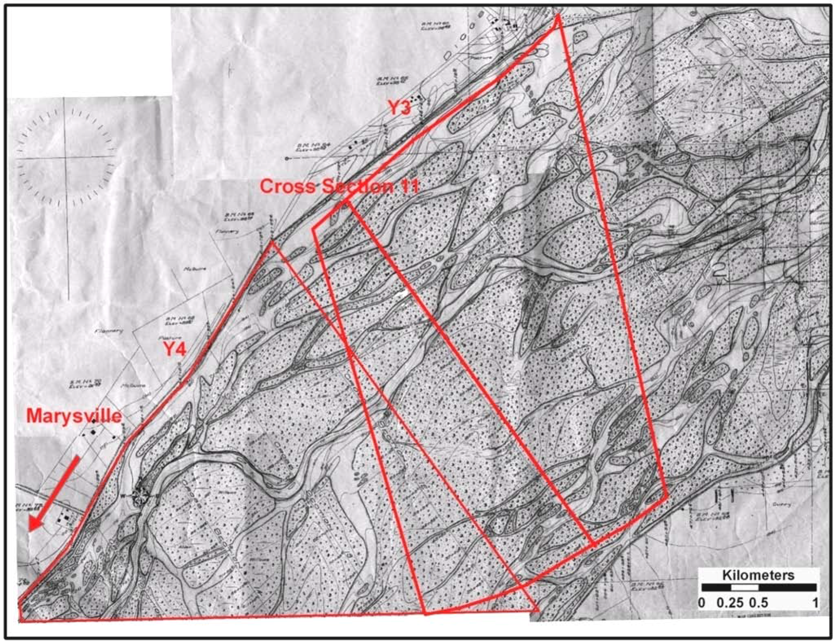
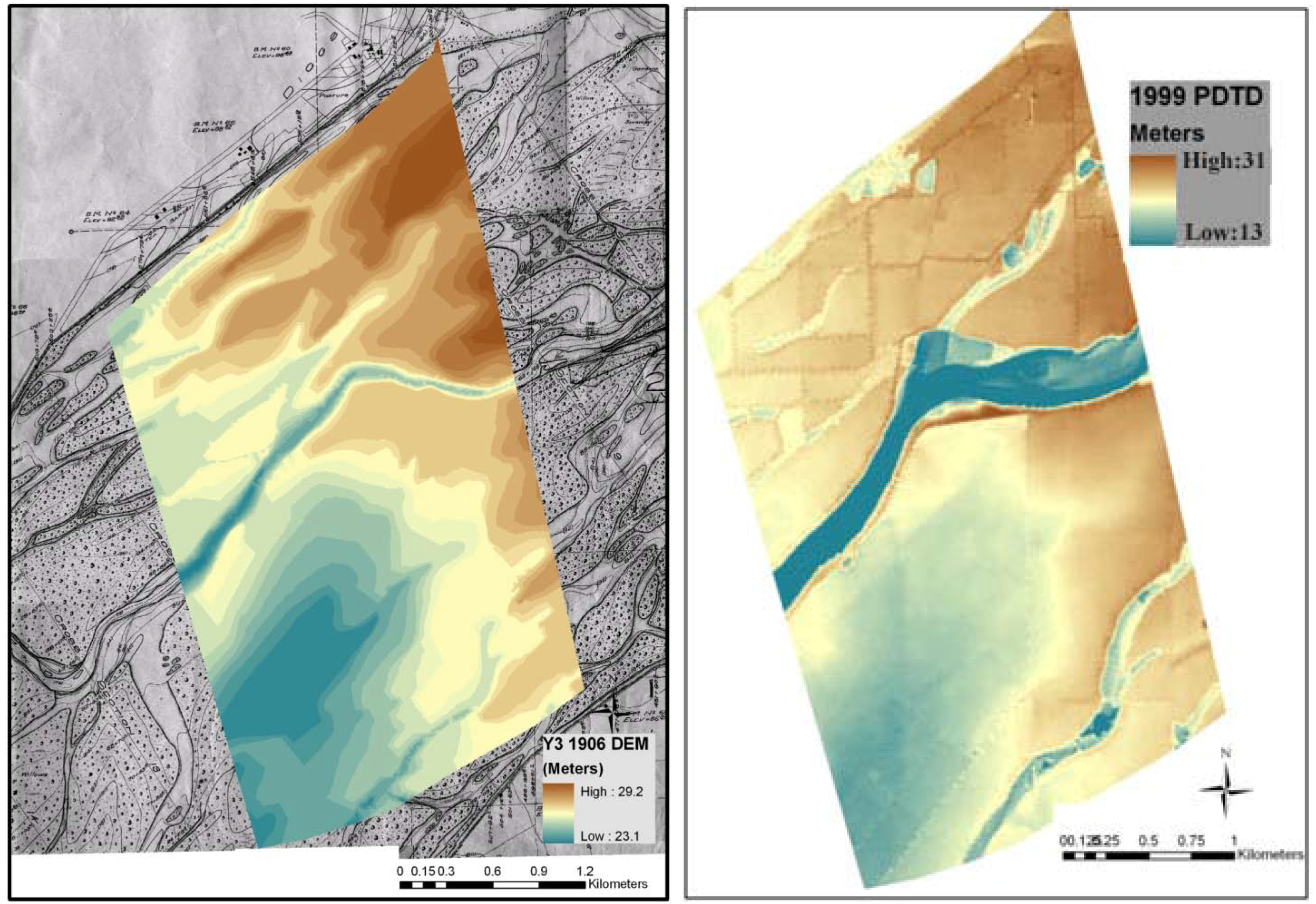
The CDC (1906) maps show detailed topography of the channel, floodplain, and terrace surfaces. The main channel position at these two sites, digitized from a 1999 DOQQ, corresponds fairly closely with the 1906 low-water channel position indicating that the channel largely returned to its original position in this part of the lower Yuba [18]. Channel scars on the 1906 maps represent pre-1906 channel positions during the period of mining. The largest of these high-water channels remain active during large floods. The volumetric analysis reveals that erosion dominated at both Yuba River sites from 1906 to 1999. Total volumetric erosion at the Y3 site was 5.6 × 10⁶ m³ while the total volumetric deposition was 3.9 × 10⁶ m³ (Table 1). The maximum amount of erosion was from the channel bed followed by bars and terraces. On the basis of the two dates of the volumetric analysis, it is not possible to further constrain when these changes occurred.

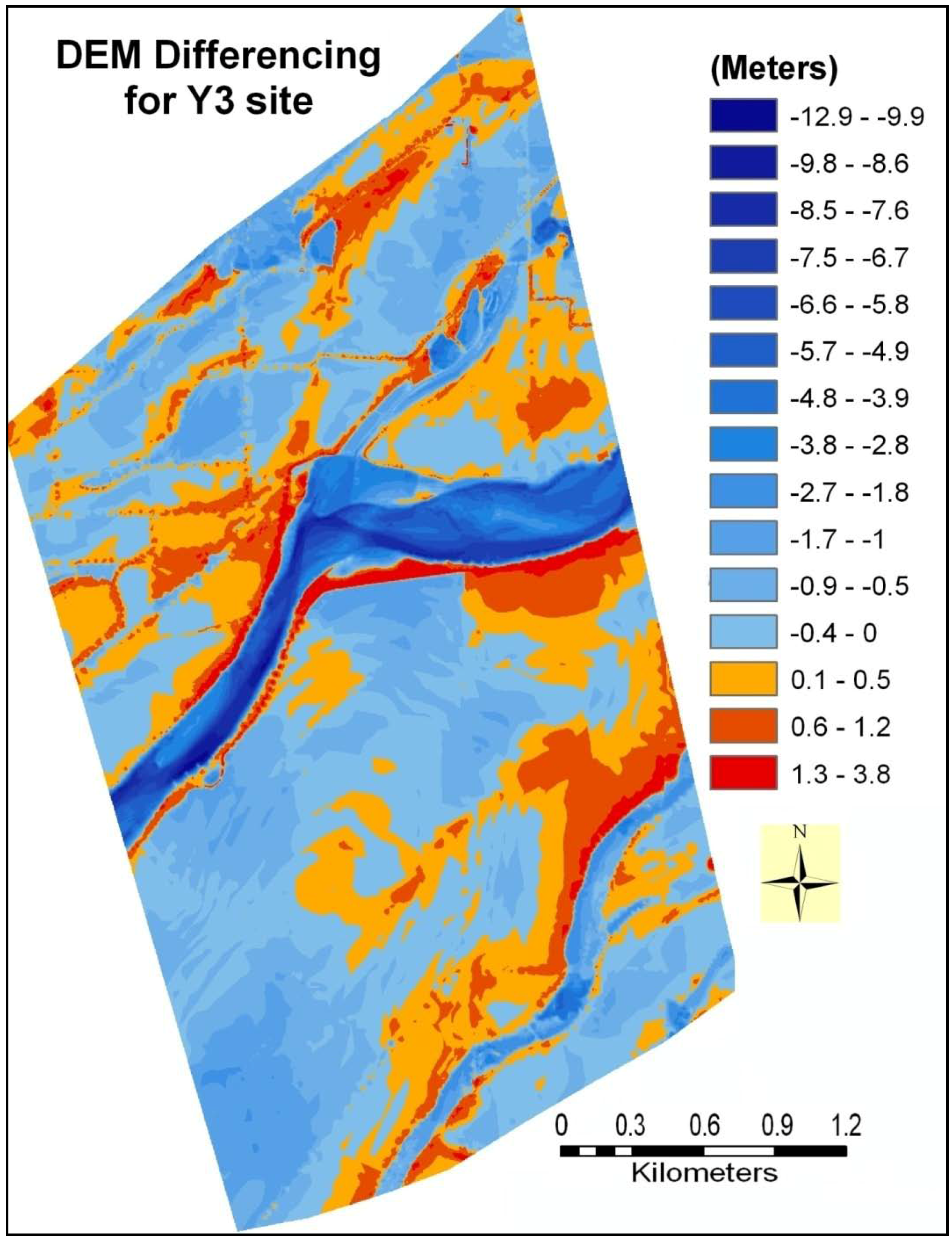
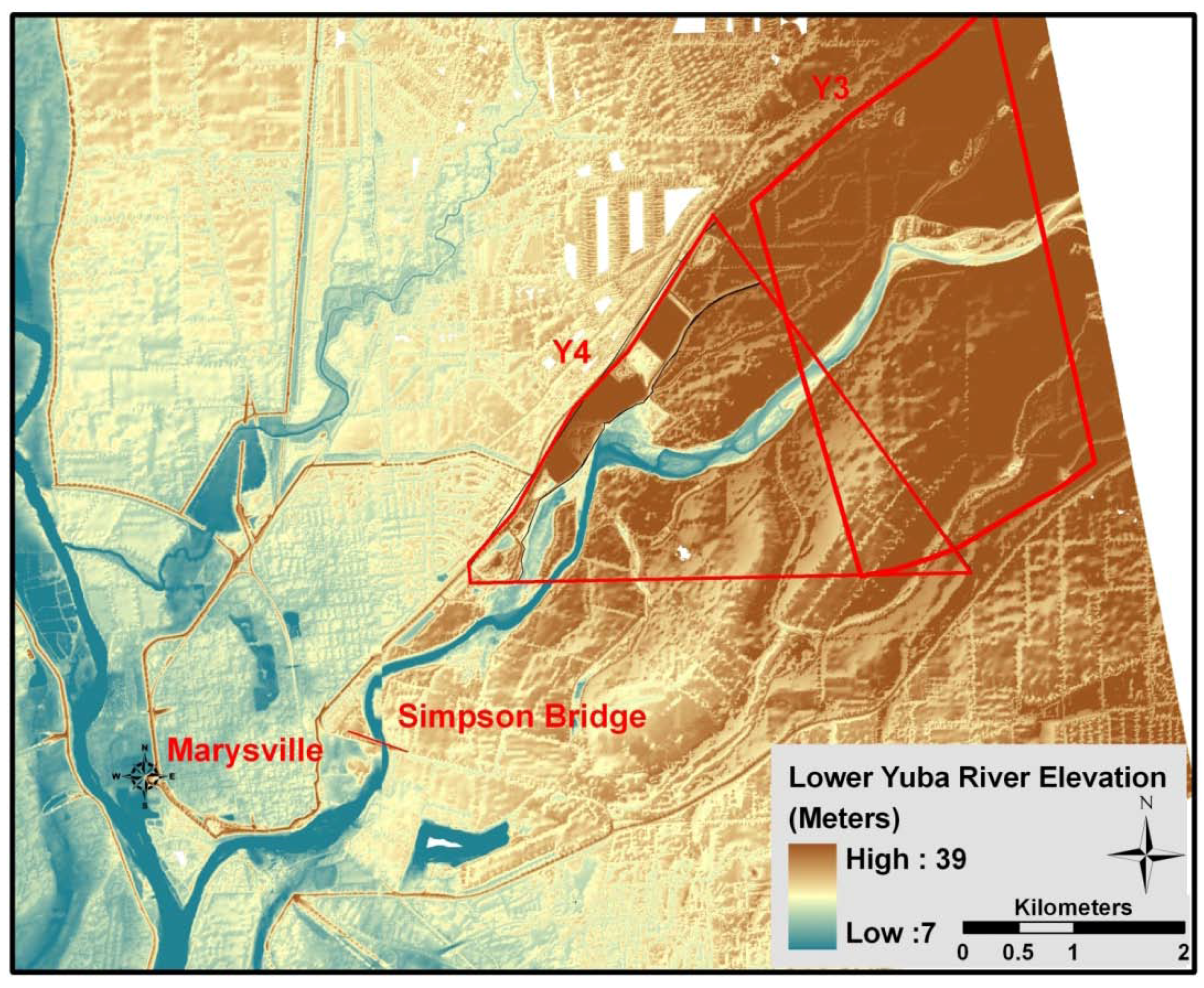
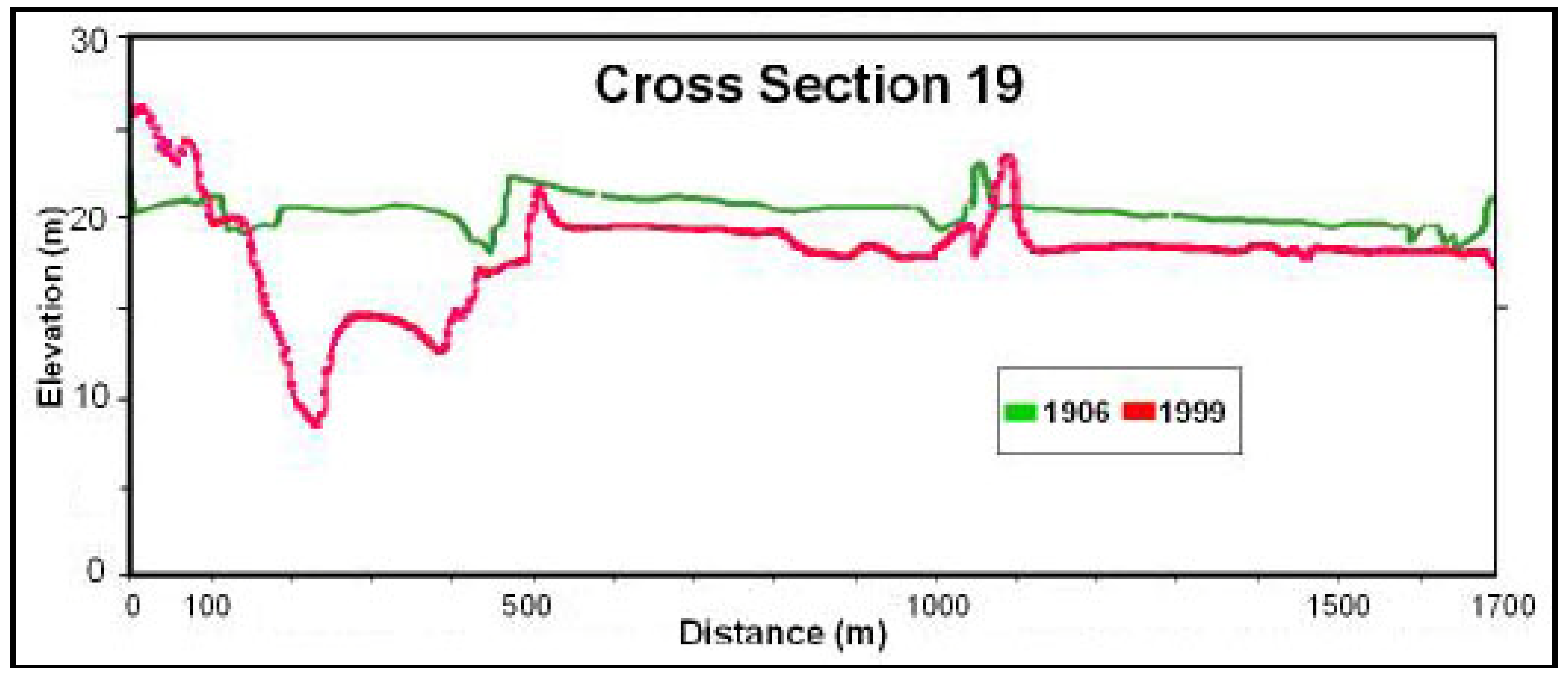
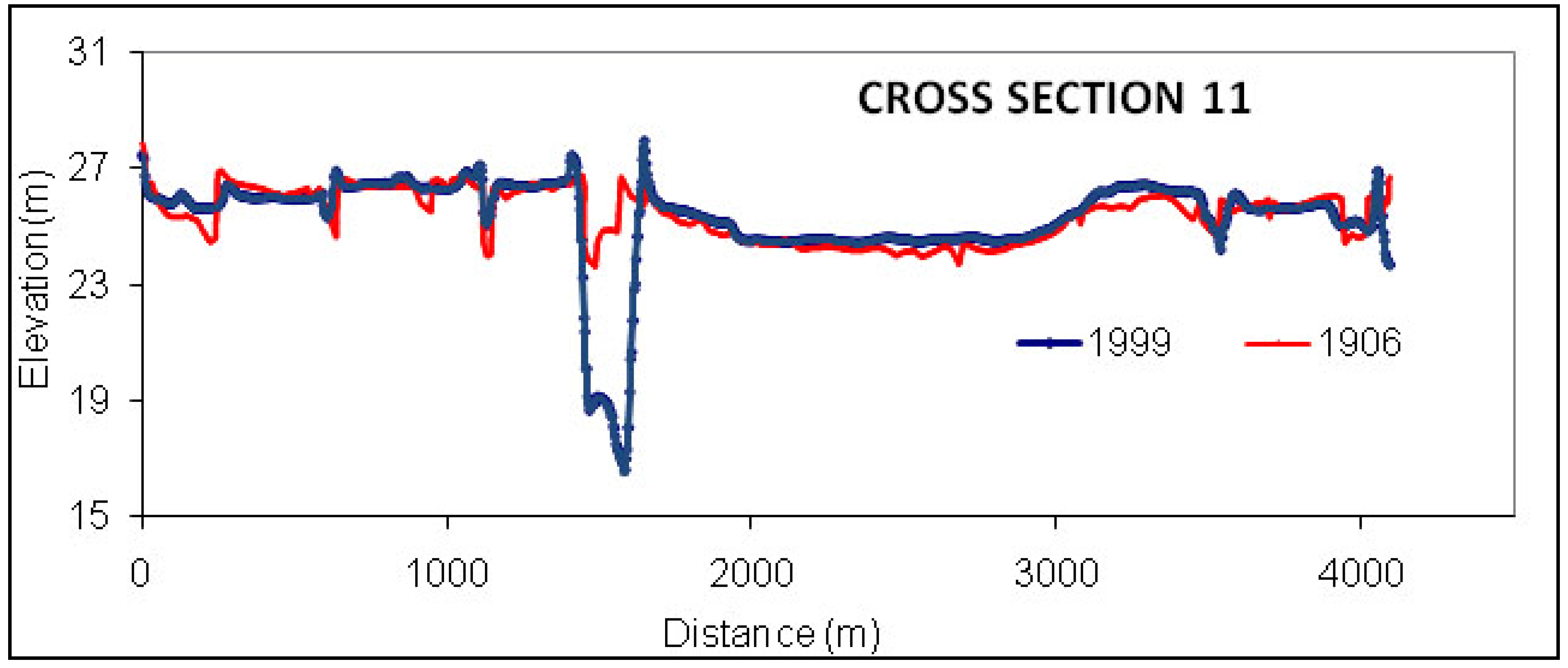
In a broad sense, the volumetric change data are best described in two distinct systems: the main channel versus the terraces (historical floodplains). No deposition occurred in the positions of modern main channels, which were dominated by deep incision, in some areas more than 10 m (Figure 10 and Figure 11). For example, the deepest point in the channel through the Y3 reach is at an elevation of 26.8 m above m.s.l. on the 1906 map, but the deepest point is twelve meters lower at only 14.8 m above m.s.l. when the 1999 SONAR data were collected. Similarly, cross-section analysis (Figure 8) shows that the 1999 channel incised more than 12 m along cross section 11 after 1906. The greatest elevation decreases occurred where the modern thalweg has eroded into relatively high terraces composed of historical mining sediment deposited during the peak period of channel aggradation. At these locations, terrace scarps may exceed 10 m in height and lateral connectivity between the low-flow channel and adjacent alluvial land has been largely disrupted.

Outside of the main channels, changes from 1906 to 1999 were dominated by morphologic adjustments within and along the major high-water channels representing former large channels south of the modern main channel. The high-water channels generally incised one or two meters from 1906 to 1999; far less than the modern main channels. Some isolated points along the high-water channel in the Y3 reach were up to 5 m lower in 1999 than in 1906 (Figure 10), but field visits indicate that these depressions represent local sand quarries. Most sediment deposition in the study area was on terraces; i.e., historical floodplains now perched 6 to 10 m above the main channel but flooded by decadal flood events. Terrace deposits primarily formed as large natural levees adjacent to the high-water channels sometime after 1906, representing a large volume of sediment storage. Overbank sedimentation on natural levees was important during the recovery period along the larger high-water channels as well as the main channel. A logical inference from the dominance of natural levees as depositional sites is that overbank sediment was relatively coarse grained (sandy) and remained close to channel sources. Similar processes have been noted on the Sacramento River at Fremont Weir [29]. Construction of natural levees represents a major redistribution of historical sediment storage from the inner channel, which incised deeply, to floodplains adjacent to major flood channels. Away from channels, broad areas of floodplain surface show a relatively uniform vertical lowering, largely less than 1 m (Figure 10 and Figure 11). Floodplains do not generally erode to such uniform depths, so this may represent compaction of the deep historical deposits, subsidence owing to groundwater extractions, or an artifact of vertical registration.

No deposition occurred in the main high-water channels over the 1906 to 1999 period. Absence of deposition in these channels from 1906 to 1999 raises the question why they are not filling by overbank accretion processes which is typical of abandoned channels on actively inundated floodplains with abundant sediment. The explanation may be that the poor time resolution (1906 to 1999) of the volumetric analysis fails to capture recent filling episodes. Channel incision was likely most active during the early 20th century, and by differencing DEMs over such a long time period, the analysis cannot detect a late period of channel filling of a lower magnitude than the earlier incision. The volumetric results only show the net sediment change on the floodplain for a 93 year period. The total net change in sediment volume from the Y3 site is 1.7 × 10⁶ m³ for the period between 1906 and 1999, but this masks the active relocation of larger sediment volumes including 5.6 × 10⁶ m³ eroded and 3.9 × 10⁶ m³ deposited (Table 1).

Table 1. Volumetric changes from 1906 to 1999 at Y3.

	Erosion (m3)	Deposition (m3)	Net Change (m3)
Channels	−1,935,044	0	−1,935,044
Bars	−1,694,310	937,038	−757,272
High-water channels	−564,605	0	−564,605
Terraces	−1,452,474	2,994,265	1,541,791
Total	−5,646,433	3,931,303	−1,715,130

Table 1. Volumetric changes from 1906 to 1999 at Y3.

	Erosion (m3)	Deposition (m3)	Net Change (m3)
Channels	−1,935,044	0	−1,935,044
Bars	−1,694,310	937,038	−757,272
High-water channels	−564,605	0	−564,605
Terraces	−1,452,474	2,994,265	1,541,791
Total	−5,646,433	3,931,303	−1,715,130

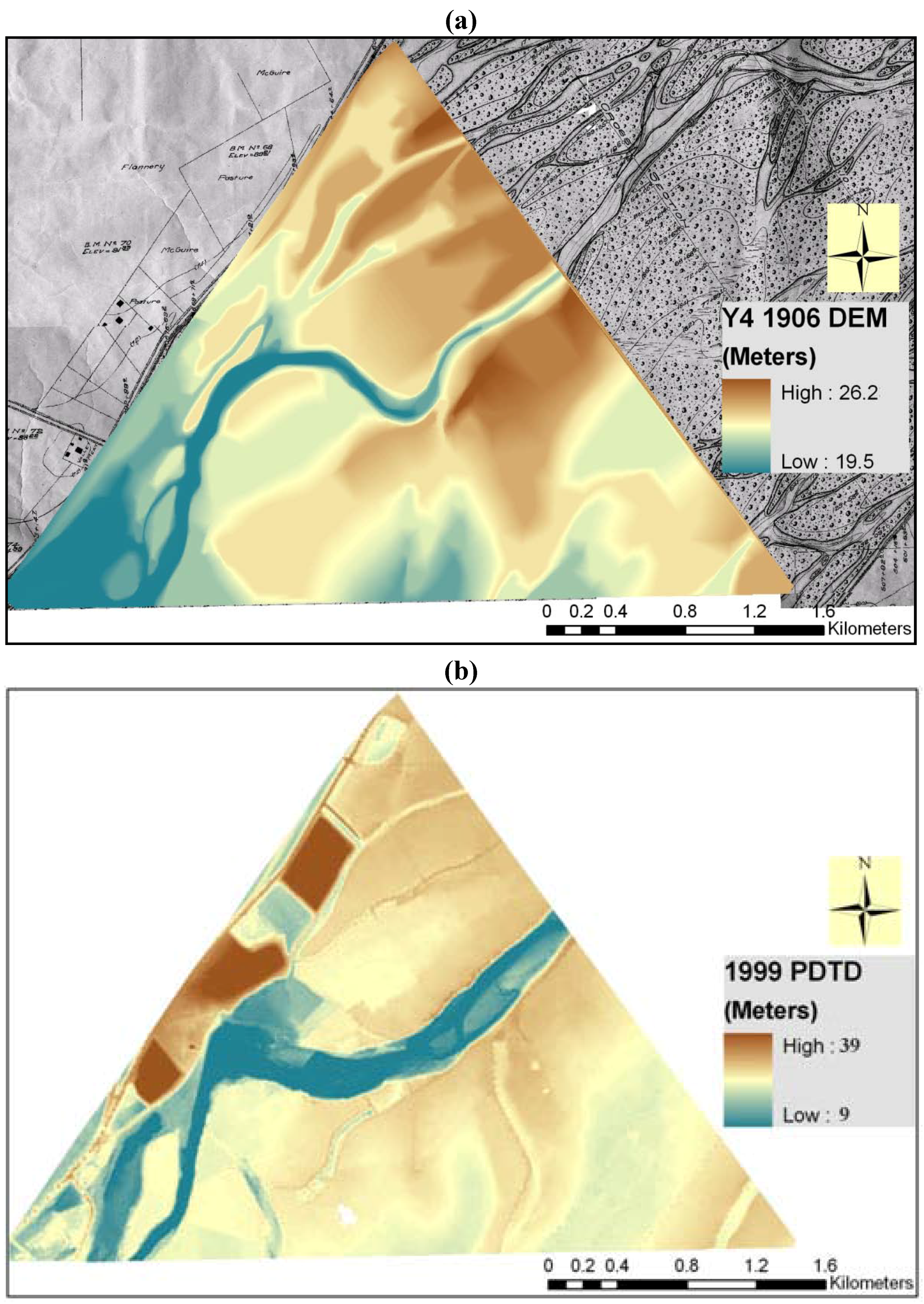
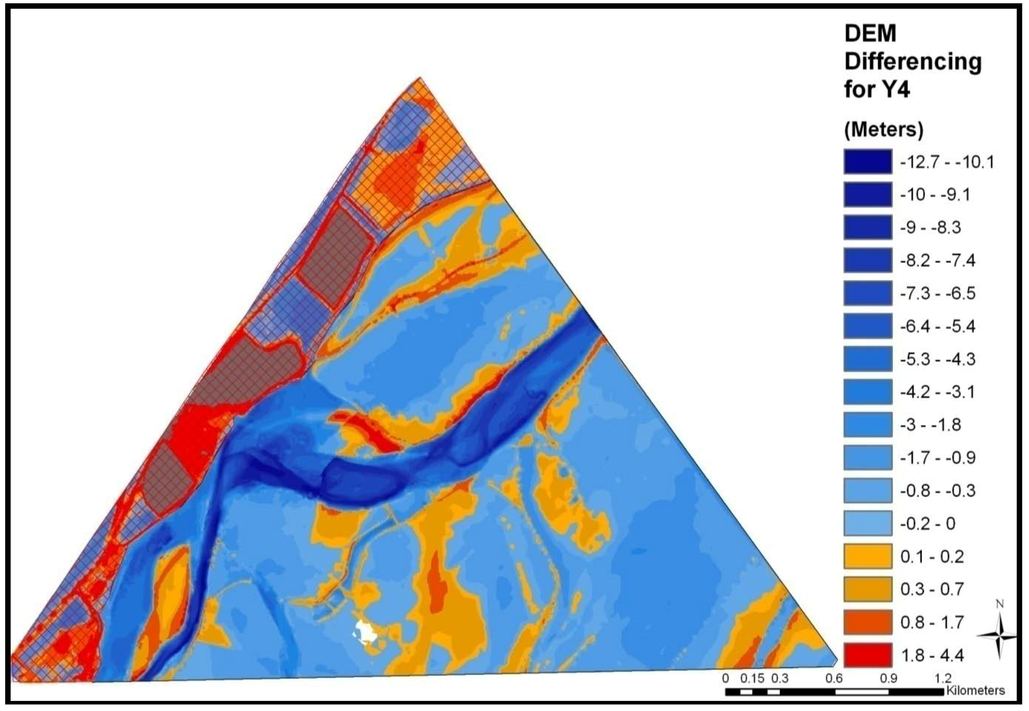
The CDC (1906) map at Y4 site shows similar landform features as the Y3 site. The floodplain is 3.9 km wide. In 1906 the deepest point in the channel at the Y4 site was at an elevation of 24.8 m above m.s.l., while in 1999 the deepest point was 12.1 m lower at 12.7 m above m.s.l. A portion of the north-western bank of the river was masked out and omitted from the Y4 site volumetric analysis owing to the presence of a landfill (Figure 11). Similar to erosion at Y3, the maximum amount of erosion at site Y4 occurred in the channels followed by emergent bars, high-water channels and terraces (Table 2). The areas of the 1999 channel all experienced substantial incision since 1906. A reach of channel along the north bank of the modern channel, in the center of the image, filled during this period. This deposition, classified here as ‘bar’ sedimentation, represents a relatively recent avulsion that is documented in the planimetric analysis. Channel bars received the maximum volume of deposition followed by terraces and high-water channels. Unlike at reach Y3, high-water channels received a considerable amount of deposition. In addition, a thin layer of sediment (0–0.6 m deep) was deposited widely across the floodplain (Figure 11), presumably owing to vertical accretion by overbank flow. While natural levees clearly formed along the modern main channel and high-water channels, they are less massive or extensive than in the Y3 reach. This could represent a distal decline in overbank sediment supplies downstream from the Yuba Gold Fields, although more analysis is needed to test this possibility. The net change in sediment volumes at this site for the 93-year period was an erosion of 5.1 × 10⁶ m³ with a total erosion of 7.1 × 10⁶ m³ and total deposition of 1.9 × 10⁶ m³.

Table 2. Volumetric changes from 1906 to 1999 at Y4.

	Erosion (m3)	Deposition (m3)	Net Change (m3)
Channels	−4,620,498	0	−4,620,498
Bars	−1,344,385	998,223	−346,162
High-water channels	−693,641	310,676	−382,965
Terraces	−409,834	674,689	264,854
Total	−7,068,359	1,983,587	−5,084,771

Table 2. Volumetric changes from 1906 to 1999 at Y4.

	Erosion (m3)	Deposition (m3)	Net Change (m3)
Channels	−4,620,498	0	−4,620,498
Bars	−1,344,385	998,223	−346,162
High-water channels	−693,641	310,676	−382,965
Terraces	−409,834	674,689	264,854
Total	−7,068,359	1,983,587	−5,084,771

4.2. Planimetric Analysis

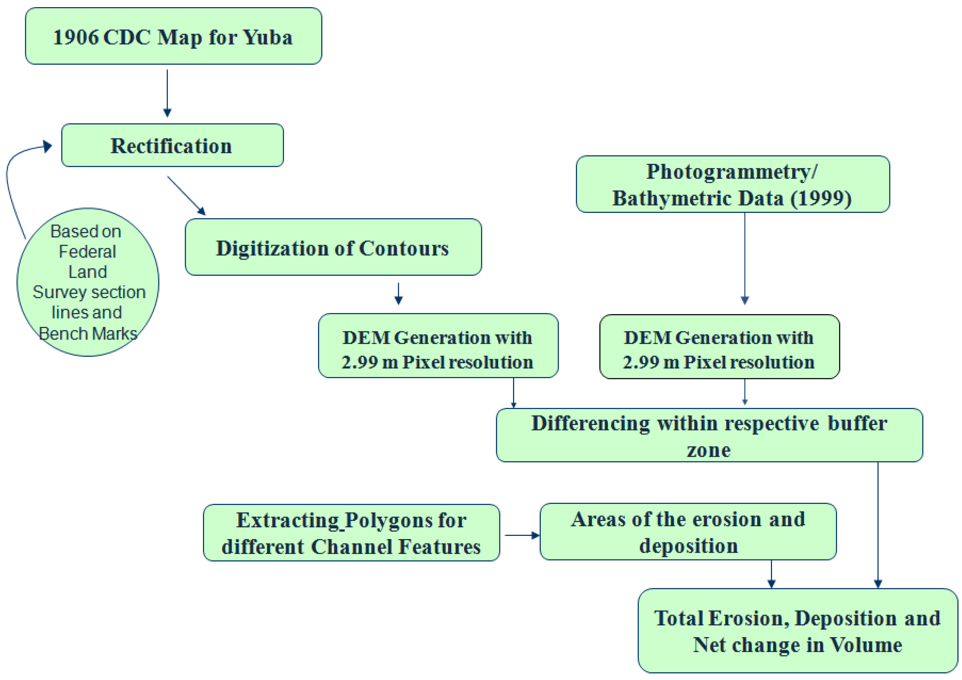
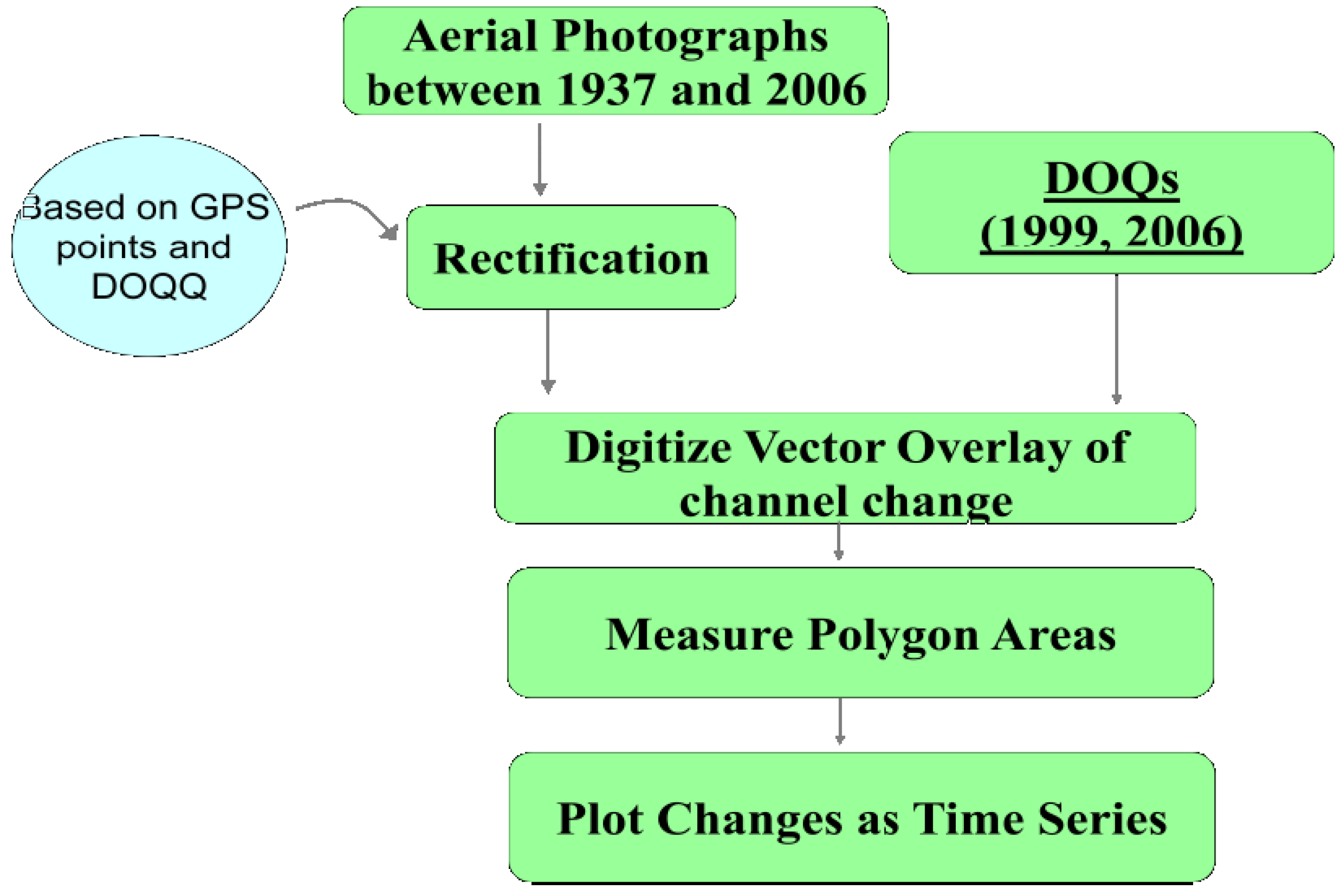
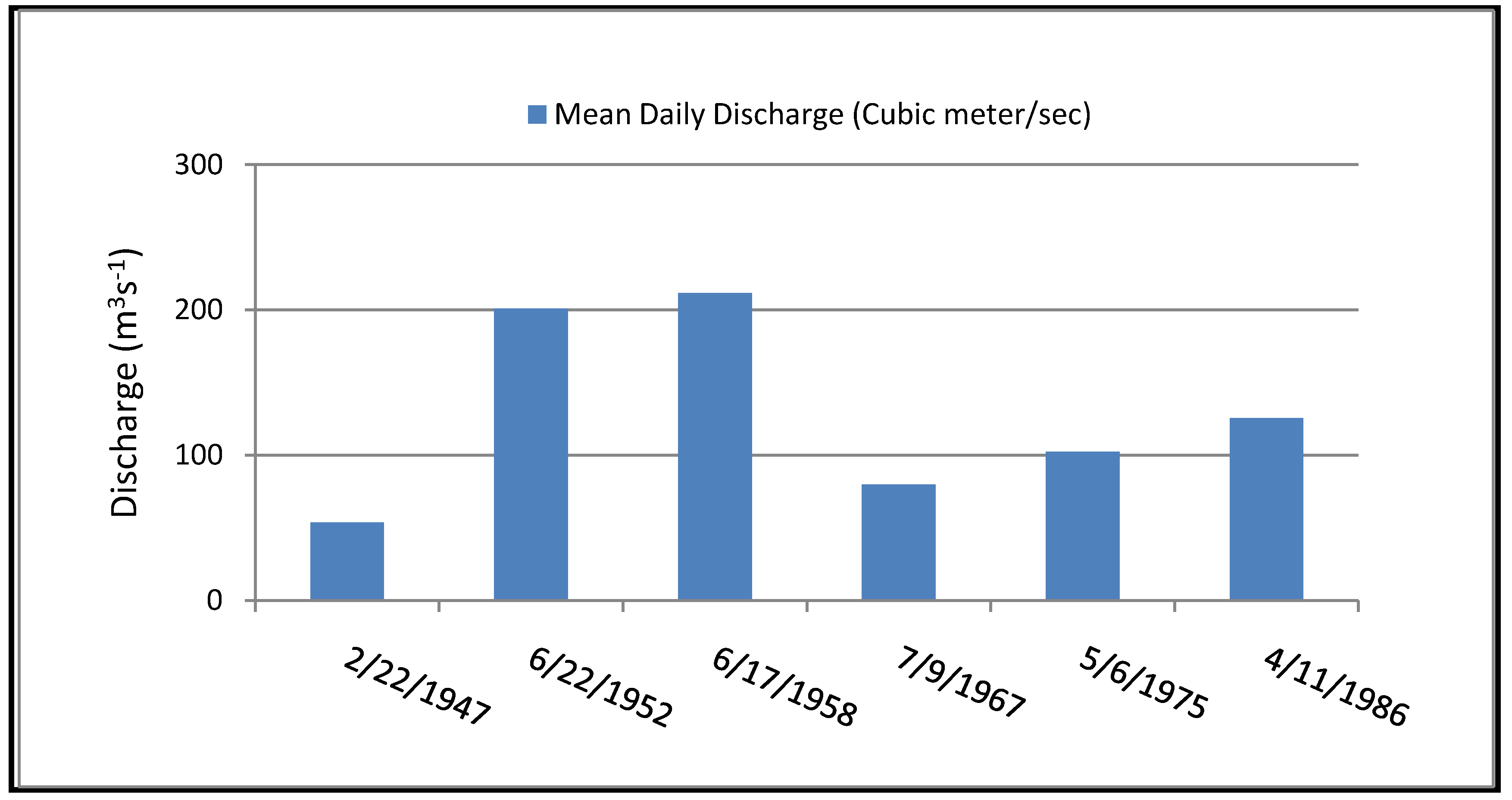
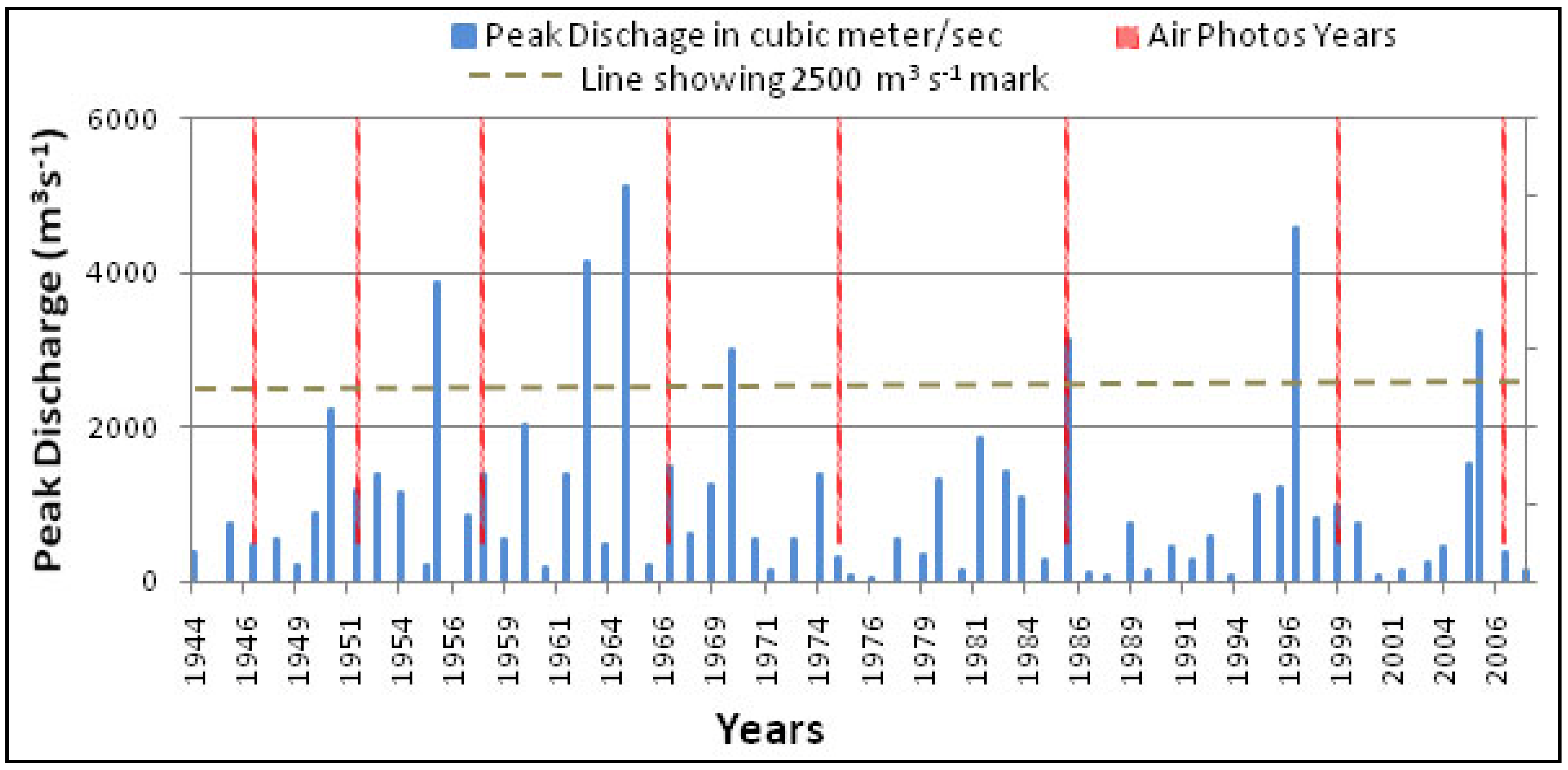
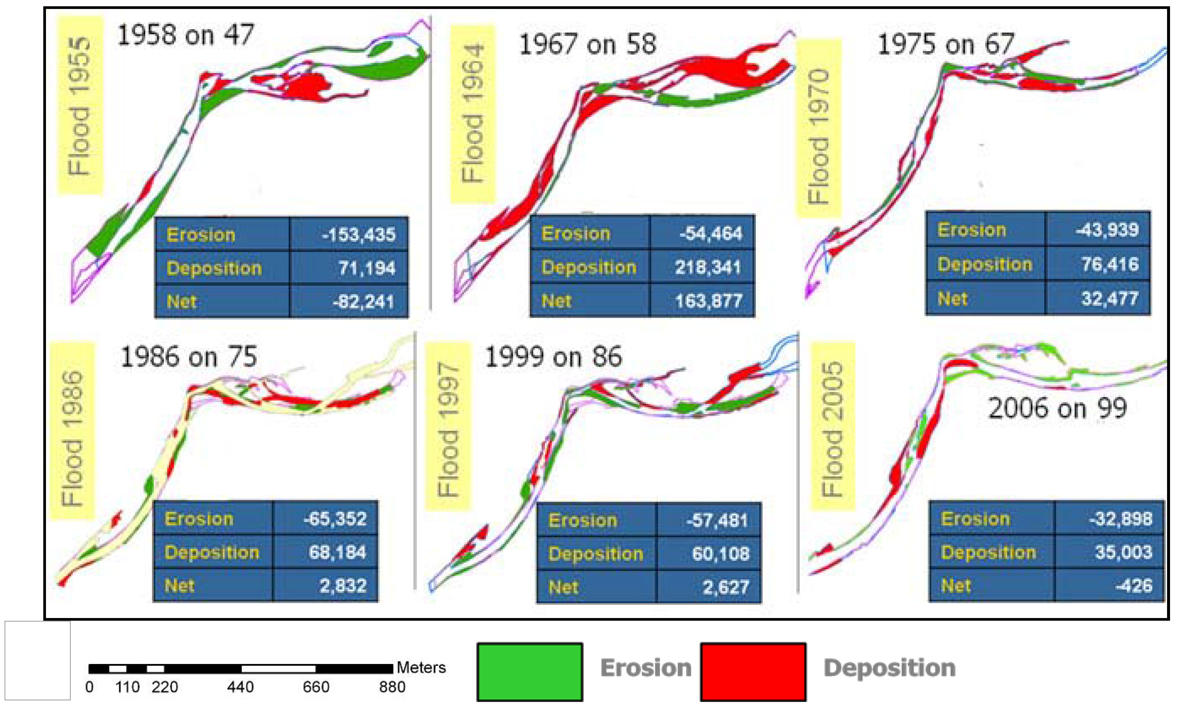
Spatial and temporal variations in channel enlargement, lateral migration, and associated surface areas of within-channel erosion and sedimentation were measured based on a remote sensing and GIS analysis of 1906 California Debris Commission (CDC) topographic maps [26], aerial photographs flown between 1947 and 2006 (NAPP), DOQQs from 1999, 2006, and 1999 photogrammetric data (USACE [24,25]). These data were used to reconstruct historical channel changes and to calculate surface areas of erosion and sedimentation. Aerial photographs bracketing major flood years for Y3 (Figure 14) were used to measure changes in surface area corresponding to erosion and deposition by a given flood. For example, the overlay analysis between 1952 and 1958 aerial photographs reveals changes corresponding to erosion and deposition by the 1955 flood. The following sets of maps show total erosion and deposition at Y3 and Y4 for each period followed by bar charts of erosion and deposition for each period broken into bars and terraces. In this post-incision period, the replacement of water by new areas of land is always classified as ‘bars’ because deposition on high terraces cannot be detected by planimetric analysis which measures lateral migration.

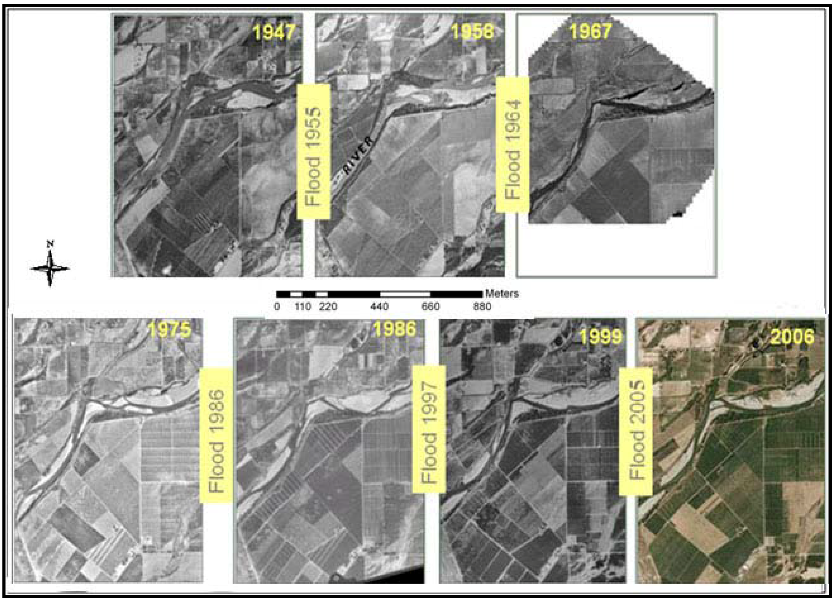
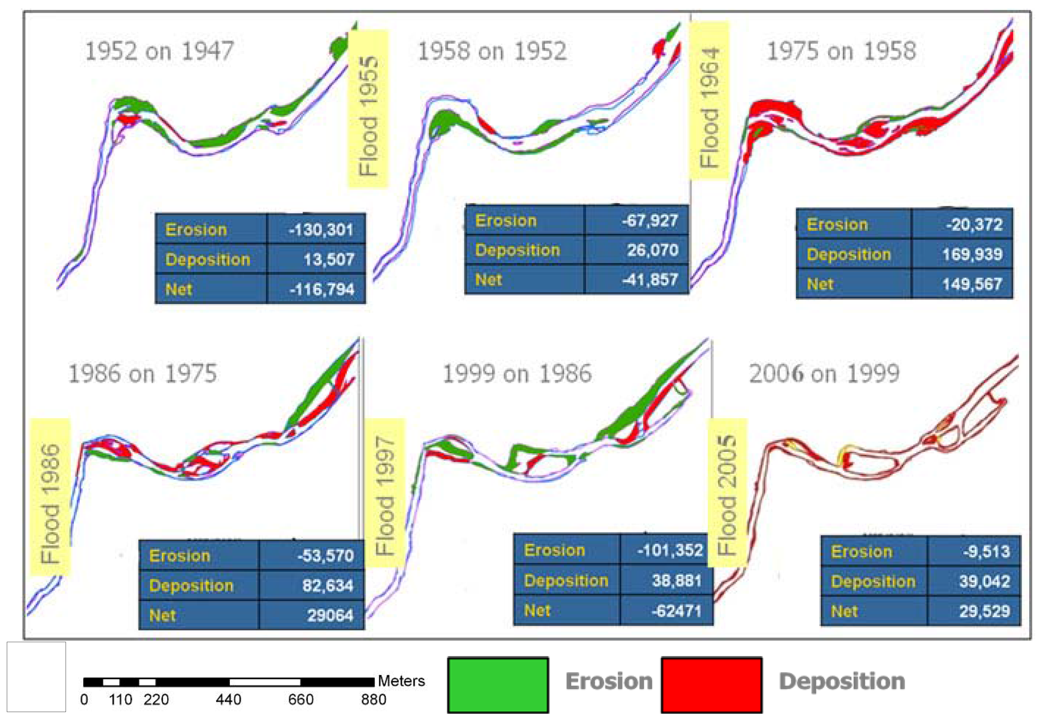
Changes in surface area at Y3 due to erosion and deposition by six different floods are shown in Figure 17 and Figure 18. The maps illustrate a greater amount of surface change in the first half of the century until 1960 with decreased lateral activity thereafter. In addition, the active zone of lateral channel activity apparently narrowed in the later period. The 1955 flood resulted in substantial net erosion of bars and terraces, whereas the 1964 flood deposited a considerable amount of sediment in channels to form new bars (Figure 18). The net change for each period drops to a negligible value after 1986, but this does not indicate a lack of channel activity. Instead, it represents bar deposition in each period that is approximately equal to erosion.

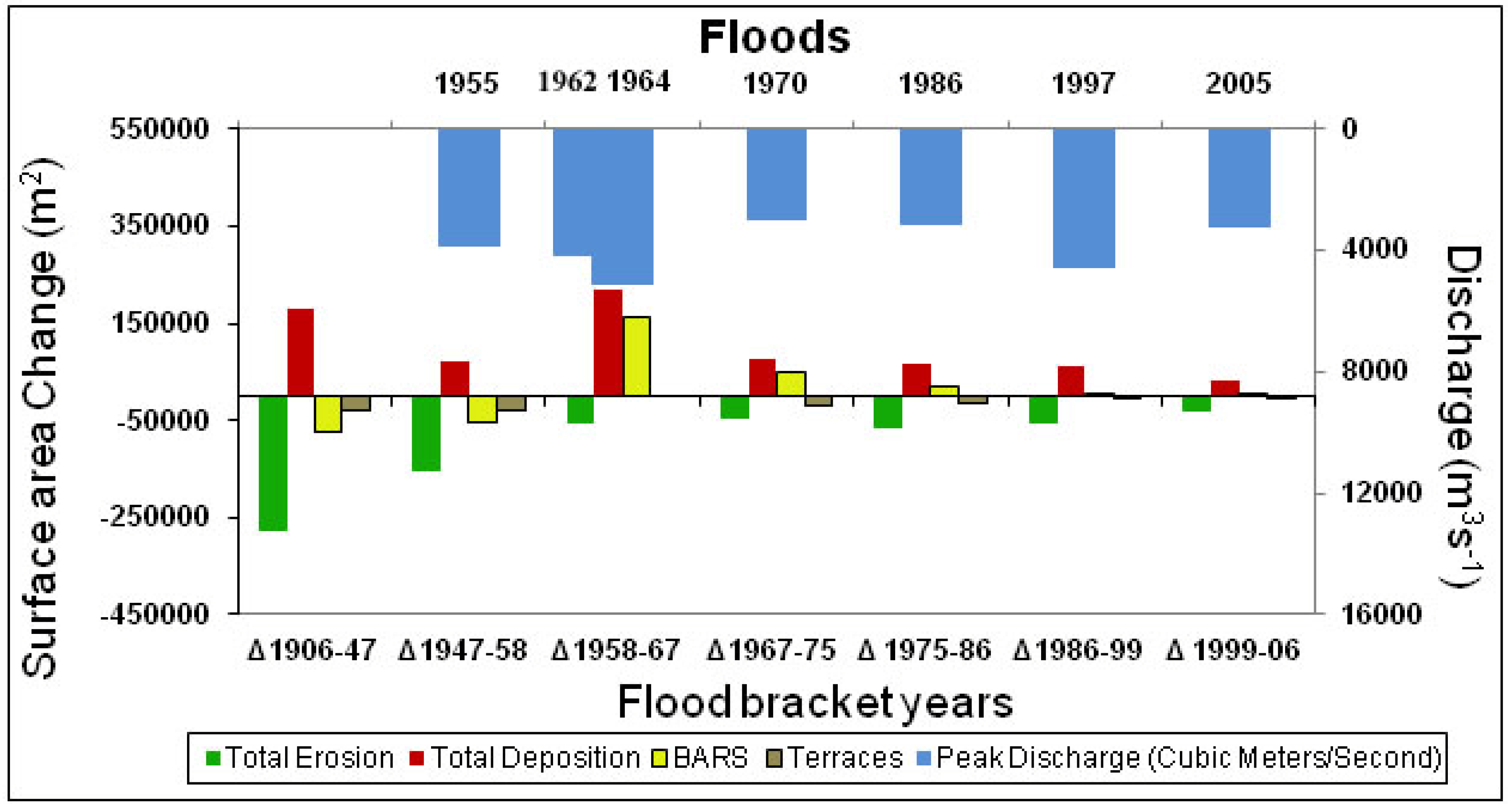
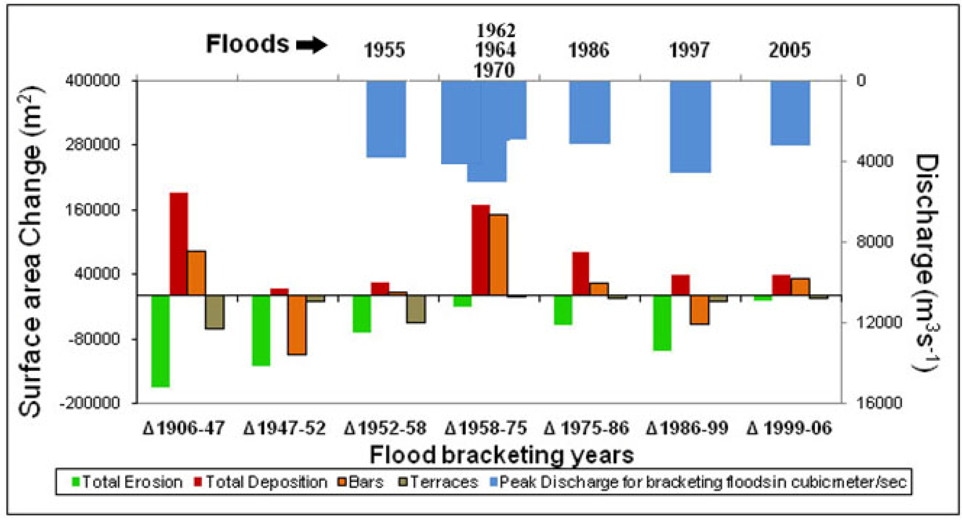
Areal changes separated into bars versus terraces and into total erosion and total deposition (Figure 19) reveal several features of channel change. Changes in bar and terrace surface areas on these bar charts represent net change (deposition − |erosion|), however, so values can be much smaller than total bar erosion or total terrace erosion. Both erosion and deposition were highly active in the early period as shown on the bar graph (Figure 19). Creation of ~150 × 10³ m² of new surface by the 1964 flood was entirely on lower surfaces classified here as emergent bars. Some of this deposition may be an artifact of the low discharge at the time that the 1967 aerial photograph was flown (Figure 9), although that stage change was less than one meter. A moderately large flood in 1970 was presumably responsible for the deposition on bars that occurred between 1967 and 1975 over a surface extent of ~50 × 10³ m². The 1986 and 1997 floods had high peak discharges, but a smaller surface area of bars or terraces was displaced by these floods.

In general, the areas of net erosion, net deposition, and total net change appear to have decreased somewhat after the 1964 flood and certainly after the 1986 flood (Figure 17, Figure 18, Figure 19). Erosion and deposition continued throughout the study period. In fact, a major channel avulsion occurred on the south bank of the upper reach in response to the 1997 flood. A reduction in lateral activity did occur later in the study period, however, such that lateral migration and point bar formation became confined to a narrower band. This was independent of flood magnitudes which did not decrease during the period of study (Figure 19).

Figure 17. Erosion and deposition polygons showing areas of sediment reworked at the Y3 site for the period between 1906 and 1947. Table shows changes in area due to erosion, deposition and net change. Areas are in square meters.

Figure 17. Erosion and deposition polygons showing areas of sediment reworked at the Y3 site for the period between 1906 and 1947. Table shows changes in area due to erosion, deposition and net change. Areas are in square meters.

Figure 18. Erosion and deposition polygons showing areas (m²) of sediment reworked by each flood at the Y3 site. Tables show changes in area due to erosion, deposition and net change for each flood year.

Figure 18. Erosion and deposition polygons showing areas (m²) of sediment reworked by each flood at the Y3 site. Tables show changes in area due to erosion, deposition and net change for each flood year.

Figure 19. Surface areas of total, bar and terrace, erosion and deposition corresponding to each flood period at the Y3 site. Positive area changes represent deposition; negative area changes are erosion. Values of total erosion and total deposition are for bars plus terraces, while values of bars and terraces represent net changes from erosion plus deposition.

Figure 19. Surface areas of total, bar and terrace, erosion and deposition corresponding to each flood period at the Y3 site. Positive area changes represent deposition; negative area changes are erosion. Values of total erosion and total deposition are for bars plus terraces, while values of bars and terraces represent net changes from erosion plus deposition.

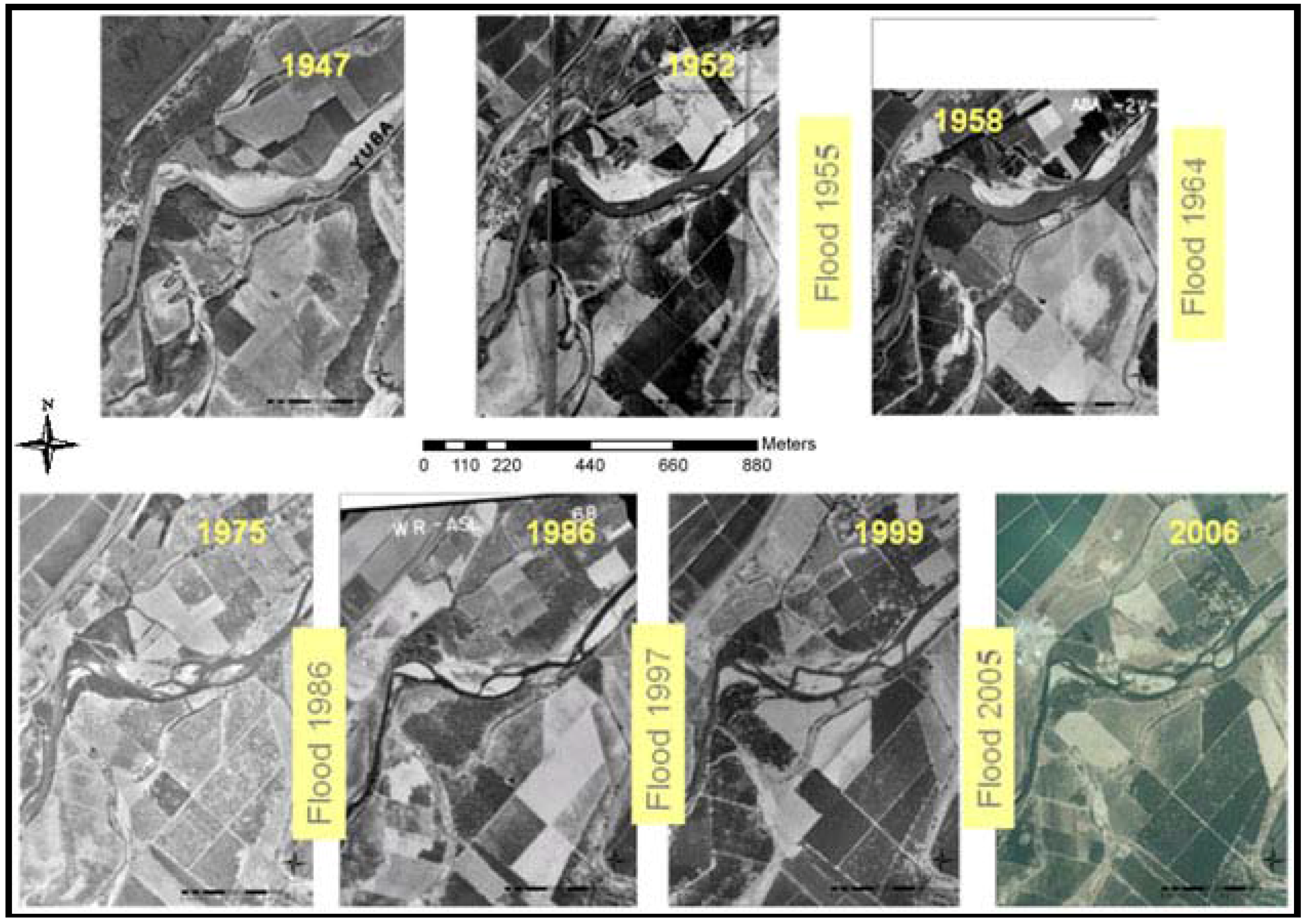
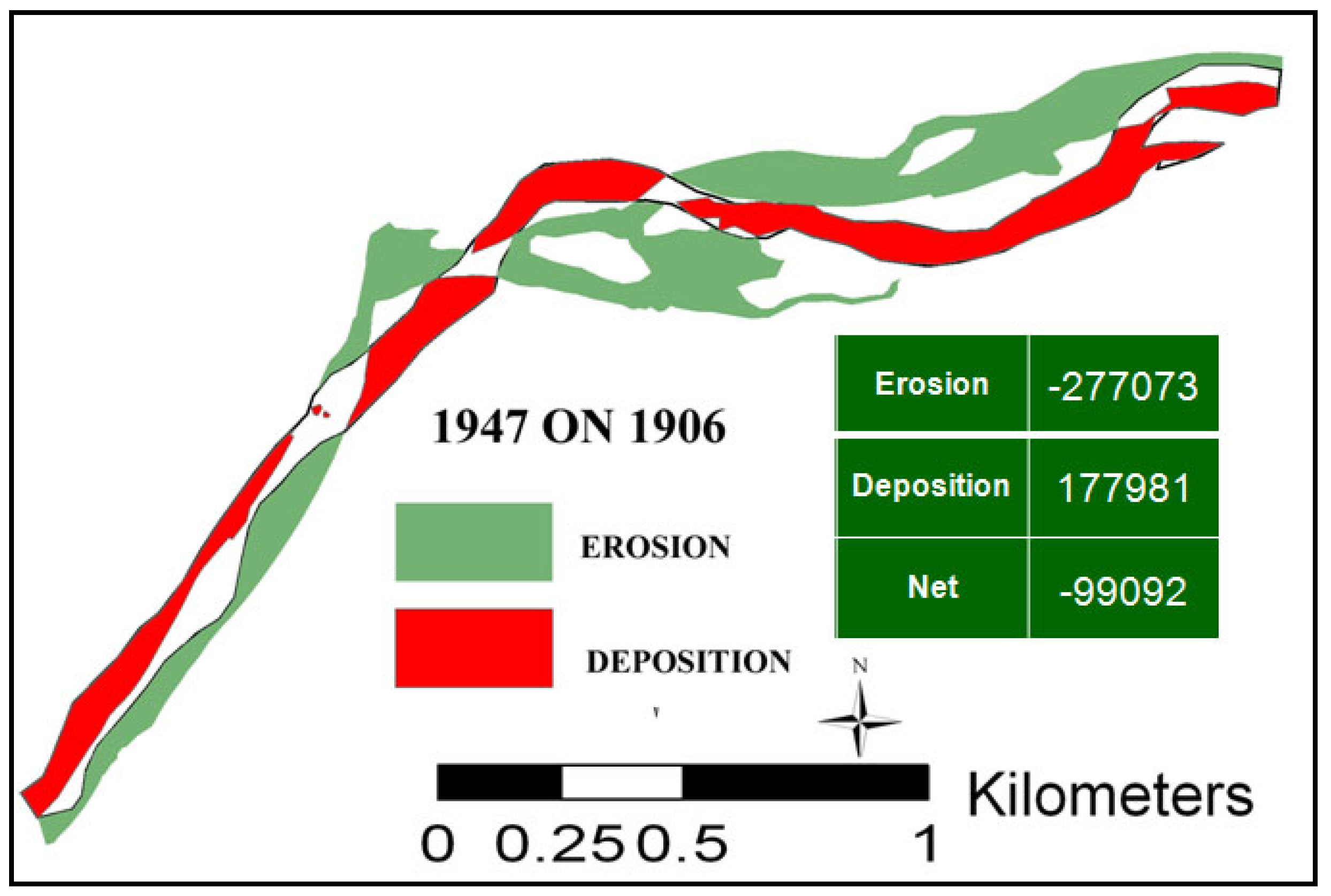
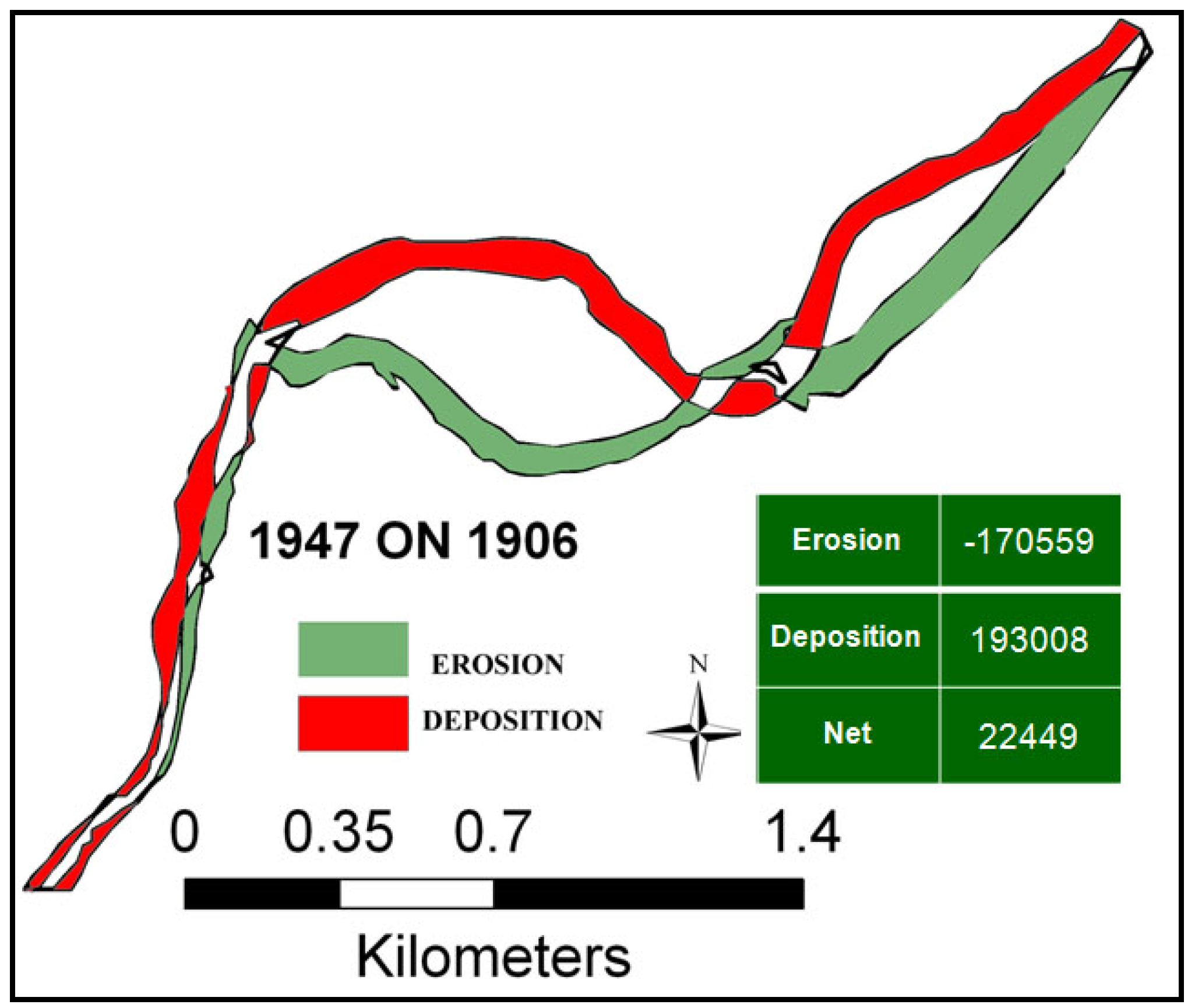
Similar planimetric results are obtained for the Y4 site, where major avulsions and expanses of lateral migration occurred in the early period 1906 to 1947 (Figure 20). These avulsions were associated with large areas of erosion and deposition, 17 × 10³ m² and 193 × 10³ m², respectively, but only modest areas of net change. These areas of erosion and sedimentation are the largest for any single period, although comparability is limited by the longer duration of time.

Figure 20. Erosion and deposition polygons showing areas (m²) of sediment reworked at Y4 site for the period between 1906 and 1947. The table shows the change in area due to erosion, deposition and net change.

Figure 20. Erosion and deposition polygons showing areas (m²) of sediment reworked at Y4 site for the period between 1906 and 1947. The table shows the change in area due to erosion, deposition and net change.

Subsequently, the 1955 flood eroded ~42 × 10³ m² of terrace surfaces and the 1964 flood deposited sediment creating ~150 × 10³ m² of new bar surfaces (Figure 21 and Figure 22). As at the Y3 site, the 1986 and the 1997 floods displaced smaller areas compared to the earlier floods at the Y4 site, although the magnitude of the later floods are no less than the earlier floods. The 1997 flood (Q = 2,793 m³s⁻¹; 161,000 ft³s⁻¹) had a higher peak discharge than the 1955 flood (Q = 2,515 m³s⁻¹; 136,000 ft³s⁻¹) (U.S. Geological Survey gauge data).

Two large deposition events are documented by the planimetric data from the 1950s through the 1970s. The Y3 site experienced ~200,000 m² of bar deposition in 1964 and the Y4 site experienced almost as much deposition in the 1970s. The Y3 deposition event is explained by a substantial channel avulsion in the northern section of the reach that caused abandonment of a large area of the north channel. This increased area of emergent bars was not compensated for by lateral migration of the channel into the south bank indicating that the channel narrowed in the upper reaches of Y3. Deposition at the Y4 site between 1958 and 1975 may best be explained by three factors. First, this was a longer period than most, extending 17 years. Second, two moderately large floods occurred during this period, which apparently caused the channel to narrow and abandon emergent bars. Finally, the 1958 aerial photograph that forms the basis of the depositional area calculation, was a high flow (Figure 9 and Figure 15) that tends to overestimate new exposed bar areas on subsequent images.

A substantial period of erosion occurred from 1975 to 1999 at Y4 in response to lateral migration through the entire period. Migration is shown by the gradual southward movement of the northern eroded channel in the period 1975–1986 that included the 1986 flood and in the period 1986–1999 that included the 1997 flood (Figure 21). Apparently, these changes represent progressive migration across the north bar rather than an avulsion from one location to another. Therefore, it represents the displacement of a large volume of sediment as the thalweg moved across the entire area.

Figure 21. Erosion and deposition polygons showing areas of sediment reworked by floods at the Y4 site. Tables show changes in area (m²) due to erosion, deposition and net change for each flood.

Figure 21. Erosion and deposition polygons showing areas of sediment reworked by floods at the Y4 site. Tables show changes in area (m²) due to erosion, deposition and net change for each flood.

Figure 22. Surface areas of total, bar and terrace, erosion and deposition corresponding to each flood at the Y4 site. Positive area changes represent deposition; negative changes are erosion. Values of total erosion and total deposition are for bars plus terraces, while values of bars and terraces represent net changes from erosion plus deposition.

Figure 22. Surface areas of total, bar and terrace, erosion and deposition corresponding to each flood at the Y4 site. Positive area changes represent deposition; negative changes are erosion. Values of total erosion and total deposition are for bars plus terraces, while values of bars and terraces represent net changes from erosion plus deposition.

4.2.1. Implications of Planimetric Analysis

The planimetric change analysis between 1906 and 1947 shows the highest change in area for both the sites (Figure 19 and Figure 22). Apparently, bar and terrace erosion as measured by planimetric changes was somewhat more active during the early period, from 1906 through the 1970s than the later period from the 1980s onward. The total change in areas due to each flood tends to decrease towards the end of the century (Figure 23) in spite of large floods occurring in the later period. Thus, on the basis of this planimetric analysis, it is not possible to reject the null hypothesis that morphologic changes were not greater during the early 20th century than subsequent changes later. In fact, the original hypothesis appears to be supported by the planimetric analysis; i.e., floods after the 1970s were less effective than in the earlier period. Overall, total areas of planimetric change were fairly similar between sites Y3 and Y4 with the exception of deposition events in the 1960s at Y3 and in the 1970s at Y4 (Figure 19 and Figure 22). Both of those events represent episodic bar formation events that were part of long-term channel morphologic adjustments to decreased sediment loads and channel incision. It is not clear if the downstream shift in the avulsions from Y3 to Y4 through time represents a large-scale systematic trend. Similar to the temporal patterns demonstrated at Y3, areas of net erosion, net deposition, and total net change decreased somewhat in the later period after the 1970 flood (Figure 22). Three floods occurred in the period 1958 to 1975, which limits the ability to resolve which floods within this period were geomorphically effective. It is possible that the timing of the decline in activity is similar between the two sites (compared with Figure 19). This decline was independent of flood magnitudes.

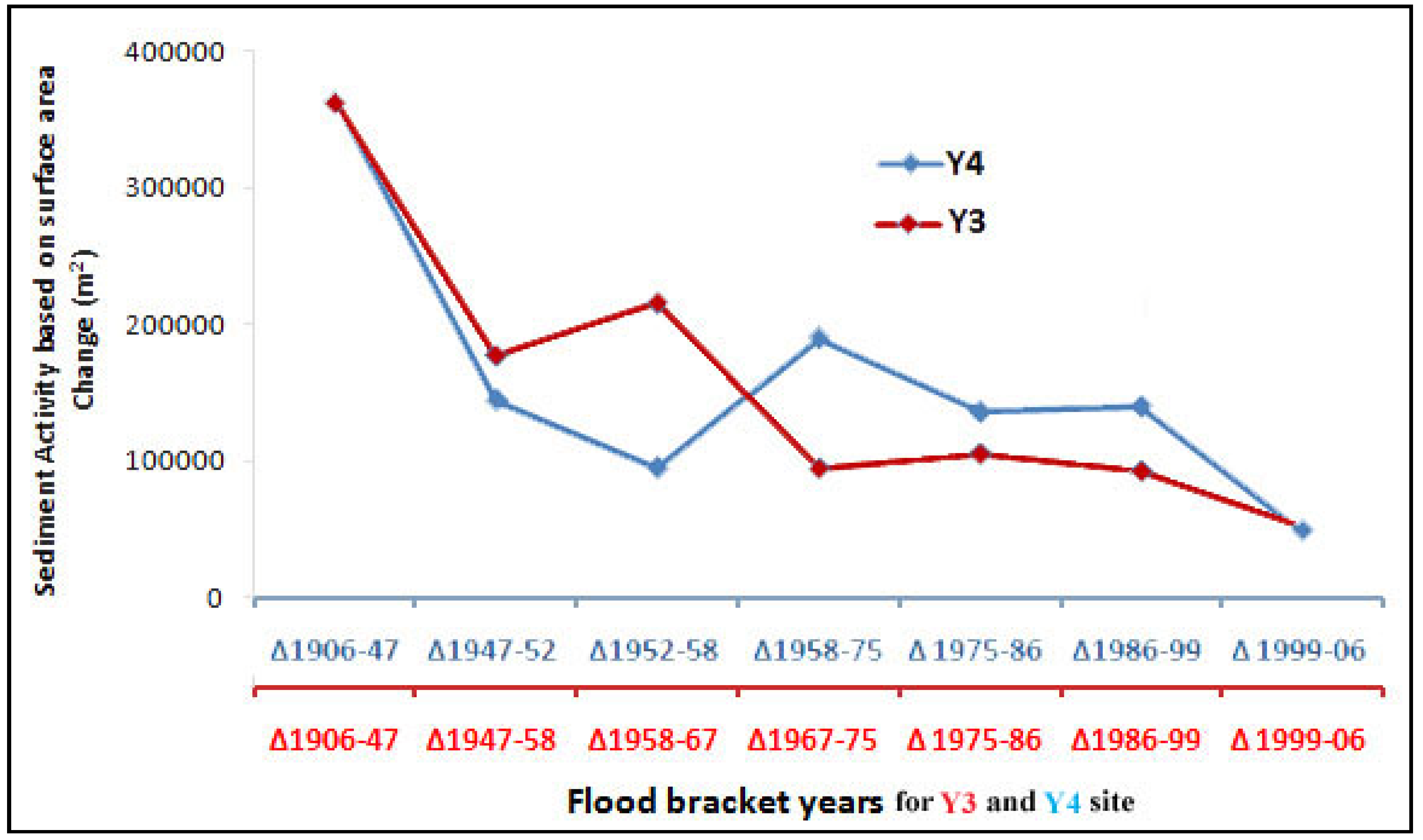
Figure 23. Total amount of sediment displaced (|erosion| + |deposition|) decreased during the later half of the 20th century at both the Y3 and Y4 sites. The X axes are not to scale.

Figure 23. Total amount of sediment displaced (|erosion| + |deposition|) decreased during the later half of the 20th century at both the Y3 and Y4 sites. The X axes are not to scale.

5. Conclusion

Floodplain sedimentation due to hydraulic mining in the Sierra Nevada of California is an extreme example of anthropogenic impacts on a fluvial system. This study shows how remote sensing methods can be used to quantitatively document channel adjustments to this huge deposit and the timing and extent of sediment reworking by floods. Calculations done in this spatially explicit manner provide a distributed model of channel and floodplain adjustment that is useful for applied and theoretical evaluations of how the system has behaved and may be expected to adjust in the future. These patterns of sediment mobilization may affect the flood conveyance system [19]. Volumetric and planimetric analyses show that sediment was reworked and remobilized throughout the period from 1906 to 2006 at the Y3 and Y4 sites. The volumetric study documents net erosion at both sites amounting to 1.7 million and 5.1 million cubic meters was eroded from Y3 and Y4 sites, respectively, over the 93-year period 1906 to 1999. These net values are conservative and mask much larger volumes of total erosion and deposition at both sites. The planimetric analysis shows that substantial reworking of sediment was active throughout the 100-year period from 1906 to 2006, and that reworking and remobilization of HMS during major flood events continued to contribute substantial amounts of sediment to downstream channel reaches. Erosion of bars and terraces dominated during the period of 1906 to 1958 whereas bar deposition became more common from 1958 to 2006. The areal extent of sediment reworking by floods also decreased towards the later part of the century even though flood magnitudes did not decrease. This may signal a transition away from dominance by channel vertical incision as the system relaxed from a period massive aggradation and returned to pre-mining base levels. The processes have apparently shifted to slow (or infrequent) erosion of high terraces—where not precluded by bank protection—that feeds sediment to the channel. Channel bars have become sites of net deposition.

Information derived from this study should help provide an understanding of the long-term environmental impacts of episodic sedimentation on rivers. Contrary to the Gilbert [16] model, which implies that river systems quickly return to their pre-disturbance state following episodic sedimentation, this study shows that channel adjustments to the effects of hydraulic mining may continue in the Central Valley but at a declining rate. Rates of planimetric change declined over the period. Lateral erosion and deposition have largely stabilized at the Y3 site, although they remain active at the Y4 site. Information derived from this study should be useful to river managers concerned with flood and sedimentation problems in the lower Sacramento River in particular and to a conceptual understanding of adjustments to disruptions caused by episodic sedimentation and anthropogenic disturbances to fluvial systems in general.

References and Notes

1. Nanson, G.C.; Croke, J.C. A genetic classification of floodplains. Geomorphology 1992, 4, 459–486. [Google Scholar] [CrossRef]
2. Wolman, M.G.; Leopold, L.B. River Flood Plains: Some Observations on Their Formation; U.S. Geological Survey Professional Paper 1957, 282c; United States Government Printing Office: Washington, DC, USA, 1957.
3. Marcus, W.A.; Fonstad, M.A. Optical remote mapping of rivers at sub-meter resolutions and watershed extents. Earth Surf. Process. Landf. 2008, 33, 4–24. [Google Scholar] [CrossRef]
4. Raven, E.K.; Lane, S.N.; Bracken, L.J. Understanding sediment transfer and morphological change for managing upland gravel-bed rivers. Prog. Phys. Geog. 2010, 34, 23–45. [Google Scholar] [CrossRef]
5. Bryant, R.G.; Gilvear, D.J. Quantifying geomorphic and riparian land cover changes either side of a large flood event using airborn remote sensing: River Tay, Scotland. Geomorphology 1999, 29, 307–321. [Google Scholar] [CrossRef]
6. Strahler, A.N. The nature of induced erosion and aggradation. In Man’s Role in Changing the Face of the Earth; Thomas, W.L., Jr., Ed.; University of Chicago Press: Chicago, IL, USA, 1955; pp. 621–638. [Google Scholar]
7. Ashmore, P.E.; Church, M. Sediment transport and river morphology: A paradigm for study. In Gravel-bed Rivers in the Environment; Klingeman, P.C., Beschta, R.L., Komar, P.D., Bradley, J.B., Eds.; Water Resources Publications: Highlands Ranch, CO, USA, 1998; pp. 115–148. [Google Scholar]
8. Lane, S.N.; Reid, S.C.; Westaway, R.M.; Hicks, D.M. Remotely sensed topographic data for river channel research: The identification, explanation and management of errors. In Spatial Modelling of the Terrestrial Environment; Kelly, R.E., Drake, N.A., Barr, S.L., Eds.; John Wiley & Sons, Ltd: West Sussex, UK, 2004; pp. 113–136. [Google Scholar]
9. Ham, D.G.; Church, M. Bed material transport estimated from channel morphodynamics: Chilliwack River, BC. Earth Surf. Process. Landf. 2000, 25, 1123–l142. [Google Scholar] [CrossRef]
10. Warburton, J.; Danks, M.; Wishart, D. Stability of an upland gravel-bed stream, Swinhope Burn, Northern England. Catena 2002, 49, 309–329. [Google Scholar] [CrossRef]
11. Warner, R.F. Gross channel changes along the Durance River, southern France, over the last 100 years using cartographic data. Regul. River. Res. Manag. 2000, 16, 141–157. [Google Scholar] [CrossRef]
12. Wellmeyer, J.L.; Slattery, M.C.; Phillips, J.D. Quantifying downstream impacts of impoundment on flow regime and channel planform, lower Trinity River, Texas. Geomorphology 2005, 69, 1–13. [Google Scholar] [CrossRef]
13. Wheaton, J.M.; Brasington, J.; Darby, S.E.; Sear, D.A. Accounting for uncertainty in DEMs from repeat topographic surveys: improved sediment budgets. ESPL 2009. [Google Scholar] [CrossRef]
14. Brasington, J.; Langham, J.; Rumsby, B. Methodological sensitivity of morphometric estimates of coarse fluvial sediment transport. Geomorphology 2003, 53, 299–316. [Google Scholar] [CrossRef]
15. James, L.A. Sediment from hydraulic mining detained by Englebright and small dams in the Yuba Basin. Geomorphology 2005, 71, 202–226. [Google Scholar] [CrossRef]
16. Gilbert, G.K. Hydraulic-Mining Debris in the Sierra Nevada; U.S. Geol. Survey Professional Paper 108; USGS: Menlo Park, CA, USA, 1917. [Google Scholar]
17. James, L.A. Sustained storage and transport of hydraulic mining sediment in the Bear River, California. Annals Assn. Amer. Geogr. 1989, 79, 570–592. [Google Scholar] [CrossRef]
18. James, L.A.; Singer, M.B.; Ghoshal, S.; Megison, M. Sedimentation in the lower Yuba and Feather Rivers, California: Long-term effects of contrasting river-management strategies. In Management and Restoration of Fluvial Systems with Broad Historical Changes and Human Impacts; James, L.A., Rathburn, S.L., Whittecar, G.R., Eds.; Book News, Inc.: Portland, OR, USA, 2009; GSA Special Paper 451; pp. 57–81. [Google Scholar]
19. Singer, M.B.; Aalto, R.; James, L.A. Status of the lower Sacramento Valley flood-control system within the context of its natural geomorphic setting. Nat. Hazards Rev. 2008, 9, 104–115. [Google Scholar] [CrossRef]
20. Childs, J.R.; Snyder, N.P.; Hampton, M.A. Bathymetric and Geophysical Surveys of Englebright Lake, Yuba-Nevada Counties, California; Open File Report 03-383; USGS: Menlo Park, CA, USA, 2003; p. 20. [Google Scholar]
21. Snyder, N.P.; Rubin, D.M.; Alpers, C.N.; Childs, J.R.; Curtis, J.A.; Flint, L.E.; Wright, S.A. Estimating accumulation rates and physical properties of sediment behind a dam: Englebright Lake, Yuba River, northern California. Water Resour. Res. 2004, 40, W11301. [Google Scholar] [CrossRef]
22. ASTER data distributed by NASA /GSFC/METI/ERSDAC/JAROS and U.S./Japan ASTER Science Team. 2001. Available online: http://en.wikipedia.org/wiki/File:YubaRiverSlickens_ASTER_2001aug29.jpg (accessed on 12 January 2010).
23. Stonestreet, S.E.; Lee, A.S. Use of LIDAR mapping for floodplain studies, in Building Partnerships. In Proceedings of 2000 Joint Conference on Water Resource Engineering, Planning, and Management, Minneapolis, MN, USA, 2000.
24. Towill, Inc. Topographic surveys of the Lower Feather and Bear Rivers for the Sacramento and San Joaquin River Basins Comprehensive Study, California. Contract No.: DACW05-99-D-0005 for U. S. Army Corps of Engineers, Sacramento District, CA, USA. 2006. [Google Scholar]
25. Ayers and Associates, Topographic and hydrographic surveys of the Feather River System for the Sacramento and San Joaquin River Basins comprehensive study, California. Contract DECW05-99-D-0010; USACE: Washington, DC, USA, 2003.
26. California Debris Commission (CDC). Map of the Yuba River, California from the Narrows to its mouth in the Feather River, Made under direction of Major Wm. W. Harts; U.S. Army Corps of Engineers, by G. G. McDaniel, Jr., August to November 1906; 1:9600.
27. Tummers, B. DataThief III. Shareware Software DataThief III. Available online: http://datathief.org/ (accessed on 26 December 2009).
28. U.S. Department of Agriculture. Available online: http://www.usda.gov/wps/portal/usdahome (accessed on 26 December 2009).
29. Singer, M.B.; Aalto, R. Floodplain development in an engineered setting. Earth Surf. Process. Landf. 2009, 34, 291–304. [Google Scholar] [CrossRef]