Towards Sea Ice Remote Sensing with Space Detected GPS Signals: Demonstration of Technical Feasibility and Initial Consistency Check Using Low Resolution Sea Ice Information

Abstract

This paper presents two space detected Global Positioning System (GPS) signals reflected off sea ice and compares the returned power profiles with independent estimates of ice concentration provided by the Advanced Microwave Scanning Radiometer (AMSR-E) and sea ice charts from the National Ice Center. The results of the analysis show significantly different signals received for each of the GPS reflections. For the first collection, comparisons with ice concentration estimates from AMSR-E and the National Ice Centers reveal a very strong GPS signal return off high concentration sea ice. The second GPS data collection occurs over a region of changing sea ice concentration, and the GPS signal level responds at roughly the same point that the AMSR-E data and National Ice Center charts indicate a change in ice concentration. However, the very strong signal of the first GPS collection is not consistent in magnitude with similar ice concentrations during the second GPS data collection. This demonstration shows the potential and the difficulties of this new technique as a valuable low-cost compliment to existing sea ice monitoring instruments. Additionally, a general method for calculating the location of the specular reflection point on the Earth’s surface and the received Doppler frequencies and code phase delays is presented as part of an on-board open-loop signal tracking technique.

1. Introduction

Understanding global climate change requires reliable information on the Earth’s cryosphere. The cryosphere includes sea and lake ice, glaciers, permafrost and frozen ground. A significant amount of research has focused on these areas given their large extent and importance in global climate modeling. This work attempts to demonstrate a new technique for sensing sea ice using reflected GNSS signals.

This paper is divided into three main parts. First, an overview of ice characteristics and the traditional methods used to sense them will be presented. This section summarizes the different types of ice present around the world today and how existing instruments are often used to sense different conditions. Much of the difficulty in sensing sea ice results from the complexity inherent in the ice itself, which changes from season to season and year to year. A brief summary of several common ice sensing methods is given.

The second section overviews a new remote sensing technique currently under study, which is using Global Navigation Satellite Systems (GNSS) signals in a bistatic (or multi-static) configuration to perform radar remote sensing of the Earth’s surface. GNSS signals, such as those from GPS satellites, can be used as signals of opportunity to perform remote sensing, after they have been reflected from the Earth’s surface. GNSS satellites transmit the received radar signals, which make it similar to active remote sensing techniques being used currently, but in a forward scattering geometry. This section includes a brief introduction and status of bistatic GNSS ice sensing.

This section also includes an overview of the software processing performed, which would be easily adaptable to real-time on-board signal processing. This section discusses both signal detection and tracking with both open and closed loop techniques. The analysis demonstrates that it is possible to open loop track reflected signals in real time on-board the satellite. Both of these techniques rely on good predictions of the received signal code delay and Doppler frequencies. For this purpose, derivations of the calculation of the surface reflection point, received Doppler frequency are code phase delay are included in Appendix A, Appendix B and Appendix C, respectively.

The third section presents two space reflected GPS signals with co-located ice concentration data provided by the AMSR-E instrument [1] and the U.S. National Ice Center [2]. The different ice concentrations present at the times of these two collections exhibited significantly different GPS returns. This makes possible an initial assessment of the feasibility of sensing sea ice concentration using the bistatic GNSS technique. This initial validation provides a case for the future study of using GNSS Reflection (GNSS-R) measurements in contributing to sense the cryosphere.

2. Conventional Sea Ice Remote Sensing

A significant body of research exists on the subject of sensing the Earth’s sea ice using both active and passive methods. A good summary of the early work was published by Livingstone [3]. Another thorough introduction and treatment of the various techniques for sensing snow and ice is included in the textbook by Rees [4].

2.1. Sea Ice Classification

Sea ice exists on the Earth in numerous classifiable types. In addition to the sea ice type, the ice concentration, ice thickness and ice edge are also useful observables. It is often the case that several measurements from different instruments are combined during ice classification. For example, Golden et al. [5] have shown that by combining several measurements it is possible to estimate a permittivity profile and perform detailed inversions over multiple ice layers. Along these lines, it is hoped that GNSS measurements will be able to make a contribution to these techniques as its unique characteristics and capabilities are discovered.

Before remote sensing is attempted, it is useful to understand how sea ice is generally classified. The World Meteorlogical Organization has defined a wide range of ice categories based on ice age, thickness and formation characteristic [6]. However, for the sake of simplicity, it is possible to narrow the classifications of sea ice into basic types [6];

• New Ice: 0 to 10 cm in thickness,
• Young Ice: 10 to 30 cm in thickness,
• First Year Ice: > 30 cm in thickness,
• Second Year Ice: Ice that has survived one melt season, and
• Multi-year Ice: Ice that has survived more than one melt season.

In addition to the ice type, the ice concentration is also an important observable. In general terms, the ice concentration is the ratio of ice cover to the total area of ice and water over a given region. For example, a sea ice concentration of 100 percent would indicate continuous ice cover, while 50 would be an area half covered by ice, and 0 would be open water with no ice. A more detailed parameter related to the ice type is the ice thickness, which is of critical importance in understanding the ice–atmosphere interaction.

An additional observable of interest to scientists and commercial interests alike is the ice edge. This is a map of the ice extent or the border where ice meets open water. The ice edge is one way to define the total area of ice cover, due to the seasonal expansion and contraction of the ice at various locations around the globe. This is particularly important at the poles where the total coverage area is of critical interest in fields as diverse as climate change and commercial shipping.

An important additional consideration in sensing sea ice is the roughness of the reflecting surface. At several frequencies, including at L-Band where GNSS signals are transmitted, the ice surface roughness is known to significantly affect the radar backscatter coefficient [7]. Notably, the ability of L-Band radiation to penetrate the surface will also make the return susceptible to ice composition inhomogeneities.

2.2. Inversion Techniques

Considering the complicated composition of sea ice, the fact that many of the early techniques developed made use of multiple frequencies and polarizations is unsurprising. These techniques achieved a good degree of success and involve using active measurements of the scattering cross section and passive measurements of the surface emissions, often together [3].

Examples of widely used inversion methods for determining the sea ice concentration are the NASA Team method [8], and the Enhanced NASA Team method [9]. The enhanced NASA Team methods uses multiple frequency and polarization microwave brightness temperatures and is the method used for estimating sea ice on AMSR-E [10] and used in generating sea ice concentration charts that are published by the U.S. National Ice Center [2].

How to combine measurements from different instruments is a topic of active research [3,5]. It is hoped that new measurements from GNSS reflections could be incorporated into existing systems to help improve the coverage and estimation accuracy using its unique characteristics.

Active radars across a wide range of frequencies have long been used successfully to sense sea ice, a good early summary is included in [6]. Practical demonstrations of multi-frequency ice sensing include the work with C-band and L-band radars by Ngheim [11] and the experiments of Perovich et al. [12] and Grenfall et al. [13]. These last two results used a combination of multiple wavelength brightness temperatures and radar backscatter measurements. As the papers mentioned above show, in addition to the the frequency of the measured signal, the polarization of the detector is also extremely important. The polarization of the re-radiated or scattered signal is affected by the ice properties. It is often necessary to make measurements at several polarizations for each frequency to give a more complete picture of the ice surface. A good demonstration of how measurements at multiple polarizations can be used to enhance SAR based ice mapping can be found at the Canada Centre for Remote Sensing [14].

The development of a theoretical basis for how L-band GNSS measurements could be combined into existing techniques is beyond the scope of this paper. However, it is worth noting that the relatively low frequency of L-band GNSS signals would provide measurements in an important region of the spectrum. In fact, the ALOS (carrying the PALSAR instrument), SMOS and the upcoming Aquarius satellite missions all have instruments making measurements at L-band. Given that longer wavelengths are better at penetrating surfaces, the relatively longer wavelength of GNSS signals could return information on the ice at greater thickness depths than is provided at the shorter wavelength C and Ku band frequencies.

2.3. Measurement Resolution

All remote sensing instruments have a limiting surface resolution, within which the returns from different surface types will average into a single homogeneous value. In some areas this can present significant challenges, such as near the ice edge where different flows will interact and change quickly. In all cases, the signal power returned to the instrument has been scattered off an often extensive area on the surface, from which the returned power needs to be mapped (usually using time delay and frequency across the surface). The achievable resolution is a function of the instruments capability to connect the power received with a time and frequency bin which is linked to a unique area on the surface. Within these individual time and frequency bins the different characteristics across this surface will all mix into the combined received signal power. Additionally, in the case of a diffusely scattered signal, the non-coherent averaging performed as the signal moves across the surface degrades the measurements resolution [14,15]. The longer the signal is averaged the larger the area on the surface where reflections are received.

As a general example, we can consider the characteristics of a traditional radar altimeter. The Ku-band and S-band altimeters on EnviSat send pulses to the surface at the rate of 1,800 Hz and 450 Hz respectively. The averaging performed on these pulses is 100 and 25 respectively [16]. The EnviSat satellite orbits at an altitude around 800 km, which corresponds to a surface velocity of approximately 7.5 km/s. Using this example, EnviSat measurements are averaged over an approximate 0.4 km stretch of surface, which will bound the along track resolution. Note, this calculation does not consider the antenna footprint or cross track resolution and does not apply for other synthetic aperture radar instruments, which can achieve higher resolutions.

3. GNSS Sea Ice Remote Sensing

3.1. Introduction

The GNSS bistatic radar technique is an active sensing technique, where the radar transmission is intentionally and continuously generated by the navigation satellite. The primary measurements from a GNSS instrument will be a scattering cross section or a delay/Doppler power profile. The multi-frequency nature of GNSS signals lends itself nicely to some of the multi-frequency inversion techniques previously mentioned. However, the signals are broadcast at only a single polarization. This fact will require a new technique to combine reflected power captured at different polarizations using specifically designed antennas. This technique has had some success in detecting sea roughness [17].

A summary of the bistatic GNSS remote sensing technique can be found in Gleason et al. [18] or in Jin and Komjathy [19]. The first demonstration of using GNSS signals to sense sea ice was performed by Komjathy et al. [20], with additional results included in the Ph.D. thesis of Maria Rivas-Belmonte [21]. For those interested in exploring the results presented here in more detail, the Arctic data set used in this analysis is in the public domain and is included, along with processing software, in the textbook [18].

3.2. Signal Characteristics

In the case of GNSS reflections, there are a number of unique signal characteristics that complicate using them for remote sensing. The first is the secondary spreading codes added for making range estimates. This secondary signal modulated onto the carrier is used to determine the time delay of the received signal (which is broadcast continuously, not a frequency chirped pulse as in traditional radar instruments). This is a great innovation for purposes of global navigation but presents difficulties when the signal is diffusely scattered. The result is a spreading of the signal in the time domain over the modulation code chip width after processing, resulting in the the triangle-shaped code auto-correlation function common in navigation literature [22]. In the case of the GPS L1 C/A code this is 293 meters, and for GPS L5 this reduces by a factor of 10. This results in points on the surface over this distance contributing to the received waveform in adjacent delay bins. This is due to the convolution of multiple signal components with the auto-correlation function. 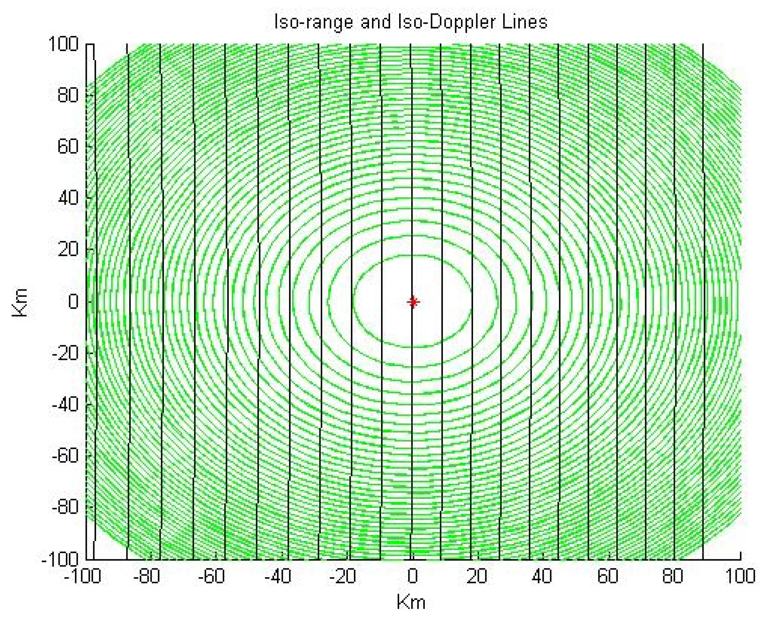In the rough surface case, the signal power in a GNSS return at the specular reflection point will include delays up to twice the chipping length on the surface (see [18] for more information). For an illustration of how the GPS L1 C/A code signal spreads across the surface see Figure 1. The de-spreading processing which is performed to recover the GPS

Figure 1. Lines of constant delay and frequency for a GPS L1 reflection received at a 10 degrees incident angle. Constant delay ellipses (green) are at 1 chip intervals (approximately 293 m total path delay), and Doppler parabola spacings (depicted as black straight lines because of the degenerate geometry in this example) are at 100 Hz intervals. Image re-used with permission from [18].

Figure 1. Lines of constant delay and frequency for a GPS L1 reflection received at a 10 degrees incident angle. Constant delay ellipses (green) are at 1 chip intervals (approximately 293 m total path delay), and Doppler parabola spacings (depicted as black straight lines because of the degenerate geometry in this example) are at 100 Hz intervals. Image re-used with permission from [18].

signal, effectively mixes waveforms from adjacent code delay chips. In the case of the first iso-range ellipse, the processed signal waveform from the second delay ellipse will contribute to the waveform of the first delay bin, thus making any clear separation of the surface areas problematic.

Another difference with most traditional radar remote sensing instruments is the bistatic geometry and the combination of coherent and non-coherent integration. The normal coherent integration time for a GNSS signal is 1 ms, which is required to recover the signal from below the noise floor. Additionally, non-coherent averaging of consecutive coherent 1 ms waveforms to mitigate the affects of speckle noise. This non-coherent averaging is often performed over intervals of upto and over 100 ms [23]. This necessary averaging degrades the measurements resolution as the signal is averaged across the surface. The coherent integration time of 1 ms corresponds generally to a 1,000 pulse repetition frequency (PRF), and assuming 100 averaged looks, the signal will travel approximately 0.75 km for an 800 km Low Earth Orbit satellite. This gives a rough estimate of the achievable along track resolution of a GPS reflection, although shorter averaging intervals can be used, as shown below. Notably, most of the signal power will be returned in a limited region in the vicinity of the specular reflection point.

The measurements where collected with a large footprint relatively low gain antenna [27], which covered the entire glistening zone in most cases (e.g., these signals where not antenna bandwidth limited). The total surface area where power is received is dependent on the surface roughness and can cover 10’s of square kilometers [24]. Over this area, the signal is mapped over the surface using delay and Doppler

Table 1. Values of the predicted and detected GPS L1 code phases (in chips) for the February 4th 2005 ice reflections.

Signal	sec 1	sec 2	sec 3	sec 4	sec 5	sec 6	sec 7
Direct Calculated	776.8	769.8	762.8	755.7	748.6	741.5	734.3
Direct Observed	776.0	769.5	763.0	756.0	749.2	742.5	734.6
Reflected Calculated	919.3	913.8	908.3	902.8	897.3	891.7	886.1
Reflected Observed	918.5	913.5	908.0	903.0	897.8	892.0	886.0

Table 1. Values of the predicted and detected GPS L1 code phases (in chips) for the February 4th 2005 ice reflections.

Signal	sec 1	sec 2	sec 3	sec 4	sec 5	sec 6	sec 7
Direct Calculated	776.8	769.8	762.8	755.7	748.6	741.5	734.3
Direct Observed	776.0	769.5	763.0	756.0	749.2	742.5	734.6
Reflected Calculated	919.3	913.8	908.3	902.8	897.3	891.7	886.1
Reflected Observed	918.5	913.5	908.0	903.0	897.8	892.0	886.0

(as depicted in Figure 1). The only unambiguous point is the specular reflection point, and the movement of this point during the integration interval will limit the surface resolution.

Initial models have demonstrated that the power return profile can be reasonably determined in the open ocean case using an estimation of the surface slope distribution (i.e., surface roughness) [25].

3.3. Detecting the Reflected Signal

The data shown in Section 4 was sampled at an intermediate frequency, downloaded to the ground and processed with a custom software receiver. Details of the sampled signal can be found in this open source processing tool [18]. The software included in was modified to perform signal detection and tracking as described below.

Initially, the signal is located in Doppler frequency and code delay using pre-calculated estimates based on the receiver and transmitter locations and clock errors. The receiver location and clock state was calculated using the on-board GPS receiver navigation packet and the GPS satellite positions were calculated using orbit and clock data provided by the International GNSS Service (IGS) [26]. The calculation of the signal specular reflection point on the surface is derived in Appendix A of this paper, with example code available on the Internet [18]. The Doppler frequency and code phase calculations are provided in Appendix B and Appendix C, respectively.

The estimated code phases for both the direct and reflected signals are listed in Table 1 for the February 4th reflection. As can be seen in both cases the estimated and detected code phases consistently match to within a single code phase chip (or about 293 meters). The detected code phases are approximate as the peak of the signal is not tracked in the traditional sense, but open-loop tracked as described below. This loosens the accuracy on forward predicting the code phase as the signal is normally processed at a wide range of delays around a reference. After the initial estimation and detection, it is possible to close-loop track the signal using a comb of correlators around an initialized window. Details of this process are described below, which enables real-time code tracking of surface reflections.

The Doppler frequencies of the direct and reflected signal for the February 4th signal are shown in Table 2. As in the case of the code phase detection, the detected Doppler frequency is only coarsely determined. The frequency bandwidth of a GPS C/A code signal is 1000 Hz which allows for reasonable errors in the frequency estimation. The frequency response of the reflected signal is an area in need of further study for the case of ice reflections. Previously, the signal frequency spreading has been shown to be a good indicator of the ocean surface roughness and may prove to be a useful parameter in sensing the ice roughness [27].

Table 2. Values of the predicted and detected Doppler frequencies for the February 4th 2005 ice reflections.

Signal	sec 1	sec 2	sec 3	sec 4	sec 5	sec 6	sec 7
Direct Calculated	–12,042	–12,098	–12,153	–12,208	–12,263	–12,317	–12,372
Direct Observed	–12,040	–12,100	–12,080	–12,280	–12,300	–12,260	–12,380
Reflected Calculated	–9,819	–9,863	–9,907	–9,950	–9,994	–10,037	10,081
Reflected Observed	–9,720	–9,600	–9,680	–9,740	–9,820	–9,900	–9,920

Table 2. Values of the predicted and detected Doppler frequencies for the February 4th 2005 ice reflections.

Signal	sec 1	sec 2	sec 3	sec 4	sec 5	sec 6	sec 7
Direct Calculated	–12,042	–12,098	–12,153	–12,208	–12,263	–12,317	–12,372
Direct Observed	–12,040	–12,100	–12,080	–12,280	–12,300	–12,260	–12,380
Reflected Calculated	–9,819	–9,863	–9,907	–9,950	–9,994	–10,037	10,081
Reflected Observed	–9,720	–9,600	–9,680	–9,740	–9,820	–9,900	–9,920

3.4. Tracking the Reflected Signal

The signals above are both easily trackable in real time using both open-loop and closed-loop methods. The key to tracking the signal is predicting narrow delay and Doppler windows by using the reflection geometry and IGS satellite and clock information. Currently, the IGS provides satellite location information propagated into the future for 24 hours, which could be uploaded daily to a space based instrument. Additionally, the clock biases of the GPS satellites are very stable and can be propagated into the future relatively easily and accurately.

The Doppler frequency of the reflected signal changes slower than the code delay and the signal can be reasonably centered in frequency using the calculations shown in Appendix B at a rate of once per second. The reflected signal can be tracked using a number of different methods, a few of which are described below.

Open-Loop Signal Tracking 

The easiest way to open-loop track the signal is with a correlator “net” as shown in Figure 9 and Figure 11. In this case correlators were space around a pre-predicted code delay center at 1/10 chip steps over a window approximately 4 chips wide. This spacing and window is more than would normally be needed but allows for the easy application of bounding or centering logic to run in the background.

After the initial code delay estimation the signal can be open loop tracked based on the code delay rate of change only. Centering the correlators on the predicted absolute value of the code delay is also very reliable. In both cases care needs to be taken to account for gaps in the receiver navigation solution. The center of the open loop tracking correlators is adjusted at each millisecond based on the predicted change in the delay of the reflected signal as follows,

$$\Delta \varphi =\frac{{\varphi }_{reflected}^t-{\varphi }_{reflected}^{t-\Delta t}}{\Delta t}$$

(1)

Additionally, as each interval is processed and the signal looks averaged, it is useful to sequentially store the signal maximum code delays. This maximum will not provide a stable tracking point (as it tends to jump slightly between intervals in an occasionally unpredictable manner), but it will provide a reasonable center bin "anchor" for the correlator net.

Closed-Loop Signal Tracking 

For the case of closed loop tracking the signal’s maximum bin can be used as the reference for a prompt tracking correlator, but with the understanding that due to the signal spreading in delay it will not lie exactly at the surface specular point. The two signals shown above were successfully closed loop tracked using a standard early-minus-late GPS C/A code discriminator. However, the tracking loop requires a longer averaging interval (for example, 100 ms) to better mitigate fading noise and insure a signal peak is present between the early, prompt and late correlators. Additionally, it is useful to add a couple of checks on the error corrections to prevent spurious code adjustments outside the predicted signal window. These checks can be calculated as quickly as processing overheads will allow and include:

• If the delay correction is greater than 1/2 chip, do not adjust prompt correlator and wait for next measurement interval.
• Every second or less, check for the minimal presence of a signal above a pre-calculated noise floor.
• Every second verify the prompt tracking bin is within a reasonable tolerance of the predicted code delay.

However, closed-loop tracking is not recommended for an on-board real-time system. This is partially due to the fact that on-board processing capabilities exist that enable robust open loop methods. It must be kept in mind that in traditional GPS receivers, closed loop tracking is essential due to the random motion of most receivers (in cars, etc.). For a GNSS remote sensing instrument, it is usually assumed that the instrument or vehicle already has a GNSS receiver for navigation. Therefore, the receiver location and GPS time are usually known to high accuracy, and the reflected signals can be treated as independent measurements with no intent to navigate. This generally results in the open-loop tracking methods being much more convenient and robust for an on-board real-time configuration. Notably, In the field of atmospheric sensing using GNSS occultations, it is often the case that the signals are open-loop tracked as the satellites rise and set through the atmosphere [28].

4. Experimental Data

The first step in determining the feasibility of this technique was to perform a coarse validation using two raw data collections from the GNSS reflections experiment on-board the UK-DMC satellite. In 2005, two short duration data sets were collected over sea ice. The data sets were collected on February 4th and June 23rd 2005, over the Bering Sea and off the coast of Antarctica, respectively. Details of the signals detected and in-situ co-located estimates for these data sets are presented below. The specular reflection locations were estimated as follows: the February 4th data collection traveled between approximately [59.09 N, 162.85 W] and [58.74 N, 163.13 W]; the June 23rd signal traveled between [64.29 S, 1.76 W] and [63.83 S, 2.07 W] over the duration of their respective collection intervals.

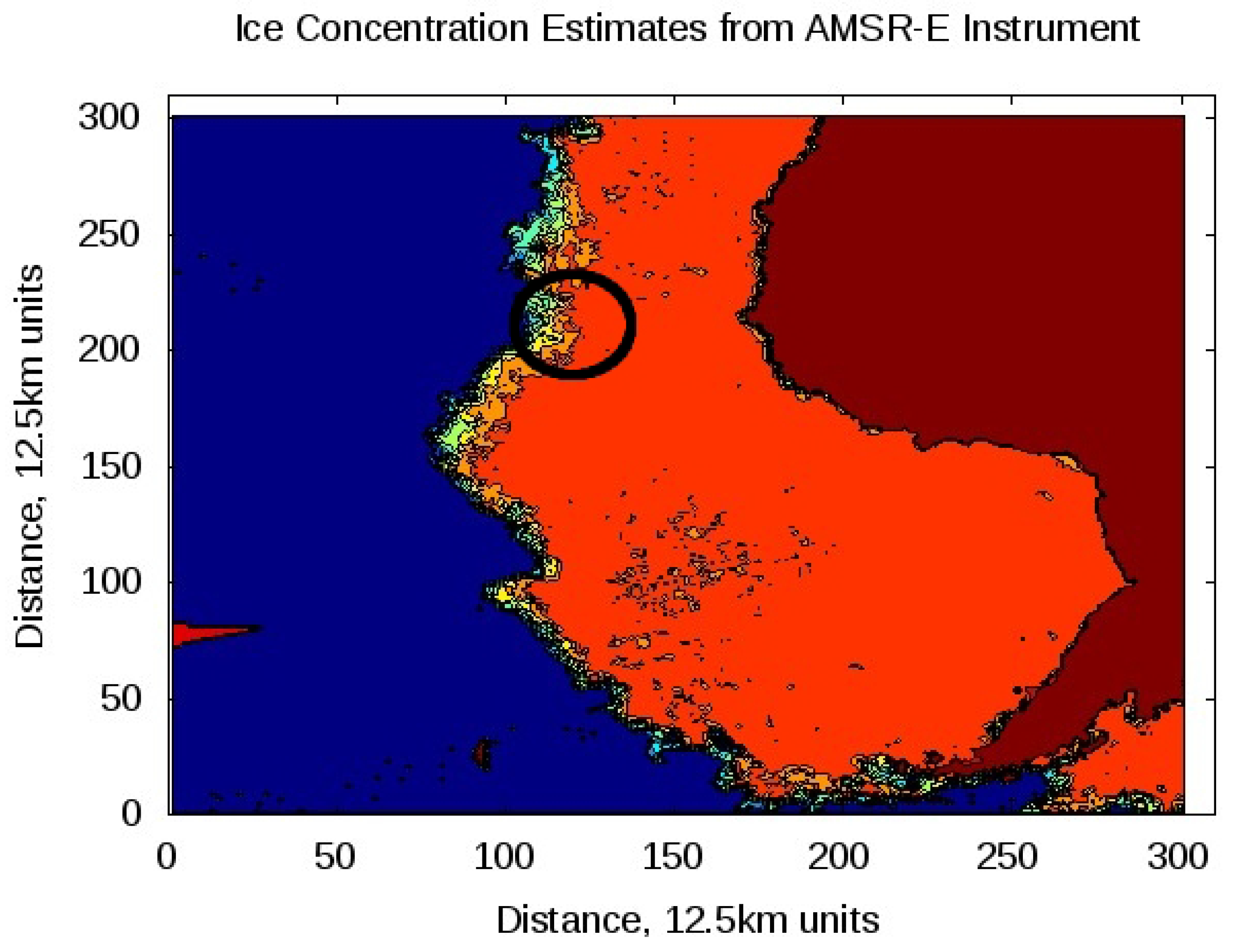
Figure 2. Data from the AMSR-E instrument on the Aqua satellite for February 4, 2005. Including total ice concentration over the collection region. The greater collection region is circled in black, where the reflection moved over areas of ice concentration between 96 and 91 percent. Dark blue represents ocean, increasing ice concentration changes from blue to dark orange and land is shown in brown. The National Ice Center charts indicated the entire collection interval was from 90 to 100 percent ice.

Figure 2. Data from the AMSR-E instrument on the Aqua satellite for February 4, 2005. Including total ice concentration over the collection region. The greater collection region is circled in black, where the reflection moved over areas of ice concentration between 96 and 91 percent. Dark blue represents ocean, increasing ice concentration changes from blue to dark orange and land is shown in brown. The National Ice Center charts indicated the entire collection interval was from 90 to 100 percent ice.

4.1. Independent Co-located Sea Ice Information

Estimates of the ice surface at the time of the two data collections were obtained from the National Snow and Ice Data Center [2] and the AMSR-E instrument on board the Aqua Earth observation satellite [1]. The AMSR-E conditions during the collection of the February 4th data set is shown in Figure 2. For the second GPS collection the ice concentrations from AMSR-E at the time of the June 23rd Antarctic data collection is shown in Figure 3. Figure 4 provides AMSR-E ice concentration estimates together with the National Ice Center chart values over the ground track of the GPS reflection.

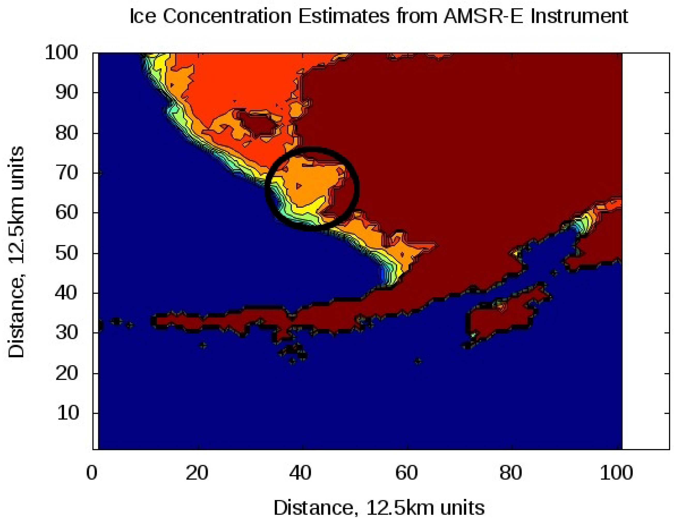
For the February 4th data collection, The values of ice concentration over the collection location ranged between 91 and 96 percent according to AMSR-E data, while the National Ice Center charts indicated the entire collection was within an area of 90 to 100 percent ice concentration (not shown). Conversely, the June 23rd data collection shows changing ice conditions over the collection track. During this collection the satellite was traveling from south to north (or roughly right to left in Figure 3). Initially, the collection starts in an area of 100 percent sea ice concentration, but towards the end of the collection the sea ice concentration begins to decrease according to both AMSR-E and National Ice Center charts.

Figure 3. Data from the AMSR-E instrument on the Aqua satellite for June 23, 2005. Including the total ice concentration over the collection region. The greater collection region is circled in black and the ice concentration over the reflection path is shown in Figure 4. Dark blue represents ocean, increasing ice concentration changes from blue to dark orange and land is shown in brown.

Figure 3. Data from the AMSR-E instrument on the Aqua satellite for June 23, 2005. Including the total ice concentration over the collection region. The greater collection region is circled in black and the ice concentration over the reflection path is shown in Figure 4. Dark blue represents ocean, increasing ice concentration changes from blue to dark orange and land is shown in brown.

4.2. Delay Power Profiles

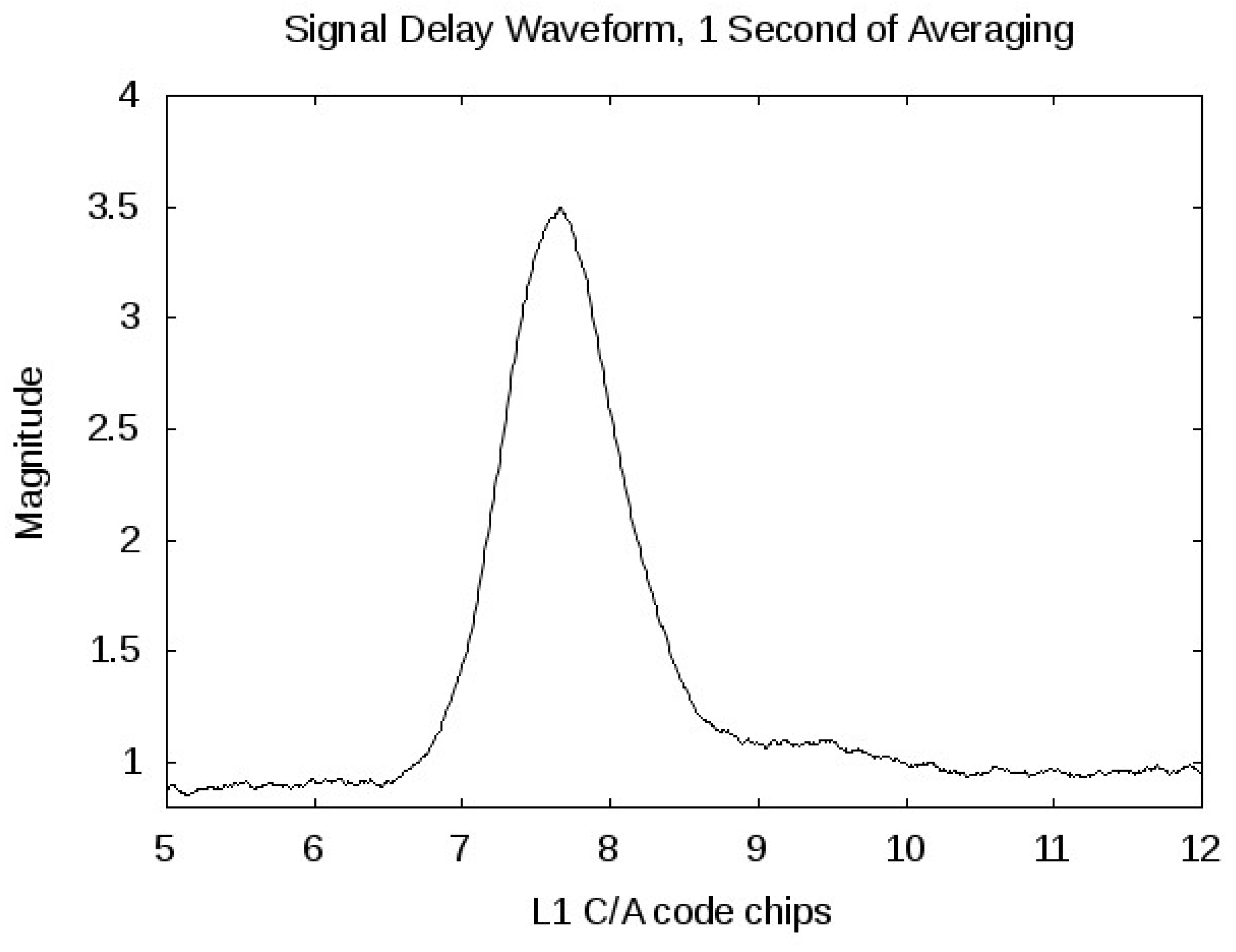
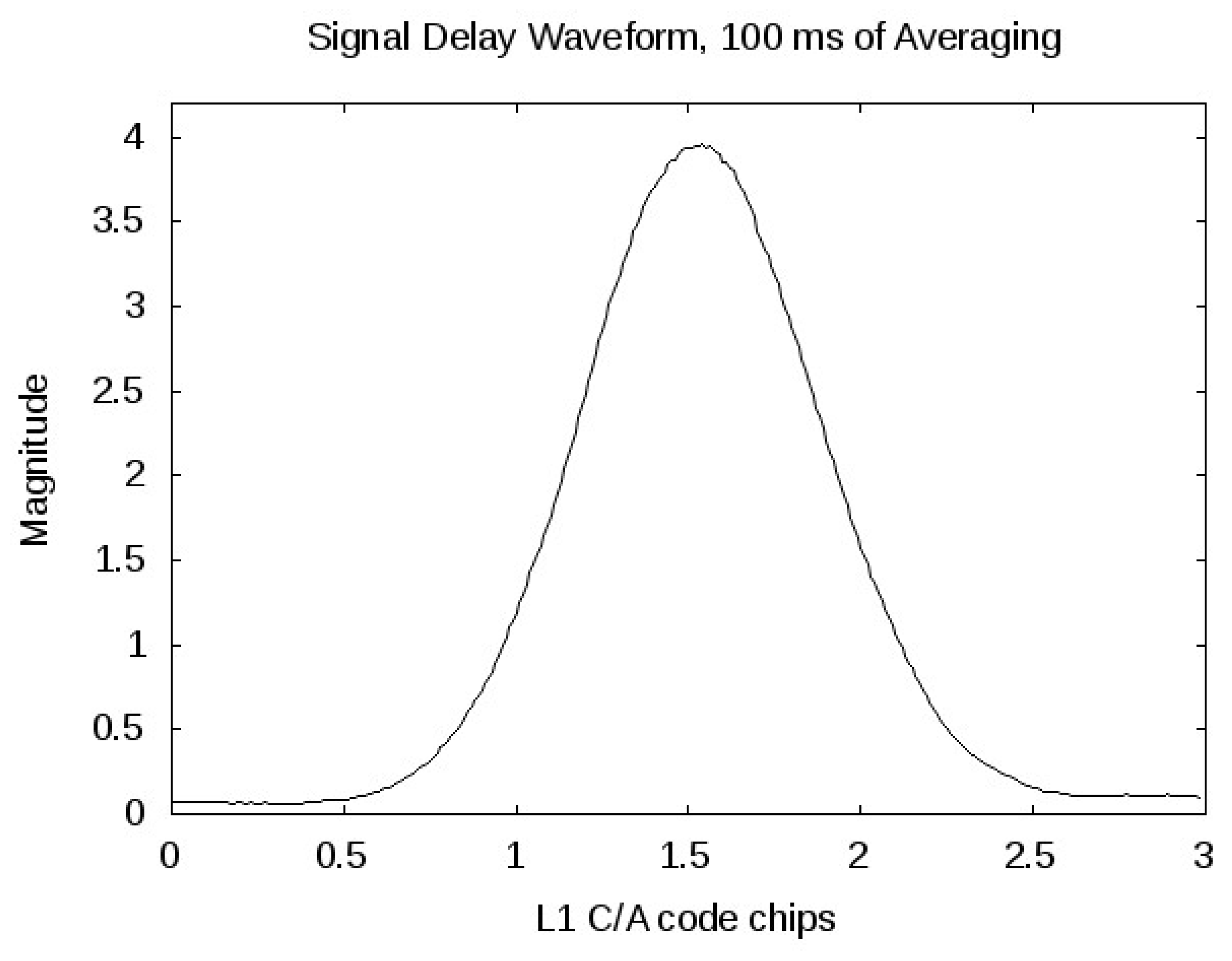
Signal power delay profiles are shown in Figure 5 and Figure 6 for the two ice reflected signals. The first things to notice include; the signal power of the February 4th signal is significantly higher than that of the June 23rd signal and there is a noticeable spreading of the signal across wider delay bins in the June 23rd reflection. The February 4th signal was averaged over 100 ms, while the June 23rd signal was averaged over a complete second to better visualize the signal spreading (note the larger x-axis range in Figure 6). However, the magnitudes are nearly the same despite the significantly longer averaging interval for the June 23rd signal.

The higher power returns received on February 4th are interesting, given that the ice concentration maps indicate that both reflection start in an area of high ice concentration. It could be that the ice surface roughness is playing a significant role in determining the scattered signal power. It may be the case that there is an intermittent coherent component in the February 4th signal. This would be evidence that the ice from which this signal was reflected was very smooth (based on the Rayleigh roughness criterion for an incident wavelength of approximately 19 cm). However, a signal containing even a trace of coherency would greatly increase the processed signal levels and strongly suggests that the ice surface and any water present within the reflection footprint was very smooth.

These signal return magnitudes are not radar cross section measurements. Parameters such as the free space path loss, transmit power, transmit and receive antenna gains and reflection angle have not been

Figure 4. Ice concentration estimates from AMSR-E and National Ice Center charts over the path of the specular reflection point for June 23, 2005 data. The two vertical lines are the approximate start and end points for the GPS reflection (reflection traveling from right to left, covering approximately 53 km). The AMSR-E data is shown as the black trace, starting at 0 on the far left (open sea) and progressing upwards to 100 ice concentration towards the right. The National Ice Center concentrations of 70 to 80 percent and 90 to 100 percent are shown as orange and red shaded areas, respectively.

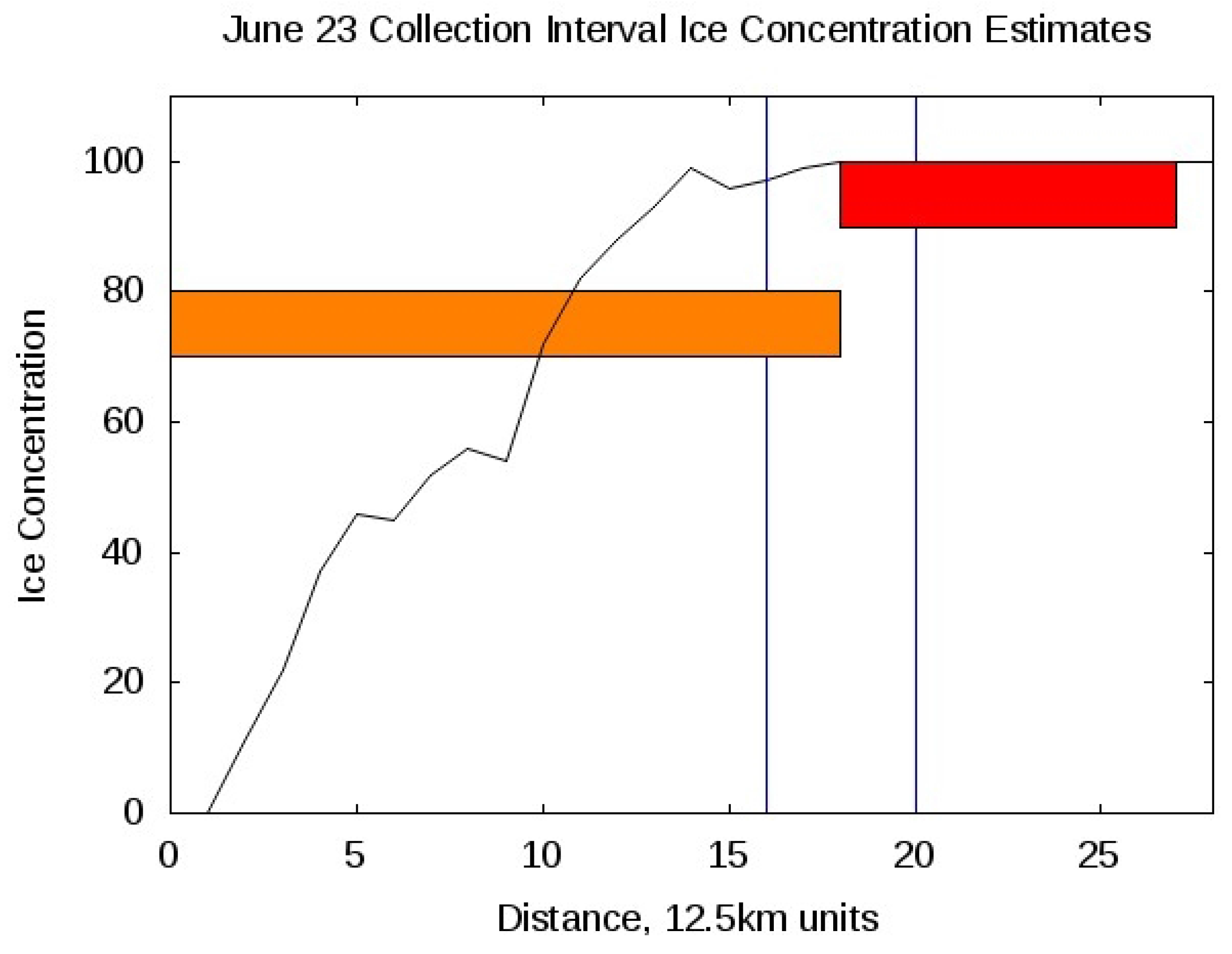
Figure 4. Ice concentration estimates from AMSR-E and National Ice Center charts over the path of the specular reflection point for June 23, 2005 data. The two vertical lines are the approximate start and end points for the GPS reflection (reflection traveling from right to left, covering approximately 53 km). The AMSR-E data is shown as the black trace, starting at 0 on the far left (open sea) and progressing upwards to 100 ice concentration towards the right. The National Ice Center concentrations of 70 to 80 percent and 90 to 100 percent are shown as orange and red shaded areas, respectively.

corrected for. However, the difference in signal power between the two signals is an order of magnitude which is beyond the contribution of all the above mentioned factors combined.

The power returned at delays several chips removed from the specular reflection point on June 23rd suggest a rougher ice surface, possibly due to a higher concentration of older first-year, second-year or multi-year ice (see increased level near chip 9 in Figure 6). The signal spreading could also be caused by the presence of rough water in the reflection footprint (which would cover approximately 40 km square in this case), which is directly related to the ice concentration.

4.3. Signal Variation Over Collection Interval

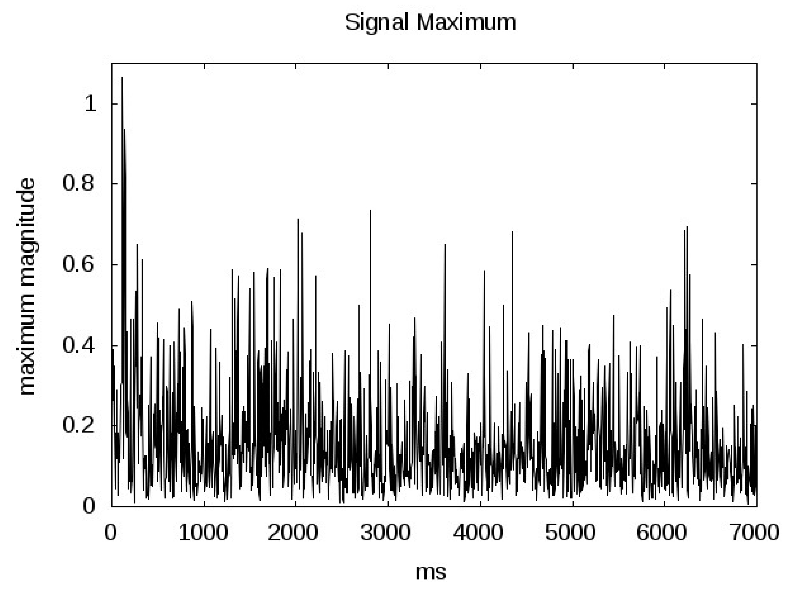
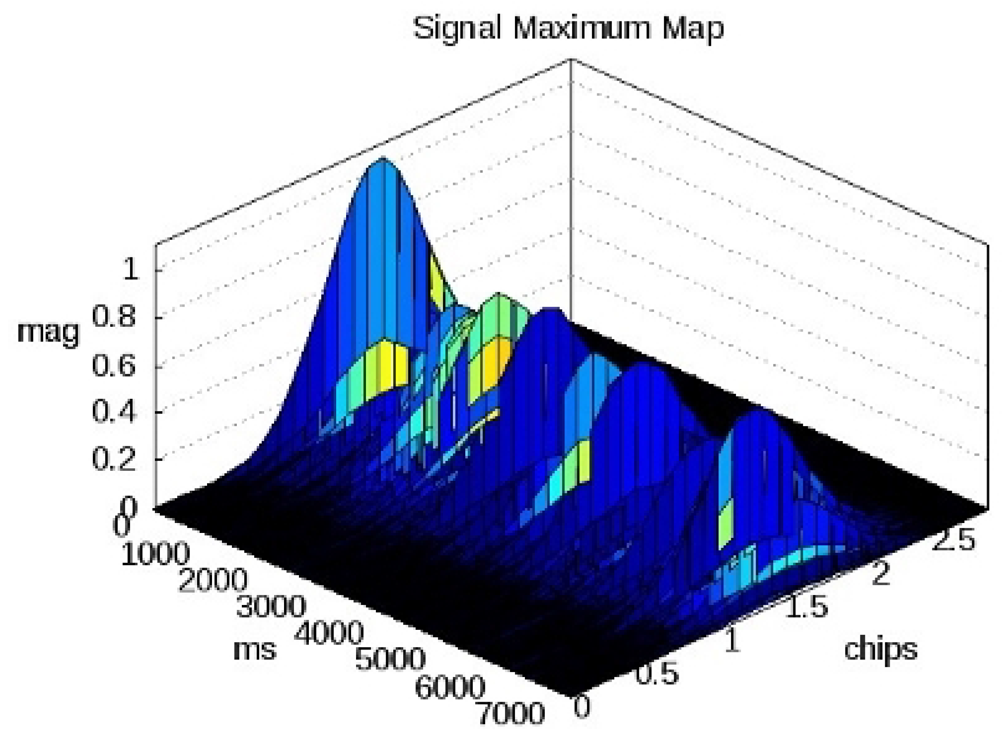
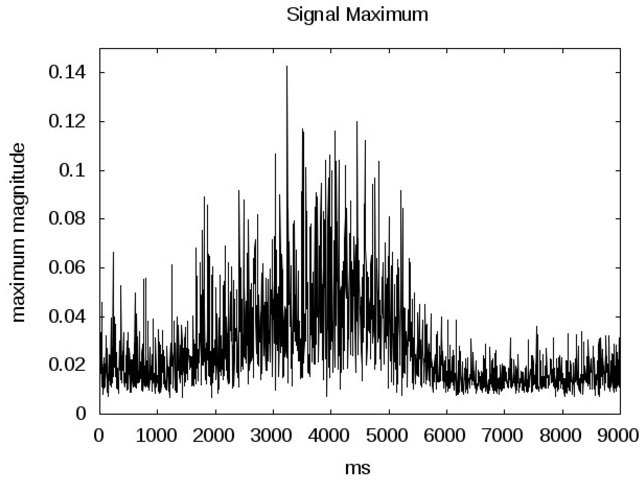
Figure 7 and Figure 8 show the signal magnitude variation over the collection intervals for both signals. In these plots the signals were averaged over only 5 ms. The February 4th signal clearly has a greater magnitude than the June 23rd signal. Additionally, the June 23rd signal reveals fluctuating magnitudes over the collection interval. In this case, the GPS reflection shows lower returns at the start of the collection which gradually increase between seconds 2 and 6 and end in an abrupt decrease in the power returned towards the end of the collection interval. At this point in the collection both AMSR-E and National Ice Center data reveal changing ice conditions (although less drastic in the AMSR-E data).

Figure 5. An example power delay for February 4th 2005 signal. The x-axis is in GPS L1 C/A code chips and the y-axis is the total accumulated signal power after 100 ms of non-coherent averaging. For an example of how chip delays map to the surface, see Figure 1.

Figure 5. An example power delay for February 4th 2005 signal. The x-axis is in GPS L1 C/A code chips and the y-axis is the total accumulated signal power after 100 ms of non-coherent averaging. For an example of how chip delays map to the surface, see Figure 1.

Figure 6. An example power delay for June 23rd 2005 signal. The x-axis is in GPS L1 C/A code chips and the y-axis is the total accumulated signal power after 1 second of non-coherent averaging. For an example of how chip delays map to the surface, see Figure 1.

Figure 6. An example power delay for June 23rd 2005 signal. The x-axis is in GPS L1 C/A code chips and the y-axis is the total accumulated signal power after 1 second of non-coherent averaging. For an example of how chip delays map to the surface, see Figure 1.

Figure 7. Signal maximums for the February 4th signal. Signal averaged over 5 ms across entire duration of the data collection. The total surface travel distance over this interval is approximately 42 km.

Figure 7. Signal maximums for the February 4th signal. Signal averaged over 5 ms across entire duration of the data collection. The total surface travel distance over this interval is approximately 42 km.

Figure 8. Signal maximums for the June 23 signal. Signal averaged over 5 ms across entire duration of the data collection. The total surface travel distance over this interval is approximately 53 km. Millisecond 0 corresponds to the higher AMSR-E estimated sea ice concentration and millisecond 9000 to the lower sea ice concentration (See Figure 4).

Figure 8. Signal maximums for the June 23 signal. Signal averaged over 5 ms across entire duration of the data collection. The total surface travel distance over this interval is approximately 53 km. Millisecond 0 corresponds to the higher AMSR-E estimated sea ice concentration and millisecond 9000 to the lower sea ice concentration (See Figure 4).

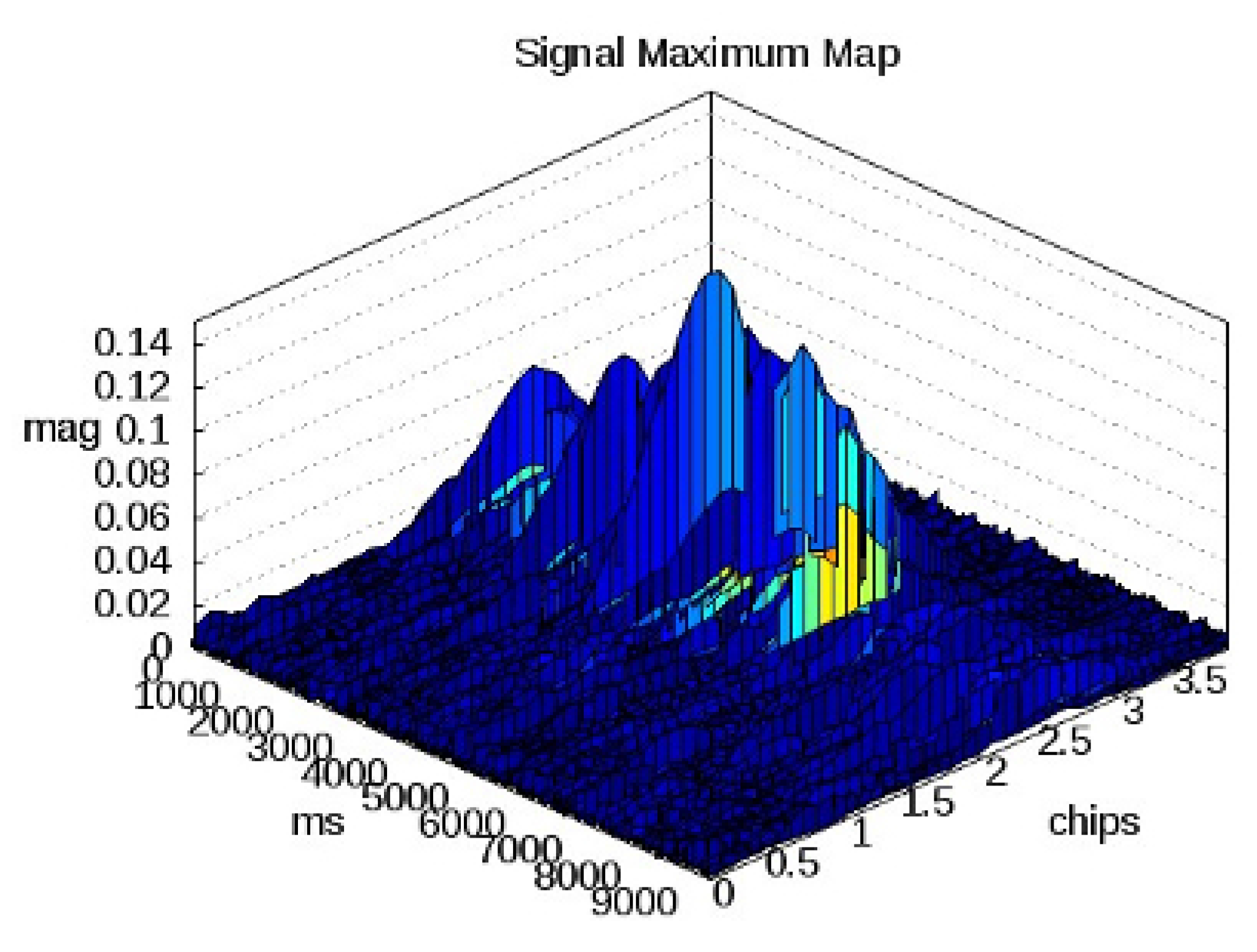
Figure 9. Delay waveform over 7 seconds for the February 4th 2005 reflection event.

Figure 9. Delay waveform over 7 seconds for the February 4th 2005 reflection event.

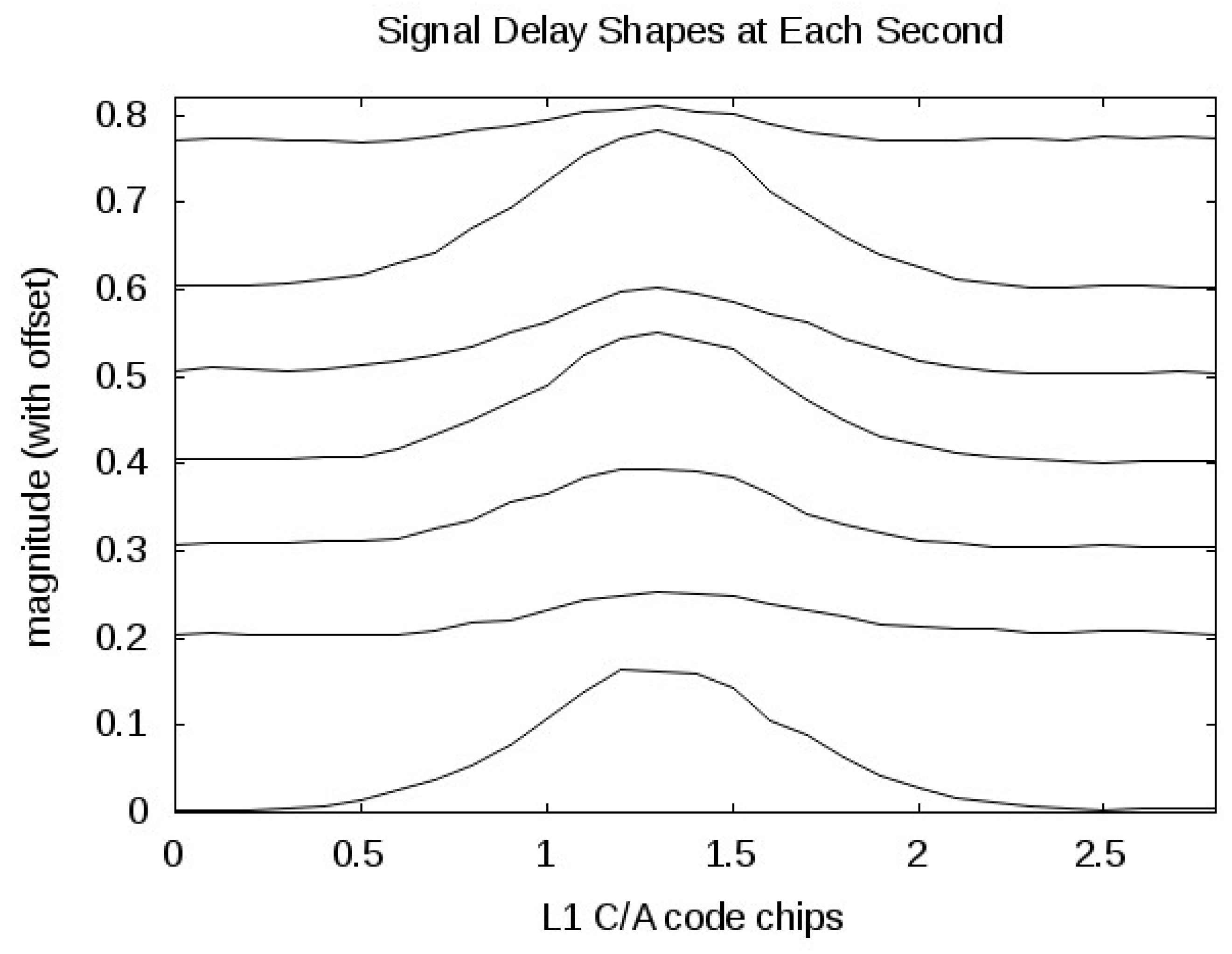
Additional details can be observed by looking at the signal delay shape across the collection interval. Figure 9 through 12 show the same signal averaged over 5 ms intervals (5, 1 ms looks) and the resulting power returns over time. First as a 3-D image in time, delay and magnitude and then as a second 2-D stack across the event interval (with consecutive seconds offset vertically for clarity). Averaging over only 5 looks results in both signals exhibiting sharp fluctuations, which could be due to signal fading or changing surface conditions across the averaging interval [15]. However, by processing the signal in this way a couple of subtle details are discernible. First, the shape of both signals in the delay dimension contain discontinuities across the minimal 2 chip spreading interval (more evident in the June 23rd signal). The signals are clearly not the rounded peaks over 2 chips as would be the case for a directly detected GPS L1 signal (without any surface reflection). This might indicate the presence of multiple surface reflections mixing across the first two (or more) delay bins. Even in the cases of a strong reflection off a smooth surface, the original signals coherent carrier phase is not completely recoverable, and hence, recovery of the transmitted carrier phase is not possible in nearly all cases for signals received in space.

Also visible in greater detail in Figure 11 is the abrupt transition to a different ice surface at roughly second 7 for the June 23 signal. The exact location of this transition occurs at what seems to be a distinct “edge" which is revealed more clearly with the shorter averaging interval. Interestingly, the National Ice Center data reveals a change to 70 to 80 percent ice concentration at the same point, while the AMSR-E data shows this as the point where the ice concentration begins to decrease. This demonstrates that the GPS measurements are consistent with the National Ice Center ice concentration charts. Although they do not show the more gradual drop off in concentration that the AMSR-E measurements estimate, the change that occurs at that point is being responded to in both cases.

5. Conclusions

This paper provides a preliminary demonstration of how using reflected GPS signals received on-board an orbiting satellite may hold the potential to sense sea ice. The availability of only two

Figure 10. February 4th delay waveforms at consecutive seconds (1 seconds slices of the 3-D image in Figure 9). The waveforms are arbitrarily offset for clarity, where second 0 is plotted at the lowest offset and subsequent seconds are plotted with increasing offsets.

Figure 10. February 4th delay waveforms at consecutive seconds (1 seconds slices of the 3-D image in Figure 9). The waveforms are arbitrarily offset for clarity, where second 0 is plotted at the lowest offset and subsequent seconds are plotted with increasing offsets.

Figure 11. Delay waveform over 9 seconds for the June 23 2005 reflection event.

Figure 11. Delay waveform over 9 seconds for the June 23 2005 reflection event.

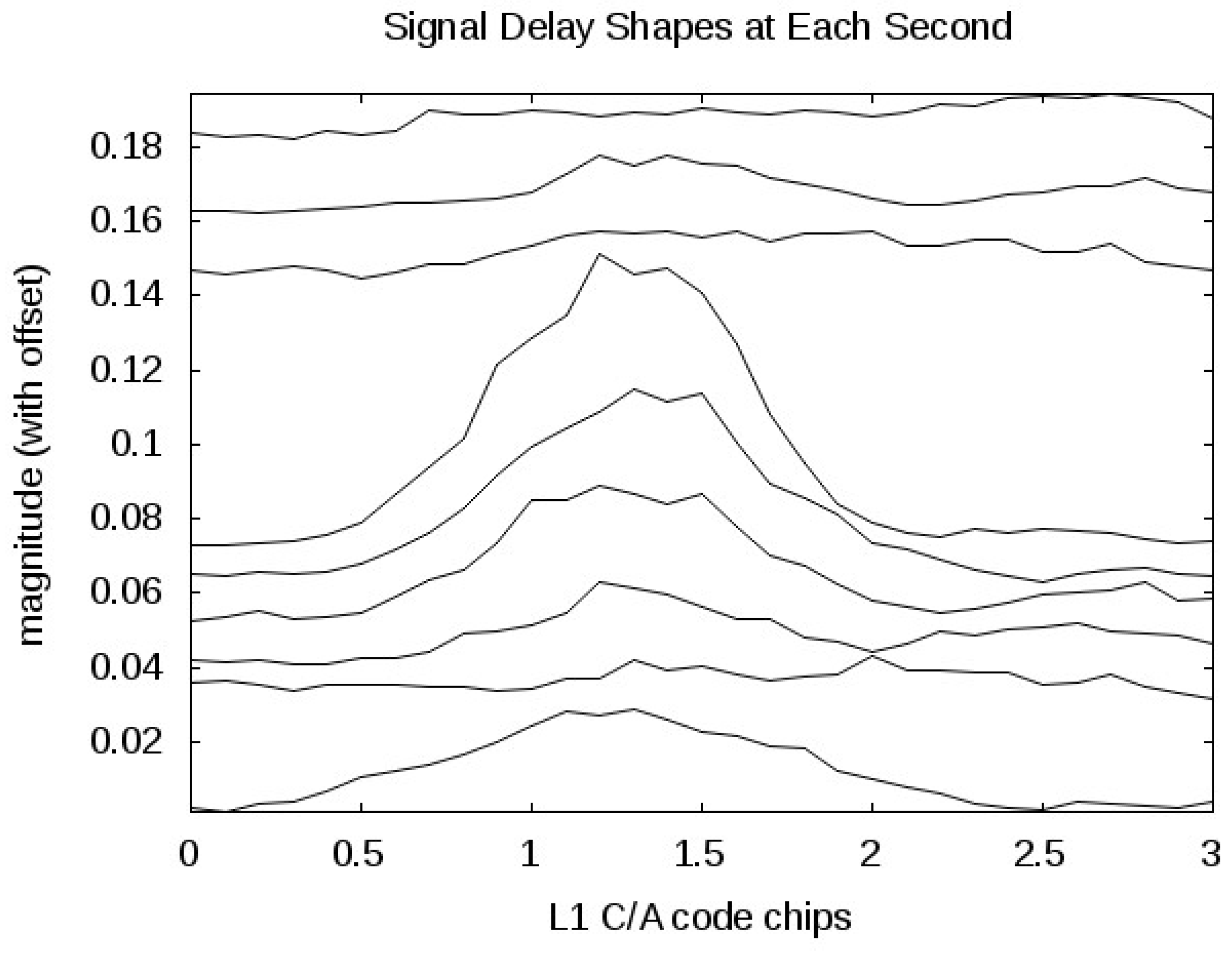
Figure 12. June 23 delay waveforms at consecutive seconds (1 seconds slices of the 3-D image in Figure 11). The waveforms are arbitrarily offset for clarity, where second 0 is plotted at the lowest offset and subsequent seconds are plotted with increasing offsets.

Figure 12. June 23 delay waveforms at consecutive seconds (1 seconds slices of the 3-D image in Figure 11). The waveforms are arbitrarily offset for clarity, where second 0 is plotted at the lowest offset and subsequent seconds are plotted with increasing offsets.

data sets limits the number and certainty of any conclusions that could be drawn about what is being sensed and to what accuracy. This demonstration strongly illustrates the potential of this technique and its prospects for the future.

However, currently there are several instruments that provide daily sea ice data sets to the research community. What GNSS measurements could provide in addition to this is a legitimate question. One possible answer, suggested but not proven here, is relatively high along track resolution that could provide improved geo-location at points of changing sea ice conditions. Unfortunately, the above datasets do not include a sea ice to ocean boundary, so how accurately the sea ice extent could be determined with this technique is unknown. The other compelling reason to pursue this technology is as a backup to the larger more sophisticated instruments. It is unrealistic to believe this technique will provide measurements on a par with RADARSAT or other similar sensors. However, having alternatives and backups is always a good policy towards insuring continuity and to mitigate the risk should we lose any of the existing or planned future missions for whatever reason.

The biggest practical advantages of a GNSS instrument are simplicity and cost. It relies on "signals of opportunity" transmitted continuously by satellite navigation system constellations, and does not require expensive signal generators and transmitters. The instrument itself can consist of as little as an antenna, an RF down converter and a software receiver, as was used to collect and process the measurements shown above. With the appropriate antenna, it would be possible to detect and track several measurements from a single instrument at different surface locations.

Lastly, an advantage that will emerge as the new generation of GNSS satellites come on-line includes the transmission of additional frequencies. The signals above where all from the GPS L1 L-band signal. The new constellations will transmit publicly available codes at 3 separate L-band frequencies which should prove useful additions into the existing methods of satellite based sea ice sensing.

On the other hand, the disadvantages include: the navigation ranging code which spreads the received waveforms between adjacent delay bins, the very weak signal transmit levels which necessitate a coherent processing interval on the order of 1 ms [23] and the variability of specular reflection locations on the surface. The measurement locations will consist of arcs between the receiving and transmitting satellites and often do not provide 100 per cent coverage over a given area, but a gradual filling in over several orbits. It is thought that with suitable instrument configurations and creative processing strategies, these difficulties can be sufficiently mitigated.

Generally, GNSS-R is an interesting technique which holds a promising future in many areas of environmental remote sensing. It is believed that the measurements provided by a GNSS bistatic instrument can be incorporated into the existing ice sensing systems such as those provided by the National Ice Center [2] or the Canadian Cryospheric Information Network [29]. Using a combined and complimentary strategy holds the most promise for GNSS measurements to contribute alongside the existing more established technologies used to sense the Earth’s sea ice.