1. Introduction
Estuarine areas and rivers are very complex and dynamic systems. Areas around these rivers and estuaries are often populated and can serve as important shipping channels, which implies erosion and pollution by toxins. The latter is transported by Suspended Particulate Matter (SPM), which is highly concentrated in estuaries. Knowing SPM loads and its spatial distribution is therefore essential in maintaining and controlling these environments.
SPM is one of the three main optically active constituents in natural waters. The other optically active constituents are Chlorophyll (CHL) and Colored Dissolved Organic Matter (CDOM). Since these constituents affect the color of the water, it is possible to detect their presence in water using remote sensing and quantify their respective concentrations [
1]. Pure water itself has a blue color, but, with an increase of suspended sediments, the water turns, in most cases, brown due to the stronger absorption in the blue and the strong backscattering in the visible and near infrared part of the electromagnetic spectrum [
2]. CHL will add a green color to the water by absorbing blue and red light and CDOM contributes a yellow-brownish color because of the high absorption in the blue. These findings always relate to surface concentrations since the water penetration depth is limited (~1 meter or less in highly turbid water for red and near-infrared wavelength region).
Estuarine and coastal waters are, however, complex in their composition and optical properties. Therefore, relatively simple global algorithms developed for open oceans are not applicable to these waters. Several authors pointed out the strong regional variations in optical properties for these coastal and estuarine areas and have encouraged the development of algorithms on a regional scale. In [
3] and [
4], absorption and scattering coefficients were measured for different coastal waters (North sea and English Channel, Lions Gulf, Northern Adriatic sea, Baltic). The mass specific scattering coefficient of particles (close to 0.5 m
2/g at 555 nm) and the spectral shape showed considerable variability within each region and on a region-by-region basis. According to [
4], these differences originate from variability in the size distribution and the particle composition. The exponential slope of CDOM varied only slightly around 0.0176 nm
−1. The relationship between phytoplankton absorption and TCHL (the sum of CHL a and phaeopigments) was similar to that previously observed by [
5], but revealed significant variability among the regions. Finally, most absorption spectra of Non-Algal Particles (NAP) could be described by an exponential function with a slope of 0.0123 with weak variations. Likewise, Darecki
et al. [
6] showed that the inherent and apparent optical properties of the Baltic Sea waters are subject to significant seasonal variations, due to the seasonal cycle of hydrological regimes and biological cycles. For the Eastern English Channel, Vantrepotte
et al. [
7] found a pronounced seasonal variation in bio-optical properties with relevant differences between winter and spring-summer periods. For estuarine waters [
8], absorption and backscattering coefficients were in the range observed in [
3] and [
4], but with significant variations within one estuary and between different estuaries.
Despite their complexity, there is a growing interest in the study of estuarine and coastal waters and the development of algorithms to derive total suspended matter from remotely sensed data. Algorithms are empirically, semi-empirically derived, or based on an analytical method. In the analytical approach, the water constituent concentrations are physically related to the measured reflectance spectra using sophisticated radiative transfer models (e.g., Hydrolight) or (semi-) analytical bio-optical models. To determine the water quality parameters (e.g., SPM), these models are inverted through neural networks, matrix inversion [
9] or curve fitting [
10]. This approach requires detailed information about the inherent optical properties (IOP) like the absorption and the backscattering coefficients. As already pointed out, there is a large variety in these optical properties for different coastal and estuarine waters. Therefore care must be taken when applying these analytical models and to derive water quality estimates.
The empirical approach is based on a statistical calibration relationship between spectral data and SPM. The derived relationships are valid only for data having statistical properties identical to those of the training data. Therefore these algorithms are sensitive to changes in the composition of water constituents and they are often developed for one specific region and one specific moment in time. Only a few researchers tested the seasonal portability of their empirical algorithms. Matthews
et al. [
11] performed a limited test for a spring and summer dataset for both the Bristol Channel and the north Norfolk coast. For the north Norfolk coast, SPM concentrations ranged between 2–24 mg/L in May and 1.5–22 mg/L in August. CHL concentrations were recorded between 4.9 μg/L and 16.08 μg/l in May and between 0.94 μg/L and 14.5 μg/L in August. For the Bristol Channel, SPM concentrations ranged between 1.5–24 mg/L in June and 1.5–90 mg/L in September. CHL concentrations ranged between 1.87 and 5.36 μg/L in June and between 0.58 and 2.37 μg/L in September. The authors did not cover the full range of suspended solids concentrations (the authors mention that these would be considerably higher in winter) but they achieved accurate estimations of SPM when applying an algorithm to data collected from the same site later in the year. Doxoran
et al. [
12] proposed an invariant band ratio (850 nm/550 nm) algorithm to retrieve the estuarine sediment dominated waters of the Gironde and the Loire [
13]. Hence there are examples of seasonal portability of these empirical algorithms, but they are scarce. Geographical portability on the other hand is not possible due to geologic diversity of the upland basin, the dynamics of ocean currents, and the variety of residence times that will result in highly varying scattering and absorption properties of SPM [
14].
For the Scheldt River in Belgium, an empirical relationship was already found between SPM concentration and a difference of two near infrared bands [
15]. This relationship was developed for June 2005 using both
in situ and hyperspectral airborne data. The development of such an algorithm enforces the need for adequate
in situ samples for calibration. Gathering such calibration data is, however, a real challenge in dynamic environments such as estuaries and rivers. In tidal estuarine waters, such as the Scheldt, concentrations vary rapidly in space and time. Water samples collected for calibration and/or validation purposes of remote sensing data (e.g., airborne or spaceborne) are therefore only representative if they are taken within a close time span of the overpass of the satellite or airplane (with a maximum delay of 5 to 10 min for the Scheldt River). This implies a serious restriction to the acquisition of a sufficient number of training samples to set up an empirical algorithm. To gather an adequate set of field samples in these circumstances, there is a need for multiple vessels, equipment and personnel making such a field campaign very expensive and operationally complex. A more robust SPM algorithm for the Scheldt would therefore be of great interest to the users’ community since extensive field campaigns are no longer required and one could save upon cost and time.
The objective of this study is to find a seasonally robust SPM algorithm for the Scheldt River near Antwerp in Belgium. The algorithm should be broadly applicable to new datasets without the need for simultaneously gathered in situ samples. In situ measured datasets acquired during different seasons and tidal phases are used to build the algorithm. Validation is performed with hyperspectral airborne datasets acquired in June 2005 and October 2007. Since these datasets were acquired under different atmospheric circumstances, special attention is directed to atmospheric and air/water interface corrections.
2. Site Characterization
The Scheldt River rises in the North of France and flows through Belgium and the Netherlands to finally reach the North Sea. The river is rain-fed and the average discharge varies considerable between summer-autumn (60 m
3/s) and winter-spring (180 m
3/s) [
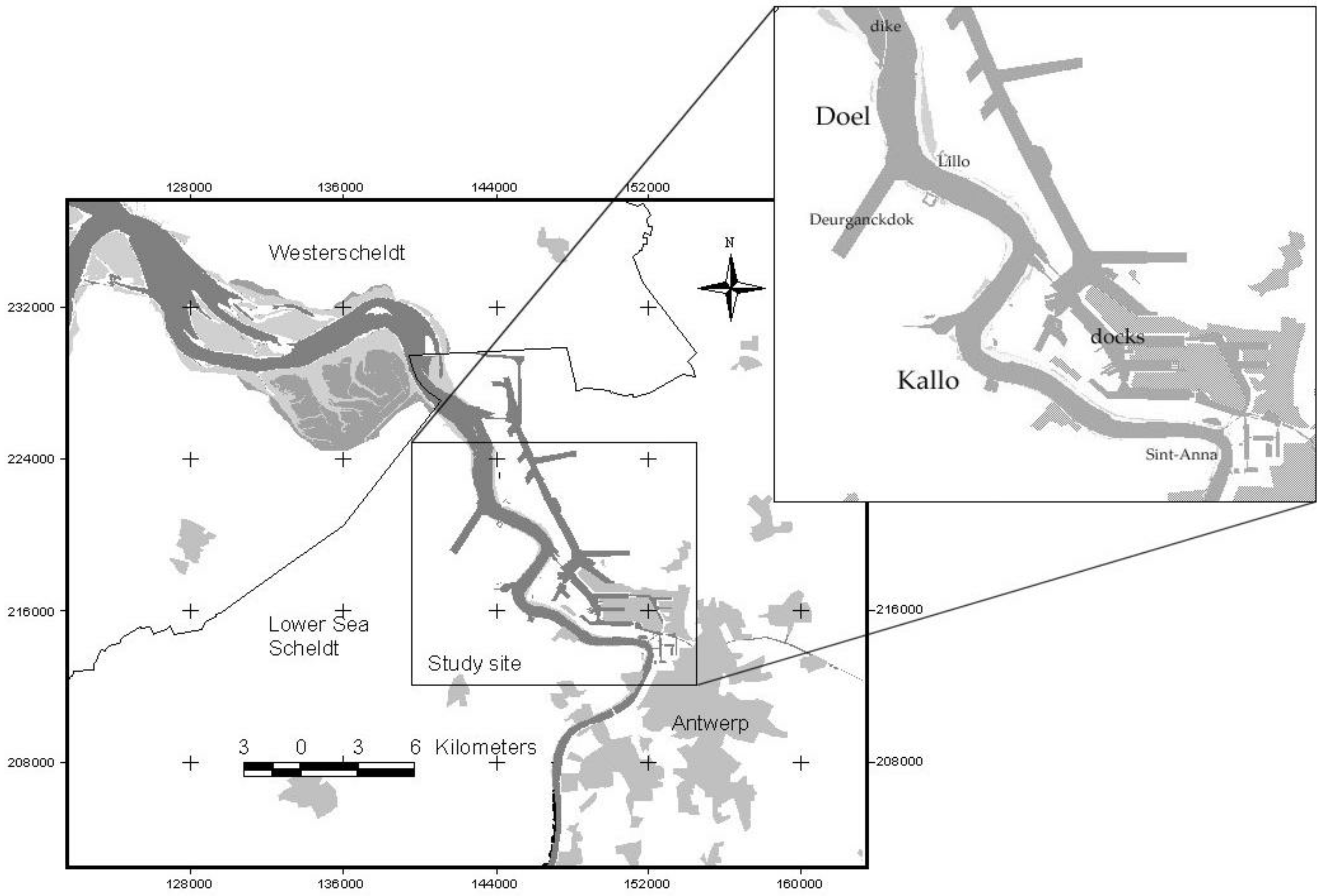
16]. Our study area is part of the brackish lower sea Scheldt, situated between the city of Antwerp (±79 km from the mouth) and the border of Belgium and the Netherlands (±60 km from the mouth) (
Figure 1).
Figure 1.
The Scheldt study site.
Figure 1.
The Scheldt study site.
This zone corresponds to the zone of high turbidity [
16]. Chen
et al. [
17] reported average SPM concentrations of 82 ± 65 mg/L in the uppermost 10% of the water column. However, it has to be noted that these concentrations vary with the tidal cycle and the seasons [
17]. The tide in the Scheldt is semi-diurnal and its influence extends up to Gent, 82 km upstream of Sint Anna (
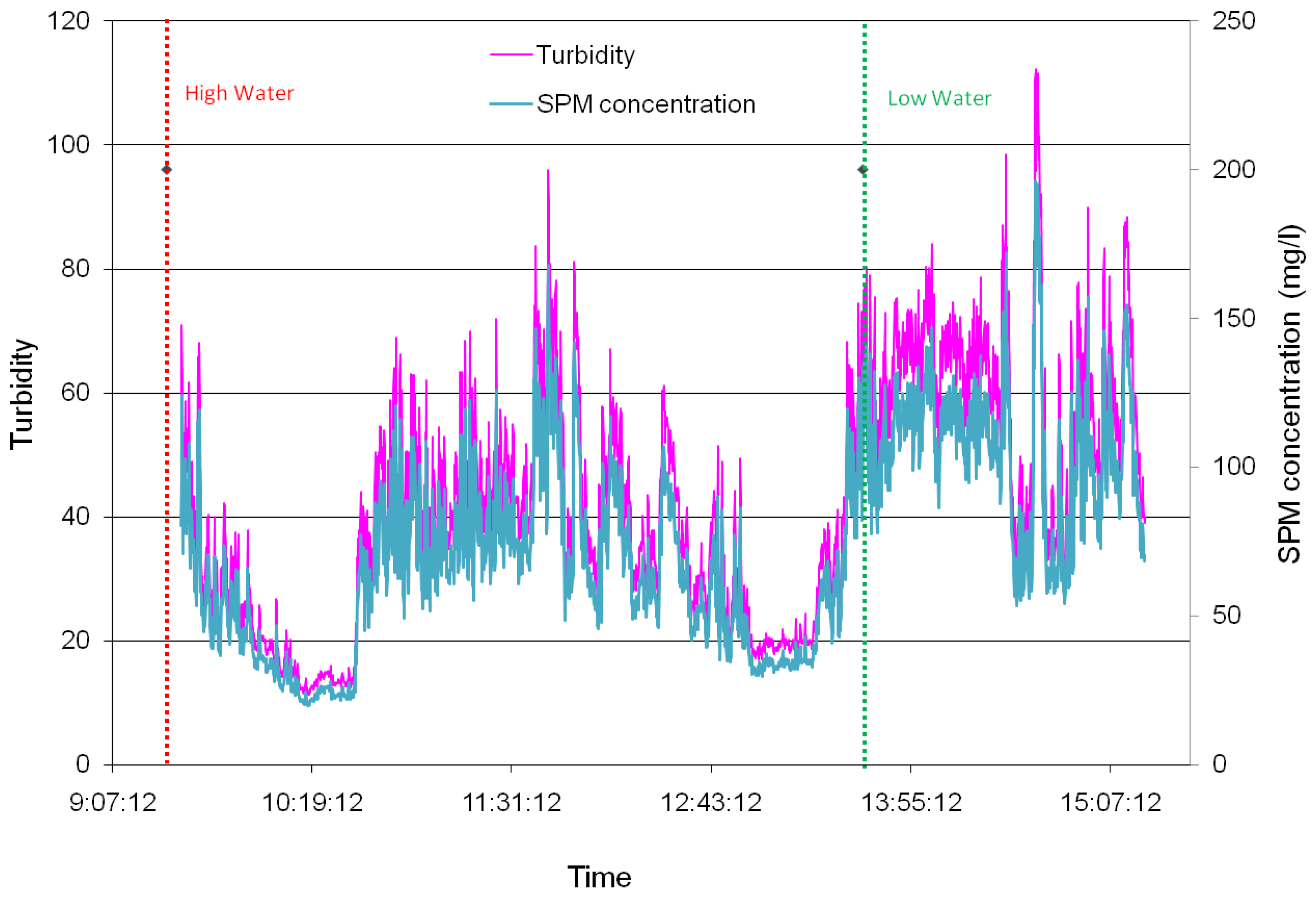
Figure 1). An example of this tidal influence on the surface SPM concentrations is shown in
Figure 2. These data were collected with an OBS turbidity meter mounted in January 2008, 30 cm below the water surface, at pontoon Sint Anna (88 km from the mouth; see the inset in
Figure 1). The measurements started around high water (tide) and ended almost an hour after low water (tide). From these measurements, significant variations can be observed during the tidal cycle. SPM concentrations vary between 30 and 200 mg/L. Small variations with high frequencies can be due to air bubbles, turbulent current variations or local erosion.
The mud found in the Scheldt Estuary is from marine and terrestrial origin. The terrestrial sources are waste water, surface erosion of cohesive soils, erosion of the exposed clay layers at the bottom of the estuary, and precipitation [
18].
Information on the surface CHL and CDOM concentration for the Scheldt study site is rare. In 1996, Muylaert
et al. [
19] reported two phytoplankton blooms for the estuary: one in spring (occurring in the upper estuary >160 km with phytoplankton biomass <100 μg/L), and a second, more intense, in the summer (in the 100–160 km zone). For our study area in particular, concentrations were generally below 10 μg/l with a first slight increase in May–June (concentrations below 20 μg/L) and with a more pronounced increase in August-September (concentrations above 30 μg/L close to Antwerp). For the CDOM concentration, there were some measurements made by [
20] in February 2005 and July 2006 in the Scheldt estuary between the mouth and Antwerp. The authors showed variations in the absorption coefficient of CDOM (aCDOM) at 375 nm between 1.8 and 4.3 m
−1.
Figure 2.
OBS turbidity measurements for pontoon Sint Anna in January 2008.
Figure 2.
OBS turbidity measurements for pontoon Sint Anna in January 2008.
3. Data Collection
To achieve the objectives, a large dataset was set up, consisting of two hyperspectral airborne datasets from the Scheldt River (June 2005 and October 2007), in situ data sampled coincident with the airborne campaigns and extra in situ measurements in 2007 and 2009.
3.1. Airborne Datasets
Two hyperspectral airborne datasets were acquired in June 2005 (spring) and in October 2007 (autumn) at different moments in the tidal cycle (
Table 1). In general, the weather circumstances were good, only the last flightlines in 2005 contain cirrus and a few cumulus clouds. In both years the Advanced Hyperspectral sensor (AHS) (SenSytech.Inc) was operated by INTA (Instituto Nacional de Tecnica Aerospacial). Fifteen flight lines were acquired in June 2005 at 4-m spatial resolution and eight flight lines in October 2007 at 7-m spatial resolution. All flight lines were flown in line with or opposite to the sun to avoid sun glint.
Table 1.
Time and date of airborne acquisitions.
Table 1.
Time and date of airborne acquisitions.
| Date | Time of High Water UTC | Time of Low Water UTC | Acquisition Times UTC |
|---|
| 15/06/2005 | 8:25
20:55 | 02:35
14:54 | 7:58, 8:11, 8:21, 8:31, 8:44, 9:01, 9:15, 9:26, 9:45,
10:03, 10:17, 10:36, 10:46, 10:55, 11:13 |
| 6/10/2007 | 11:03
22:42 | 04:46
17:59 | 8:07, 8:18, 8:29, 8:39, 9:02, 9:12, 9:23, 9:34 |
The spectral bands of the AHS sensor are shown in
Table 2. Only the first 20 bands (from ±456 nm to 1,002 nm) were used in this research. At longer wavelengths, the pure water absorption becomes a significant factor resulting in a low signal to noise ratio which restricts accurate information extraction from this spectral region.
Table 2.
Central wavelength and Full Width at Half Maximum (FWHM) of the AHS sensor.
Table 2.
Central wavelength and Full Width at Half Maximum (FWHM) of the AHS sensor.
| Band NR. | Central Wavelength | FWHM |
|---|
| 1 | 0.456 | 0.030 |
| 2 | 0.482 | 0.032 |
| 3 | 0.510 | 0.033 |
| 4 | 0.539 | 0.032 |
| 5 | 0.568 | 0.031 |
| 6 | 0.596 | 0.032 |
| 7 | 0.624 | 0.032 |
| 8 | 0.653 | 0.032 |
| 9 | 0.681 | 0.032 |
| 10 | 0.710 | 0.033 |
| 11 | 0.738 | 0.031 |
| 12 | 0.767 | 0.032 |
| 13 | 0.795 | 0.032 |
| 14 | 0.825 | 0.032 |
| 15 | 0.855 | 0.032 |
| 16 | 0.884 | 0.032 |
| 17 | 0.913 | 0.033 |
| 18 | 0.942 | 0.033 |
| 19 | 0.973 | 0.034 |
3.2. In situ Data Collection
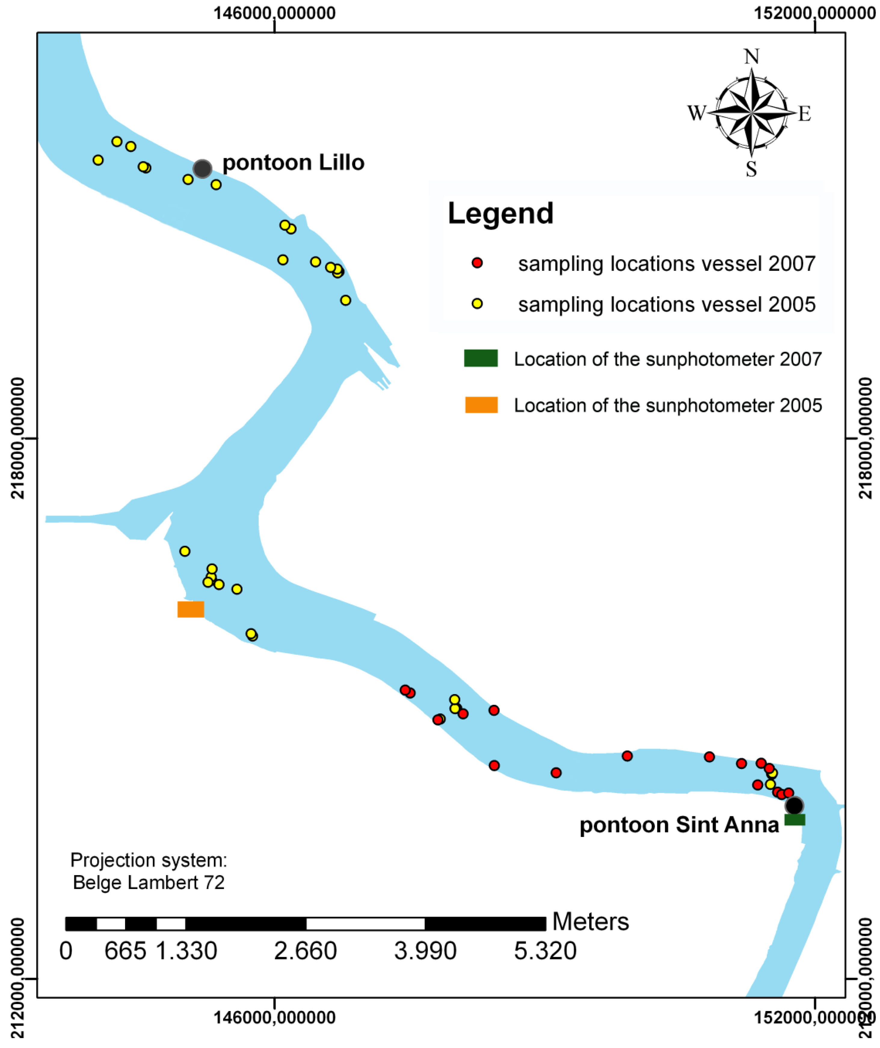
During the airborne campaigns in 2005 and 2007, the water-leaving reflectance was measured and surface water samples were gathered simultaneously with the overpass of the aircraft. The water was sampled using buckets in the upper 50 cm of the water column. The water samples were stored in dark bottles and were kept cool immediately after sampling. The sampling was done from vessels and from the fixed pontoons at Sint Anna and Lillo (
Figure 3). Several rules applied to the sampling from the vessels. First of all, the vessels need to lie idle during sampling to avoid turbulence effects. Secondly, the sampling positions need to be outside the main course of the ships; they have to include a large part of the study area and have a large variation in SPM concentration. Finally, sampling should be performed close to when the plane passes over. This last requirement is essential since the river is very dynamic and a match-up restriction of 5 min is applicable. The locations are indicated in
Figure 3. In total, 41 water match-up samples were gathered in 2005 and 17 water samples in 2007, which could be used to set up a robust SPM algorithm.
Figure 3.
Sampling locations.
Figure 3.
Sampling locations.
The water-leaving reflectance was measured on the vessels with an ASD (Analytical Spectral Devices, Inc.) FieldSpec FR spectrometer. The ASD spectrometer measures the reflected light in the Visible/Near Infrared (VNIR, 350–1,050 nm) and the Short-Wave Infrared (SWIR, 900–2,500 nm) portion of the spectrum. The downwelling irradiance above the surface (Ed(a)) was measured using an almost 100% reflecting Spectralon reference panel (Analytical Spectral Devices, Inc.). Then, the water-leaving radiance (Lw(a)) was measured by pointing the sensor at the water surface at 40° from nadir, maintaining an azimuth of 135° from the solar plane to minimize sun glint. Downwelling sky radiance (Lsky(a)) was measured at a zenith angle of 40° to account for the skylight reflection.
In addition to the field data obtained coincident with the airborne campaigns, extra samples were collected in June 2009 from vessels and monthly measurements were performed in 2007 at two pontoons at the Scheldt River near Antwerp (
Figure 3: pontoon Lillo and pontoon Sint Anna). These included water samples and measurements of the water-leaving reflectance and were done at the same time relative to High Water (HW),
i.e., at pontoon Sint Anna (SA) 2 h after HW and at pontoon Lillo (LI) 3 h after HW.
3.3 Lab Analysis of in situ Measurements
From the water samples, SPM concentration was determined by filtering the water on Whatman GF/F glass fiber filters according to the European reference method EN 872 [
21]. Following this method, the weight of the filters without particles is first measured and the filters are moistened with MilliQ-water. After shaking, 250 mL of the water samples are filtered. Then the filter is rinsed 3 times with 150 mL MilliQ-water to collect the residuals. The filter is dried in the oven for minimum 2 hours at 105 °C and is subsequently cooled in a desiccator for a minimum time of half an hour. Finally the filter is weighted and the concentration is derived.
SPM concentrations collected during the airborne campaigns in 2005 and 2007 ranged between 21 and 136.5 mg/L and between 17 and 115 mg/L respectively. In 2009 an average SPM concentration of 46 mg/L was found for the north part and 77.1 mg/L for the south part of the study area. In general, higher concentrations were observed for measurements closer to the shore and, in 2005, for measurements a few hours after high water.
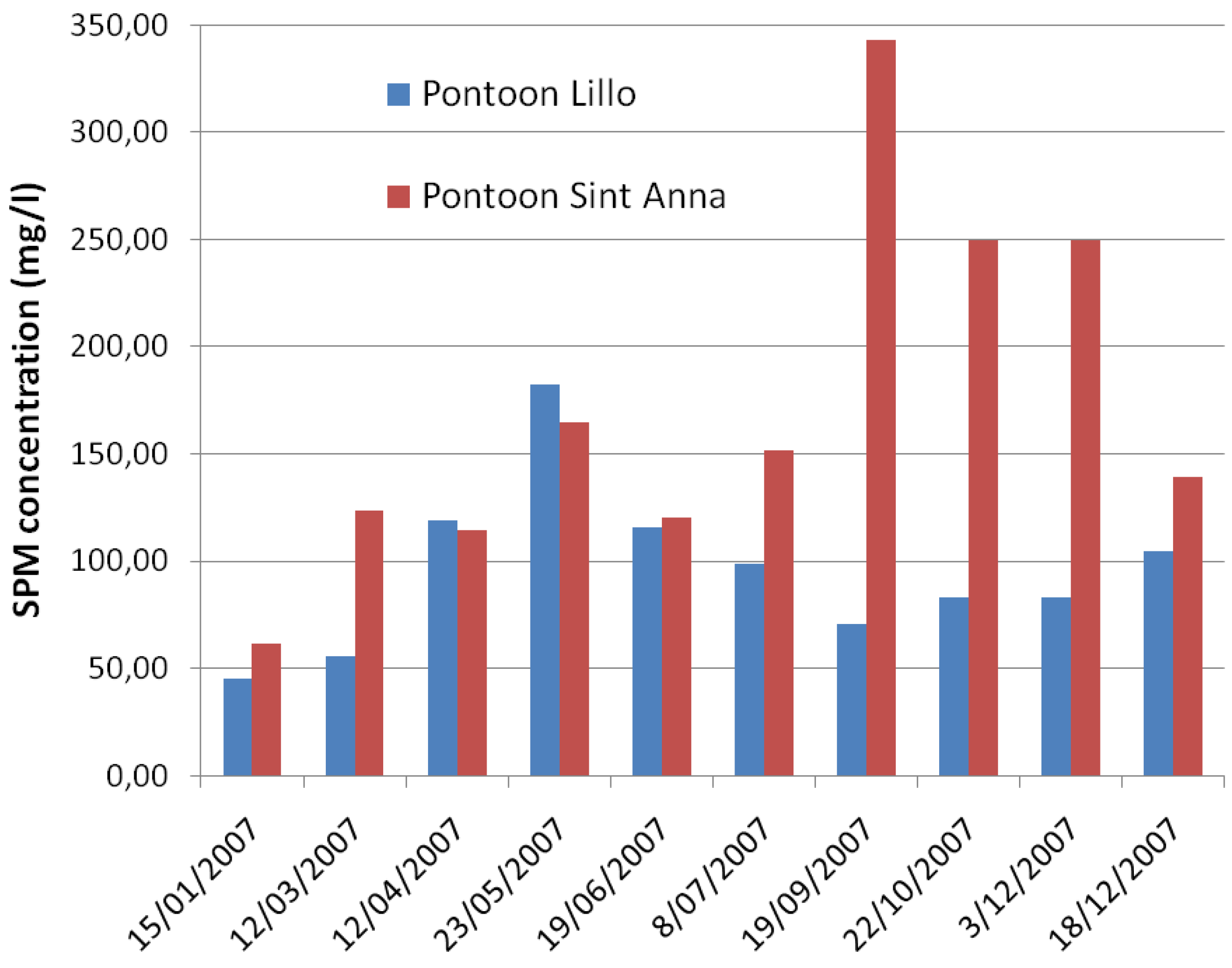
For the extra monthly
in situ sampling from the pontoons in 2007, the SPM concentration is shown in
Figure 4. The figure reveals strong seasonal variations with high differences between the two stations. For Lillo the highest SPM concentrations were recorded in May and the lowest in January. For Sint Anna, there is a local maximum in May and there is a remarkable strong increase in the autumn and beginning of the winter. These observations are difficult to interpret because of the lack of data. Moreover it is difficult to differentiate between local erosion/sedimentation and mud transport. In general, high concentrations appear more often in winter and low concentrations in summer [
18] due to variations in the freshwater discharge, temperature and land erosion. The higher values in May observed for both stations, could be due to a sudden increase in precipitation. April 2007 was an extraordinary month with no precipitation, whereas May was characterized by abnormal high precipitation [
22]. In autumn the precipitation was less than in the summer months, however the plant cover degrades nearing winter leading to higher terrestrial erosion. The lower concentrations in autumn and beginning of the winter for Lillo may indicate that Lillo is situated seaward of the turbidity maximum whereas Sint Anna could be located within this turbidity maximum.
Figure 4.
SPM averages for the extra monthly in situ measurements (2007).
Figure 4.
SPM averages for the extra monthly in situ measurements (2007).
The water-leaving reflectance (R
w) was calculated using the following equation [
23]:
where ρ
as is the air-sea interface reflection coefficient and is calculated as a function of the wind speed [
23]. Since the spectral resolution of the ASD (3 nm at around 700 nm) and AHS sensor are different, the
in situ measurements were resampled to match the response of the AHS sensor. The resampling was performed using a Gaussian model for each band by providing wavelengths and FWHM information of the AHS sensor
In
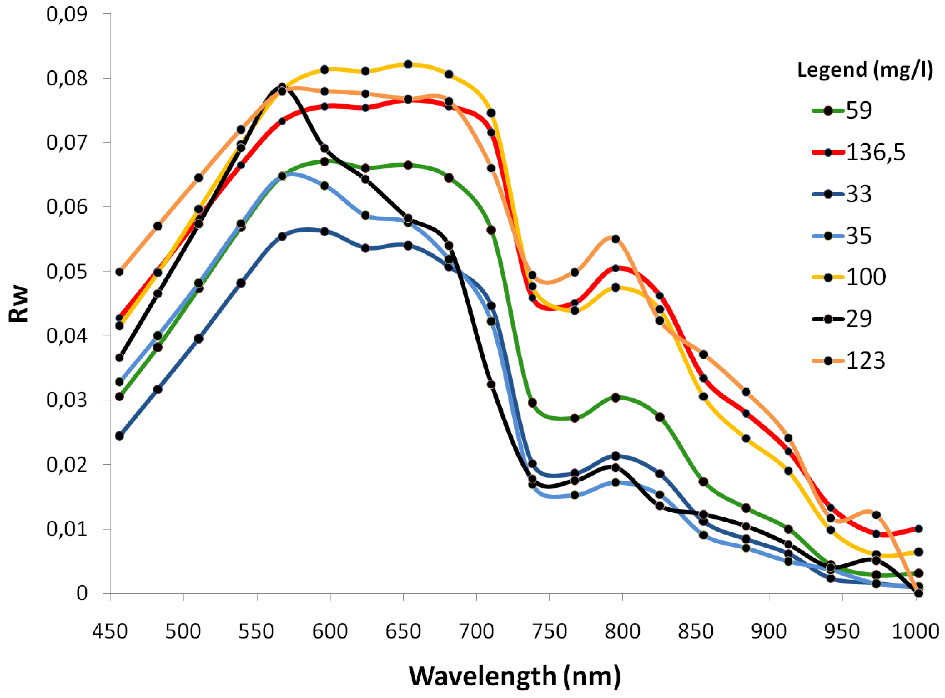
Figure 5, some of the measured water-leaving reflectance spectra are shown with their corresponding SPM concentration. For low SPM concentrations (<50 mg/L) a maximum is observed around band 5 (568 nm). The signal in the NIR is weak. At higher SPM concentrations this peak is no longer present and the signal between 568 nm and 681 nm is high and rather flat. For all spectra, a second but local maximum is observed in band 13 (795 nm). The reflectance spectra increases in the red and NIR with increasing SPM concentration. Largest increases are observed between 681 nm and 825 nm. Around 567 nm this steady increase is not apparent and, also at longer wavelengths (larger than 942 nm), the spectrum is less sensitive to increasing SPM concentrations.
The dataset collected covers much of the seasonal and tidal variations in the Scheldt River. Tidal influences are accounted for by the June 2005, October 2007 and June 2009 datasets. Seasonal variations are accounted for in the 2007 monthly dataset. The variations in SPM concentrations were shown and discussed in this section. Salinity or the composition of the sediment was not recorded. However, a big part of the variation is linked with variations in freshwater discharge and terrestrial erosion and, hence, with the precipitation. During periods of high river runoff, the salinity is low, whereas, during dry periods, high salinity values are observed [
18]. The tidal cycle (high salinity during high water, low salinity during low water) contributes to a lesser degree [
16]. Since the 2007 dataset covered a large range of precipitation values, it is assumed that it also covers a wide range in salinity values and it covers the existing changes in sediment composition.
Figure 5.
In situ measured water-leaving reflectance spectra.
Figure 5.
In situ measured water-leaving reflectance spectra.
4. Pre-Processing of the Airborne Images
Pre-processing of the airborne datasets was done in VITO’s Central Data Processing Centre (CDPC) for airborne data. The processing steps include archiving, dGPS correction, direct georeferencing, atmospheric, adjacency and air/water interface correction [
24]. The atmospheric and air-interface correction is based on the algorithms given in de Haan and Kokke [
25], which also takes into account the effects at the air/water interface:
The radiance received by the sensor
consists of atmospheric path radiance
, background path radiance
and ground reflected radiation
or
with
where
is the extraterrestrial solar irradiance,
is a coefficient describing the reflection of light by the atmosphere,
and
are respectively the sun zenith and azimuth angle,
and
are respectively the viewing zenith and azimuth angle,
is the downwelling irradiance above the surface,
tdif and
tdir are respectively the diffuse and direct ground-to-sensor transmittance,
Rapp is the target apparent reflectance defined as :
With the water-leaving radiance, the downwelling sky radiance. All these terms are measured just above the surface. is the Fresnel reflectance. is the background apparent reflectance, defined in a similar way as Rapp.
The water leaving reflectance
can be retrieved from
as follows:
The basis of the MODTRAN4 interrogation technique [
26,
25] is that apparent surface reflectance (
) and the water leaving reflectance
can be written as a function of
,
and several atmospheric parameters (
c1..5;
d1):
and
with
s* the spherical albedo of the atmosphere.
The
c1..5 and
parameters can be derived by running MODTRAN4. The visibility and water vapor content were estimated from the images according to the methods described in [
27] and [
28]. The aerosol type was derived from the spectral dependency of the aerosol optical depths obtained from ground-based sunphotometer readings as the airplane passed over (
Figure 2) [
29].
An adjacency correction was performed based on the NIR similarity spectrum [
30]. This correction algorithm estimates the contribution of the background radiance based on the correspondence with the NIR similarity spectrum. The main advantage of the method is that no assumptions have to be made on the NIR albedo, such that the correction can be applied over more turbid waters,
i.e. until the similarity spectrum is valid (0.3 to 200 mg/L according to [
31,
32]).
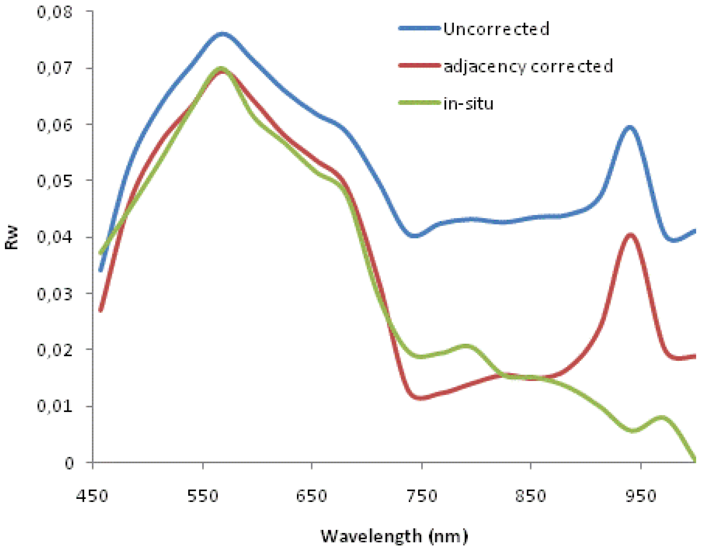
Figure 6 shows a water-leaving reflectance spectrum before and after adjacency correction and a coincident
in situ measurement. Without adjacency correction, the water-leaving reflectance is high in the NIR due to the presence of vegetation near the shores. After the correction, the NIR reflectance decreased significantly and matched the
in situ spectrum better. Small deviations between the
in situ and airborne spectrum can be due to match-up problems during sampling. The water vapor absorption band is still apparent in the airborne spectra. However during operational processing this absorption feature will no longer be visible as the water vapor is automatically estimated from the image according to [
28].
Figure 6.
Water-leaving reflectance spectra from an airborne image before and after adjacency correction compared with an in situ above water measurement of the water‑leaving reflectance.
Figure 6.
Water-leaving reflectance spectra from an airborne image before and after adjacency correction compared with an in situ above water measurement of the water‑leaving reflectance.
6. Results and Discussion
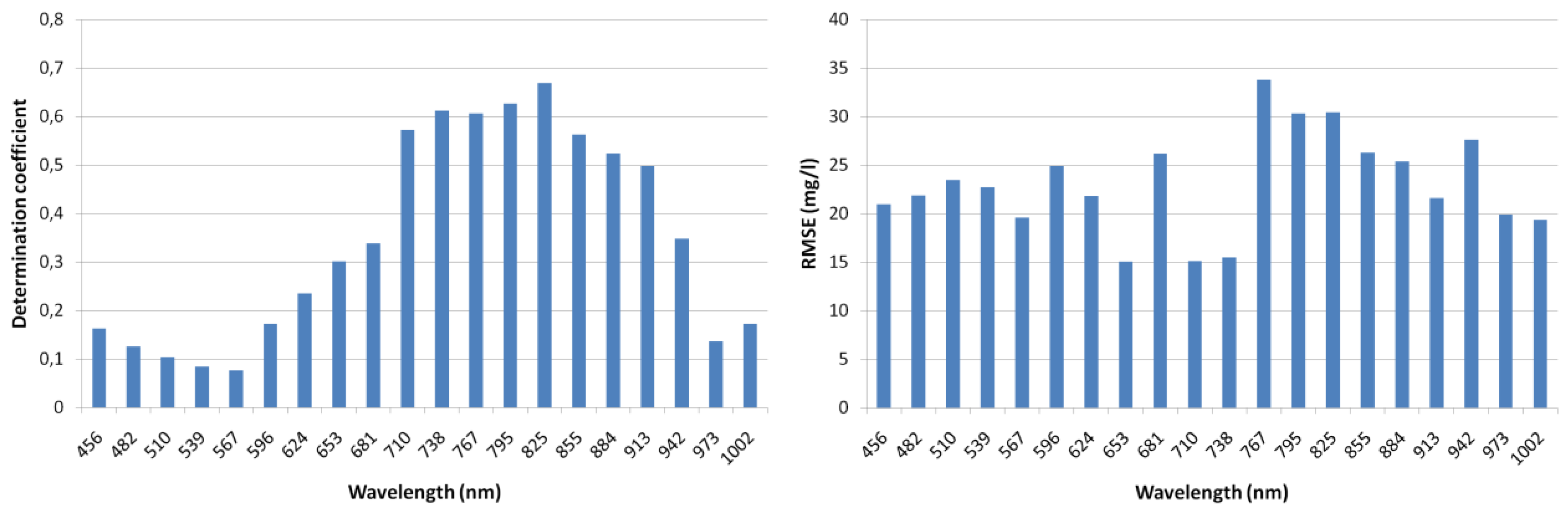
Figure 7 shows the results for single band relationships and
Table 3 shows the best performing regression models for multi-band relationships with their corresponding correlation coefficient, determination coefficient, RMSE, slope and intercept. From
Figure 7, it is clear that the Red and NIR wavelength range from 710 nm to 913 nm is highly sensitive to increases in SPM concentration. From visual inspection of the water-leaving reflectance spectra (
Figure 5), similar conclusions were drawn. The highest single-band correlation (determination coefficient of 0.67) is obtained for the 825 nm band. The RMSE is 30.45 mg/L. Furthermore, bands 710 and 738 are interesting because of their low RMSE (15.08 mg/L and 15.51 mg/L respectively). For the multi-band relationships, only band ratios and band differences are shown with exponential relationships because these outperformed all the others. Most of the algorithms in
Table 3 combine a high correlation band with a low correlation band, resulting in even higher correlations. By combining these bands errors in the correction for surface reflection effects (sun and sky glint), the water-leaving reflectance spectra might by cancelled out. The problem in the correction of these surface reflection effects, lies in the ρ
as factor which is the air‑sea interface reflection coefficient and is calculated as a function of the wind speed. This factor is an approximation and probably contains some errors which can be minimized by considering band ratios or band differences.
The highest determination coefficient (0.81) and lowest RMSE (15.07 mg/L) was obtained for a model using a visible to red band ratio (Rw539/Rw795).
Figure 7.
Determination coefficient and RMSE for single band relationships.
Figure 7.
Determination coefficient and RMSE for single band relationships.
All relationships in
Table 3 were validated using water-leaving reflectance spectra from the airborne AHS datasets. In general, a higher RMSE is observed compared to the results of the
in situ measurements. This can partly be attributed to inaccuracies in the atmospheric correction. Only the best performing band ratios and band difference are presented in
Table 4. The band ratios perform much better than the band differences. In particular two band ratio algorithms have very good validation results:
Table 3.
Results of the regression analysis for multi-band relationships.
Table 3.
Results of the regression analysis for multi-band relationships.
| Algorithm | Slope | Intercept | Correlation Coefficient | Determination Coefficient | RMSE (mg/L) |
|---|
| 596/653 | −8,21 | 12,60 | −0,78 | 0,60 | 20,95 |
| 596/681 | −5,11 | 9,66 | −0,74 | 0,55 | 21,86 |
| 456–710 | −39,26 | 3,30 | −0,74 | 0,54 | 23,49 |
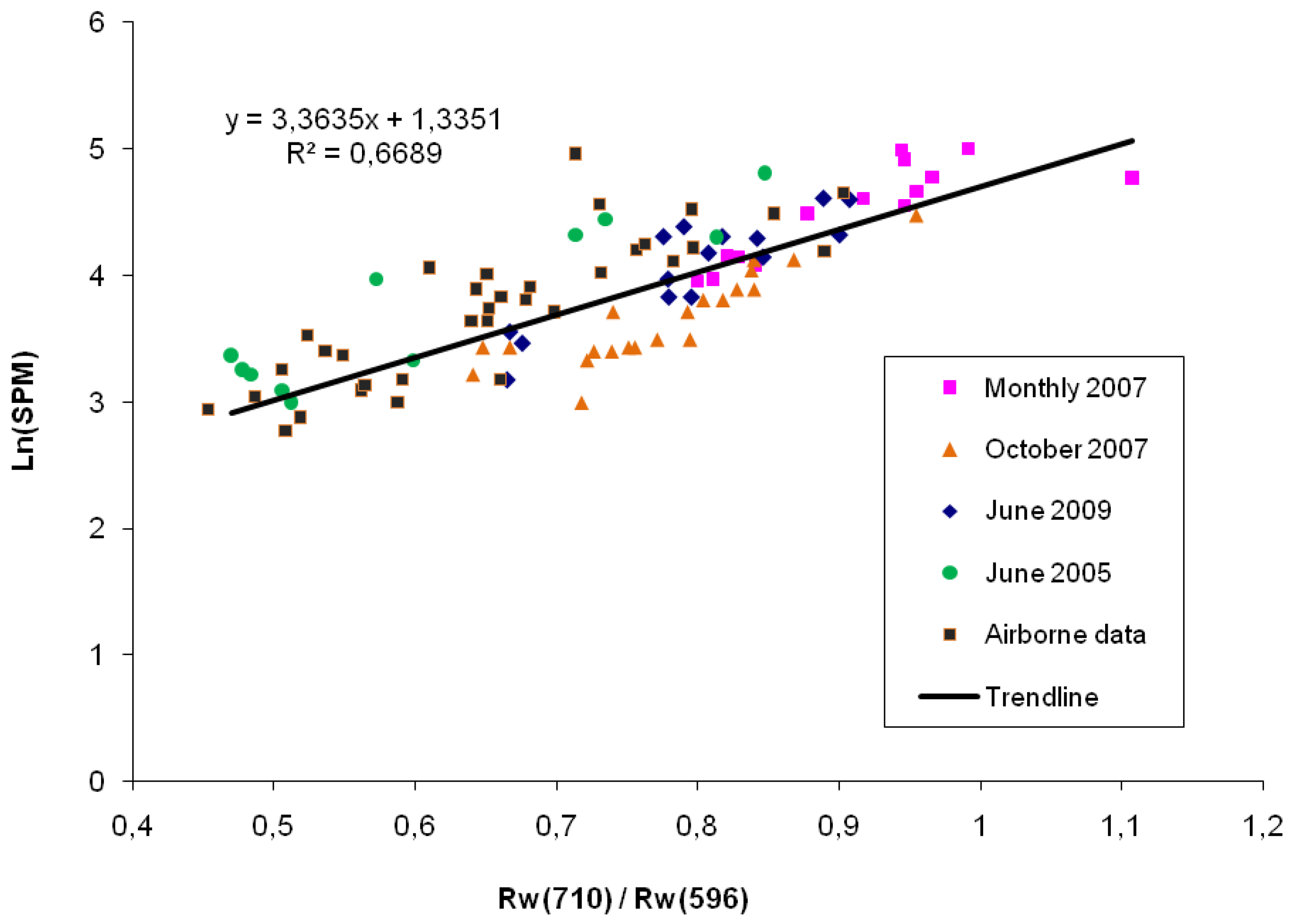
| 710/596 | 3,36 | 1,34 | 0,82 | 0,67 | 19,58 |
| 710/539 | 2,37 | 1,86 | 0,78 | 0,61 | 21,81 |
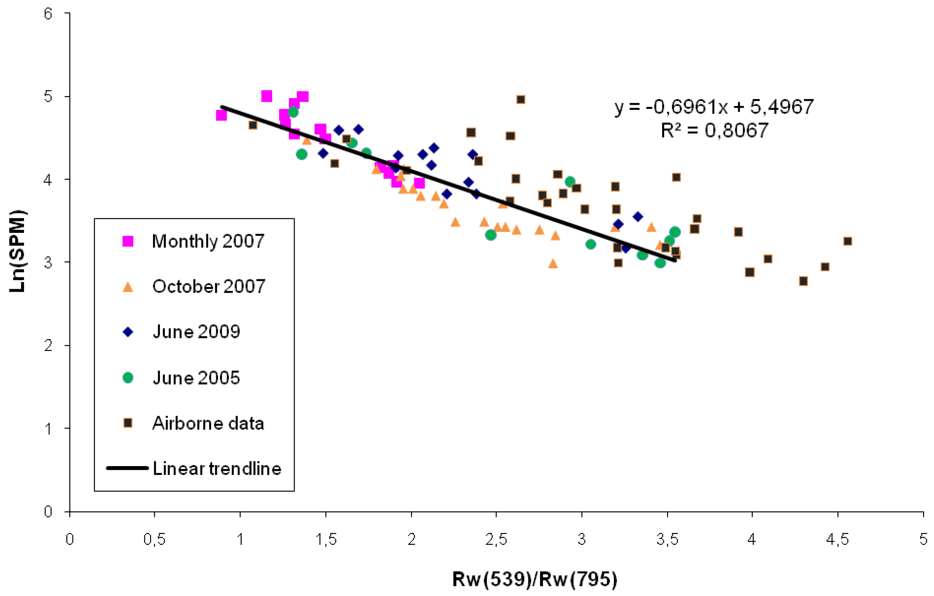
| 539/795 | −0,70 | 5,50 | −0,90 | 0,81 | 15,07 |
| 510/795 | −0,85 | 5,54 | −0,90 | 0,80 | 15,09 |
| 1002–767 | −38,39 | 3,07 | −0,75 | 0,56 | 26,31 |
| 1002–795 | −36,00 | 3,01 | −0,77 | 0,59 | 25,38 |
| 1002–825 | −43,46 | 2,98 | −0,83 | 0,68 | 21,60 |
| 973–767 | −48,20 | 2,90 | −0,84 | 0,71 | 19,88 |
| 973–795 | −43,72 | 2,86 | −0,85 | 0,72 | 19,35 |
| 973–825 | −46,06 | 2,98 | −0,85 | 0,72 | 20,32 |
| 973–855 | −62,95 | 3,10 | −0,83 | 0,69 | 21,15 |
| 942–767 | −51,46 | 2,91 | −0,82 | 0,67 | 22,72 |
| 942–795 | −46,46 | 2,86 | −0,83 | 0,68 | 21,82 |
| 942–825 | −53,75 | 2,90 | −0,86 | 0,75 | 18,96 |
| 942–855 | -68,90 | 3,13 | −0,80 | 0,63 | 23,67 |
| 942–884 | −85,90 | 3,22 | −0,77 | 0,59 | 25,73 |
| 913–825 | −75,92 | 2,85 | −0,85 | 0,71 | 20,48 |
| 913–855 | −138,82 | 3,00 | −0,81 | 0,65 | 22,37 |
| 913–884 | −235,70 | 3,14 | −0,75 | 0,56 | 26,26 |
| 913–973 | 106,14 | 3,24 | 0,82 | 0,66 | 23,33 |
| 539–681 | −67,95 | 3,91 | −0,75 | 0,57 | 22,14 |
Table 4.
Results of validation with the airborne data.
Table 4.
Results of validation with the airborne data.
| Band Combination Algorithm | RMSE (mg/L) | RMSE (%) |
|---|
| 710/596 | 16,10 | 29,02 |
| 539/795 | 18,36 | 35,29 |
| 1002–767 | 34,85 | 54,96 |
| 1002–795 | 33,34 | 50,99 |
| 1002–825 | 32,88 | 50,35 |
| 973–825 | 34,75 | 54,66 |
These band ratio algorithms are not in line with previous findings for the Scheldt River. In [
15] a band difference algorithm of two NIR bands was obtained after a similar regression analysis. The regression analysis was based solely on the airborne dataset with 15 flight lines all acquired on 15 June 2005 (same dataset as used in this study). The RMSE obtained for this band difference was 15 mg/L. However, the airborne dataset used was not corrected for adjacency effects. The band difference worked very well in this particular case as it seemed to partly correct these adjacency effects. Here, using an extended seasonal dataset which is corrected for adjacency effects, similar band ratio algorithms result in a RMSE of around 33 mg/L. These results were expected due to the large tidal, seasonal and yearly variations in the dataset.
In contrast, band ratio algorithms (10) and (11) provide surprisingly good results. Looking beyond the Scheldt River, comparable band ratio algorithms were found for the Bristol channel (618 nm/754 nm) and the Norfolk coast (575 nm/747 nm) by Matthews
et al. [
11] using a CASI hyperspectral sensor. Doxoran
et al. [
12,
13] established a robust relationship between SPM and a near-infrared to red band ratio (850 nm/550 nm) for the Gironde and Loire estuary based on
in situ spectral measurements. Both authors point to the seasonal robustness of their algorithms, but both their algorithms needed recalibration when applying them to different estuarine environments [
13]. Hence the frequent use of these band ratios and the SPM concentrations indicates the robustness of these algorithms however they seem to be site specific. The characteristics of the suspended sediment (particle size and type) strongly vary between the different sites (much more than the seasonal variability). Especially for estuaries these variations can be large as they depend on the upland basins, river discharge, tidal cycles and flocculation processes. These characteristics influence the scattering behavior and, consequently, these empirical algorithms are no longer valid when applied to these other environments.
The two band ratio algorithms (10) and (11) retrieved after the regression analysis and the validation with the airborne data are presented graphically in
Figure 8 and
Figure 9. All
in situ datasets used to build the algorithm are shown in different colors. The trend line in black shows the relationships as obtained after the regression analysis. The airborne dataset is superimposed on this graph. These figures show the robustness of the algorithms as all datasets are quite well distributed among the trend line. All datasets have a minor offset from the trend line and in particular two datasets have a slightly different slope: the monthly dataset for SPM algorithm 11 and the June 2009 dataset for SPM algorithm 10. It is therefore recognized that an algorithm specifically calibrated for each dataset will have a better correlation and better SPM estimates but, from the point of view of a robust algorithm, these two algorithms perform surprisingly well. Since algorithm (10) performs better for the airborne data, this algorithm is selected as seasonally robust algorithm for the Scheldt.
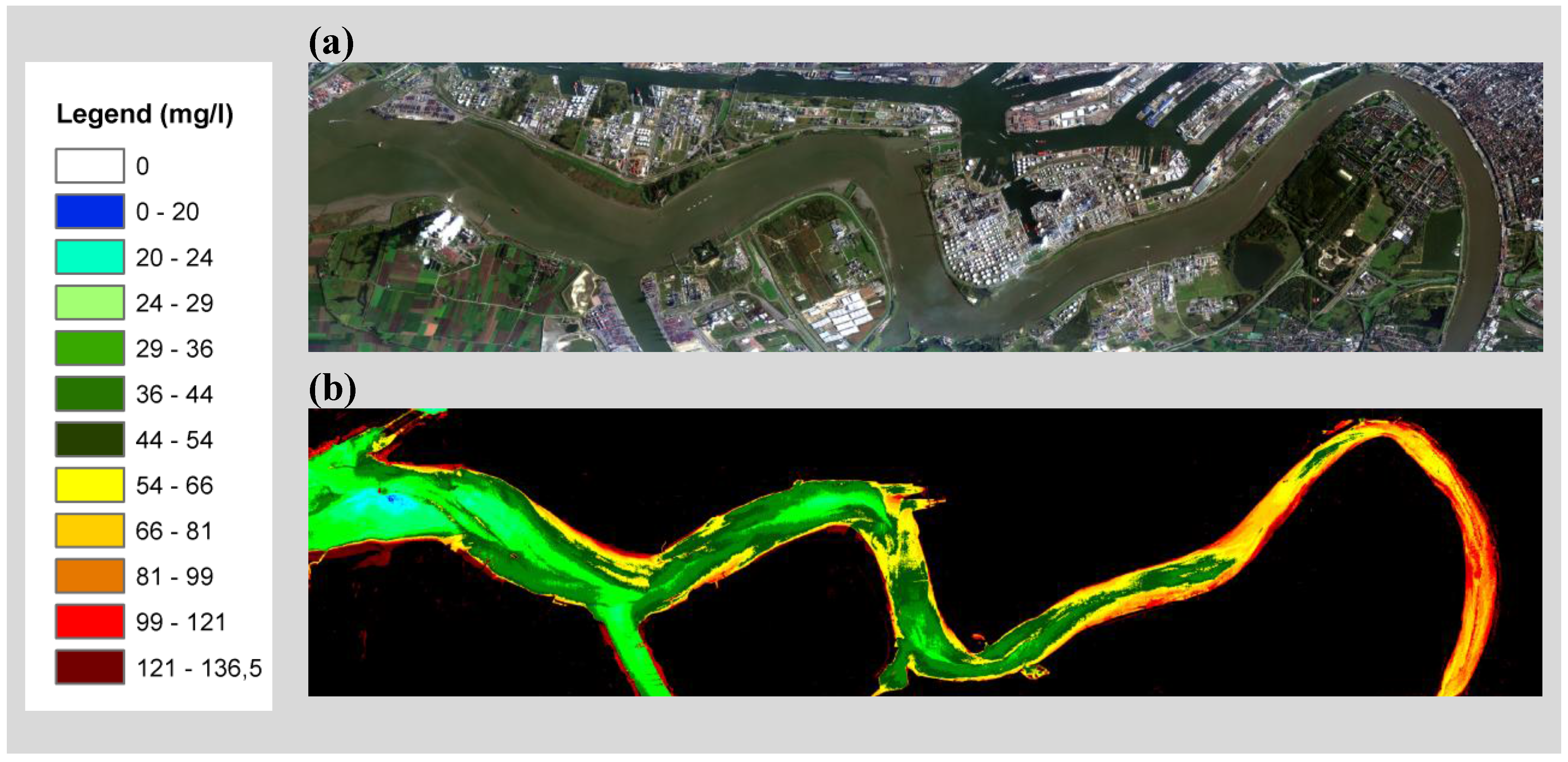
Finally algorithm (10) which provided the best validation results was applied to the airborne dataset to derive an SPM concentration map. Since the SPM concentration values were log transformed, an additional correction for statistical bias is needed when performing the back-transformation [
33]:
with s
2 as the variance.
The final SPM concentration map is shown in
Figure 10. The concentrations are expressed in mg/L and an exponential color bar was chosen to best represent the data. The concentrations were in the expected range. No adjacency effects are observed. Increasing concentrations on the sides are interpreted as natural increases of the surface SPM concentration and are not linked to adjacency.
Figure 8.
SPM Algorithm 10.
Figure 8.
SPM Algorithm 10.
Figure 9.
SPM Algorithm 11.
Figure 9.
SPM Algorithm 11.
Figure 10.
(a) Hyperspectral image of the Scheldt river, 6 June 2009, 10:03 UTC, (b) SPM concentration map of the Scheldt River.
Figure 10.
(a) Hyperspectral image of the Scheldt river, 6 June 2009, 10:03 UTC, (b) SPM concentration map of the Scheldt River.
7. Conclusion
An extensive dataset was gathered in this study to find a seasonally robust algorithm for SPM estimation in the Scheldt River near Antwerp. The
in situ measurements were used to set up the algorithm and two airborne hyperspectral datasets were used for validation. The selected seasonally robust algorithm uses a ratio of a band at 710 nm and a band at 596 nm. This ratio is exponentially related to the SPM concentration. The use of similar band ratios found in the literature indicates the robustness of these algorithms. The advantage of this robust algorithm is mainly its wide applicability without any
in situ sampling and the associated reduction in cost. On the contrary, algorithms specifically calibrated for one moment and one area are more expensive but are proven to provide higher accuracies [
15]. With an eye on temporal follow up of the SPM concentrations in the Scheldt estuary, the seasonal robustness may be more important than the absolute accuracy of the algorithm, and the band ratio algorithm found in this study may be ideal. Also when only a few (or no)
in situ measurements are available, this algorithm could provide an idea of the concentrations and patterns in the Scheldt River. If highly accurate SPM estimates are needed for one specific moment in time, it could still be worthwhile to recalibrate the algorithm using
in situ measurements.
In the coming years new datasets will be acquired over the Scheldt area, also with new hyperspectral sensors like APEX (Airborne Prism Experiment). These datasets will be used to further validate and, if needed, to improve the current band ratio algorithm.
In general, this paper has clearly indicated the potentials of remote sensing for assessing the surface water quality of rivers and estuaries. Nevertheless remote sensing data are rarely used in river/estuarine management practices. The advantages are however manifold and the surplus value to conventional in situ sampling is evident: a high spatial variability, a synoptic view, high repeatability. The restricted use of these data might on one hand be due to the spectral and spatial limitations of current satellite sensors and, on the other hand, the high cost involved in airborne acquisitions. In fact, for these estuarine studies, data/sensor requirements include frequent revisits that increase image collection opportunities, high spatial (~10 m) and high spectral resolution or tunable spectral bands. Nowadays no single sensor on a satellite platform combines these specifications. Future missions look likely to follow the trend towards higher spatial and spectral resolutions but the temporal requirement will not be fulfilled in the near future. Imagery is often only acquired on demand, restricted by on-board storage capacity. In the near future an airborne system is therefore the only feasible solution for the problem at hand. In this study, the flexibility of the airplane has proven to be a big advantage because of (1) the difficulty to obtain cloud-free data in this area and (2) having the possibility to fly several tracks in a row, thereby increasing the number of coincident in situ samples. In order to reduce the cost associated with these airborne campaigns, and increase the flexibility even more, new Unmanned Aerial Systems (UAS) seem to be the way to go. Especially with growing interest in the development of light weight sensors that can be mounted on these UAS, for multispectral as as well hyperspectral, these systems provide a cost efficient and highly flexible alternative for the airborne acquisitions.
Besides these technological developments, there is a strong need to focus on atmospheric corrections, including the correction for adjacency effects, and to improve the calibration of spaceborne and airborne sensors.


