1. Introduction
Biophysical parameters including landcover [
1], land surface temperature (LST) [
2], tree canopy density [
3],
etc., are of great importance in assessing environmental change. Modern operational space-borne sensors with spectral sensitivity in the thermal infra-red spectrum allow monitoring of the Earth’s thermal field at a moderate spatial resolution [
4]. Thermal imagery products are available on a regular and frequent basis for both land and oceans [
2,
5].
Accordingly, digital elevation models (DEMs) are freely available through the Internet [
6], providing global coverage and assisting various environmental applications. Various quantitative techniques (terrain modeling) have been developed to automate the extraction of terrain features from DEMs [
7]. Terrain modeling includes terrain segmentation into elementary objects, parametric representation and classification of objects, on the basis of their spatial three-dimensional arrangement [
8]. These methods allow recognizing and monitoring of natural hazards and environmental change [
9,
10].
Egypt includes many regions of diverse environmental characteristics, landcover and biophysical conditions [
11]. The quantification of the knowledge related to the various regions of Egypt is a key factor in the attempt to characterize the landscape, assess the sensitivity against natural hazards and support environmental analysis and planning at moderate resolution scale.
The goal of this research was to integrate monthly MODIS Land Surface Temperature data with elevation data to map climatic zones of Egypt. Such effort could assist environmental assessment and urban planning at a country level.
2. Methodology
Initially, the digital elevation data and the LST multi-temporal imagery of the study area are presented. The terrain was segmented through k-means clustering into regions, representing a distinct annual thermal signature. Finally, each region was parametrically represented on the basis of both its thermal signature and elevation statistics.
2.1. DEM of the Study Area
The study area corresponds to Egypt, bounded by latitudes 21.75° to 31.65° North and longitudes 24.72° to 35.77° East. The Shuttle Radar Topography Mission (SRTM) successfully collected Interferometric Synthetic Aperture Radar data over 80% of the landmass of the Earth between 60° North and 56° South latitudes on February 2000 [
12]. In its original release, SRTM data contained regions of no-data (named voids), specifically over water bodies (lakes and rivers), and in areas where insufficient textural detail was available in the original radar images to produce three-dimensional elevation data. The existence of voids causes significant problems in using SRTM DEMs [
6]. The Consortium for Spatial Information of the Consultative Group for International Agricultural Research is offering post-processed void-free 3-arc second SRTM DEM data for the globe [
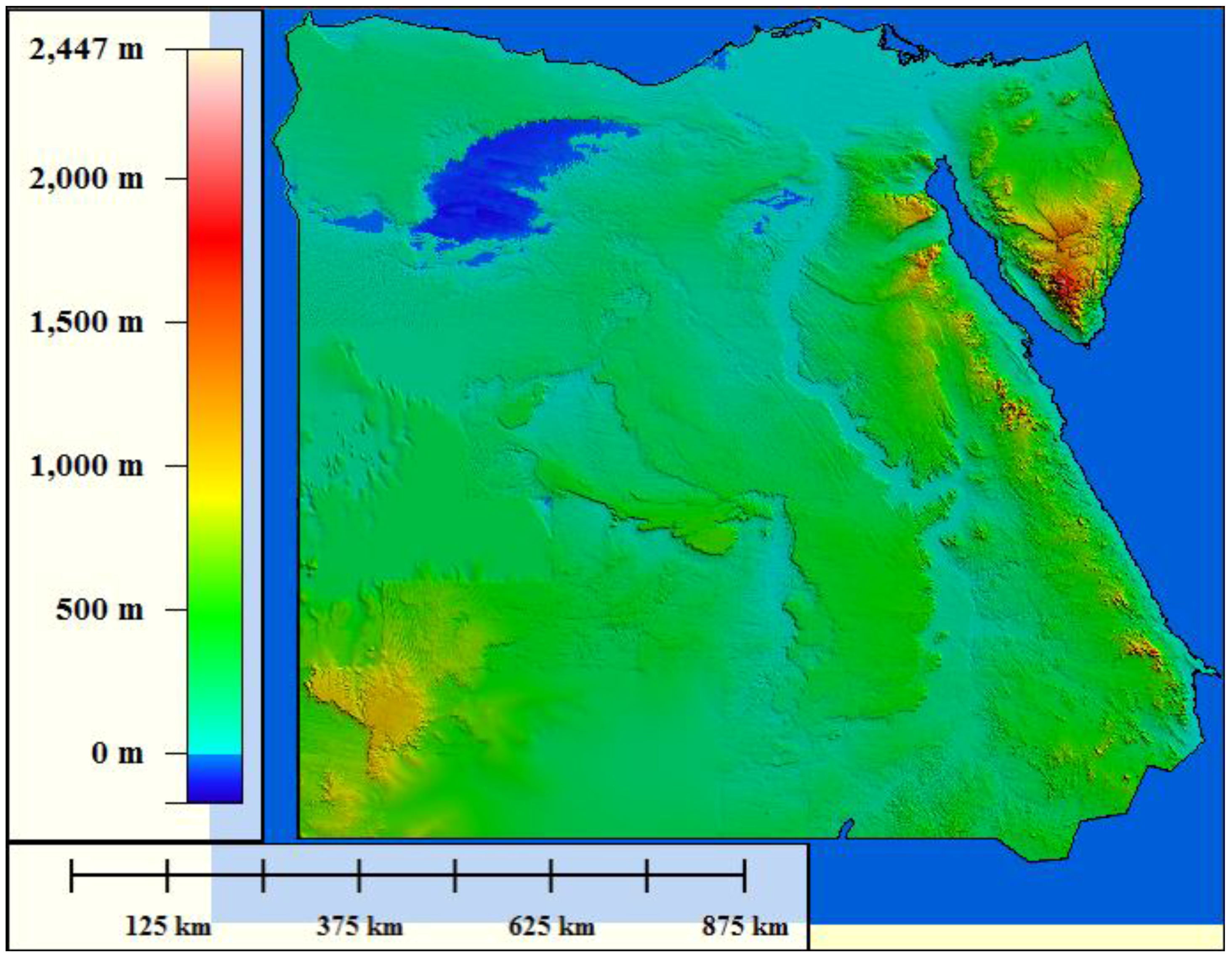
13]. The DEM data is available in 5° tiles, referenced to WGS-84 ellipsoid, forming a geographic grid with spacing 3 arc seconds. The SRTM DEM of the study area is presented in
Figure 1.
Figure 1.
The Shuttle Radar Topography Mission (SRTM) digital elevation model DEM of the study area, forming a geographic grid referenced to WGS-84 ellipsoid with spacing 3 arc seconds. The elevation range is within the interval [−170, 2,447] m. The Nile River crossing the east portion of Egypt from north to south is easily recognized as the elongated, smooth, low relief region in respect to the surrounding land.
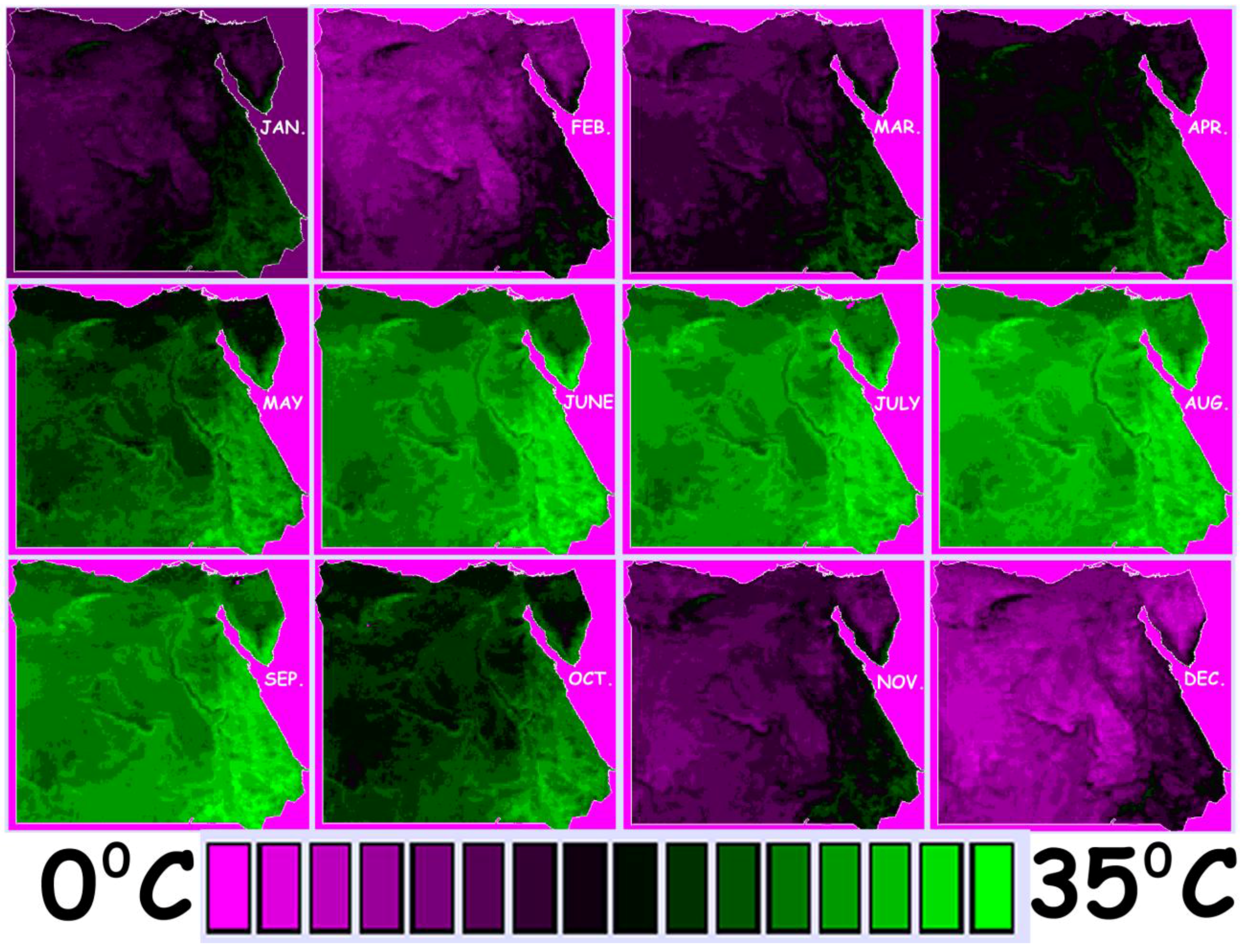
2.2. Multi-Temporal LST Data of the Study Area
The LST algorithm used to obtain MYD11C3 uses as input data including geolocation, radiance, cloud masking, atmospheric temperature, water vapor, snow, and land cover. Validated LST values within a calendar month are composited and averaged. MYD11C3 provides validated day/night LST values on a 0.05 degree latitude/longitude grid (5,600-meter at the equator) Thus, accuracy has been assessed over a widely distributed set of locations and time periods via several ground-truth and validation efforts. These data are ready for use in scientific publications when monthly averaged LSTs are application-appropriate [
14].
The 12 images that correspond to the monthly averaged night (10:30 PM pass) LST of the year 2006 are shown in
Figure 2.
Figure 2.
Monthly night land surface temperature (LST) values (the darker a pixel is, the greater the LST). From March to October the Nile River is easily identified due to the observed lower LST values compared to the surrounding land.
Figure 2.
Monthly night land surface temperature (LST) values (the darker a pixel is, the greater the LST). From March to October the Nile River is easily identified due to the observed lower LST values compared to the surrounding land.
2.3. Thermal Terrain Segmentation
K-Means cluster analysis was used to partition the 12-dimensional imagery into K exclusive clusters. In general, k-means initiate by positioning cluster centroids, then assigns each pixel to the cluster whose centroid is nearest, updates the centroids, then repeats the process until the stopping criteria are satisfied [
15]. It uses Euclidian distance to calculate the distances between pixels and cluster centroids.
The 12 thermal images (
Figure 2) represented a common arithmetic range of values in the interval [−2, 35] degrees Celsius and there was no need for data standardization. In the current implementation of the method, small clusters with area extent (occurrence) less than 0.5% were eliminated by merging them with larger clusters that are closest to their centroids. The stopping criterion was defined as a threshold in the percentage of the migrating pixels during a specific iteration (if it was less than 0.1% of the entire image pixels, clustering was terminated). Eight clusters were mapped after 73 iterations. The cluster centroids are given in
Table 1.
Table 1.
LST cluster centroids, as well as occurrence (percent area extent) and mean/standard deviation (S.D.) of elevation per cluster. The clusters are presented in decreasing mean LST order (7, 1, 8, 6, 3, 5, 4, 2) for the months May to September.
Table 1.
LST cluster centroids, as well as occurrence (percent area extent) and mean/standard deviation (S.D.) of elevation per cluster. The clusters are presented in decreasing mean LST order (7, 1, 8, 6, 3, 5, 4, 2) for the months May to September.
| Parameter | Month | Clusters
(in decreasing mean LST order from May to September) |
|---|
| 7 | 1 | 8 | 6 | 3 | 5 | 4 | 2 |
|---|
LST
Centroids
(°C)
| January | 15.7 | 12.2 | 8.9 | 5.9 | 3.7 | 6.8 | 4.0 | 6.5 |
| February | 17.0 | 13.7 | 11.1 | 8.5 | 6.4 | 9.4 | 6.6 | 7.8 |
| March | 20.5 | 17.6 | 15.1 | 13.6 | 12.0 | 12.8 | 10.5 | 10.3 |
| April | 22.9 | 20.4 | 17.9 | 16.9 | 15.7 | 16.0 | 14.3 | 14.2 |
| May | 27.6 | 25.5 | 23.2 | 21.9 | 20.7 | 20.5 | 18.6 | 17.6 |
| June | 31.0 | 29.3 | 26.6 | 25.9 | 24.8 | 24.2 | 22.5 | 22.0 |
| July | 30.8 | 29.4 | 27.2 | 26.8 | 25.7 | 25.3 | 23.9 | 23.3 |
| August | 31.0 | 30.0 | 28.4 | 28.3 | 27.5 | 26.6 | 25.2 | 24.4 |
| September | 30.6 | 28.5 | 26.0 | 25.1 | 24.1 | 24.0 | 22.4 | 22.0 |
| October | 26.6 | 23.8 | 21.3 | 19.9 | 18.6 | 19.2 | 17.5 | 18.3 |
| November | 18.8 | 15.9 | 12.8 | 11.9 | 10.7 | 11.4 | 9.7 | 12.0 |
| December | 15.0 | 11.7 | 8.4 | 6.9 | 5.1 | 7.1 | 4.6 | 8.5 |
| Occurrence (%) | 9.0 | 11.2 | 17.2 | 14.2 | 21.4 | 9.6 | 10.0 | 7.4 |
| Elevation (m) | Mean | 336 | 320 | 316 | 237 | 236 | 388 | 427 | 107 |
| S.D. | 166 | 217 | 227 | 168 | 107 | 295 | 284 | 127 |
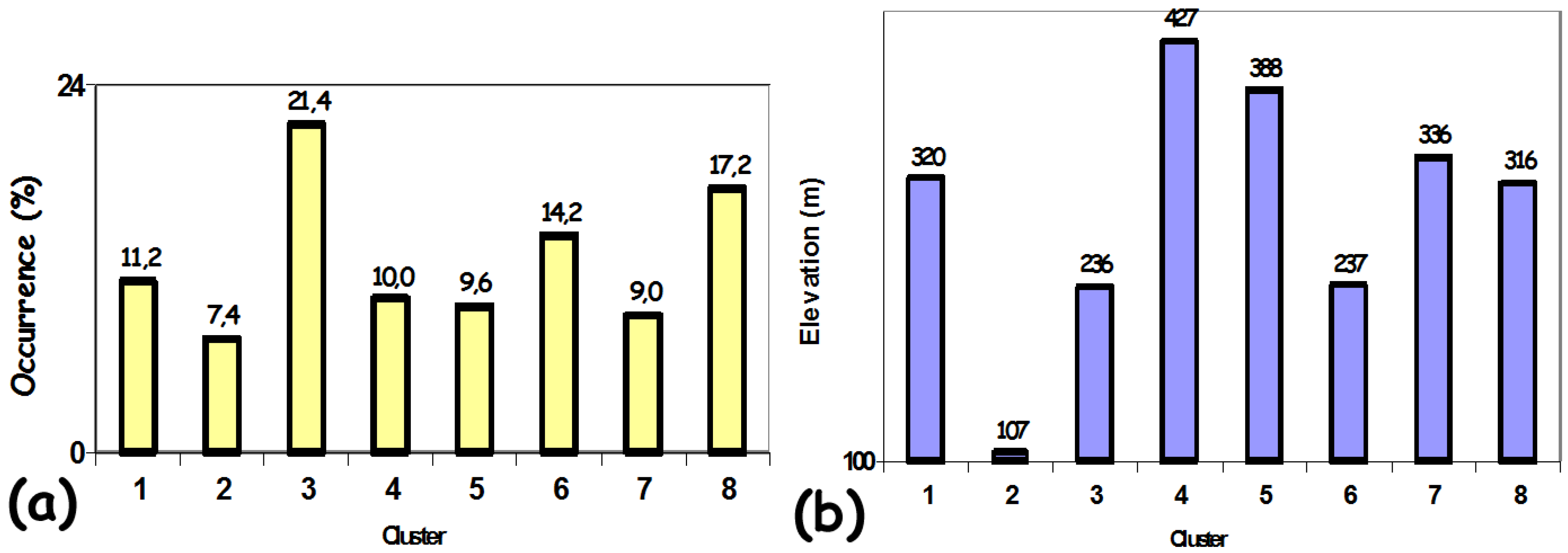
The cluster occurrence (percent area extent per cluster), as well as elevation statistics (mean elevation and standard deviation of elevation) per cluster are shown in
Table 1. The cluster occurrence and elevation statistics are graphically presented in
Figure 3.
Figure 3.
(a) Percent area of each cluster class. (b) Mean elevation within each cluster class.
Figure 3.
(a) Percent area of each cluster class. (b) Mean elevation within each cluster class.
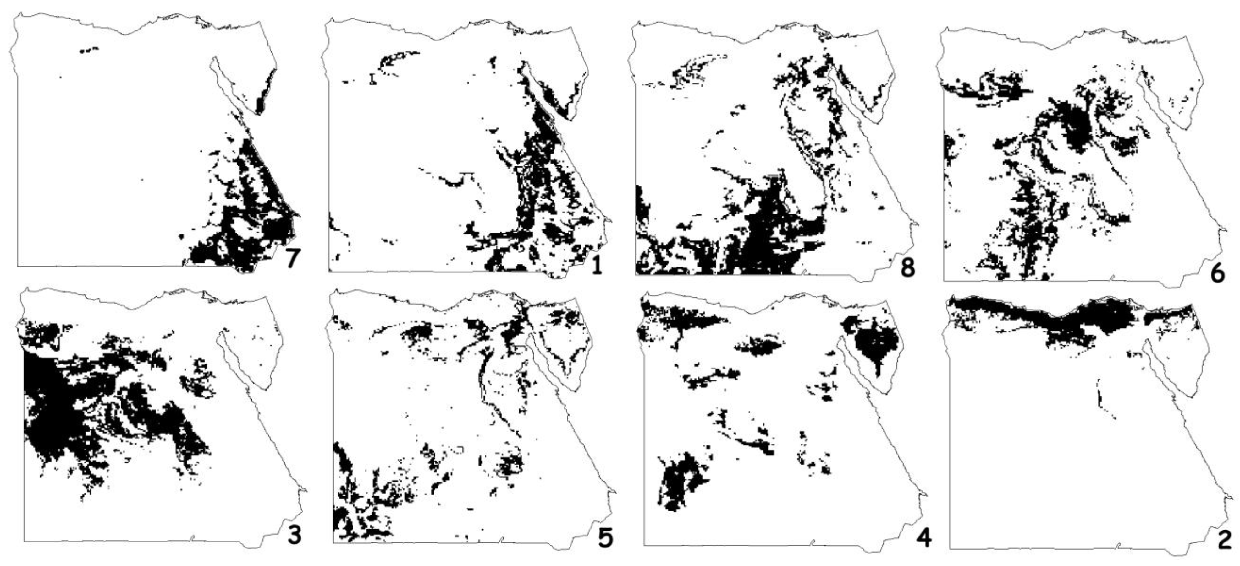
The spatial distribution of the eight clusters is shown in
Figure 4, while the temporal distribution of the cluster centroids’ LST is presented in
Figure 5.
Figure 4.
Spatial distribution of the eight cluster centroids.
Figure 4.
Spatial distribution of the eight cluster centroids.
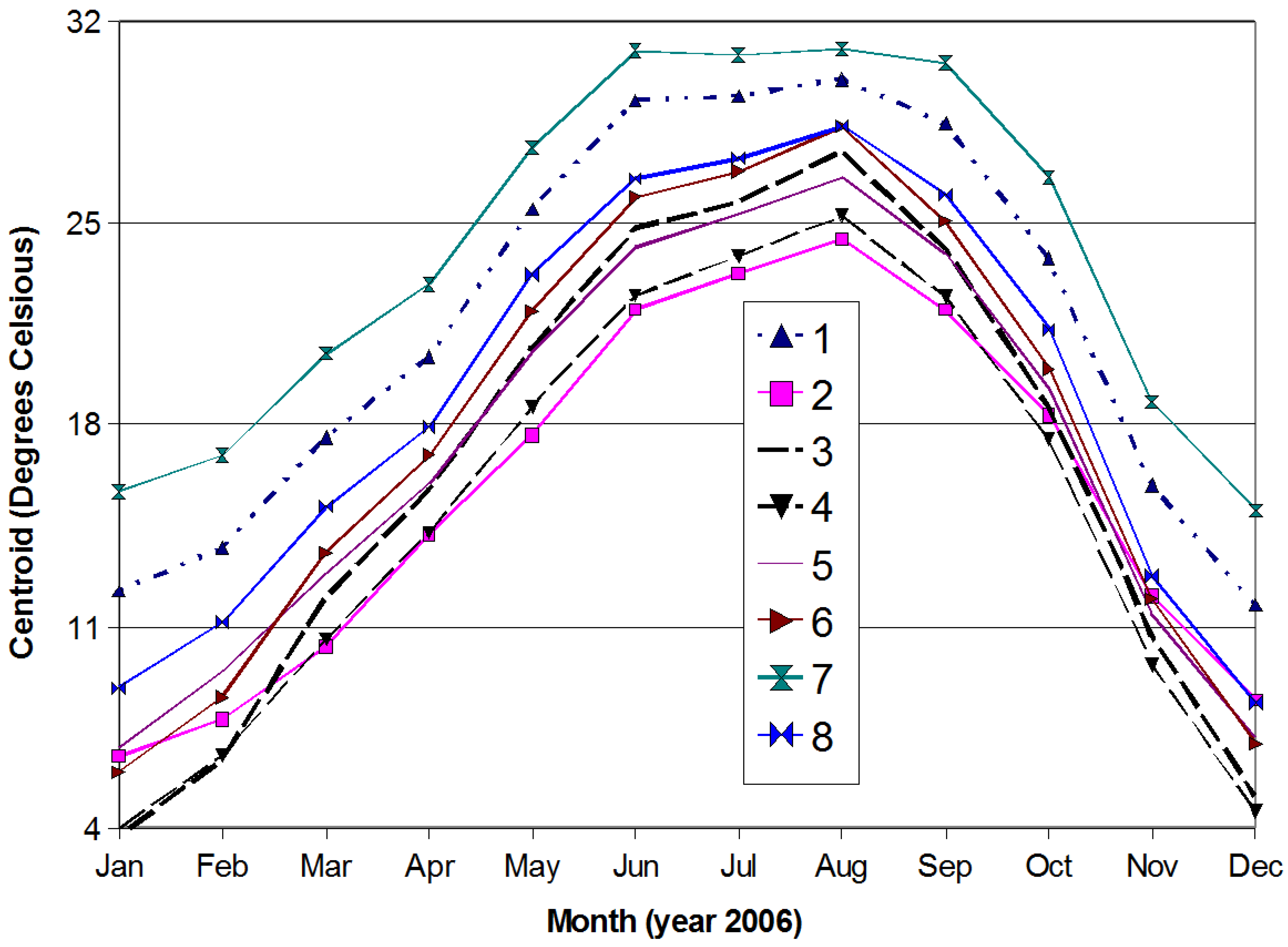
Figure 5.
Temporal distribution of the eight cluster centroids.
Figure 5.
Temporal distribution of the eight cluster centroids.
2.4. Spatially Fused Clustering
A variation of the multi-temporal image sequence clustering was also performed in order to explicitly incorporate spatial proximity, not addressed in the previously discussed process. Thus, the LST image dataset was supplemented with two additional parameters, corresponding to the spatial (x, y) coordinates. These additional images were defined in an arbitrary pixel coordinate system, scaled in accordance to the LST data.
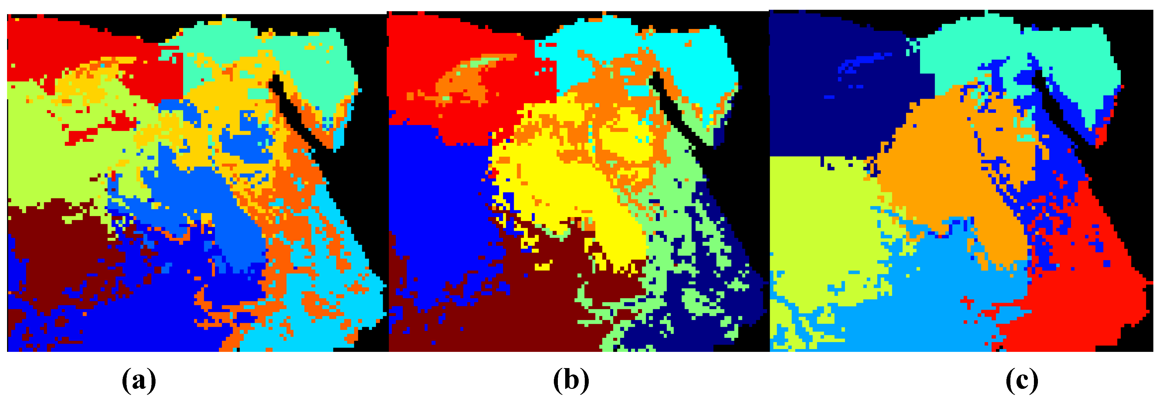
A 14-dimensional dataset was formed and the result of k-means clustering with increasing spatial influence is shown in
Figure 6. Nevertheless, clusters remain spatially relevant and the general placement of the cluster’s borders resembles the SRTM DEM of
Figure 1. Compared to the temporal clusters of
Figure 4, the seven spatiotemporal regions preserve spatial concentration.
Figure 6.
Spatially fused clustering with gradually ascending spatial weights (a) 1/7, (b) 1/5 and (c) 1/4. The progressive spatial connectivity is apparent.
Figure 6.
Spatially fused clustering with gradually ascending spatial weights (a) 1/7, (b) 1/5 and (c) 1/4. The progressive spatial connectivity is apparent.
Additionally, spatiotemporal clustering tying both temporal variations and pixel distances was considered. The multidimensional cluster space was four dimensional, including space (x, y), time (t) and temperatures. As temporal variance was incorporated into spatial proximity, clusters formed three-dimensional concentrated regions. Since scale and spread of data are highly unrelated, a normalization step forced all dimensions to become comparable. Weighted coordinate arrangement was supported to enhance or weaken temperature and temporal contributions.
Generalized visualization of the formed clusters revealed bulks of spatiotemporal similarities over the multi-temporal imagery (
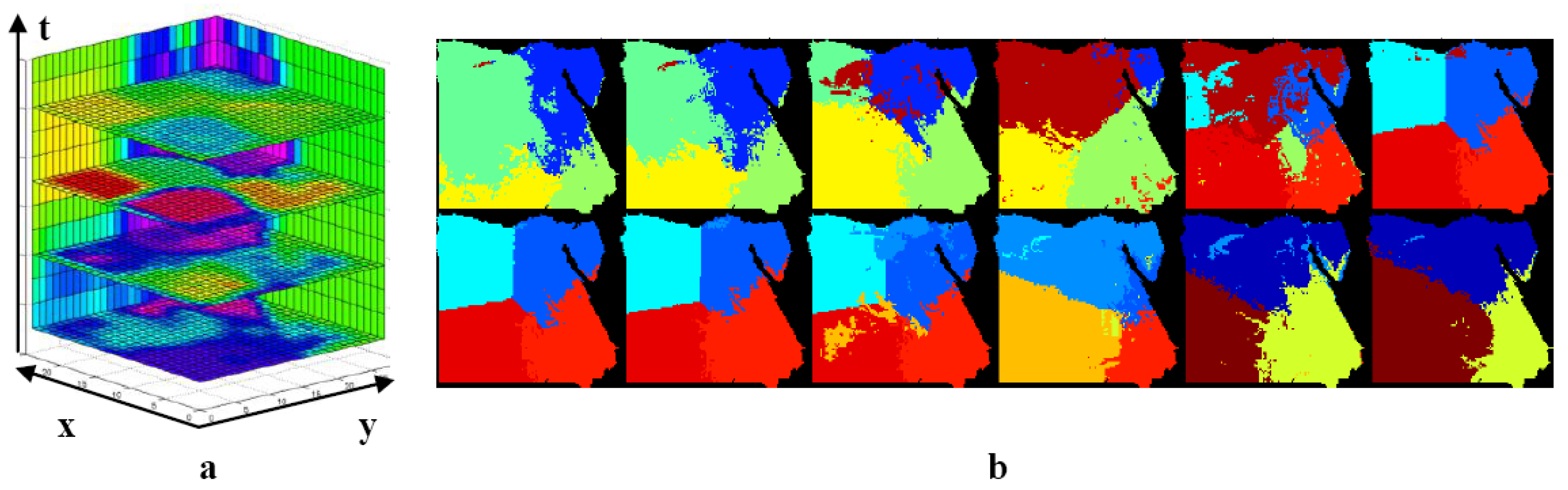
Figure 7(a)). The temporal axis (t) corresponds to the clustered scene snapshots of the first, fourth, seventh, and tenth months, while interpolated in-between scenes can be visualized. As seen in
Figure 7(b), clusters in many instances are regularly spaced indicating reduced temperature variability and thus resembling the area’s geomorphology. Nevertheless, cluster irregularities shown in various instances indicate areas of possible interest or temperature differentiation.
Figure 7.
(a) Visualizing colored bulks of three-dimensional clusters under spatiotemporal clustering, (b) 12 two-dimensional temporal slices from spatiotemporal clustering. Slices with irregularly dispersed clusters indicate temperature discrepancies.
Figure 7.
(a) Visualizing colored bulks of three-dimensional clusters under spatiotemporal clustering, (b) 12 two-dimensional temporal slices from spatiotemporal clustering. Slices with irregularly dispersed clusters indicate temperature discrepancies.
2.5. Elevation Biased Clustering
In the previous sections, clustering (
Figure 4) and spatially fused clustering (
Figure 6) were applied to LST data in an attempt to identify regions with common annual LST variation. On the other hand, geomorphology provides the framework for the interaction among various biophysical parameters, while planners, biologists, environmental scientists,
etc., consider landscape as the framework for the integration of spatial relationships. Towards this end, geomorphologic data were integrated to LST data in an elevation biased clustering process, with the advantage of producing a terrain dependent organization of annual LST variations. Such an approach would probably reveal annual LST differences among the regions with the same physiographic characteristics.
Elevation within each 0.05 degree MODIS LST pixel was computed as the mean of all SRTM elevation values in each MODIS pixel. K-means clustering was then performed based on 13 rasters: 12 monthly LST rasters and the elevation raster. The clustering algorithm merged clusters with less than 0.1 percent area into larger clusters and clustering stopped after less than 0.02 percent of the pixels changed class membership. Sixteen classes were output after 276 clustering iterations.
The cluster centroids are given in
Table 2 and in
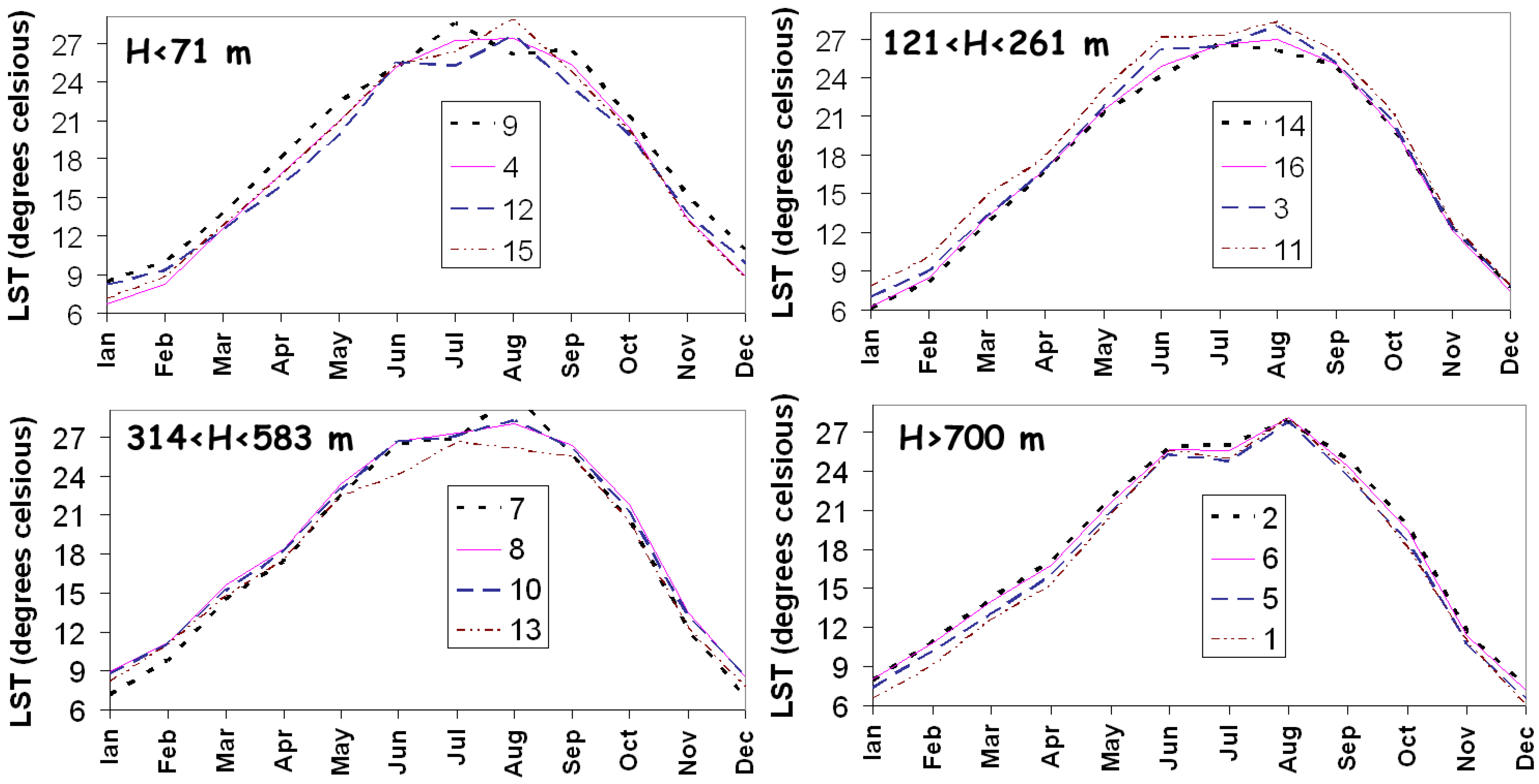
Figure 8. Note that clusters were sorted in increasing centroid elevation value (
Table 2) and grouped to 4 categories of mean (centroid) elevation (H), (a) < 71 m, (b) 121 < H < 261 m (c) 314 < H < 583, (d) H > 700 m. The occurrence and the H centroid statistics (mean and standard deviation of elevation) are presented in
Figure 9. Thus, the relief of Egypt was classified to four groups on the basis the 16 cluster centroids and within each group the annual LST variation is provided (
Figure 8). The interpretation of the spatial distribution (
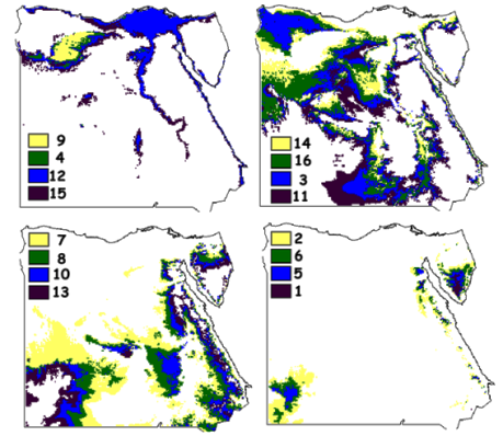
Figure 10) of the 16 clusters, grouped to four relief categories revealed annual LST differences among regions with common relief.
Table 2.
Cluster occurrence and centroids (elevation and LST per month). Note that clusters were sorted in increasing mean elevation (negative mean elevation indicate clusters occupied by the Alexandria Lake).
Table 2.
Cluster occurrence and centroids (elevation and LST per month). Note that clusters were sorted in increasing mean elevation (negative mean elevation indicate clusters occupied by the Alexandria Lake).
| Clus-ter ID | Occur-rence % | Elevation (m) | LST per Month (degrees Celsius) |
|---|
| Mean | S.D. | Jan | Feb | Mar | Apr | May | Jun | Jul | Aug | Sep | Oct | Nov | Dec |
|---|
| 9 | 1.5 | −74 | 15 | 8.4 | 9.9 | 13.8 | 18.1 | 22.5 | 25.1 | 28.5 | 26.1 | 26.5 | 21.4 | 15.1 | 11.0 |
| 4 | 0.9 | −21 | 14 | 6.7 | 8.2 | 12.5 | 16.8 | 21.0 | 25.2 | 27.1 | 27.3 | 25.3 | 20.4 | 13.4 | 8.9 |
| 12 | 7.0 | 19 | 13 | 8.2 | 9.3 | 12.4 | 15.9 | 19.8 | 25.5 | 25.2 | 27.6 | 23.6 | 19.8 | 13.7 | 9.9 |
| 15 | 4.9 | 71 | 15 | 7.1 | 8.8 | 12.7 | 16.6 | 20.8 | 25.3 | 26.3 | 28.8 | 24.7 | 20.1 | 13.2 | 8.7 |
| 14 | 7.4 | 121 | 13 | 6.1 | 8.2 | 12.7 | 16.8 | 21.3 | 24.1 | 26.6 | 26.1 | 24.9 | 19.9 | 12.4 | 7.7 |
| 16 | 11.7 | 163 | 13 | 6.3 | 8.5 | 13.2 | 16.8 | 21.5 | 24.8 | 26.5 | 27.0 | 25.1 | 20.1 | 12.1 | 7.5 |
| 3 | 13.2 | 209 | 14 | 7.0 | 9.0 | 13.3 | 16.8 | 21.7 | 26.1 | 26.4 | 28.0 | 25.1 | 20.3 | 12.3 | 7.7 |
| 11 | 11.0 | 261 | 15 | 7.8 | 10.1 | 14.8 | 17.8 | 23.0 | 27.0 | 27.2 | 28.3 | 25.9 | 21.1 | 12.7 | 7.9 |
| 7 | 13.9 | 314 | 18 | 7.1 | 9.7 | 14.6 | 17.4 | 22.6 | 26.4 | 26.8 | 30.4 | 25.6 | 20.6 | 12.1 | 7.0 |
| 8 | 8.8 | 394 | 23 | 9.0 | 11.1 | 15.6 | 18.4 | 23.4 | 26.6 | 27.3 | 28.0 | 26.3 | 21.8 | 13.4 | 8.5 |
| 10 | 7.0 | 477 | 27 | 8.7 | 11.1 | 15.2 | 18.1 | 23.0 | 26.6 | 27.1 | 28.3 | 26.0 | 21.2 | 13.2 | 8.4 |
| 13 | 5.5 | 583 | 31 | 8.1 | 10.9 | 14.7 | 17.5 | 22.4 | 24.1 | 26.6 | 26.1 | 25.5 | 20.4 | 12.3 | 7.8 |
| 2 | 3.8 | 700 | 38 | 7.9 | 10.9 | 14.2 | 17.0 | 21.9 | 25.8 | 25.9 | 27.8 | 24.9 | 19.8 | 11.6 | 7.4 |
| 6 | 1.8 | 858 | 50 | 8.0 | 10.9 | 13.9 | 16.7 | 21.6 | 25.6 | 25.6 | 28.1 | 24.4 | 19.4 | 11.3 | 7.2 |
| 5 | 1.1 | 1047 | 76 | 7.4 | 10.2 | 13.0 | 16.0 | 20.8 | 25.2 | 24.7 | 27.7 | 23.5 | 18.5 | 10.6 | 6.5 |
| 1 | 0.3 | 1452 | 217 | 6.5 | 9.0 | 12.6 | 15.2 | 20.6 | 25.5 | 24.9 | 28.0 | 23.9 | 18.1 | 11.0 | 6.0 |
Figure 8.
The LST centroids of the 16 clusters (
Table 2) organized into four categories in increasing mean elevation (H) (
Figure 10). The mean elevation (H) range per category is indicated in each figure.
Figure 8.
The LST centroids of the 16 clusters (
Table 2) organized into four categories in increasing mean elevation (H) (
Figure 10). The mean elevation (H) range per category is indicated in each figure.
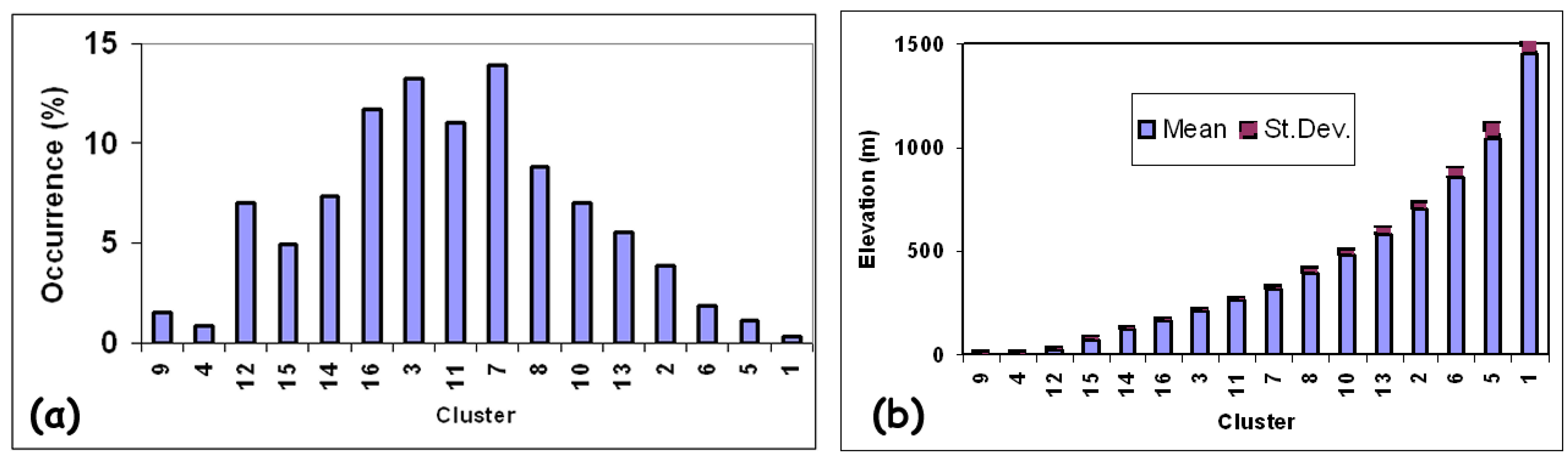
Figure 9.
(a) Percent area of each cluster class.
(b) Mean elevation within each cluster class. Clusters were sorted in increasing mean elevation (
Table 2).
Figure 9.
(a) Percent area of each cluster class.
(b) Mean elevation within each cluster class. Clusters were sorted in increasing mean elevation (
Table 2).
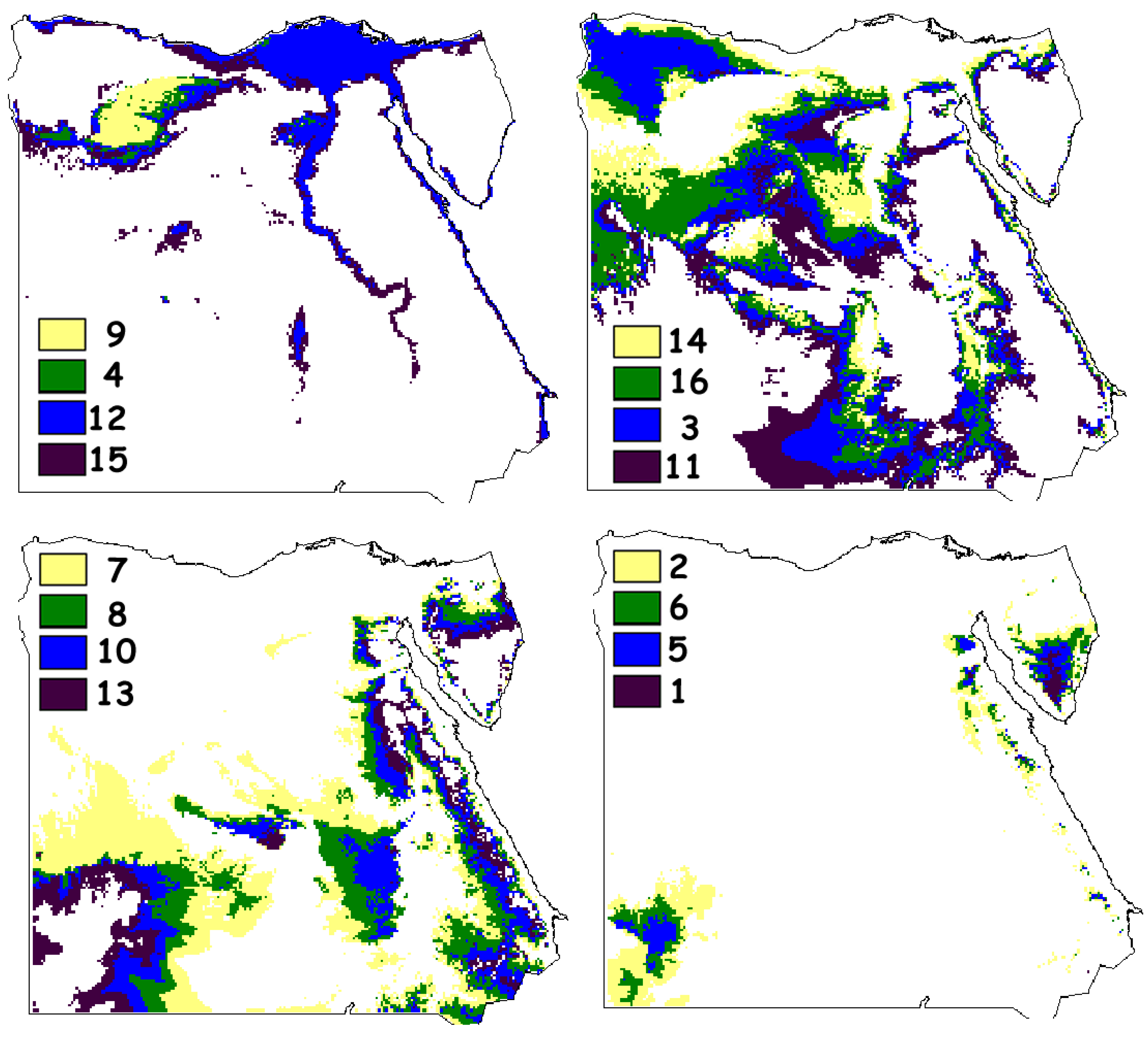
Figure 10.
The spatial distribution of the 16 clusters corresponding to the elevation biased clustering. The clusters were organized in four groups in increasing mean elevation according to
Figure 8. Both seasonal LST variations and the spatial distributions of regions with the same elevation range are revealed. Thus the most elevated clusters (2, 6, 5, 1) map the spatial extent of two regions with different annual LST variability in Sinai (NE) while in the lowland (clusters 9,4,12,15) LST differences are identified among regions in Nile Delta, Nile River, Alexandria Lake and the coastal zone in the north (Mediterranean Sea) and east (Red Sea).
3. Results and Discussion
The eight clusters presented more or less distinct centroids (
Figure 5,
Table 1), with specific spatial arrangement (
Figure 4), while the mean elevation of each cluster played a significant role (
Table 1,
Figure 3). The clusters were arranged in decreasing mean LST centroid co-ordinates order for the months May to September as follows: 7, 1, 8, 6, 3, 5, 4, 2 (
Table 1,
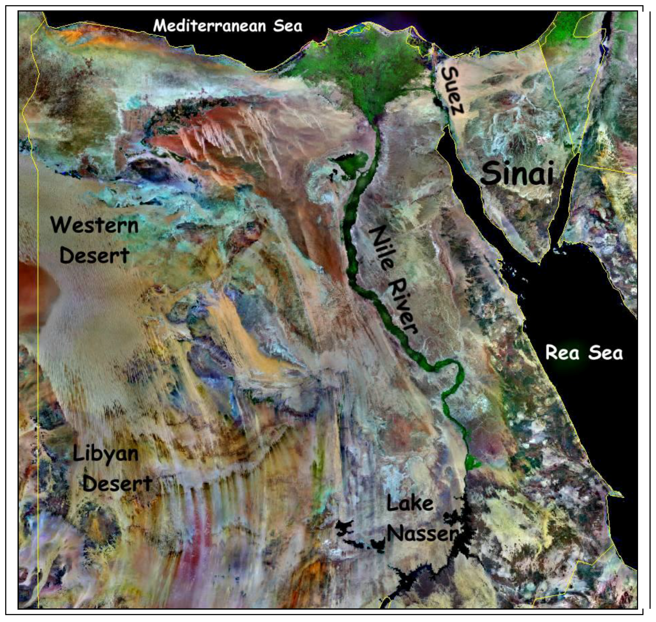
Figure 5). In order to assist interpretation, a satellite image map of Egypt [
16] is shown (
Figure 11) in which selective places of interest are identified.
Figure 11.
Orthorectified Landsat Thematic Mapper Mosaic [
16], Band 7 (mid-infrared light) is displayed as red, Band 4 (near-infrared light) is displayed as green, Band 2 (visible green light) is displayed as blue.
Figure 11.
Orthorectified Landsat Thematic Mapper Mosaic [
16], Band 7 (mid-infrared light) is displayed as red, Band 4 (near-infrared light) is displayed as green, Band 2 (visible green light) is displayed as blue.
Clusters 2 and 4 present the coolest centroids (
Figure 5,
Table 1). Cluster 2 corresponds to the low elevated (
Table 1,
Figure 3) plain (since standard deviation of elevation is minimized in
Table 1) north coastal region along the Mediterranean Sea (
Figure 4). Cluster 4 is located further south than Cluster 2, and occupies the most elevated (
Figure 3) and dissected (standard deviation of elevation is maximized in
Table 1) regions, for example the Sinai (
Figure 8), South-East of Suez Canal.
The warmest (
Figure 5) clusters (7, 1, 8, 6, and 3) are spatially distributed along east to west direction (
Figure 4). Clusters 7, 1 and 8 present almost similar elevation statistics (
Table 1,
Figure 3), with a mean elevation that is higher than the mean elevation of clusters 6 and 3. Cluster 5 (it is a rather cool cluster since its LST centroid approaches the centroids of clusters 2 and 4) is distributed almost uniformly all over the country. The high elevation (
Table 1,
Figure 3) of the regions forming cluster 5 interprets the behavior of the corresponding LST centroid, while a portion of Nile River is also interpreted to belong to cluster 5 (
Figure 4).
Each of the 16 clusters derived by the elevation biased clustering were formed by regions with almost common elevation range as it was concluded by the standard deviation of clusters centroid (
Figure 9,
Table 2).
The category that includes the most elevated clusters 2, 6, 5, 1 is formed by the Sinai Mountains in the NE and the elevated region in SW according to
Figure 10. The 4 LST centroids (
Figure 8) for this group indicate a variation of the annual LST that is elevation dependent. The four lowest in elevation clusters (9, 4, 12, 15) are grouped in a category that includes the coastal regions along the Mediterranean Sea, Red Sea, Alexandria Lake (clusters 4 and 9 with negative elevation centroid) as well as the Nile Delta (
Figure 10). The four LST centroids (
Figure 8) for this group indicate a variation of the annual LST that depends on the proximity to inland waters and sea as well as latitude.
For the two groups of intermediate elevation (a) 121 to 261 m and (b) 314 to 583 m (
Table 2,
Figure 10), it is concluded that the lower elevated group is represented by a cooler annual LST curve (
Figure 8), due to its proximity to the sea and the Nile River. The four LST centroids (
Figure 8) for each group, indicate a variation of the annual LST that is elevation dependent.
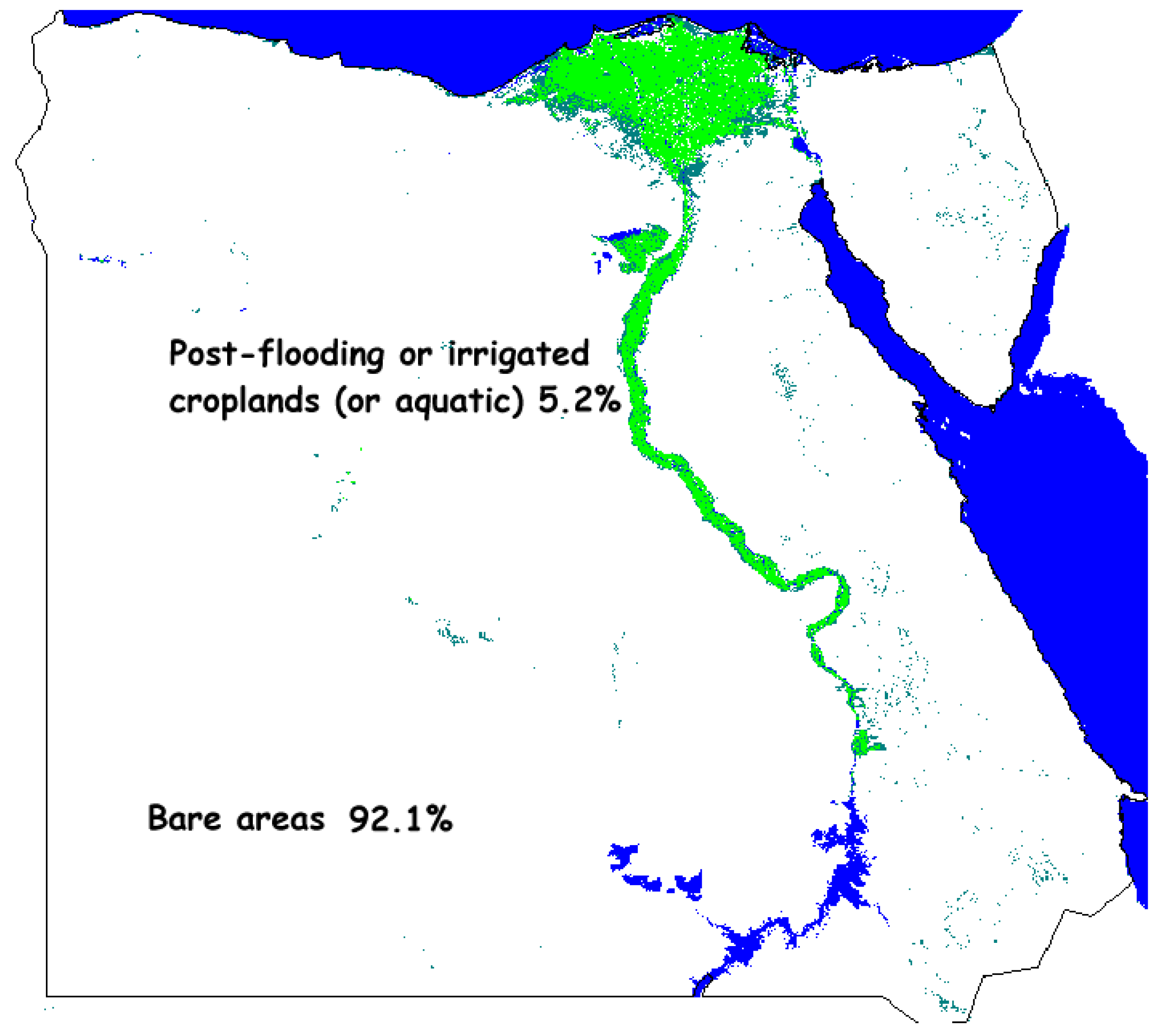
The GlobCover landcover map, available from the European Space Agency Ionia Portal (
http://ionia1.esrin.esa.int/) was used to identify the major landcover classes in Egypt. It was developed using as input observations from the 300m MERIS sensor on board the ENVISAT satellite mission over a period of 19 months (December 2004–June 2006). The majority of Egypt is occupied by two landcover classes (a) bare area (92.1) and (b) post-flooding or irrigated croplands or aquatic (5.2%), with the last one corresponding mainly to cluster 12 (
Table 2,
Figure 10,
Figure 12).
Figure 12.
The GlobCover (© ESA/ESA GlobCover Project, led by MEDIAS-France) lancover map of the study area.
Figure 12.
The GlobCover (© ESA/ESA GlobCover Project, led by MEDIAS-France) lancover map of the study area.
4. Conclusions
Thermal terrain segmentation from multi-temporal monthly night imagery outlined objectively both the temporal variation of LST during 2006 and the spatial distribution of LST zones. The Northern coastal region along the Mediterranean Sea, occupied by lowland plain areas, corresponded to the coolest clusters indicating a latitude/elevation dependency of seasonal LST variability. On the other hand for the inland regions, elevation and terrain dissection play a key role in LST seasonal variability, while an East to West variability of clusters’ spatial distribution was revealed. Finally, the elevation biased clustering revealed annual LST differences among the regions with the same physiographic/terrain characteristics.
Mapping of regions with common annual LST variability would assist planning, decision making and climatic change studies at moderate resolution scale. The derived Egypt’s LST signatures could provide a tool for environmental assessment comparison and evaluation between different countries.


