Determination of Backscatter-Extinction Coefficient Ratio for LIDAR-Retrieved Aerosol Optical Depth Based on Sunphotometer Data

Abstract

Backscattered power data from the Doppler LIght Detection And Ranging (LIDAR) systems at the Hong Kong International Airport (HKIA) could be used to obtain the extinction coefficient of the troposphere by combining with the meteorological optical range (MOR) data from the nearby forward scatter sensor. The Range-height Indicator (RHI) scan of the LIDAR is then utilized to derive the vertical profile of extinction coefficient, which is integrated with height to obtain the aerosol optical depth (AOD). In the retrieval of extinction coefficient profile, there is a power exponent of unknown value relating the backscattered power and the extinction coefficient. This exponent (called the backscatter-extinction coefficient ratio) depends on the optical properties of the aerosol in the air, and is normally assumed to be 1. In the present study, the value of this ratio is established by comparing the AOD measurements by a hand-held sunphotometer and the LIDAR-based AOD estimate in one winter (October 2008 to January 2009), which is the season with the largest number of haze episodes, and one summer-winter-spring period of the following year (July 2009 to May 2010) at HKIA. It is found to be about 1.4. The sensitivity of extinction coefficient profile to the value of the ratio is also examined for two cases in the study period, one good visibility day and one hazy day.

1. Introduction

Aerosol optical depth (AOD) data are useful in the monitoring of hazy weather. Such data can be obtained from meteorological satellite observations (e.g., Moderate Resolution Imaging Spectroradiometer, MODIS) and ground-based LIDAR data [1]. At the Hong Kong International Airport (HKIA), two Doppler LIDAR systems of the Hong Kong Observatory (HKO) have been in operation for windshear alerting. At the same time, the backscattered power data from the LIDAR, coupled with the meteorological optical range (MOR) readings from the nearby forward scatter sensors, could be used to retrieve the vertical profile of extinction coefficient, which is integrated with height to give the AOD.

In retrieving the extinction coefficient profile using Klett’s method ([1,2]), it is assumed that the backscatter coefficient β is related to the extinction coefficient σ through a power law, namely, β α σ^k. The power index k, which is called backscatter-extinction coefficient logarithmic ratio or backscatter-extinction coefficient ratio in short in this paper, is unknown theoretically and dependent on the optical properties of the aerosol in the air. It is common to assume that k = 1. However, there are many studies based on LIDAR measurements that k may not be equal to 1. For instance, in a study at Lanzhou, China, k is found to be 0.8–0.9 (see [3]). LIDAR observations of aerosol have been made in Hong Kong, and some observations are reported in [4,5,6].

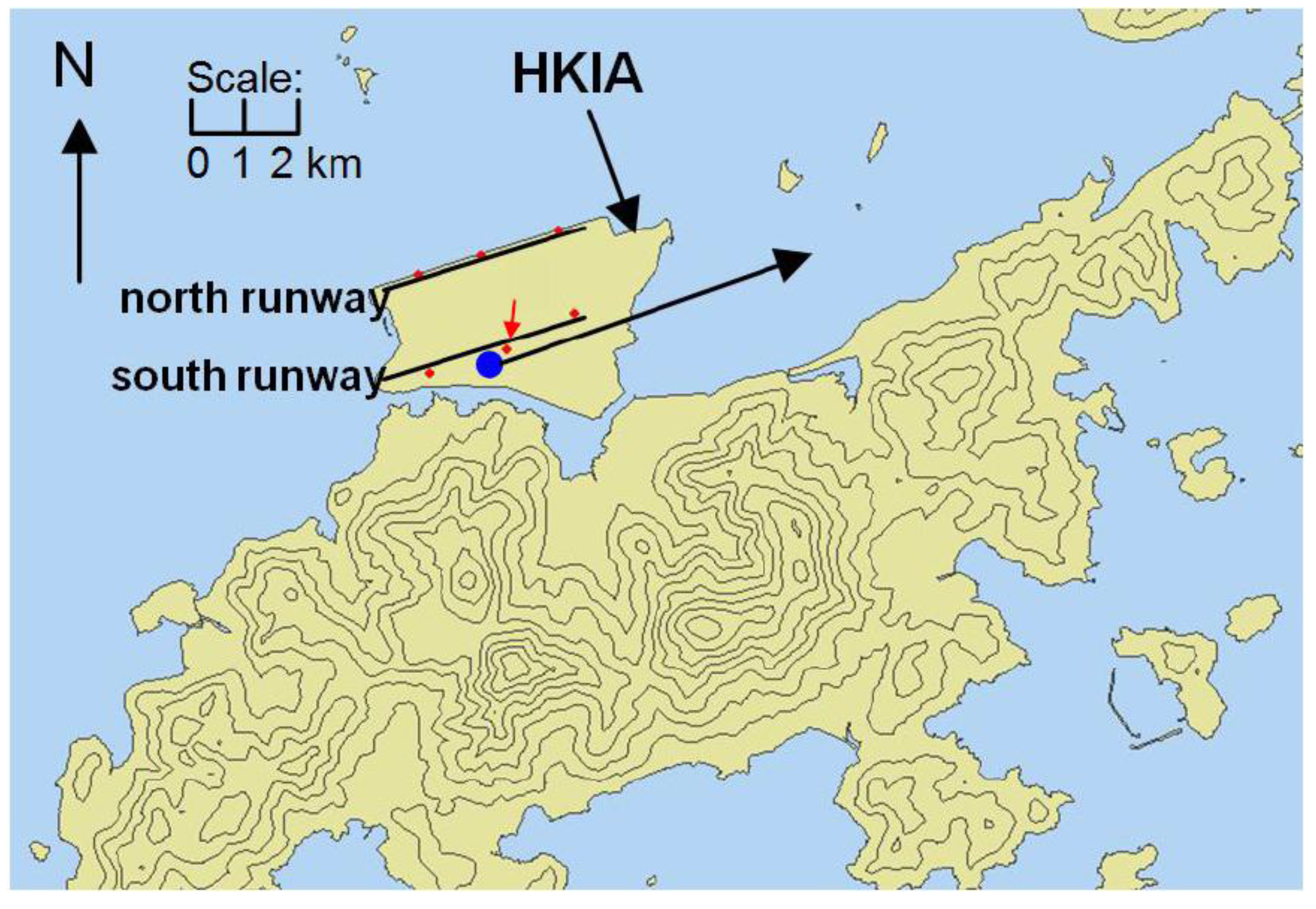
The value of k is established in this paper using AOD measurements of a hand-held sunphotometer (Microtops II) as ground truth. As the sunphotometer has not been used at HKIA for a long time, only the data of one winter (October 2008 to January 2009), which is the season with the highest number of hazy days, and one summer-winter-spring (July 2009 to May 2010) are considered in this paper. Only the data from the south runway LIDAR (location in Figure 1) are considered in the present study. The backscattered profiles are taken from Range-height Indicator (RHI) scans at an azimuth angle of 70 degrees from the north, as shown by the arrow in Figure 1. The LIDAR data are combined with the MOR readings from the forward scatter sensor near the center of the south runway (location in Figure 1) in retrieving the extinction coefficient profile.

Figure 1. Location of the LIDAR (blue dot) and the direction of the LIDAR RHI scans considered in the present study. The red dots indicate the locations of the forward scatter sensors along the two runways. The forward scatter sensor used in the study is indicated by a red arrow.

Figure 1. Location of the LIDAR (blue dot) and the direction of the LIDAR RHI scans considered in the present study. The red dots indicate the locations of the forward scatter sensors along the two runways. The forward scatter sensor used in the study is indicated by a red arrow.

2. Calculation of AOD

The calculation methodology is the same as that in [1] and only a summary of the major equations is given here. The distance-corrected backscattered power S of the LIDAR could be used to retrieve the extinction coefficient profile of the troposphere using Klett’s method based on the following equation:

$$\sigma (r)=\frac{\exp [(S(r)-S_m)/k]}{\left\{{\sigma }_m^{-1}+\frac{2}{k}{\displaystyle \underset{r}{\overset{r_m}{\int }}\exp [(S(r\prime )-S_m)/k]dr\prime }\right\}}$$

(1)

where those quantities with subscript m are the corresponding values at a reference distance. The extinction coefficient σ for the LIDAR’s wavelength (2,022 nm) is adjusted to that at the visible range (500 nm), indicated as σ’. The latter quantity is then integrated with height to give AOD:

$$AOD={\displaystyle \underset{0}{\overset{z_{\max }}{\int }}\sigma \prime (z)dz}$$

(2)

Following [1], the maximum height z_max is taken to be 4 km.

The LIDAR in use in the present study is calibrated for the radial velocity and it is not calibrated for the backscattered power. As such, the backscattered data from the LIDAR shows the relative variation of the aerosol concentration (in case of haze) in the troposphere. The accuracy of the LIDAR-derived AOD would then depend on that of the meteorological optical range (MOR) measurement from the forward scatter sensor in use. For the model considered at HKIA (FD-12P at Vaisala), the accuracy of MOR is within 10% for visibility less than 10 km. The performance of Microtops II in the determination of AOD has been studied in [7]. The same model of sun photometer has been used at HKIA. It has been calibrated at the factory before being used in Hong Kong. According to the manufacturer, the AOD measurement from Microtops II has an accuracy of 0.01.

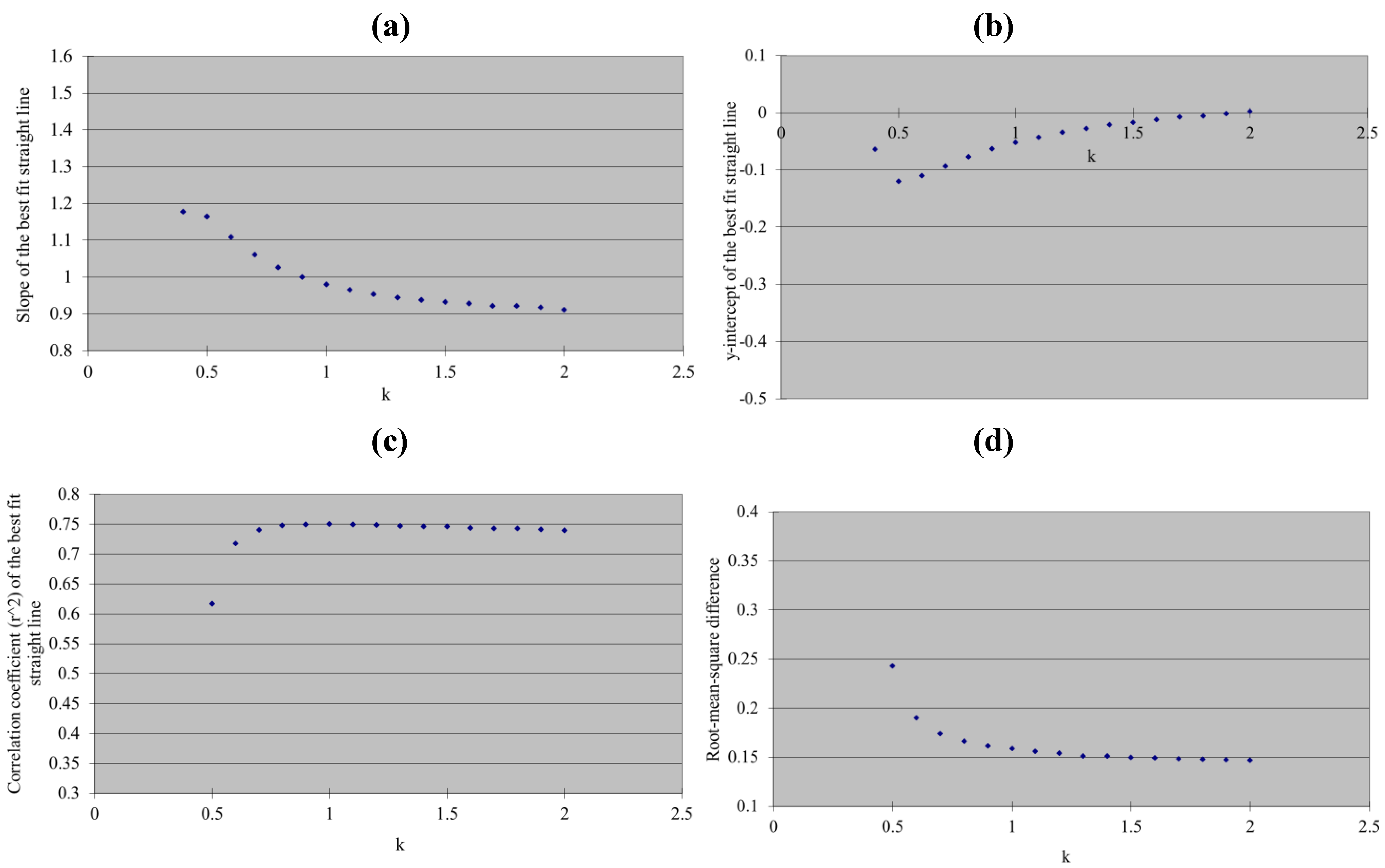
3. Selection of k Based on Data from October 2008 to January 2009

The AOD values calculated from the LIDAR are compared with the actual measurements from the sunphotometer. In the LIDAR retrieval, the ratio k is varied between 0.5 and 2.0 at a step of 0.1. For each value of k, the LIDAR AOD is plotted against the sunphotometer AOD for the whole study period and the data points are fitted with a straight line using total least square technique (as in [1]). Three quantities of the best-fit straight line are considered, namely, the slope, y-intercept and correlation coefficient (R²). Moreover, the root-mean-square (r.m.s.) difference between the two AOD datasets is considered.

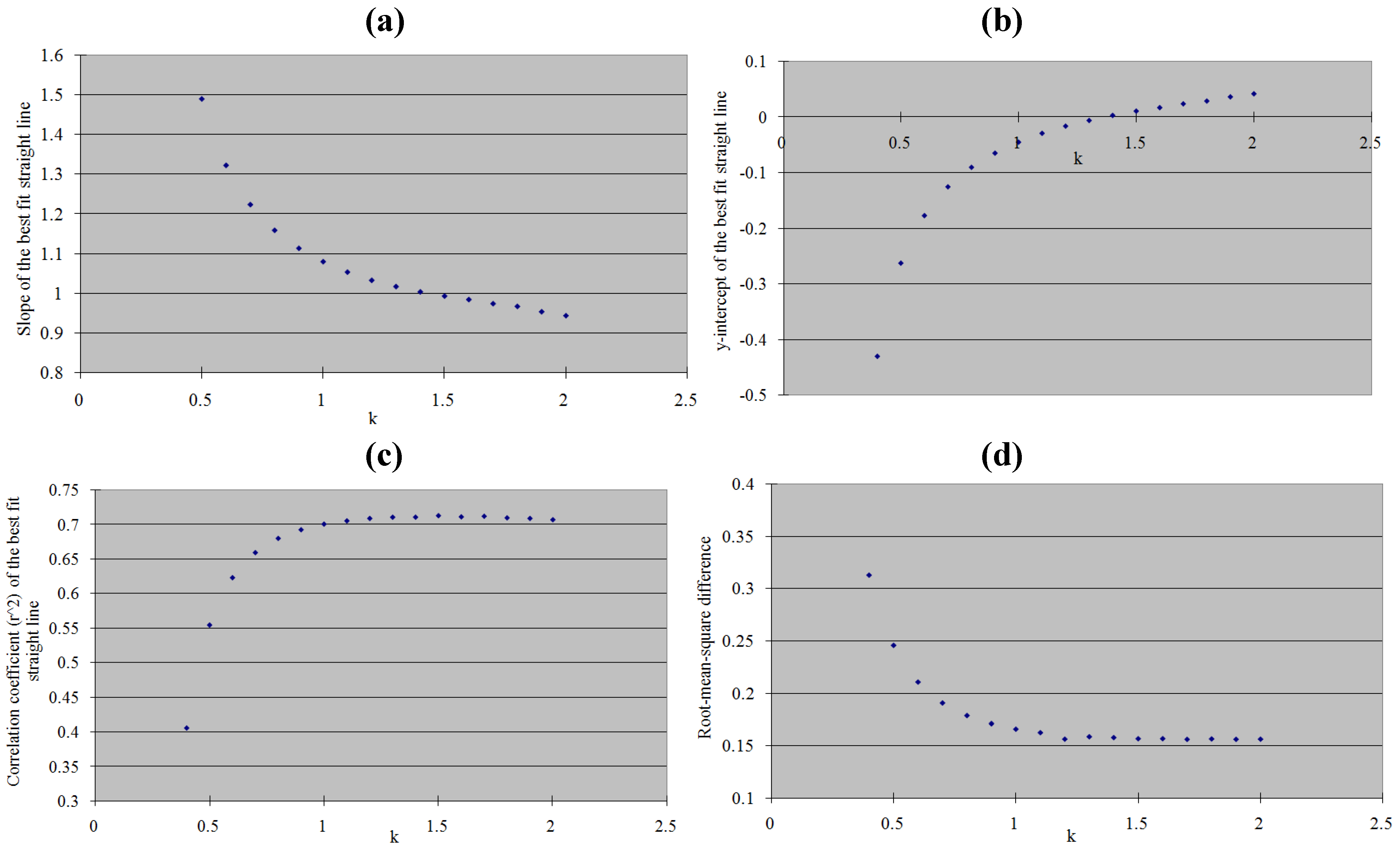
The variations of the above-mentioned quantities with k are shown in Figure 2(a–d). The slope of the best fit straight line is closest to 1 and the corresponding y-intercept is closest to 0 for k = 1.4. The R² and r.m.s. difference also flat out with k for k ≥ 1.2. As such, the optimum value of k for the airport area is about 1.4, at least based on the data in the study period (October 2008 to January 2009).

Figure 2. Variation of the following quantities with k: (a) slope, (b) y-intercept, and (c) correlation coefficient of the best fit straight line, and (d) root-mean-square difference, between AOD from LIDAR and AOD from sun photometer during the period October 2008 to January 2009.

Figure 2. Variation of the following quantities with k: (a) slope, (b) y-intercept, and (c) correlation coefficient of the best fit straight line, and (d) root-mean-square difference, between AOD from LIDAR and AOD from sun photometer during the period October 2008 to January 2009.

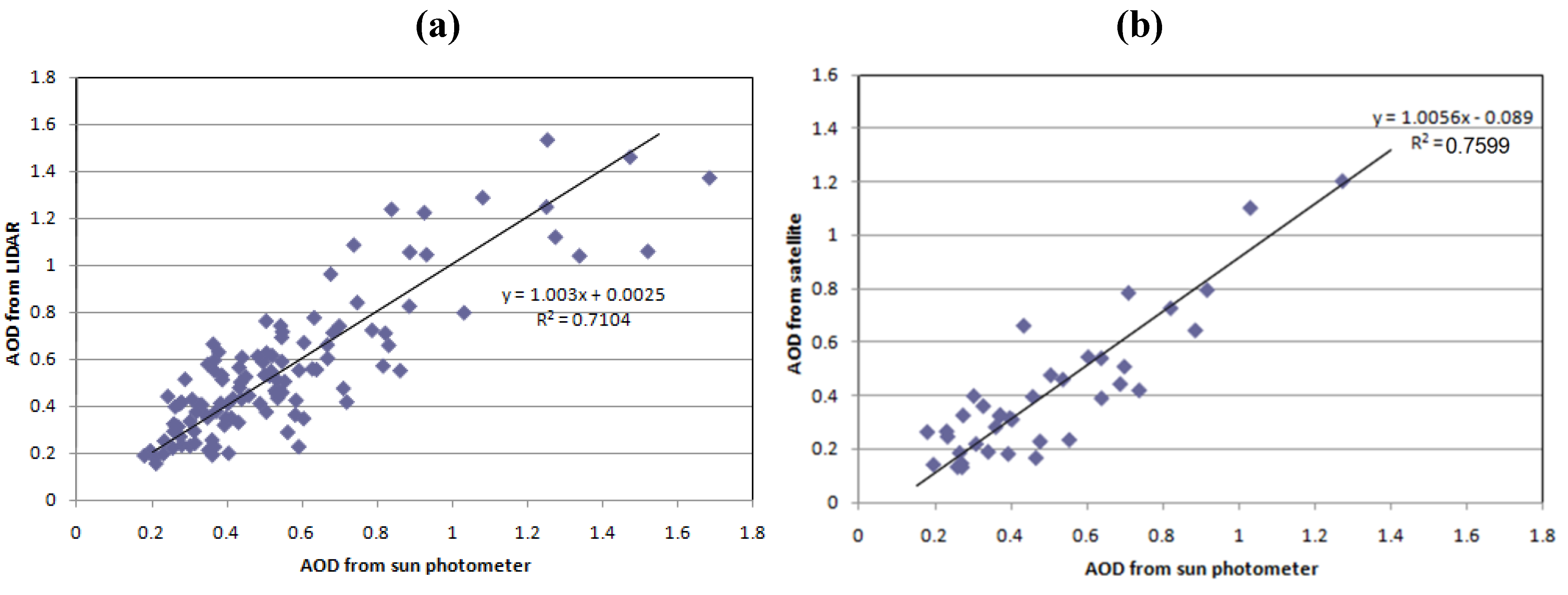
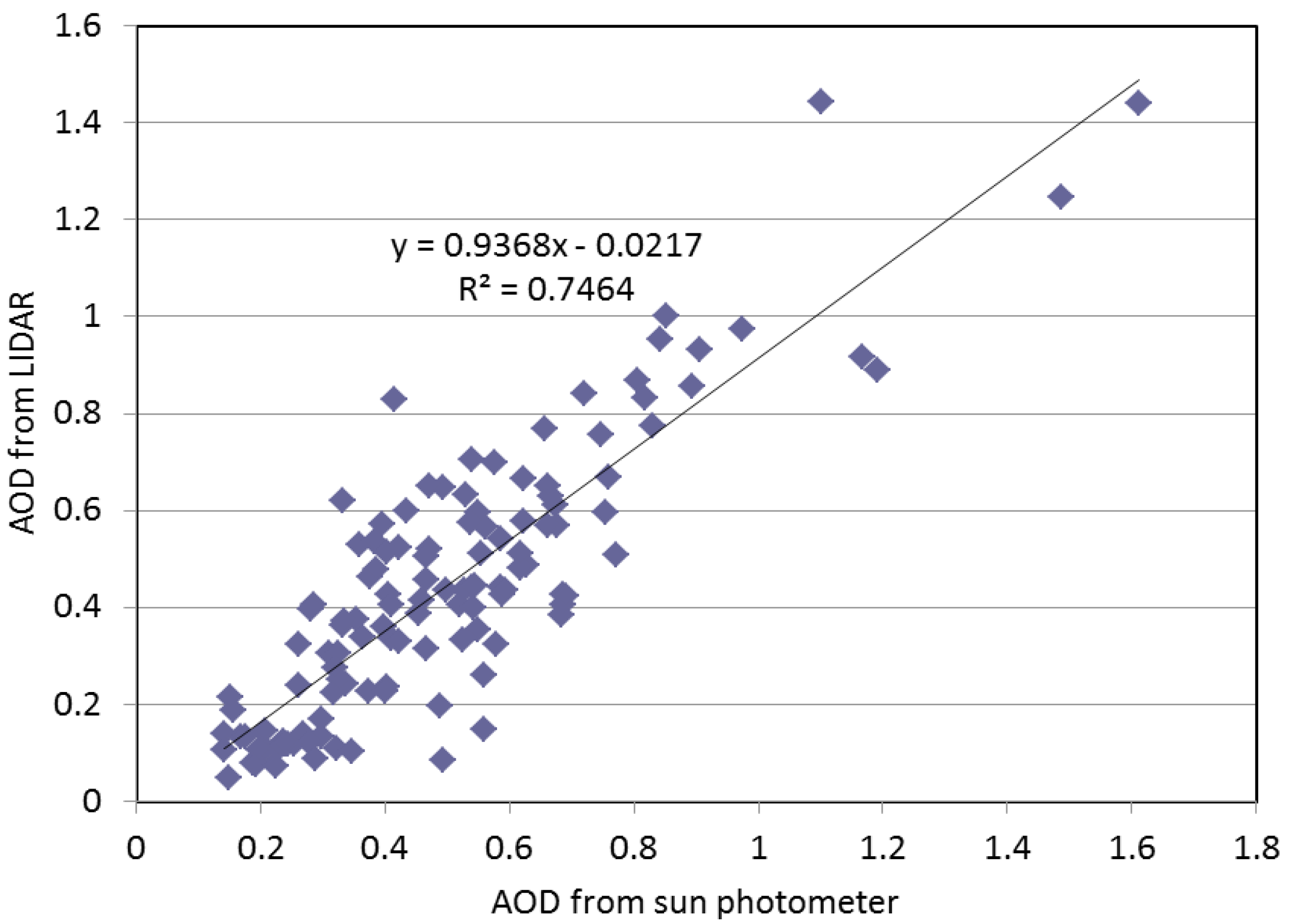
The AOD data points and the best fit straight line at k = 1.4 are shown in Figure 3(a). As a comparison, the corresponding scatter plot for MODIS AOD vs. sunphotometer AOD is given in Figure 3(b) (note: study period is the same but the actual observation times may be different because Figure 3(b) only includes those data points when MODIS AOD data are available). The slopes and the y-intercepts of the best fit straight lines in Figure 3(a,b) are of similar magnitude. The R² for MODIS is higher, but of a magnitude comparable with that for LIDAR.

For the cases under consideration in the present study, there does not seem to be any signal of suspending aerosols above 4 km from the LIDAR’s backscattered data. As such, though integration is only made up to 4 km above ground, the LIDAR-based AOD is expected to have a magnitude comparable with, instead of smaller than, that measured by the sunphotometer. As a result, the optimal value of k is determined based on, among others, the closeness of the slope of the best-fit straight line to unity by considering all the slopes above and below unity, instead of focusing on those slope values below unity only. In fact, for the optimal value of k = 1.4, the slope is just 1.003, which is very close to 1.

Figure 3. Scatter plot of AOD: (a) between LIDAR and sun photometer, and (b) between MODIS and sun photometer.

Figure 3. Scatter plot of AOD: (a) between LIDAR and sun photometer, and (b) between MODIS and sun photometer.

4. Selection of k Based on Data from July 2009 to May 2010

The comparison study in Section 3 has been repeated for the longer period of time in the next year, namely, between July 2009 and May 2010, covering more seasons (summer, winter to the spring of the next year). The objective is to find out if the optimal value of k determined in the previous year could be applicable in the next year and over other seasons as well.

From the slope of the best-fit straight line between LIDAR-measured AOD and sunphotometer-measured AOD (Figure 4(a)), it is closest to unity for k in the order of 0.9. However, for larger values of k, the slope still does not deviate significantly from unity. For instance, for k = 1.4, the slope is about 0.94.

From the y-intercept of the best-fit straight line (Figure 4(b)), it is closer to zero when the k value is larger, approaching 2.0. For k in the region of 1.4, the y-intercept is about -0.02, which is already rather small.

From the correlation coefficient of the data points to the best-fit straight line (Figure 4(c)), it reaches a maximum value of about 0.75 for k = 0.8 or above. There are some fluctuations in the value of the correlation coefficient for lager values of k, but such changes are not considered to be significant.

From the r.m.s. difference between the two sets of data (Figure 4(d)), it reaches a minimum value of about 0.15 for k = 1.3. Again, there are some fluctuations in the r.m.s. difference value for larger values of k, but such changes do not appear to be significant.

Balancing all the factors, it appears that k = 1.4 could still be considered as an optimal value. The corresponding plot between LIDAR-derived AOD and sunphotometer-measured AOD can be found in Figure 5. Data collection is ongoing at HKIA. Further studies would be conducted in the future to see the variation of the optimal value of k in more years as well as the seasonal variation of this value.

Figure 4. Variation of the following quantities with k: (a) slope, (b) y-intercept, and (c) correlation coefficient of the best fit straight line, and (d) root-mean-square difference, between AOD from LIDAR and AOD from sun photometer during the period July 2009 to May 2010.

Figure 4. Variation of the following quantities with k: (a) slope, (b) y-intercept, and (c) correlation coefficient of the best fit straight line, and (d) root-mean-square difference, between AOD from LIDAR and AOD from sun photometer during the period July 2009 to May 2010.

Figure 5. Scatter plot of the LIDAR-derived AOD and sunphotometer-measured AOD in the period July 2009 to May 2010.

Figure 5. Scatter plot of the LIDAR-derived AOD and sunphotometer-measured AOD in the period July 2009 to May 2010.

As a preliminary study of the seasonal and year-to-year variability in the relationship between LIDAR-derived AOD and sunphotometer-measured AOD, the slope of the best-fit straight line for the two datasets is considered in different seasons with sufficiently large samples, namely, samples of at least 30. This sample requirement is only fulfilled in autumn 2008 (September to November), winter 2008 to 2009 (December to February next year), autumn 2009, and winter 2009 to 2010. The results are summarized in Table 1. It can be seen that there are variations in the values of the slopes, varying between 0.72 and 1.01. Given the limited amount of data available, it could not be concluded which season has the “best” result in terms of the slope being closest to unity. But year-to-year variability in the slope of the best-fit straight line can be seen, which may be related to the characteristics of the aerosols. With the accumulation of more data, such variability could be studied by comparing, for example, the chemical composition of the aerosols.

Table 1. Summary of the slope of the best-fit straight line between LIDAR-derived AOD and sunphotometer-measured AOD in different seasons. Only those periods with more than 30 samples are considered. The value of k = 1.4 is used.

Period	Slope	Number of samples
autumn 2008	0.736	53
winter 2008 to 2009	0.953	61
autumn 2009	1.011	46
winter 2009 to 2010	0.723	36

Table 1. Summary of the slope of the best-fit straight line between LIDAR-derived AOD and sunphotometer-measured AOD in different seasons. Only those periods with more than 30 samples are considered. The value of k = 1.4 is used.

Period	Slope	Number of samples
autumn 2008	0.736	53
winter 2008 to 2009	0.953	61
autumn 2009	1.011	46
winter 2009 to 2010	0.723	36

5. Sensitivity of Extinction Coefficient Profile to k

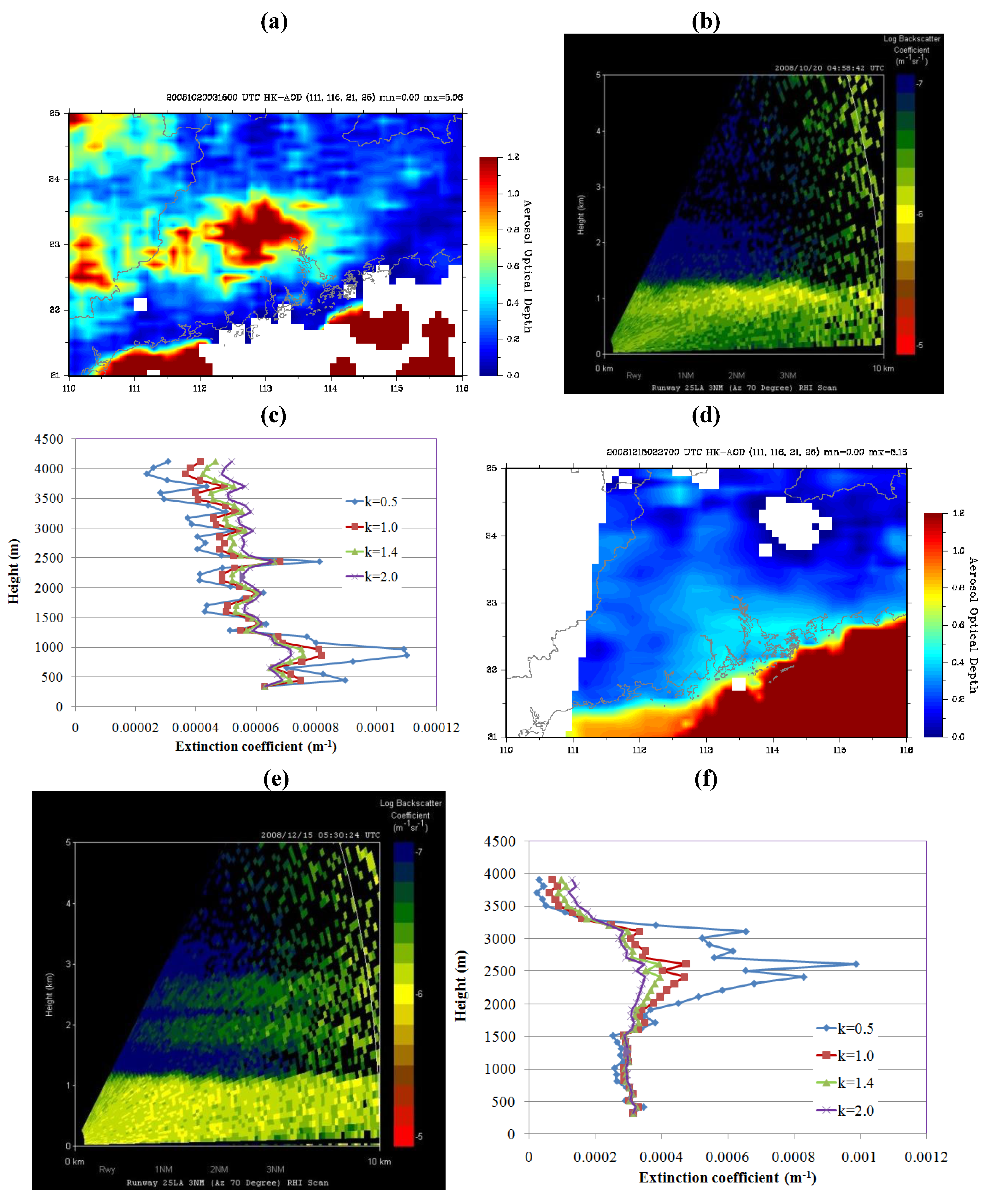
To demonstrate the sensitivity of extinction coefficient profile to the choice of k, two case studies have been conducted. The first occurs in the morning of 20 October 2008. At that time, visibility was good at HKIA and the human-observed visibility value was about 15 km. MODIS data show that AOD is relatively low along the coast of south China (Figure 6(a)), in the region of 0.1 to 0.2 only. Visibility in the region was in the order of 12–18 km. RHI scan of the LIDAR indicates that the backscattered power (and thus aerosol loading of the air) is higher from the ground up to around 1.1 km above (Figure 6(b)). The corresponding extinction coefficient profiles based on different values of k are given in Figure 6(c). It could be seen that the profiles for different k values have generally similar appearance. In particular, the extinction coefficient is higher below 1 km or so. However, the fluctuations of σ’ with altitude are more “exaggerated” for smaller value of k. As such, the AOD based on a smaller value of k (such as 0.5, with an AOD value of about 0.23) deviates more significantly from the sunphotometer measurement (about 0.28).

Similar behavior is also observed on a hazy day. During the daytime of 15 December 2008, it remained hazy at HKIA with the visibility hovering around 4000 m due to the aerosols brought about by the northwesterly sea breeze. MODIS data show that AOD is higher around the Pearl River Estuary compared with the inland areas of southern China (Figure 6(d)). RHI scan of the LIDAR (Figure 6(e)) indicates that, apart from the higher backscattered power values below 1.1 km or so, there are two elevated bands of higher values as well at about 2 km and 2.5 km above the sea level. As such, the retrieved σ’ does not drop significantly with altitude until at about 3 km. Once again, the σ’ profile (Figure 6(f)) shows more exaggerated fluctuations with height for a smaller value of k, particularly between 2 and 3.3 km (for k = 0.5). Thus, the resulting AOD value (1.37 for k = 0.5) deviates more from the sunphotometer measurement (1.25).

Figure 6. Data plots for the two events under study in this paper, namely, 20 October 2008: (a) MODIS AOD map at 03:16 UTC, 20 Oct 2008, (b) LIDAR RHI plot of backscattered power, (c) LIDAR-derived extinction coefficient profiles, and 15 December 2008: (d) MODIS AOD map at 02:27 UTC, 15 Dec 2008, (e) LIDAR RHI plot of backscattered power, (f) LIDAR-derived extinction coefficient profiles.

Figure 6. Data plots for the two events under study in this paper, namely, 20 October 2008: (a) MODIS AOD map at 03:16 UTC, 20 Oct 2008, (b) LIDAR RHI plot of backscattered power, (c) LIDAR-derived extinction coefficient profiles, and 15 December 2008: (d) MODIS AOD map at 02:27 UTC, 15 Dec 2008, (e) LIDAR RHI plot of backscattered power, (f) LIDAR-derived extinction coefficient profiles.

6. Conclusions

Based on the limited dataset in the present study, the backscatter-extinction coefficient ratio is found to have an optimum value of 1.4, at least for the winter of 2008–2009 and for the summer-winter-spring of 2009–2010. This is established by considering the RHI scan of a Doppler LIDAR and the MOR measurement by a nearby forward scatter sensor. The sunphotometer data are taken as the truth of AOD in the establishment of the optimal value of k. Data of two years have been considered, and as such it is believed that the optimal value of k so determined is quite representative of the condition at HKIA.

More sunphotometer data would be collected to study the seasonal and possibly the year-to-year variation of k. Furthermore, the impact of the different choices of k on the climatology of the LIDAR-based visibility map [8] would also be considered.