Meteorological Influence on Predicting Air Pollution from MODIS-Derived Aerosol Optical Thickness: A Case Study in Nanjing, China

Abstract

Whether the aerosol optical thickness (AOT) products derived from MODIS data can be used as a reliable proxy of air pollutants measured near the surface depends on meteorological influence. This study attempts to assess the influence of four meteorological parameters (air pressure, temperature, relative humidity, and wind velocity) on predicting air pollution from MODIS AOT data for the city of Nanjing, China. It is found that PM₁₀ (particulate matter with a diameter <10 μm) is linearly predictable from AOT at R² = 0.438. Seasonally, the prediction accuracy is much higher in summer (R² = 0.749, n = 24) and autumn (R² = 0.634, n = 45), but much lower in spring and winter (R² < 0.3). Scatterplots of the four meteorological parameters versus the residuals of PM₁₀ estimates from AOT reveal no definite relationship between them. Thus, the seasonality of any parameters cannot account for the variation in the prediction accuracy. Stepwise regression analysis reveals that air pressure (R² = 0.268) is the most important factor affecting the residuals of PM₁₀ (ΔPM₁₀) estimates in summer. In winter, the most important parameters are air pressure and air temperature (R² = 0.278). This accuracy rises to 0.510, similar to 0.409 for the summer season, if all four parameters are used in modeling ΔPM₁₀. However, no such models can be established for spring and autumn. It is concluded that meteorological parameters exert a mixed influence on the predictability of air pollution from AOT in the study area where air pollutants are dominated by suspended particulates.

1. Introduction

Air pollution is a serious environmental issue that has caused grave consequences, including rises in respiratory diseases, worsened health conditions for the elderly, and traffic delays due to poor visibility in developing countries such as China. Air quality in most Chinese cities has deteriorated rapidly over the last three decades during which the national economy started to boom. Rapid industrialization, popularization of private vehicles, and a booming construction sector have contributed to an exponential increase in suspended particulates in the atmosphere. Poor air quality has disrupted social harmony and hindered economic development in China [1].

In order to effectively control and solve the problem of air pollution, it is vitally critical to firstly monitor it over a long period. Regular monitoring of air quality is usually accomplished by recording crucial atmospheric constituents, such as particulate mass at a diameter of 10 micron or PM₁₀ at surveillance stations. Such ground-based observations, however, are limited in that the measurement is confined to the near surface, and hence unable to realistically depict pollutant concentrations in a column. Besides, the readings are obtainable at certain spots. When such point-based observations are extrapolated into a spatial region, errors are inevitably introduced to the interpolated pattern, especially when this pattern is not so predictable. These limitations, however, can be successfully overcome by means of remote sensing. Satellite imagery of a fine temporal resolution is able to yield timely information on the atmospheric conditions at the regional and global scales inexpensively, even though this method of estimation itself is subject to uncertainty. The advent of space-borne sensors designed specifically to study the atmospheric composition such as the MODerate resolution Imaging Spectroradiometer (MODIS) imagery, has considerably expanded the range of remotely sensed data useful for gathering air quality indicators, including aerosols. In monitoring air pollution, remote sensing complements ground-based observation by extending its limited coverage to a broad scale [2]. Space-borne imagery has been used increasingly for monitoring urban air quality [3]. The huge quantity of remotely sensed data accumulated so far create a potential for monitoring air pollution in urban areas and studying its long-term trend of variation.

The fine temporal resolution (12 hours) of MODIS imagery is perfectly suited to study solid atmospheric impurities such as aerosols that tend to change constantly. MODIS imagery has a proven capability in monitoring air pollutants at various spatial scales [4,5]. In conjunction with ground observations, MODIS data can be processed to derive accurate information on air pollutants for the entire state of Texas [6]. Remote sensing of air quality from satellite imagery requires an empirical relationship between reflectance of individual bands and concurrently collected in situ measurements of air pollution indicators, through which the satellite imagery is converted to maps of aerosol optical thickness (AOT). MODIS-derived AOT was found to bear a close relationship with ground observed particulate concentrations [7,8]. Daily mean concentration level of particulate matter is correlated with AOT at a statistically significant level. A close correlation (r = 0.7) exists between satellite-derived AOT and fine particulate mass or PM_2.5 [8,9]. This correlation may enable the determination of urban air pollution from the MODIS-derived AOT products. Comparison of such products with the corresponding data obtained with a sunphotometer convinced Li et al. [10] of the feasibility of studying air pollution from AOT. Satellite imagery can indeed serve as a reliable alternative in efficiently monitoring the spatial distribution of particulate pollutants at the ground level provided that special correction has been done to the imagery [11].

Nevertheless, it must be acknowledged that MODIS-derived AOT is not always a reliable surrogate of PM if air pollutants are not dominated by suspended particulates. In this case the correlation is rather weak. The only way of strengthening the correlation is to exclude those observations made when the pollutants are not generated locally but transported from somewhere else. Only in this case is it permissible to retrieve PM from the AOT products of MODIS data statistically.

The relationship between AOT and PM has a component of seasonality. Dependent upon the interaction of different meteorological parameters, the relationship could be strong or non-existent. The best way of examining the temporal variation of AOT is to divide all available observations into four chronological seasons, and then correlate the two variables separately. Only the season(s) that has a relatively close correlation can be further explored to construct an empirical relationship between the two so that PM can be predicted adequately from AOT. Analysis of the residuals of PM estimates predicted from AOT against meteorological parameters is able to reveal their influence on the accuracy of prediction. Such knowledge is very critical to comprehend the surface conditions in remotely sensing the air pollution situation on the ground level reliably from space and avoid incorrect estimates [12].

The objective of this study is to explore the influence of meteorological parameters on predicting PM as reported by ground monitoring stations from MODIS-derived AOT data for Nanjing City in East China. The specific aims are: (1) to study the seasonal predictability of PM from AOT; (2) to examine the influence of four meteorological parameters (temperature, pressure, relative humidity, and wind velocity) on the relationship between PM and AOT; and (3) to evaluate the influence of individual meteorological parameters on the residuals of PM estimates through stepwise regression analysis.

2. Methodology

2.1. PM and Meteorological Data

Suspended pollutants in the atmosphere is usually measured and expressed as PM₁₀ or particulate matter with a diameter <10 μm. The PM₁₀ data analyzed in this study were released by the Chinese Ministry of Environmental Protection. The observation at six monitoring stations widely scattered across the metropolitan area was averaged to derive the final value to represent Nanjing City. The meteorological data were collected from the Nanjing Meteorological Observation Station located at (118.8°E, 32.0°N) and 7.1 m a.s.l. Occupying an urban area of 976 km², Nanjing City has a population of 5.3 million people. Its geographic location in the Yangtze River valley means that air pollutants cannot be dispersed quickly to adjoining areas. Thus, it provides an ideal setting to test the predictability of PM₁₀ from AOT, and to assess meteorological influence on the accuracy of prediction. Like many other Chinese cities, Nanjing has suffered a deteriorating trend of air quality with frequent occurrence of hazy days. It may be feasible to use AOT derived from MODIS data as a proxy for air quality or PM₁₀ because air pollutants in most Chinese cities are overwhelmed by suspended particulates [10].

2.2. MODIS AOT Data

The MODIS sensor aboard the Terra/Aqua Earth Observation System satellites captures the radiative energy from the target in 36 spectral bands over the visible light, near infrared and infrared spectrum. The raw imagery has a spatial resolution ranging from 250 m to 1 km at a ground swath of 2,330 km. Such a spatial resolution and ground coverage are perfectly suited to study terrestrial aerosols from space [13]. The aerosol data analyzed in this study were derived from bands 1 and 3 (visible light) with the assistance of band 7 (near infrared) for radiometric calibration. The radiometric properties of dark objects in bands 1 and 3 bear a maximal resemblance to their ground reflectance [14,15]. The MODIS AOT products are supplied to the public at a spatial resolution of 10 km. All AOT values are recorded in gray levels of 0–3,000 (unit: 10⁻³). The AOT data used in this analysis spanned from 2004 to 2006.

2.3. Data Analysis

Prior to any analysis, all the AOT data recorded during the three-year study period were scrutinized to eliminate those observations made on days when remote sensing was impossible, namely raining and cloudy days. Such screening caused only 157 observations to be useable. First, they were regressed against PM₁₀ to establish the prediction model. Second, the 157 observations were divided into four seasons of spring (March–May), summer (June–August), autumn (September–November), and winter (December–February), followed by regression analysis for each of the seasons. Third, the four meteorological parameters were statistically analyzed for their mean and standard deviation in each season to identify whether there is any meteorological pattern that can account for the seasonal variability of the prediction. Finally, PM₁₀ in the most predictable season was regressed against AOT and the residuals of regression were then calculated. They were stepwise regressed against the four meteorological parameters to ascertain their influence on the prediction.

3. Results

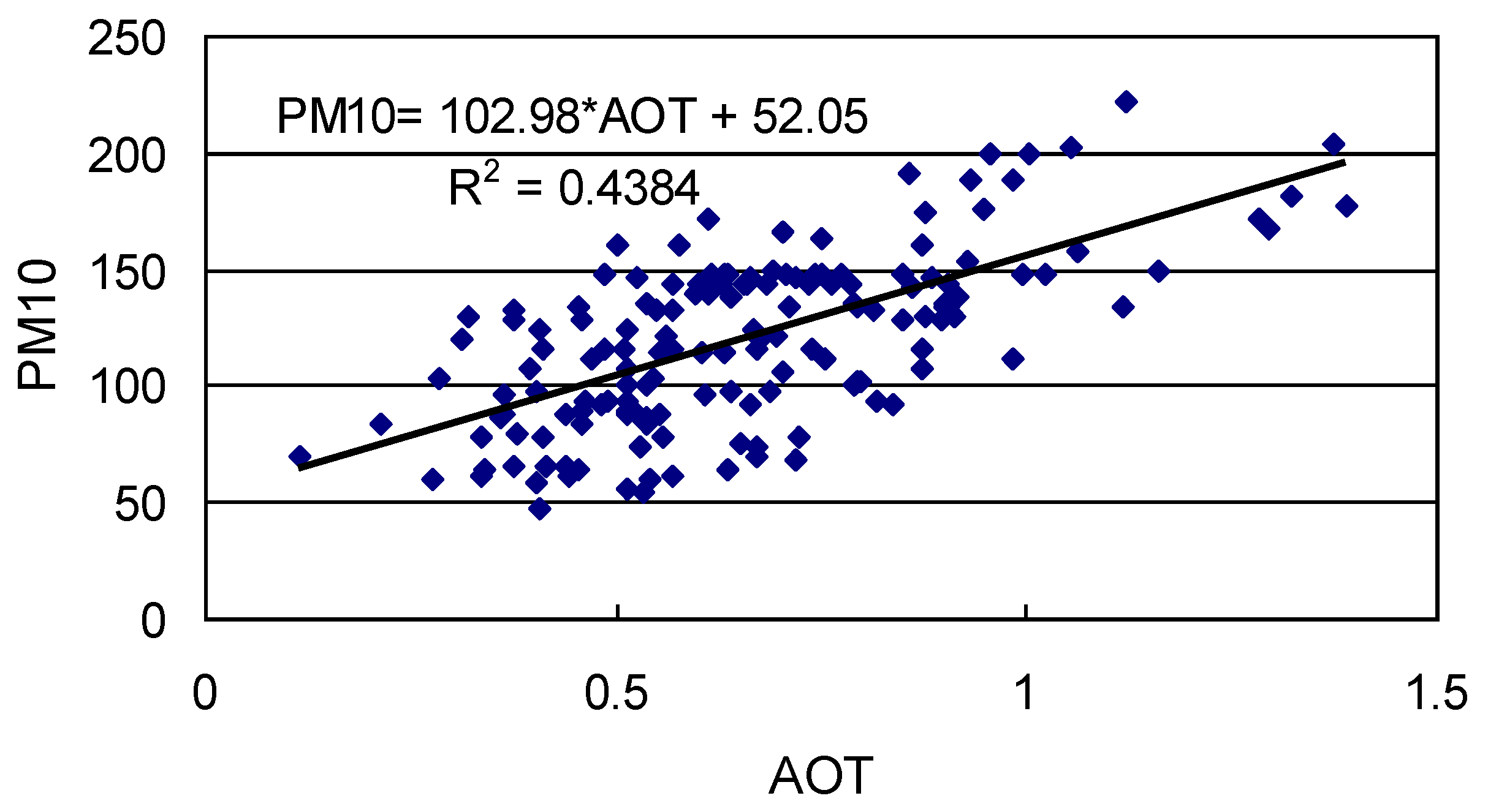
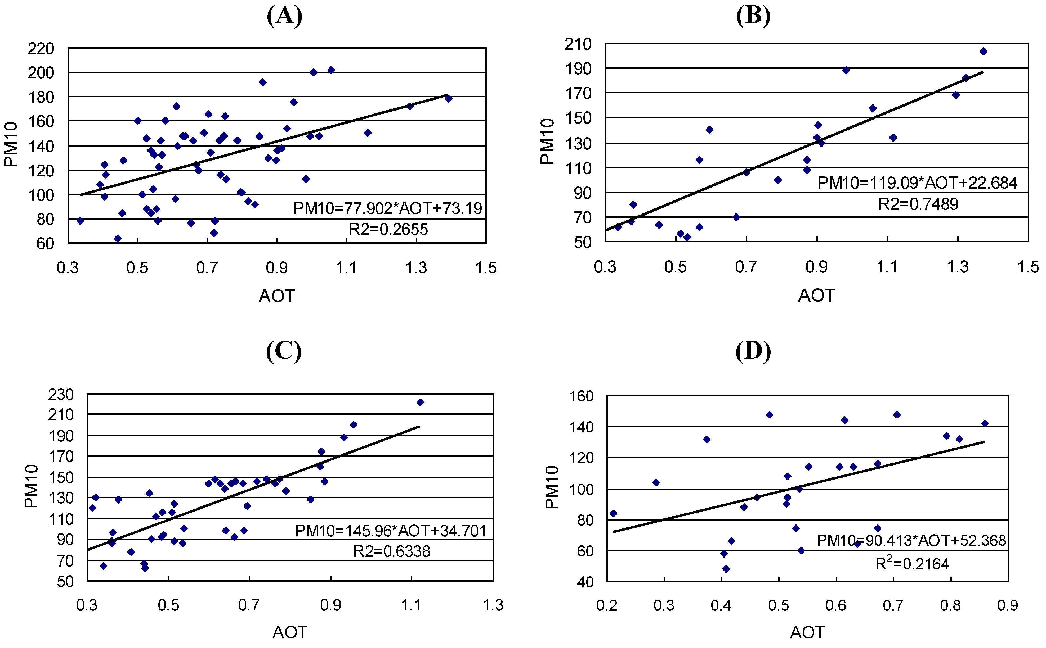
3.1. Relationship between PM₁₀ and AOT and Its Seasonal Variability

The scatterplot of AOT versus PM₁₀ for all the 157 observations (Figure 1) shows that the two have a linear relationship between them. In general, a higher AOT corresponds to a larger PM₁₀. Thus, PM₁₀ was regressed against AOT linearly, with the following model established:

PM₁₀ = 102.98 * AOT + 52.05

(1)

This regressed model has a slightly better prediction accuracy at a larger AOT as the data are scattered more widely at a lower AOT. Its determinant coefficient of R² = 0.438 suggests that it is reasonable to use the satellite-derived AOT products as a proxy of PM₁₀ for the study area.

Figure 1. Scatterplot of AOT versus PM₁₀ based on all 157 observations.

Figure 1. Scatterplot of AOT versus PM₁₀ based on all 157 observations.

In order to explore the seasonality of the regression model, the same analysis was carried out with the seasonally grouped PM₁₀ data. After partitioning, 62 of the 157 observations fall into the spring season, the largest number of observations among the four seasons. On the other hand, only 24 observations are available for the summer season. According to the scatterplots (Figure 2), the relationship between PM₁₀ and AOT in all four seasons can be approximated as linear, even though the closeness of this relationship varies widely from season to season. Therefore, PM₁₀ was linearly regressed against AOT by season. As expected, the accuracy of the regression models varies with seasonality. The regression model is the most accurate (R² = 0.749, n = 24) in summer (Figure 2(B)), and slightly less so (R² = 0.634, n = 45) in autumn (Figure 2(C)), but much lower in spring (R² = 0.266, n = 62) and winter (R² = 0.216, n = 26) (Figure 2(A,D)). Therefore, air pollution can be rather reliably estimated from AOT during June-November (e.g., R² > 0.6), but nearly impossible during December–May (e.g., R² < 0.3). In comparison with the model for the entire dataset (Equation 1), both summer and autumn have an improved accuracy while the accuracy for the spring and winter seasons is lower. In other words, the air pollution conditions recorded in satellite imagery are able to depict the pollution level better during June–November than during the rest of the year [16].

The likely reason to account for the varying degree of prediction accuracy is the meteorological conditions in different seasons that control the circulation of pollutants in the atmosphere. Statistical analysis shows that PM₁₀ has a high correlation coefficient (r > 0.80) with AOT during June–November (Table 1). The correlation coefficient drops to around 0.5 in other two seasons. A close scrutiny of the statistical values of the four meteorological parameters, however, reveals no obvious meteorological patterns that can account for the observed seasonal variation in the correlation. For instance, air pressure is the highest in winter (1,027.15 hPa) and the second highest in autumn (1,020.24 hPa), but is the lowest in summer (1,004.81 hPa). By comparison, temperature is the highest in summer (29.49 °C), but is of a similar level in the mid-10 °C in spring and autumn. Relative humidity (RH) is the highest in autumn (67.49%), but very close in winter and spring at around 53%. The same indefinite relationship exists for wind velocity (WV). Autumn has the calmest weather (1.43 m s⁻¹) while summer is the windiest (2.55 m s⁻¹). The absence of any regularity in the meteorological conditions indicates that rarely a single meteorological variable is solely responsible for the predictability of PM₁₀. Instead, it is the joint effects of several variables that make AOT resemble PM₁₀ closely.

Figure 2. Correlation between PM₁₀ and MODIS-derived AOT data by season. (A) spring; (B) summer; (C) autumn, and (D) winter.

Figure 2. Correlation between PM₁₀ and MODIS-derived AOT data by season. (A) spring; (B) summer; (C) autumn, and (D) winter.

Table 1. Correlation between PM₁₀ and AOT by season and its relationship with meteorological conditions.

Season (coefficient)	Statistical parameter	P (hPa)	T (0C)	RH (%)	WV (m s-1)
Spring (0.52)	AVE	1,015.47	16.27	53.24	2.23
	SD	7.41	6.18	9.78	0.77
Summer (0.87)	AVE	1,004.81	29.49	59.17	2.55
	SD	3.74	2.36	9.09	1.04
Autumn (0.80)	AVE	1,020.24	16.76	67.49	1.43
	SD	4.58	5.23	6.84	0.76
Winter (0.47)	AVE	1,027.15	3.03	52.31	2.07
	SD	5.46	4.01	14.53	1.07

Table 1. Correlation between PM₁₀ and AOT by season and its relationship with meteorological conditions.

Season (coefficient)	Statistical parameter	P (hPa)	T (0C)	RH (%)	WV (m s-1)
Spring (0.52)	AVE	1,015.47	16.27	53.24	2.23
	SD	7.41	6.18	9.78	0.77
Summer (0.87)	AVE	1,004.81	29.49	59.17	2.55
	SD	3.74	2.36	9.09	1.04
Autumn (0.80)	AVE	1,020.24	16.76	67.49	1.43
	SD	4.58	5.23	6.84	0.76
Winter (0.47)	AVE	1,027.15	3.03	52.31	2.07
	SD	5.46	4.01	14.53	1.07

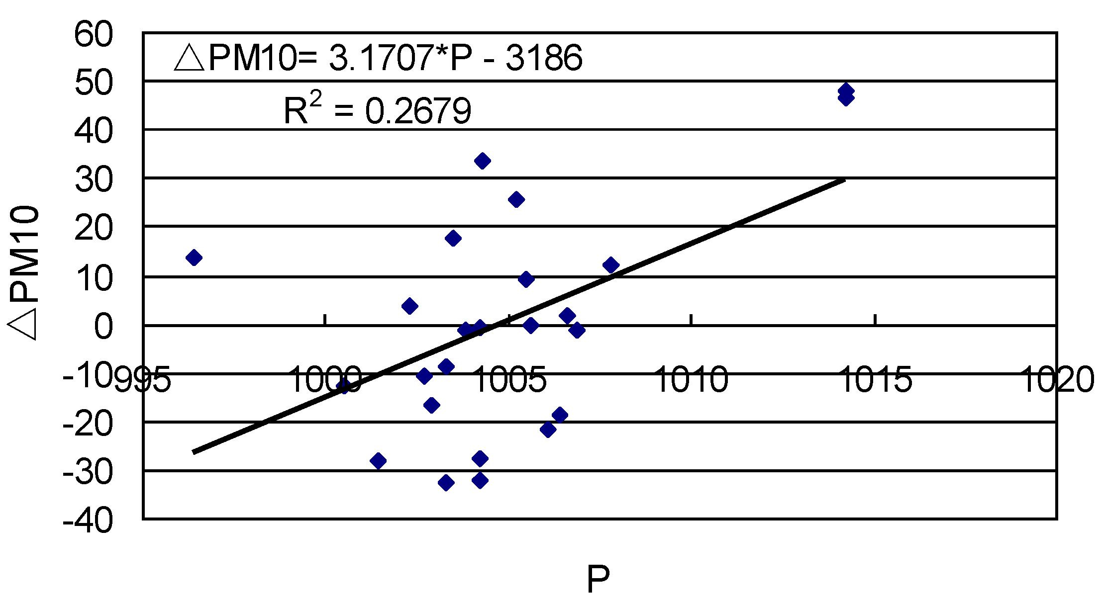
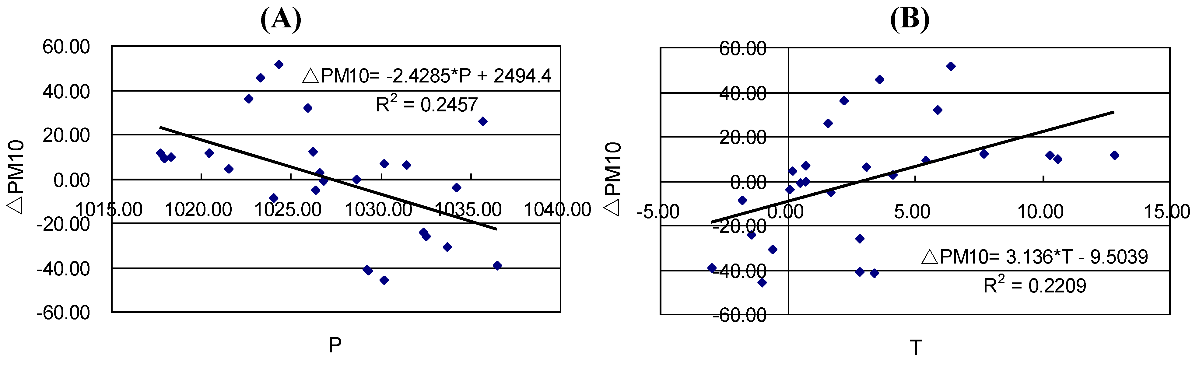
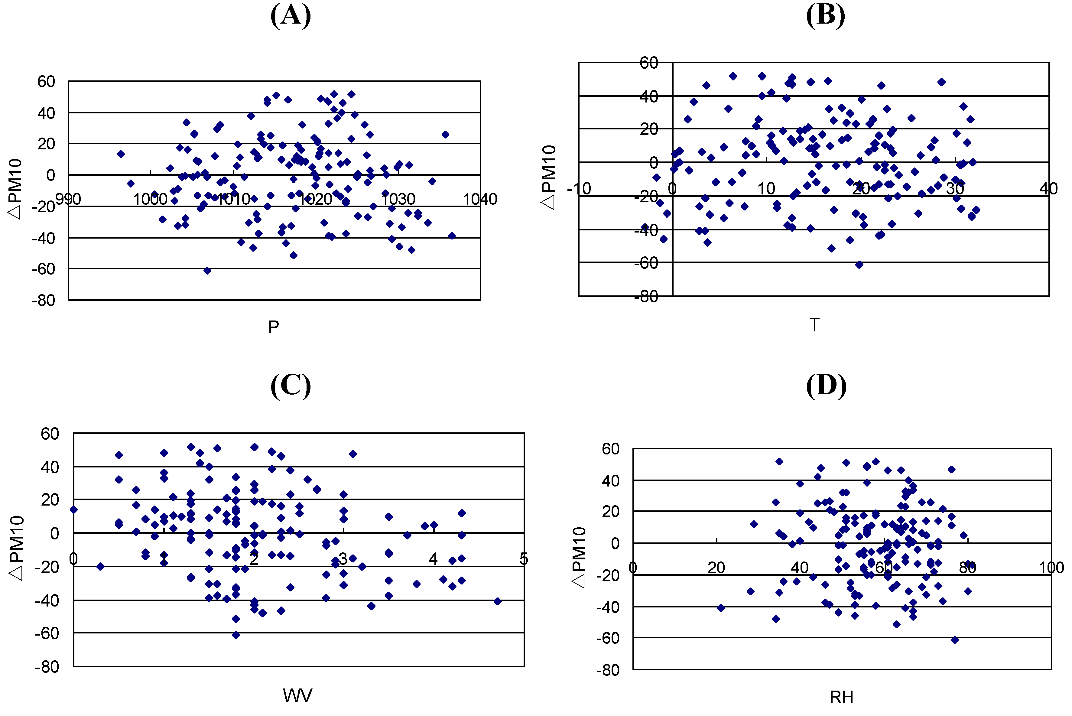
3.2. Meteorological Influence on Residuals of PM₁₀ Estimates

In order to explore the influence of meteorological conditions on the accuracy of predicting PM₁₀, the residuals of PM₁₀ or ΔPM₁₀ are calculated by subtracting the observed PM₁₀ from the PM₁₀ predicted from AOT according to Equation 1. The scatterplots of ΔPM₁₀ versus individual meteorological parameters (Figure 3) demonstrate that no correlation exists between any of them except a weak correlation with WV. This absence shows that under all meteorological conditions, the accuracy of predicting PM₁₀ from AOT cannot be accounted for by any meteorological parameters because the influence of the same parameter is not uniform in different seasons. Moreover, in a given season the cumulative influence of a number of variables is more critical to the predictability of PM₁₀ than individual parameters alone. The interactions among different parameters cause varied concentration levels of air pollutants.

Figure 3. Scatterplots of residuals of PM₁₀ estimates predicted from AOT versus individual meteorological parameters. (A) air pressure; (B) air temperature; (C) wind velocity; and (D) relative humidity.

Figure 3. Scatterplots of residuals of PM₁₀ estimates predicted from AOT versus individual meteorological parameters. (A) air pressure; (B) air temperature; (C) wind velocity; and (D) relative humidity.

In order to explore the seasonal influence of individual meteorological parameters on the predictability of PM₁₀ from AOT, ΔPM₁₀ was calculated again using the regression models in Figure 2 separately by season. The derived residuals were stepwise regressed against the four meteorological parameters individually. It was found that pressure is the most important to the prediction accuracy in summer (Figure 4). It is able to explain 26.79% of the variations in the residuals. By comparison, temperature exerts less influence on the predictability of PM₁₀ probably because they are dependent upon the former variable. This regression model has the following form:

ΔPM₁₀ = −3186 + 3.1707 * P (R² = 0.2679, n = 24)

(2)

The prediction accuracy improves to R² = 0.409 if all the four parameters are used in the regression model (Equation 3). This means that about half of the variations in predicting PM₁₀ from AOT can be accounted for by meteorological influence in this season.

ΔPM₁₀ = −1,591.636 + 1.680 * P − 0.2725 * T+0.030 * RH − 7.201 * WV (R² = 0.409)

(3)

Figure 4. Scatterplot of residuals of PM₁₀ estimates predicted from AOT against pressure (P) in the summer season.

Figure 4. Scatterplot of residuals of PM₁₀ estimates predicted from AOT against pressure (P) in the summer season.

In the winter season, the most important meteorological parameters influencing the accuracy of predicting PM₁₀ from AOT are air pressure and air temperature. As shown in Figure 5(A), a higher pressure corresponds to a lower residual, either positive or negative. A medium pressure is hence more conducive to higher prediction accuracy. Air pressure alone is able to explain a quarter of the variations in the residuals. There is a positive relationship between the residuals and air temperature (Figure 5(B)). Namely, a very high air temperature results in a larger prediction residual. At R² = 0.2209, air temperature exerts a less significant impact on the predictability of PM₁₀ than air pressure (R² = 0.2457). The regression model for ΔPM₁₀ from these two parameters takes the following form:

ΔPM₁₀ = 1,624.626 − 1.604 * P + 1.643 * T (R² = 0.278)

(4)

Figure 5. Scatterplots of residuals in predicting PM₁₀ from AOT in the winter season against the two most important variables. (A) air pressure; (B) air temperature.

Figure 5. Scatterplots of residuals in predicting PM₁₀ from AOT in the winter season against the two most important variables. (A) air pressure; (B) air temperature.

With an R² value of 0.278, this model is marginally more accurate than the two individual models. This means that the joint influence of both parameters is lower than the combined influence of the two parameters. The modeling accuracy of ΔPM₁₀ rises further to R² = 0510 if all the four parameters are used as the exploratory variables in the regression model (Equation 5). This value is considerably higher than 0.278 achieved with the two parameters. Therefore, the four parameters are almost equally important in affecting the residuals of PM₁₀ estimates. The accuracy level of 0.510 is rather comparable to 0.409 for the summer season. Thus, the influence of meteorological parameters on the accuracy of predicting air pollutants from AOT does not vary significantly across the summer and winter seasons. However, the meteorological parameters that are important to the prediction may change. In both seasons RH does not play a significant role in affecting the accuracy of modeling ΔPM₁₀.

ΔPM₁₀ = 1,382.411 − 1.306 * P + 2.761 * T − 0.353 * RH − 15.176 * WV (R² = 0.510)

(5)

Similar regression analysis was carried out for the spring and fall seasons, but the regression models have a rather low R² value of <0.2. This suggests that the correlation between PM₁₀ and AOT as shown in Table 1 bears no relationship with the influence of meteorological factors on the accuracy of predicting PM₁₀ from AOT. A close correlation in summer and autumn does not necessarily mean a predictable influence of meteorological variables on the residuals of estimating PM₁₀ from AOT. This is explained by the fact that AOT has a kind of range of tolerance of meteorological conditions. In spring and autumn when temperature lies in its middle range, any variation within this range will not exert an apparent influence on the residuals. Temperature is extremely low in winter, but extremely high in summer. In both extreme conditions, any change in temperature over the tolerance level will have an immediate impact on the residuals. Once the threshold is crossed, a slight meteorological variation would induce a noticeable change to the atmospheric stability and composition.

4. Discussion

In the constructed prediction model for PM₁₀ in the four seasons, the highest R² value was achieved at 0.749 for the summer season. The model for predicting the residuals of PM₁₀ estimates has a lower R² value of 0.510 from the four meteorological parameters for the same season. A higher accuracy cannot be achieved for two reasons: the number of meteorological parameters used, and differential scales of measurement.

4.1. Selection of Meteorological Parameters

The selection of temperature and relative humidity for the analysis is justified by the fact that heat and moisture controls the stability of the boundary layer while air pressure and wind velocity affects the dispersion of air pollutants and thus aerosol vertical profile. In addition to these four meteorological factors, two more meteorological parameters of rainfall and wind direction may also exert some influence. These two parameters, especially rainfall, play a deterministic role in regulating the quantity of particulate pollutants. For instance, the amount of pollutants is drastically reduced following a rain event. However, the influence of rainfall is haphazard and almost impossible to be taken into consideration in the analysis. Similarly, wind direction affects the dispersion of pollutants. The influence of wind direction is further complicated by surface relief (e.g., topography and buildings). Thus, it is impossible to examine this influence quantitatively, even though its role is minor in comparison with rainfall.

4.2. Differential Scales of Measurement of Air Pollutants

The prediction accuracy cannot reach 100% because PM₁₀ and AOT are not synonymous to each other. Governed by the mass of particulates, PM₁₀ reflects the concentrations of solid pollutants stemming from vehicles, dust storms, and chimneys at or near the Earth’s surface. It does not encompass such gaseous pollutants as CO, SO₂ and NO₂. As impurities suspended in the atmosphere, particulates has a concentration level prone to changes induced by air turbulences, atmospheric instability, and vertical mixing of different layers. Furthermore, PM₁₀ is measured at fixed points at or near the surface. Thus, it is indicative of the pollutant concentration at a particular altitude. By comparison, AOT reflects the cumulative attenuation of the solar radiation in a column over the sampling area (e.g., pixel size measured in square kilometers). It is determined by the total amount of aerosols over the air column and their diameter. As such, it exhibits a distinct spatiotemporal pattern of variation. For instance, in the Sichuan Basin the mean AOT is maximized in spring due to the influence of dust storms [17]. This discrepancy in meaning and measurement scale raises two important implications for the predictability of PM₁₀. First, the prediction accuracy as reported in this study is replicable only if the air pollutants are dominated by solid particulates. Second, the point-based observation at a monitoring station cannot be fully representative of the concentration level sensed over an area equivalent of the pixel size enumerated in 100 km².

Apart from spatial discrepancy, the varying temporal scales of observation also degrade the accuracy of predicting air pollution from AOT. PM₁₀ is an average of observations over the 24 hour cycle. By comparison, the pollutant concentration level remotely detected by the MODIS sensor from space is just a snapshot. Unless the meteorological conditions stay unchanged during a day, it is impossible for the satellite-derived data to accurately depict the reality. Only under those meteorological conditions that change little during the 24-hour period can air pollution be reliably predicted from AOT. The abundant rainfall events in spring prevent a reliable regression model to be established for ΔPM₁₀.

5. Conclusions

The AOT information acquired from the MODIS data is able to reasonably reflect the amount of suspended particulates in the atmosphere. Air pollutants can be predicted from AOT at an accuracy level of R² = 0.438 during the study period. Seasonally, the prediction formulae take the form of PM₁₀ = 119.09 * AOT + 22.684 (R² = 0.749, n = 24) for summer and PM₁₀ = 145.96 * AOT + 34.701 (R² = 0.634, n = 45) for autumn. Therefore, the relationship is very accurate in summer and autumn, but not so accurate in the spring and winter seasons. Further analyses of individual meteorological parameters in different seasons did not yield any definite meteorological pattern that can account for the varying levels of prediction accuracy of PM₁₀. Furthermore, the residuals of PM₁₀ estimates from AOT are loosely correlated with individual meteorological parameters. Seasonally, the residuals in predicting PM₁₀ from AOT are affected by meteorological parameters. In the summer season air pressure is the most important. It alone can account for more than a quarter of the variations in ΔPM₁₀. This accuracy level rises to R² = 0.409 if all the four parameters are used in the prediction in the form of ΔPM₁₀ = −1,591.636 + 1.680 * P−0.2725 * T + 0.030 * RH − 7.201 * WV. In winter, air pressure and air temperature become the parameters important to the accuracy of prediction in the form of ΔPM₁₀ = 1,624.626 − 1.604 * P + 1.643 * T (R² = 0.278). If all four parameters are used in the prediction, the accuracy nearly doubles to R² = 0.510. Therefore, in both seasons the meteorological influence on ΔPM₁₀ remains little changed while the most influential meteorological parameter has not changed. No such relationship can be established in the spring and autumn seasons. Therefore, different meteorological variables are important to the prediction accuracy in different seasons. Higher accuracy cannot be achieved due to the temporal discrepancy between ground observations and the snapshot nature of the satellite imagery, as well as differential spatial scales of measurement. It is concluded that meteorological parameters have a varied influence on the predictability of air pollution from the MODIS data-derived AOT data in an urban area where air pollutants are dominated by suspended particulates.

References

1. Wang, H.; Zha, Y. MODIS-derived aerosol optical thickness as an indicator of urban air quality. Urban Environ. Urban Eco. 2006, 193, 21–24. [Google Scholar]
2. Mao, J.T.; Li, C.C.; Zhang, J.H.; Liu, X.Y.; Lau, A.K.H. The comparison of remote sensing aerosol optical depth from MODIS data and ground sun2photometer observations. J. Appl. Meteorol. Sci. 2002, 13, 127–135. [Google Scholar]
3. Engel-Cox, J.A.; Hoff, R.M.; Haymet, A.D.J. Recommendations on the use of satellite remote-sensing data for urban air quality. J. Air Waste Manag.t Assoc. 2004a, 54, 1360–1371. [Google Scholar] [CrossRef]
4. Chu, D.A.; Kaufman, Y.J.; Zibordi, G.; Chern, J.D.; Mao, J.; Li, C.C.; Holben, B.N. Global monitoring of air pollution over land from the Earth Observing System-Terra Moderate Resolution Imaging Spectroradiometer (MODIS). J. Geophys. Res. 2003, 108. [Google Scholar] [CrossRef]
5. Engel-Cox, J.A.; Holloman, C.H.; Coutant, B.W.; Hoff, R.M. Qualitative and quantitative evaluation of MODIS satellite sensor data for regional and urban scale air quality. Atmos. Environ. 2004, 38, 2495–2509. [Google Scholar] [CrossRef]
6. Hutchison, K.D. Applications of MODIS satellite data and products for monitoring air quality in the state of Texas. Atmos. Environ. 2003, 37, 2403–2412. [Google Scholar] [CrossRef]
7. Li, C.C.; Lau, A.K.H.; Mao, J.; Chen, A. An aerosol pollution episode in Hong Kong with remote sensing products of MODIS and LIDAR. J. Appl. Meteorol. Sci. 2004, 15, 641–651. [Google Scholar]
8. Liu, G.Q.; Li, C.C.; Zhu, A.H.; Mao, J.T. Optical depth research of atmospheric aerosol in the Yangtze River Delta region. Environ. Protection 2003, 8, 50–54. [Google Scholar]
9. Wang, J.; Christopher, S.A. Intercomparison between satellite-derived aerosol optical thickness and PM2.5 mass: Implications for air quality studies. Geophys. Res. Lett. 2003, 30. [Google Scholar] [CrossRef]
10. Li, C.C.; Mao, J.T.; Lau, A.K.H.; Liu, X.Y.; Liu, G.Q.; Zhu, A.H. Research on the air pollution in Beijing and its surroundings with MODIS AOD products. Chin. J. Atmos. Sci. 2003a, 27, 869–880. [Google Scholar]
11. Li, C.C.; Mao, J.T.; Lau, A.K.H.; Yuan, Z.B.; Wang, M.H.; Liu, X.Y. Application of MODIS satellite products to the air pollution research in Beijing. Sci. China Series D-Earth Sci. 2005, 48 (Suppl), 209–219. [Google Scholar]
12. Beran, D.W.; Hall, F.F. Remote-sensing for air-pollution meteorology. Bull. Amer. Meteorol. Soc. 1974, 55, 1097–1105. [Google Scholar] [CrossRef]
13. King, M.D.; Kaufman, Y.J.; Menzel, W.P.; Tanré, D. Remote sensing of cloud, aerosol, and water vapor properties from the Moderate Resolution Imaging Spectrometer (MODIS). IEEE Trans. Geosci. Remote Sens. 1992, 30, 2–27. [Google Scholar] [CrossRef]
14. Kaufman, Y.J.; Tanr, D.; Remer, L.A.; Vermote, E.F.; Chu, A.; Holben, B.N. Operational remote sensing of tropospheric aerosol over the land from EOS-MODIS. J. Geophys. Res. 1997, 102, (D14). 17051–17068. [Google Scholar] [CrossRef]
15. Kaufman, Y.J.; Wald, A.E.; Remer, L.A.; Gao, B.-C.; Li, R.-R.; Flynn, L. The MODIS 2.1 μm channel—Correlation with visible reflectance for use in remote sensing of aerosol. IEEE Trans. Geosci. Remote Sens. 1997, 35, 1286–1298. [Google Scholar] [CrossRef]
16. Zha, Y.; Gao, J.; Jiang, J.; Lu, H.; Huang, J. Monitoring of urban air pollution from MODIS aerosol data: Effect of meteorological parameters. Tellus 2010, 62B, 109–116. [Google Scholar] [CrossRef]
17. Li, C.C.; Mao, J.T.; Lau, A.K.H. Characteristics of aerosol optical depth distributions over Sichuan basin derived from MODIS data. J. Appl. Meteorol. Sci. 2003b, 14, 1–7. [Google Scholar]